hep-ph/0101152

‘Strategy of Regions’:
Expansions of Feynman Diagrams
both in Euclidean and
Pseudo-Euclidean Regimes

V.A. Smirnov

Nuclear Physics Institute of Moscow State University
Moscow 119899, Russia

The strategy of regions [1] turns out to be a universal method for expanding Feynman integrals in various limits of momenta and masses. This strategy is reviewed and illustrated through numerous examples. In the case of typically Euclidean limits it is equivalent to well-known prescriptions within the strategy of subgraphs. For regimes typical for Minkowski space, where the strategy of subgraphs has not yet been developed, the strategy of regions is characterized in the case of threshold limit, Sudakov limit and Regge limit.

Presented at the

5th International Symposium on Radiative Corrections
(RADCOR–2000)
Carmel CA, USA, 11–15 September, 2000

1 Introduction

The problem of asymptotic expansions of Feynman integrals in momenta masses is very important and has been analyzed in a large number of papers. For limits typical for Euclidean space, an adequate solution has been found [2] (see a brief review in [3]) and mathematically proven. It is expressed by a simple formula with summation in a certain family of subgraphs of a given graph so that let us refer to it as ‘the strategy of subgraphs’. For limits typical for Minkowski space, the strategy of subgraphs has not yet been rigorously developed.

Quite recently a new method for expanding Feynman integrals in limits of momenta and masses has been suggested [1]. It is based on the analysis of various regions in the space of loop momenta of a given diagram and denoted as ‘the strategy of regions’. The purpose of this talk is to review and illustrate this strategy through numerous examples. First, the problem of asymptotic expansion in limits of momenta and masses is characterized. Then the two basic strategies are formulated and compared for limits typical for Euclidean space. For regimes typical for Minkowski space, the strategy of regions is checked through typical examples, up to two-loop level, in the case of threshold limit, Sudakov limit and Regge limit. Finally, the present status of the strategy of regions is characterized.

2 Limits of momenta and masses

Let $\Gamma$ be a graph and $F_{\Gamma}(m_{1},m_{2},\ldots,q_{1},q_{2},\ldots)$ the corresponding Feynman integral constructed according to Feynman rules and depending on masses $m_{i}$ and external momenta $q_{j}$. It can be represented as a linear combination of tensors composed of the external momenta with coefficients which are scalar Feynman integrals that depend on the masses and kinematical invariants $s_{ij}=q_{i}\!\cdot\!q_{j}$.

The problem of asymptotic expansion of Feynman integrals in some limit of momenta and masses is of the physical origin and arises quite naturally. If one deals with phenomena that take place at a given energy scale it is natural to consider large (small) all the masses and kinematical invariants that are above (below) this scale. Therefore a limit (regime) is nothing but a decomposition of the given family of these parameters into small and large ones.

For limits typical for Euclidean space, an external momentum is called large if at least one of its components is large and small if all its four components are large. Thus such a limit is characterized by a decomposition $\{m_{i}\},\{q_{i}\}\to\{m_{i}\},\{q_{i}\};\{M_{i}\},\{Q_{i}\}$, with $m_{i},|q_{j}|\ll M_{i^{\prime}},|Q_{j^{\prime}}|$, where $|q_{j}|$ is understood in the Euclidean sense.

For limits typical for pseudo-Euclidean space, it is impossible to characterize the external momenta in this way and one turns to a decomposition written through kinematical invariants: $\{m_{i}\},\{s_{jj^{\prime}}\}\to\{m_{i}\},\{s_{jj^{\prime}}\};\{M_{i}\},\{S_{jj^{\prime}}\}$, with $m_{i},|s_{jj^{\prime}}|\ll M_{i^{\prime}},|S_{jj^{\prime}}|$. However, instead of the kinematical invariants themselves, some linear combinations can be used (for example, in the case of the threshold limit).

Feynman integrals are generally quite complicated functions depending on a large number of arguments. When a given Feynman integral is considered in a given limit it looks natural to expand it in ratios of small and large parameters and then replace the initial complicated object by a sufficiently large number of first terms of the corresponding asymptotic expansion. Experience shows that Feynman integrals are always expanded in powers and logarithms of the expansion parameter which is a ratio of the large and the small scales of the problem. In particular, when a given Feynman integral depends only on a small mass squared and a large external momentum squared, $m^{2}\ll-q^{2}$, we have

$$F_{\Gamma}(q^{2},m^{2})\sim(-q^{2})^{\omega}\sum_{n=n_{0}}^{\infty}\sum_{j=0}^{2h}C_{nj}\,\left(\frac{m^{2}}{-q^{2}}\right)^{n}\ln^{j}\left(\frac{m^{2}}{-q^{2}}\right)\;,$$ (1)

where $h$ is the number of loops of $\Gamma$ and $\omega$ ultraviolet (UV) degree of divergence. The maximal power of the logarithm equals the number of loops for typically Euclidean limits and is twice the number of loops for limits typical for Minkowski space.

To expand Feynman diagrams one can either

1. Take a given diagram in a given limit and expand it by some special technique, or,

2. Formulate prescriptions for a given limit and then apply them to any diagram (e.g. with 100 loops).

Of course, the second (global) solution is preferable because

• no analytical work is needed when applying it to a given diagram: just follow formulated prescriptions and write down a result in terms of Feynman integrals (with integrands expanded in Taylor series in some parameters);

• a natural requirement can be satisfied: individual terms of the expansion are homogeneous (modulo logs) in the expansion parameter.

Two kinds of such global prescriptions are known:

• Strategy of Subgraphs and

• Strategy of Regions

We shall now formulate both strategies in the case of limits typical for Euclidean space.

3 Strategy of subgraphs and strategy of regions for limits typical for Euclidean space

For limits typical for Euclidean space, the solution of the problem of asymptotic expansion is described [2] by the following simple formula, with summation in subgraphs, supplied with some explanations:

$$F_{\Gamma}\sim\sum_{\gamma}F_{\Gamma/\gamma}\circ{\cal T}_{\gamma}F_{\gamma}\;,$$ (2)

where the sum runs in a certain class of subgraphs $\gamma$ of $\Gamma$. For example, in the off-shell (Euclidean) limit $m^{2}\ll-q^{2}$ (when $q$ is considered large in Euclidean sense), one can distribute the flow of $q$ through all the lines of $\gamma$. (This is a ‘physical’ definition.) Moreover $F_{\gamma}$ and $F_{\Gamma/\gamma}$ are the Feynman integrals respectively for $\gamma$ and $\Gamma/\gamma$ (the reduced graph $\Gamma/\gamma$ is obtained from $\Gamma$ by collapsing $\gamma$ to a point). The operator ${\cal T}_{\gamma}$ expands the integrand of $F_{\gamma}$ in Taylor series in its small masses and small external momenta which are either the small external momenta of $\Gamma$, or loop momenta of the whole graph that are external for $\gamma$ (they are by definition small). The symbol $\circ$ denotes insertion of the second factor (polynomial) into $F_{\Gamma/\gamma}$ (like an insertion of a counterterm within dimensional renormalization).

All quantities are supposed to be dimensionally regularized [4] by $d=4-2\varepsilon$. Even if the initial Feynman integral is UV and IR finite, the regularization is necessary because individual terms in the right-hand side become divergent starting from some minimal order of expansion. The necessity to run into divergences is a negligible price to have the simplest prescription for expanding Feynman integrals. Moreover the cancellation of divergences in the right-hand side of expansions of finite Feynman integrals is a very crucial practical check of the expansion procedure.

Operator analogs of limits typical for Euclidean space (the off-shell large momentum limit and the large mass limit) are operator product expansion and large mass expansion described by an effective Lagrangian — see a review with applications in [5].

Consider, for example, the scalar diagram shown in Fig. 1 in the off-shell limit $m^{2}\ll-q^{2}$ which can treated as a Euclidean limit with the external momentum $q$ large in the Euclidean sense.

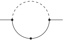
Figure 1: One-loop propagator diagram

The propagator of the dashed line is massless and the dot on the solid line denotes the second power of the massive propagator. The corresponding Feynman integral is

$$F_{\Gamma}(q^{2},m^{2};\varepsilon)=\int\frac{\mbox{d}^{d}k}{(k^{2}-m^{2})^{2}(q-k)^{2}}\;.$$ (3)

The causal $i0$ in the propagators $k^{2}-m^{2}+i0$, etc. are omitted for brevity.

According to (2) two subgraphs give non-zero contributions. The graph $\Gamma$ itself generates Taylor expansion of the integrand in $m$, with resulting massless integrals evaluated (e.g. by Feynman parameters) in gamma functions for general $\varepsilon$:

$$\int\frac{\mbox{d}^{d}k}{(q-k)^{2}}{\cal T}_{m}\frac{1}{(k^{2}-m^{2})^{2}} = \int\frac{\mbox{d}^{d}k}{(k^{2})^{2}(q-k)^{2}}-2m^{2}\int\frac{\mbox{d}^{d}k}{(k^{2})^{3}(q-k)^{2}}+\ldots$$ (4)

$$= \frac{i\pi^{d/2}}{(-q^{2})^{1+\varepsilon}}\frac{\Gamma(1-\varepsilon)^{2}\Gamma(\varepsilon)}{\Gamma(1-2\varepsilon)}\left[1+2\varepsilon\frac{m^{2}}{q^{2}}+\ldots\right]\;.$$

The second contribution originates from the subgraph $\gamma_{1}$ which is the upper line. It is given by Taylor expansion of its propagator in the loop momentum $k$ which is external for this subgraph, with resulting massive vacuum integrals also evaluated in gamma functions for general $\varepsilon$:

$$\int\frac{\mbox{d}^{d}k}{(k^{2}-m^{2})^{2}}{\cal T}_{k}\frac{1}{(q-k)^{2}} = \frac{1}{q^{2}}\int\frac{\mbox{d}^{d}k}{(k^{2}-m^{2})^{2}}+\frac{1}{(q^{2})^{2}}\int\frac{(2q\!\cdot\!k-k^{2})\mbox{d}^{d}k}{(k^{2}-m^{2})^{2}}+\ldots$$ (5)

$$= \frac{i\pi^{d/2}}{q^{2}(m^{2})^{\varepsilon}}\Gamma(\varepsilon)\left[1+\frac{\varepsilon}{1+\varepsilon}\frac{m^{2}}{q^{2}}+\ldots\right]\;.$$

The contribution of another subgraph consisting of two lower lines generates a zero contribution because this is a massless vacuum diagram:

$$\int\frac{\mbox{d}^{d}k}{k^{2}}{\cal T}_{k,m}\frac{1}{((q-k)^{2}-m^{2})^{2}}=\frac{1}{(q^{2})^{2}}\int\frac{\mbox{d}^{d}k}{k^{2}}+\ldots=0\;.$$

This contribution would be however non-zero in the case of a non-zero mass in the lower lines.

When $\varepsilon\to 0$, infrared (IR) poles in the first non-zero contribution are canceled against ultraviolet (UV) poles in the second one, with the finite result

$$F_{\Gamma}(q^{2},m^{2};0)\sim\frac{i\pi^{2}}{q^{2}}\left[\ln\left(\frac{-q^{2}}{m^{2}}\right)-\frac{m^{2}}{q^{2}}+\ldots\right]\;.$$ (6)

It turns out that at present there are no simple generalizations of the strategy of subgraphs to typical Minkowskian regimes. Before formulating what the strategy of regions is let us remind that a (standard) strategy of regions was used for many years for analyzing leading power and (sub)leading logarithms. It reduces to the following prescriptions:

• Consider various regions of the loop momenta and expand, in every region, the integrand in a Taylor series with respect to the parameters that are considered small in the given region;

• pick up the leading asymptotic behaviour generated by every region.

Let us stress that cut-offs that specify the regions are not removed within this strategy. In fact, it was sufficient to analyze rather limited family of regions because the leading asymptotics are generated only by specific regions.

The (generalized) strategy of regions has been suggested in [1] (and immediately applied to the threshold expansion):

• Consider various regions …

• Integrate the integrand expanded, in every region in its own way, over the whole integration domain in the loop momenta;

• Put to zero any integral without scale.

Let us stress that, for typically Euclidean limits, integrals without scale (tadpoles) are automatically put to zero. For general limits, this is an ad hoc prescription.

An experimental observation tell us that this strategy of regions gives asymptotic expansions for any diagram in any limit. In particular, it has been checked in numerous examples when comparing results of expansion with existing explicit analytical results. We have also an indirect confirmation because, for limit typical for Euclidean space, the strategy of regions leads to the same prescriptions as the strategy of subgraphs. To see this it is in fact sufficient to take any loop momentum to be either

$$large: k\sim q\;,\;\;\;\;\mbox{or}$$

$$small: k\sim m$$

and then observe that one obtains eq. (2).

Still to see how the strategy of regions works let us consider the previous example of Fig. 1. We consider the loop momentum $k$ to be either large or small and obtain

$$k\;\mbox{large:} \rightarrow {\cal T}_{m}\frac{1}{(k^{2}-m^{2})^{2}}\leftrightarrow\Gamma$$

$$k\;\mbox{small:} \rightarrow {\cal T}_{k}\frac{1}{(q-k)^{2}}\leftrightarrow\gamma_{1}$$

Thus the region of the large momenta reproduces the contribution of the subgraph $\Gamma$ and the region of the small momenta reproduces the contribution of the subgraph $\gamma_{1}$ present according to the strategy of subgraphs (2).

From now on we turn to various examples of limits typical for Minkowski space.

4 Strategy of regions for limits typical for Minkowski space

4.1 Threshold expansion [1]

Consider first the threshold limit when an external momentum squared tends to a threshold value. Our primary task is to see what kinds of regions are relevant here. Let us consider the same example of Fig. 1 but in the new limit, $q^{2}\to m^{2}$. In this case, it is reasonable to choose the loop momentum in another way to make explicit the dependence on the expansion parameter:

$$F_{\Gamma}(q^{2},y;\varepsilon)=\int\frac{\mbox{d}^{d}k}{k^{2}((q-k)^{2}-m^{2})^{2}}=\int\frac{\mbox{d}^{d}k}{k^{2}(k^{2}-2q\!\cdot\!k-y)^{2}}\;.$$ (7)

So we have turned to the new variables $(q^{2},m^{2})\rightarrow(q^{2},y)$ with $y=m^{2}-q^{2}\to 0$ the expansion parameter of the problem.

Let us look for relevant regions. The region of large (let us from now on use the term hard instead) momenta, $k\sim q$, always contributes. It gives

$$\int\frac{\mbox{d}^{d}k}{k^{2}}{\cal T}_{y}\frac{1}{(k^{2}-2q\!\cdot\!k-y)^{2}}=\int\frac{\mbox{d}^{d}k}{k^{2}(k^{2}-2q\!\cdot\!k)^{2}}+\ldots=\frac{i\pi^{d/2}}{(q^{2})^{1+\varepsilon}}\frac{\Gamma(1+\varepsilon)}{2\varepsilon}+\ldots,$$ (8)

where each integral is evaluated in gamma functions for general $\varepsilon$.

If we consider the region of small loop momenta, $k\sim\sqrt{y}$ (which from now on we will call soft) we shall obtain an integral without scale which we put to zero according to one of the prescriptions of the strategy of regions:

$$\int\frac{\mbox{d}^{d}k}{k^{2}(-2q\!\cdot\!k)^{2}}+\ldots=0\;.$$

It is the ultrasoft (us) region, $k\sim y/\sqrt{q^{2}}$, which gives here the second non-zero contribution:

$$\int\frac{\mbox{d}^{d}k}{k^{2}}{\cal T}_{k^{2}}\frac{1}{(k^{2}-2q\!\cdot\!k-y)^{2}}=\int\frac{\mbox{d}^{d}k}{k^{2}(-2q\!\cdot\!k-y)^{2}}+\ldots\\ =-i\pi^{d/2}\frac{\Gamma(1-\varepsilon)\Gamma(2\varepsilon)}{(q^{2})^{1-\varepsilon}y^{2\varepsilon}}\;.$$

Only the leading term survives because, in the next terms the factor $k^{2}$ resulting from expansion cancels the massless propagator so that a scaleless integral appears.

If we combine the hard and ultrasoft contributions we shall obtain, in the limit $\varepsilon\to 0$, the known explicit result for the given diagram expanded at threshold:

$$\frac{i\pi^{d/2}}{q^{2}}\left[\ln\frac{y}{q^{2}}-\frac{y}{q^{2}}+\ldots\right]\;.$$

It turns out that for diagrams consisting of massless and massive (with the same mass $m$) lines and having thresholds only with one massive line, i.e. at $q^{2}=m^{2}$, only hard and ultrasoft regions are relevant. To find other characteristic regions we turn to an example with two massive lines — see Fig. 2.

Figure 2: One-loop propagator diagram with two non-zero masses in the threshold

We have

$$F_{\Gamma}(q^{2},y;\varepsilon)=\int\frac{\mbox{d}^{d}k}{(k^{2}-m^{2})((q-k)^{2}-m^{2})}=\int\frac{\mbox{d}^{d}k}{(k^{2}+q\!\cdot\!k-y)(k^{2}-q\!\cdot\!k-y)}\;,$$ (9)

where the loop momentum in again chosen in another way, and we have turned to the new variables: $(q^{2},m^{2})\rightarrow(q^{2},y)$ where $y=m^{2}-q^{2}/4\to 0$ is the small parameter of the problem. Keeping in mind the non-relativistic flavour of the problem we choose the frame $q=\{q_{0},\vec{0}\}$.

Let us look for relevant regions. The hard region, $k\sim q$, gives

$$\int\mbox{d}^{d}k{\cal T}_{y}\frac{1}{(k^{2}+q_{0}k_{0}-y)(k^{2}-q_{0}k_{0}-y)}+\ldots = \int\mbox{d}^{d}k\frac{1}{(k^{2}+q_{0}k_{0})(k^{2}-q_{0}k_{0})}+\ldots$$ (10)

$$= i\pi^{d/2}\left(\frac{4}{q^{2}}\right)^{\varepsilon}\frac{\Gamma(\varepsilon)}{1-2\varepsilon}+\ldots$$

The soft and ultrasoft regions generate zero contributions because of the appearance of scaleless integrals:

$$-\frac{1}{q^{2}}\int\frac{\mbox{d}^{d}k}{k_{0}^{2}}+\ldots=0\;,\;\;\;-\frac{1}{q^{2}}\int\frac{\mbox{d}k_{0}\mbox{d}^{d}\vec{k}}{(q_{0}k_{0}-y+i0)(q_{0}k_{0}+y-i0)}+\ldots=0\;.$$ (11)

It turns out that the missing non-zero contribution here comes from the potential (p) [1] region, $k_{0}\sim y/q_{0}\,,\;\vec{k}\sim\sqrt{y}$. It generates Taylor expansion in $k_{0}^{2}$ and is evaluated by closing the integration contour in $k_{0}$ and taking a residue, e.g. in the upper half-plane, and then evaluating $(d-1)$-dimensional integral in $\vec{k}$ using Feynman parameters. Here again only the leading term survives because the next terms involve scaleless integrals:

$$\int\mbox{d}k_{0}\mbox{d}^{d-1}\vec{k}{\cal T}_{k_{0}^{2}}\frac{1}{(k^{2}+q_{0}k_{0}-y+i0)(k^{2}-q_{0}k_{0}-y+i0)}$$ (12)

$$=\int\frac{\mbox{d}k_{0}\mbox{d}^{d-1}\vec{k}}{(\vec{k}^{2}-q_{0}k_{0}+y-i0)(\vec{k}^{2}+q_{0}k_{0}+y-i0)}+\ldots=i\pi^{d/2}\Gamma(\varepsilon-1/2)\sqrt{\frac{\pi y}{q^{2}}}y^{-\varepsilon}\;.$$

The sum of the hard and potential contributions successfully reproduces the known analytical result for the given diagram.

The next example is given by the triangle diagram with two non-zero masses in the threshold — see Fig. 3.

Figure 3: Triangle diagram with two non-zero masses in the threshold

It is considered at $q=p_{1}+p_{2},\;p=(p_{1}-p_{2})/2,\;p_{1}^{2}=p_{2}^{2}=m^{2}$ and is given by the following Feynman integral:

$$\int\frac{\mbox{d}^{d}k}{(k^{2}+q\!\cdot\!k-y)(k^{2}-q\!\cdot\!k-y)(k-p)^{2}}\;,$$ (13)

where again $y=m^{2}-q^{2}/4\to 0$ and $q=\{q_{0},\vec{0}\}$.

The situation is quite similar to the previous diagram. There are two non-zero contributions generated by the hard and potential regions [1]: the (h) contribution

$$\int\mbox{d}^{d}k\frac{1}{(k^{2}+q_{0}k_{0})(k^{2}-q_{0}k_{0})(k-p)^{2}}=-i\pi^{d/2}\left(\frac{4}{q^{2}}\right)^{1+\varepsilon}\frac{\Gamma(\varepsilon)}{2(1+2\varepsilon)}+\ldots$$ (14)

and the (p) contribution

$$\int\frac{\mbox{d}k_{0}\mbox{d}^{d-1}\vec{k}}{(\vec{k}^{2}-q_{0}k_{0}+y-i0)(\vec{k}^{2}+q_{0}k_{0}+y-i0)(-(\vec{k}-\vec{p})^{2})}=i\pi^{d/2}\frac{y^{-\varepsilon}}{\sqrt{q^{2}y}}\frac{\sqrt{\pi}\Gamma(\varepsilon+1/2)}{2\varepsilon}\;.$$ (15)

One can check that their sum equals the whole analytical result for the given diagram.

It turns out that we have already seen the whole list of regions relevant to the threshold expansion, with the qualification that soft regions did not yet contribute in the examples. We refer for two-loop examples to [1]. For example, the threshold expansion of Fig. 4 at $y=m^{2}-q^{2}/4\to 0$ consists of

Figure 4: Two-loop master self-energy diagram with two non-zero masses in the threshold

contributions generated by the following regions: (h-h), (h-p)=(p-h), (p-p), (p-us) (where two loop momenta are characterized, and the ultrasoft momentum in the last contribution refers to the momentum of the middle line).

Similarly, the threshold expansion of Fig. 5 at $y=m^{2}-q^{2}/4\to 0$

Figure 5: Two-loop vertex diagram with two non-zero masses in the threshold

consists of (h-h), (h-p), (p-h), (p-p), (p-s) (where the loop momentum of the box subgraph is soft) and (p-us) (where the momentum of the middle line is ultrasoft) contributions — see details in [1].

It should be stressed that the knowledge about expansions of individual Feynman diagram gives the possibility to derive expansions at the operator level. The threshold expansion with one zero (small) and one non-zero mass in the threshold leads to HQET (see [7] for review), while the situation with two non-zero masses in the threshold provides the transition from QCD to NRQCD [8] and then further to pNRQCD [8]. Historically, the development of HQET was performed without the knowledge of the corresponding diagrammatical expansion. This can be explained by the combinatorial simplicity of HEQT with the structure similar to that of the large mass expansion, where there are only two scales in the problem.

The case of the threshold expansion with two non-zero masses in the threshold is much more complicated. At the diagrammatical level, this is described by the multiplicity of relevant regions in the problem which correspond to three different scales: $m$ (mass of the quark), the momentum $mv$, where $v$ is relative velocity of the quarks (straightforwardly expressed through the variable $y$ in the above examples), and the energy $mv^{2}$. An adequate description of the transition from NRQCD (which is obtained from QCD by ‘integrating out’ the hard scale, $m$) to pNRQCD has been obtained not so easily (see a discussion from the point of view of 1997 in [1]), and the development of the diagrammatical threshold expansion helped to unambiguously identify all relevant scales in the problem and the form of the corresponding terms in the effective Lagrangian.

The threshold expansion resulted in a number of applications. The first of them was analytical evaluation of the two-loop matching coefficients of the vector current in NRQCD and QCD [10]. Another class of important results was the two-loop description of the $t\overline{t}$ production in $e^{+}e^{-}$ annihilation near threshold — see [11].

4.2 Sudakov limit

There are three different versions of the Sudakov limit $m^{2}\ll Q^{2}\equiv-s=-(p_{1}-p_{2})^{2}$ or $M^{2}\ll-s$ which are exemplified by scalar triangle diagram in Fig. 6, where dashed lines denote massless propagators.

Figure 6: Triangle diagram in the Sudakov limit

Within the ‘standard’ strategy of regions, summing up (sub)leading logarithms (at the leading power) using evolution equations has been analyzed in a large number of papers [12].

Let us expand the triangle diagram in Limit A by the strategy of regions. With the standard choice $p_{1,2}=(Q/2,0,0,\mp Q/2)$, we have

$$\int\frac{\mbox{d}^{d}k}{(k^{2}-2p_{1}\!\cdot\!k)(k^{2}-2p_{2}\!\cdot\!k)(k^{2}-m^{2})}$$

$$=\int\frac{\mbox{d}k_{+}\mbox{d}k_{-}\mbox{d}^{d-2}\underline{k}}{(k_{+}k_{-}-\underline{k}^{2}-Qk_{+})(k_{+}k_{-}-\underline{k}^{2}-Qk_{-})(k_{+}k_{-}-\underline{k}^{2}-m^{2})}\;,$$

where $k_{\pm}=k_{0}\pm k_{3},\;\underline{k}=(k_{1},k_{2})$, with $2p_{1,2}\!\cdot\!k=Qk_{\pm}$.

Let us look for relevant regions. The hard region, $k\sim q$, generates Taylor expansion of the integrand in $m^{2}$

$$\int\frac{\mbox{d}^{d}k}{(k^{2}-2p_{1}\!\cdot\!k)(k^{2}-2p_{2}\!\cdot\!k)k^{2}}+\ldots=-i\pi^{d/2}\frac{1}{(Q^{2})^{1+\varepsilon}}\frac{\Gamma(1+\varepsilon)\Gamma(-\varepsilon)^{2}}{\Gamma(1-2\varepsilon)}+\ldots\;.$$ (16)

The soft ($k\sim m$) and ultrasoft ( $k\sim m^{2}/Q$) regions generate scaleless integrals which are zero:

$$\int\frac{\mbox{d}^{d}k}{(-2p_{1}\!\cdot\!k)(-2p_{2}\!\cdot\!k)k^{2}}+\ldots=0\;,\;\;\;\int\frac{\mbox{d}^{d}k}{(-2p_{1}\!\cdot\!k)(-2p_{2}\!\cdot\!k)(-m^{2})}+\ldots=0\;.$$ (17)

What is yet missing is the contribution of collinear regions:

1-collinear (1c): $$k_{+}\sim m^{2}/Q,\,\,k_{-}\sim Q\,,\,\,\underline{k}\sim m\,,$$

2-collinear (2c): $$k_{+}\sim Q,\,\,k_{-}\sim m^{2}/Q\,,\,\,\underline{k}\sim m\,.$$

The (1c) region generates Taylor expansion of propagator 2 in $k^{2}$:

$$\int\frac{\mbox{d}^{d}k}{(k^{2}-2p_{1}\!\cdot\!k)(-2p_{2}\!\cdot\!k)(k^{2}-m^{2})}+\ldots,$$ (18)

and the (2c) contribution is symmetrical. These contributions are not however individually regularized by dimensional regularization. A natural way to overcome this obstacle is to introduce an auxiliary analytic regularization [14], calculate (1c) and (2c) contributions and switch it off in the sum. Then the (1c) and (2c) regions give, in the leading power,

$$-i\pi^{d/2}\frac{\Gamma(\varepsilon)}{Q^{2}(m^{2})^{\varepsilon}}\left[\ln(Q^{2}/m^{2})+\psi(\varepsilon)-\gamma_{\rm E}-2\psi(1-\varepsilon)\right]+\ldots$$ (19)

After we combine the (h) and (c) contributions we shall see that IR/collinear poles in the (h) contribution and UV/collinear poles in (c) contribution are canceled, and at $\varepsilon\to 0$ we obtain

$$\frac{i\pi^{2}}{Q^{2}}\left[\mbox{Li}_{2}(x)-\frac{1}{2}\ln^{2}x+\ln x\ln(1-x)-\frac{\pi^{2}}{3}\right]\,,$$ (20)

where $\mbox{Li}_{2}(x)$ is dilogarithm and $x=m^{2}/Q^{2}$.

The triangle diagrams of Fig. 5 in Limits B and C are similarly expanded. In Limit B one meets (h), (1c), (2c) and (us) regions, and, in Limit C, one has (h), (1c) and (2c) regions.

Two-loop examples for the Sudakov limit, within the strategy of regions, can be found in [15].

Figure 7: Two-loop vertex diagram in Limit A

For example, the following regions contribute to the expansion of Fig. 7 in Limit A: (h-h), (1c-h)$+$(2c-h), (1c-1c)$+$(2c-2c), and (h-s) where the soft momentum refers to the middle line. For Limit B, one has (h-h), (1c-h)$=$(2c-h), (1c-1c)$=$(2c-2c), (us-h), (us-1c), (us-2c), (us-us).

For the diagram of Fig. 5 (considered above in the threshold limit), with $p_{1,2}=\tilde{p}_{1,2}+(m^{2}/Q^{2})\tilde{p}_{2,1}\,,$ with $\tilde{p}_{1,2}=(Q/2,0,0,\mp Q/2)$, obvious regions (h-h), (1c-h)$=$(2c-h), (1c-1c)$=$(2c-2c) are not sufficient because the poles of the fourth order do not cancel. It turns out that it is necessary to consider also ultracollinear regions:

(1uc): $$k_{+}\sim m^{4}/Q^{3},\,\,k_{-}\sim m^{2}/Q\,,\,\,\underline{k}\sim m^{3}/Q^{2}\,,$$

(2uc): $$k_{+}\sim m^{2}/Q,\,\,k_{-}\sim m^{4}/Q^{3}\,,\,\,\underline{k}\sim m^{3}/Q^{2}\,.$$

After one adds contributions of the (1uc-2c) and (1c-2uc) regions the leading power of expansion satisfies the check of poles [15].

The (generalized) strategy of regions combined with evolution equations derived within the ‘standard’ strategy of regions has been applied to summing up next-to-leading logarithms for Abelian form factor and four-fermion amplitude in the $SU(N)$ gauge theory [16].

4.3 Regge limit

The Regge limit for scattering diagrams is characterized as $|t|\ll|s|$, where $s=(p_{1}+p_{2})^{2}$ and $t=(p_{1}+p_{3})^{2}$ are Mandelstam variables.

Figure 8: Box diagram

Let us expand, using the strategy of regions, the box diagram shown in Fig. 8. The Feynman integral is

$$\int\frac{\mbox{d}^{d}k}{(k^{2}+2p_{1}\!\cdot\!k)(k^{2}-2p_{2}\!\cdot\!k)k^{2}(k+p_{1}+p_{3})^{2}}\;.$$ (21)

Let $s=-Q^{2}$, $t=-T$, and let us choose $p_{1,2}=(\mp Q/2,0,0,Q/2)$, and $p_{1}+p_{3}=(T/Q,0,\sqrt{T+T^{2}/Q^{2}},0)$. It turns out that in the Regge limit one meets contributions of (h) and (c) regions. The collinear regions are now characterized as

$$\mbox{(1(2)c):}\;\;\;k_{\pm}\sim T/Q,\,\,k_{\mp}\sim Q\,,\,\,\underline{k}\sim\sqrt{T}\;.$$

The sum of (1c) and (2c) gives, in the leading power, $1/t$,

$$i\pi^{d/2}\frac{\Gamma(-\varepsilon)^{2}\Gamma(1+\varepsilon)}{\Gamma(-2\varepsilon)s(-t)^{1+\varepsilon}}\left[\ln(t/s)+\psi(-\varepsilon)-2\psi(1+\varepsilon)+\gamma_{\rm E}\right]\;.$$ (22)

The hard contribution starts from the NLO. If we sum up the (h) and (c) contributions we shall see that, at $\varepsilon\to 0$, only the LO (c) contribution survives and gives

$$\frac{i\pi^{d/2}e^{-\gamma_{\rm E}\varepsilon}}{st}\left[\frac{4}{\varepsilon^{2}}-\left(\ln(-s)+\ln(-t)\right)\frac{2}{\varepsilon}+2\ln(-s)\ln(-t)-\frac{4\pi^{2}}{3}\right]\;.$$ (23)

In the case of on-shell massless double box, $p_{i}^{2}=0$,

Figure 9: Double box

given by the integral

$$\int\int\frac{\mbox{d}^{d}k\mbox{d}^{d}l}{(l^{2}+2p_{1}\!\cdot\!l)(l^{2}-2p_{2}\!\cdot\!l)(k^{2}+2p_{1}\!\cdot\!k)(k^{2}-2p_{2}\!\cdot\!k)}$$ (24)

$$\times\frac{1}{k^{2}(k-l)^{2}(l+r)^{2}}\equiv\frac{\left(i\pi^{d/2}e^{-\gamma_{\rm E}\varepsilon}\right)^{2}}{(-s)^{2+2\varepsilon}(-t)}\;K(t/s;\varepsilon)\;,$$

there are (h-h), (1c-1c) and (2c-2c) contributions in the Regge limit. The (h-h) contribution starts from the NLO, $t^{0}$, and the (c-c) contribution from LO, $t^{-1}$. This is a result for the sum of the LO and NLO contributions [17]

$$K(x,\varepsilon) = -\frac{4}{\varepsilon^{4}}+\frac{5\ln x}{\varepsilon^{3}}-\left(2\ln^{2}x-\frac{5}{2}\pi^{2}\right)\frac{1}{\varepsilon^{2}}$$ (25)

$$-\left(\frac{2}{3}\ln^{3}x+\frac{11}{2}\pi^{2}\ln x-\frac{65}{3}\zeta(3)\right)\frac{1}{\varepsilon}+\frac{4}{3}\ln^{4}x+6\pi^{2}\ln^{2}x-\frac{88}{3}\zeta(3)\ln x+\frac{29}{30}\pi^{4}$$

$$+2x\left[\frac{1}{\varepsilon}\left(\ln^{2}x-2\ln x+\pi^{2}+2\right)-\frac{1}{3}\left(4\ln^{3}x+3\ln^{2}x\right.\right.$$

$$\left.\left.+(5\pi^{2}-36)\ln x+2(33+5\pi^{2}-3\zeta(3))\right)\right]+O(x^{2}\ln^{3}x)\;.$$

The on-shell double box has provided a curious example of a situation when the evaluation of large number terms of the expansion is rather complicated while an explicit analytical result [18] is known:

$$K(x,\varepsilon) = -\frac{4}{\varepsilon^{4}}+\frac{5\ln x}{\varepsilon^{3}}-\left(2\ln^{2}x-\frac{5}{2}\pi^{2}\right)\frac{1}{\varepsilon^{2}}$$ (26)

$$-\left(\frac{2}{3}\ln^{3}x+\frac{11}{2}\pi^{2}\ln x-\frac{65}{3}\zeta(3)\right)\frac{1}{\varepsilon}+\frac{4}{3}\ln^{4}x+6\pi^{2}\ln^{2}x-\frac{88}{3}\zeta(3)\ln x+\frac{29}{30}\pi^{4}$$

$$-\left[2{\mbox{Li}}_{3}\left(-x\right)-2\ln x{\mbox{Li}}_{2}\left(-x\right)-\left(\ln^{2}x+\pi^{2}\right)\ln(1+x)\right]\frac{2}{\varepsilon}$$

$$-4\left(S_{2,2}(-x)-\ln xS_{1,2}(-x)\right)+44{\mbox{Li}}_{4}\left(-x\right)-4\left(\ln(1+x)+6\ln x\right){\mbox{Li}}_{3}\left(-x\right)$$

$$+2\left(\ln^{2}x+2\ln x\ln(1+x)+\frac{10}{3}\pi^{2}\right){\mbox{Li}}_{2}\left(-x\right)$$

$$+\left(\ln^{2}x+\pi^{2}\right)\ln^{2}(1+x)-\frac{2}{3}\left(4\ln^{3}x+5\pi^{2}\ln x-6\zeta(3)\right)\ln(1+x)\;.$$

Still the evaluation of those first two terms of the expansion was used as a very crucial check of (26). Observe that the asymptotic expansion within the strategy of regions was successfully applied in [20] also to double boxes with one leg off shell.

5 Present status of the strategy of regions

To characterize the present status of the strategy of regions let us first point out that at present there are no mathematical proofs, similar to the case of the strategy of subgraphs (applied only to the limits typical for Euclidean space), although this looks to be a very good mathematical problem. (Moreover, the very word ‘region’ is understood in the physical sense so that one does not bother about ‘the decomposition of unity’.) Its solution is expected to be specific for each concrete regime typical for Minkowski space. Another reasonable problem is to develop the strategy of regions for phase space integrals arising in evaluation of real radiation processes.

Let us conclude with advice that could be useful when studying a new limit:

• Look for regions, typical for the limit (probably, they are similar to regions connected with known limits);

• Test one- and two-loop examples by comparison with explicit results;

• Check poles in $\varepsilon$; if this check is not satisfied look for missing regions;

• Check expansion numerically;

• Use the strategy of regions formulated in $\alpha$-parameters [15], e.g., to avoid double counting;

• Stay optimistic because, up to now, the strategy of regions successfully worked in all known examples!

Acknowledgments

I am thankful to S. Brodsky, L. Dixon, H. Haber and K. Melnikov for support and kind hospitality at the symposium.

References

- [1] M. Beneke and V.A. Smirnov, Nucl. Phys. B522 (1998) 321.
- [2] S.G. Gorishny, Nucl. Phys. B319 (1989) 633; K.G. Chetyrkin, Teor. Mat. Fiz. 75 (1988) 26; ibid. 76 (1988) 207; V.A. Smirnov, Commun. Math. Phys. 134 (1990) 109.
- [3] V.A. Smirnov, Mod. Phys. Lett. A10 (1995) 1485.
- [4] G. ’t Hooft and M. Veltman, Nucl. Phys. B44 (1972) 189; C.G. Bollini and J.J. Giambiagi, Nuovo Cim. 12B (1972) 20.
- [5] K.G. Chetyrkin, J.H. Kühn and A. Kwiatkowski, Phys. Reports 277 (1997) 189.
- [6] V.A. Smirnov, Phys. Lett. B394 (1997) 205; B404 (1997) 101; A. Czarnecki and V.A. Smirnov, Phys. Lett. B394 (1997) 211.
- [7] M. Neubert, Phys. Rep. 245 (1994) 259.
- [8] W.E. Caswell and G.P. Lepage, Phys. Lett. B167 (1986) 437.
- [9] A. Pineda and J. Soto, Nucl. Phys. Proc. Suppl. 64 (1998) 428; Phys. Rev. D59 (1999) 016005.
- [10] A. Czarnecki and K. Melnikov, Phys. Rev. Lett. 80 (1998) 2531; M. Beneke, A. Signer and V.A. Smirnov, Phys. Rev. Lett. 80 (1998) 2535.
- [11] A. Hoang et al., Eur. Phys. J. direct C3 (2000) 1; A. Hoang, these proceeidngs.
- [12] V.V. Sudakov, Zh. Eksp. Teor. Fiz. 30 (1956) 87; R. Jackiw, Ann. Phys. 48 (1968) 292; 51 (1969) 575; J.M. Cornwall and G. Tiktopoulos, Phys. Rev. Lett. 35 (1975) 338; D13 (1976) 3370; J. Frenkel and J.C. Taylor, Nucl. Phys. B116 (1976) 185; J.C. Collins, Phys.Rev. D22 (1980) 1478; in Perturbative QCD, ed. A.H. Mueller, 1989, p. 573. A. Sen, Phys. Rev. D24 (1981) 3281; D28 (1983) 860; G. Korchemsky, Phys. Lett. B217 (1989) 330; B220 (1989) 629.
- [13] G. Sterman, Phys. Rev. D17 (1978) 2773; S. Libby and G. Sterman, Phys. Rev. D18 (1978) 3252; A.H. Mueller, Phys. Rep. 73 (1981) 35.
- [14] E.R. Speer, J. Math. Phys. 9 (1968) 1404.
- [15] V.A. Smirnov and E.R. Rakhmetov, Teor. Mat. Fiz. 120 (1999) 64; V.A. Smirnov, Phys. Lett. B465 (1999) 226.
- [16] J.H. Kühn, A.A. Penin and V.A. Smirnov, Eur. Phys. J. C17 (2000) 97.
- [17] V.A. Smirnov and O.L. Veretin, Nucl. Phys. B566 (2000) 469.
- [18] V.A. Smirnov, Phys. Lett. B460 (1999) 397.
- [19] T. Gehrmann, these proceedings.
- [20] V.A. Smirnov, Phys. Lett. B491 (2000) 130; V.A. Smirnov, hep-ph/0011056.
- [21] A. Czarnecki and K. Melnikov, hep-ph/0012053.