May 10, 2001

The Generalized Gell-Mann–Low Theorem
for Relativistic Bound States
Axel Weber and Norbert E. Ligterink
Instituto de Física y Matemáticas, Universidad Michoacana de San Nicolás de Hidalgo
Edificio C-3 Cd. Universitaria, A. Postal 2–82
58040 Morelia, Michoacán, Mexico
e–mail: axel@io.ifm.umich.mx
ECT
Villa Tambosi, Strada delle Tabarelle 286
I–38050 Villazzano (Trento), Italy
e–mail: ligterin@ect.it

Abstract. The recently established generalized Gell-Mann–Low theorem is applied in lowest perturbative order to bound–state calculations in a simple scalar field theory with cubic couplings. The approach via the generalized Gell-Mann–Low Theorem retains, while being fully relativistic, many of the desirable features of the quantum mechanical approaches to bound states. In particular, no abnormal or unphysical solutions are found in the model under consideration. Both the non-relativistic and one–body limits are straightforward and consistent. The results for the spectrum are compared to those of the Bethe–Salpeter equation (in the ladder approximation) and related equations.

1 Introduction

The generalization of the Gell-Mann–Low or adiabatic theorem [1] (see also [2]) was established recently [3] by one of the authors, with the intention of making a certain class of “non–perturbative” phenomena accessible to perturbative methods. The emergence of bound states is a perfect paradigm for such phenomena: from a Lagrangian field theory point of view, bound states are characterized by poles in the S–matrix and as such can only be generated by summing an infinite set of Feynman diagrams [4]. The most traditional method is to choose a particular (finite) set of diagrams contributing to the four–point function, and to iterate these diagrams to all orders via an integral equation, as, for example, the Bethe–Salpeter equation [1, 5] (for a review see Ref. [6]). In that case all two–particle reducible products of the initial set are included in the final result. Therefore the initial set itself should contain only two–particle irreducible diagrams. In most calculations only the one–particle exchange diagram is taken into account in the kernel of the integral equation. The iteration of this kernel through the solution of the integral equation leads to the set of so–called ladder diagrams, and the corresponding approximation to the four–point function is known as the ladder approximation.

The Bethe–Salpeter equation, or rather the Bethe–Salpeter approach, has many problems [4, 6], most of which are related to the appearance of a relative–time coordinate. The covariant, Lagrangian, or space–time formulation of field theory was originally designed for scattering problems, where the interaction distances are short and consequently the interaction time is short as well. However, for a bound state, the “interaction time” is infinite, and for massless exchange particles the interaction range is large. For such problems the Hamiltonian, time–independent approach is better suited, but difficult to implement consistently.

Since the formulation of the Bethe–Salpeter equation, there has been a wealth of alternative proposals for bound–state equations in quantum field theory. In the beginning, despite the drawbacks mentioned above, they all started from the Bethe–Salpeter equation, with the relative time eliminated in one way or another. These equations are generically known as quasipotential equations [7], with the Blankenbecler–Sugar equation [8, 9] and the Gross or spectator equation [10] as well–known examples. However, even though these equations have to satisfy some unitarity conditions, much arbitrariness is left, and results depend on the way the four–dimensional equations are reduced to three–dimensional ones [11].

It is important to notice that all these approaches are rooted in the Bethe–Salpeter equation and therefore in Lagrangian perturbation theory. For the description of physical states, and in particular bound states, as mentioned before, the Hamiltonian formalism is preferable over the Lagrangian one, the tool of choice being the time–independent Schrödinger equation. Indeed, it is clear that in a Hamiltonian approach a relative–time coordinate has no place, thus eliminating one of the major problems of the Lagrangian approach right from the start.

More recently, other routes to bound–state equations have been explored. Here we just mention a few. Firstly, there is the Feynman–Schwinger Representation (FSR) approach [12]–[14], which starts from the path–integral representation of the four–point function. The integral is performed partly analytically and partly with Monte Carlo techniques in Euclidean space, hence the FSR is closely related to the Lagrangian approach. However, most problems associated with the Bethe–Salpeter equation are absent, or not yet discovered, as it is hard to recover excited states in this approach.

Secondly, there are a number of light–front field theory approaches [15]–[23], which either work in discrete momentum space, or at low orders in a Fock–space expansion, but cover a wide range of approaches from rather traditional to innovative. In all these Hamiltonian approaches, (approximations to) physical states are calculated.

Thirdly, a few investigations have been made using the Haag expansion, or N–quantum approach [24], but, probably because of computational difficulties, it has never been successful. Fourthly, one of the authors has recently explored the same problem in an ordinary equal–time Hamiltonian formulation with a Fock–space truncation [25]. Self–energy effects have been included, which had been ignored in earlier work. Finally, the other author has applied Regge theory to extract bound state energies from the leading Regge trajectories as calculated by one–loop renormalization group improved Lagrangian perturbation theory [26].

However, few of these approaches formulate a perturbative approximation to an effective Hamiltonian, which can then form the basis of a bound–state equation in a given particle sector. This and the beforegoing considerations have been the major motivation for the generalization of the Gell-Mann–Low theorem, which may be considered to be a particularly efficient formulation of Hamiltonian perturbation theory. Other non–perturbative phenomena like spontaneous symmetry breaking and vacuum condensation are hoped to be describable by the same method. In each case, the application of the Gell-Mann–Low theorem leads to a series of perturbative approximations to a certain equation. In analogy with the integral equations of the traditional Lagrangian approach, it is the solution of this equation (or any of its approximations) which leads to the wanted non–perturbative information. In the case of the bound–state problem, this equation is nothing but the time–independent Schrödinger equation, where the potential part is given in the form of a perturbative series.

Unfortunately, in this Hamiltonian approach there is also a counterpart to the arbitrariness in the Lagrangian approach to bound states: different mappings to the unperturbed subspace that appears in the generalization of the Gell-Mann–Low theorem, lead to non–equivalent Schrödinger equations at finite orders of the perturbative expansion. A future discussion of this issue will take properties like renormalizability, and Lorentz and gauge invariance at finite orders of the perturbative expansion into account, but it will also have to consider applications to simple models as in the present contribution. For the time being, we will focus on the particular choice discussed in Ref. [3], which has somewhat unique properties.

In this paper we will demonstrate the applicability of the generalized Gell-Mann–Low theorem to bound–state problems with the help of a very simple model, and compare with the Bethe–Salpeter and related approaches, arguing the superiority of the former method over the latter. The problem of choice is the calculation of bound states of two distinguishable scalar constituents interacting through the exchange of a third scalar particle. In the case of a massless exchange particle, and in the ladder approximation to the Bethe–Salpeter equation, this model is known as the Wick–Cutkosky model [6, 27].

In the following section, we will derive the effective Schrödinger equation for this scalar model from the generalized Gell-Mann–Low theorem to lowest non–trivial order, emphasizing the diagrammatic representation of the effective Hamiltonian. The resulting diagrams are similar to Goldstone diagrams [28], but, unlike the latter, in general they cannot be combined into on–shell Feynman diagrams. The third section presents an analytical study of the non–relativistic and one–body limits, demonstrating the consistency of the formalism in these particular cases. In the fourth section, we solve the effective Schrödinger equation numerically, establishing that all solutions are physical and confirming the analytical results of the preceding section. Finally, the last section presents a critical discussion of the results and a comparison with the Bethe–Salpeter equation and other approaches.

2 The Schrödinger Equation

The new method we propose and explore here for the solution of the bound–state problem in quantum field theory, is a generalization of the Gell-Mann–Low theorem [3]. The essential statement of the generalized Gell-Mann–Low theorem (GGL for short) is that the adiabatic evolution operator maps linear subspaces invariant under the free Hamiltonian $H_{0}$ to linear subspaces that are invariant under the full Hamiltonian $H=H_{0}+H_{I}$. The full Hamiltonian is then diagonalizable in that subspace and one need not consider the eigenvalue problem in the whole Fock space. The mapping between the two linear subspaces considered in Refs. [3] is such that when followed by the orthogonal projection from the $H$–invariant subspace back to the $H_{0}$–invariant subspace, it gives the identical map in the latter. In order to assure this normalization, the adiabatic evolution operator has to be accompanied by a mapping within the $H_{0}$–invariant subspace, and the combination of these two maps has been called the Bloch–Wilson operator.

The proof presented in Ref. [3] rests on the existence of a perturbative series for the Bloch–Wilson operator, or more precisely on the existence of its adiabatic limit. It should not be taken for granted, but rather depends on a sensible choice for the $H_{0}$–invariant subspace. In practice, one will only calculate to a certain perturbative order, and the existence of the limit is then only guaranteed (or needed) up to that order. The explicit calculation to be performed in the present work will demonstrate that a reasonable approximation can be achieved by this procedure to lowest order, and that indeed a sensible and natural choice (to this order) for the $H_{0}$–invariant subspace exists. It should also be noted that the Bloch–Wilson operator establishes a similarity transformation between the two linear subspaces so that the problem of diagonalizing the Hamiltonian $H$ in the $H$–invariant subspace can be transported back to the $H_{0}$–invariant subspace. The image of $H$ under the similarity transformation in that subspace is $H_{BW}$, the Bloch–Wilson Hamiltonian. Below, $H_{BW}$ will be calculated to lowest non–trivial order for the problem at hand.

We will now introduce our notations and also restate the basic formulas (for their derivation and discussion see Ref. [3]). The adiabatic evolution operator $U_{\epsilon}$ is given by the series expansion

$$U_{\epsilon}=\sum_{n=0}^{\infty}\frac{(-i)^{n}}{n!}\int_{-\infty}^{0}dt_{1}\cdots\int_{-\infty}^{0}dt_{n}\,e^{-\epsilon(|t_{1}|+\ldots+|t_{n}|)}\,T[H_{I}(t_{1})\cdots H_{I}(t_{n})]\>,$$ (1)

where

$$H_{I}(t)=e^{iH_{0}t}H_{I}\,e^{-iH_{0}t}\>.$$ (2)

The Bloch–Wilson operator $U_{BW}$ is defined by the adiabatic limit

$$U_{BW}=\lim_{\epsilon\to 0}\,U_{\epsilon}(P_{0}U_{\epsilon}P_{0})^{-1}\>,$$ (3)

$P_{0}$ being the orthogonal projection to the $H_{0}$–invariant subspace $\Omega_{0}$. Granted the existence of $U_{BW}$, the Bloch–Wilson Hamiltonian is simply

$$H_{BW}=P_{0}HU_{BW}\>.$$ (4)

The scalar model we consider in the following consists of three scalar particles, two of them carrying some charge and one neutral, with masses $m_{A}$, $m_{B}$ and $\mu$, respectively. The two charged particles are coupled to the neutral one via a charge–conserving cubic coupling with strength $g$. The coupling constant $g$ has the dimension of a mass, and for our purposes we might as well have chosen two different constants $g_{A}$ and $g_{B}$ for the coupling to the two charged fields. The Hamiltonian of the model is

$$H = H_{0}+H_{I}\>,$$

$$H_{0} = \int d^{3}x\Bigg{[}\phi_{A}^{\dagger}({\bf x})(m_{A}^{2}-\nabla^{2})\phi_{A}({\bf x})+\phi_{B}^{\dagger}({\bf x})(m_{B}^{2}-\nabla^{2})\phi_{B}({\bf x})$$

$$\left.{}+\frac{1}{2}\varphi({\bf x})(\mu^{2}-\nabla^{2})\varphi({\bf x})\right]\>,$$

$$H_{I} = \mbox{\bf:}\int d^{3}x\left[g\phi_{A}^{\dagger}({\bf x})\phi_{A}({\bf x})\varphi({\bf x})+g\phi_{B}^{\dagger}({\bf x})\phi_{B}({\bf x})\varphi({\bf x})\right]\mbox{\bf:}\>,$$ (5)

where we have normal–ordered the interaction part, mainly for reasons of presentation. It is well–known that the perturbative vacuum is unstable in this model field theory. However, perturbation theory around this vacuum is well–defined order by order, and no instability appears as long as the number of (perturbative) constituent particles in any intermediate state is finite. This model has been much used in the past to test bound–state equations. In particular, it has played an important rôle for the Bethe–Salpeter equation, where the ladder approximation in the special case $\mu=0$ is known as the Wick–Cutkosky model [27]. The bound states usually considered are the ones containing one $A$– and one $B$–particle as constituents. The model is then the simplest one can possibly think of.

The Fock space will be built up as usual by repeated application of the creation operators to the vacuum $|\Omega\rangle$, $\langle\Omega|\Omega\rangle=1$. We will normalize the creation and annihilation operators in momentum space in such a way that

$$[a_{i}({\bf p}),a_{i}^{\dagger}({\bf p}^{\prime})]=(2\pi)^{3}\delta({\bf p}-{\bf p}^{\prime})$$ (6)

for all three particles (labelled by the index $i$). This normalization is of course not relativistically invariant, but it turns out to be convenient, and is closely related to the quantum–mechanical wave functions. Besides, Lorentz invariance is not manifest in a Hamiltonian approach anyway.

We can now define the $H_{0}$–invariant subspace $\Omega_{0}$ we will use for the application of the GGL. Considering that we want to determine bound states of an $A$–and a $B$–particle which will contain components with different momenta of these particles, a natural choice is

$$\Omega_{0}=\mbox{span}\left.\left\{|{\bf p}_{A},{\bf p}_{B}\rangle=a_{A}^{\dagger}({\bf p}_{A})a_{B}^{\dagger}({\bf p}_{B})|\Omega\rangle\right|{\bf p}_{A},{\bf p}_{B}\in\mathbb{R}^{3}\right\}\>,$$ (7)

and the corresponding orthogonal projector reads

$$P_{0}=\int\frac{d^{3}p_{A}}{(2\pi)^{3}}\frac{d^{3}p_{B}}{(2\pi)^{3}}|{\bf p}_{A},{\bf p}_{B}\rangle\langle{\bf p}_{A},{\bf p}_{B}|\>.$$ (8)

We could have restricted $\Omega_{0}$ to states with fixed total momentum ${\bf P}={\bf p}_{A}+{\bf p}_{B}$, but it is more instructive to see how this constraint arises from momentum conservation.

The rest of this section will consist in calculating and interpreting the Bloch–Wilson Hamiltonian $H_{BW}$ to lowest non–trivial order. In Eqs. (3) and (4), $H_{BW}$ was defined as the adiabatic limit $\epsilon\to 0$ of the operator

$$P_{0}HU_{\epsilon}(P_{0}U_{\epsilon}P_{0})^{-1}$$ (9)

$$= P_{0}H_{0}U_{\epsilon}(P_{0}U_{\epsilon}P_{0})^{-1}+P_{0}H_{I}U_{\epsilon}(P_{0}U_{\epsilon}P_{0})^{-1}$$

$$= H_{0}P_{0}+P_{0}H_{I}U_{\epsilon}(P_{0}U_{\epsilon}P_{0})^{-1}\>,$$

where in the last step we have made use of the fact that $\Omega_{0}$ is a direct sum of eigenspaces of $H_{0}$, hence $P_{0}H_{0}=H_{0}P_{0}$, and of the fact that one can insert an operator $P_{0}$ between $U_{\epsilon}$ and $(P_{0}U_{\epsilon}P_{0})^{-1}$. To first order in $H_{I}$, one needs to keep only the trivial term for $U_{\epsilon}$, i.e. $U_{\epsilon}={\bf 1}+{\cal O}(H_{I})$. But since $H_{I}$ necessarily changes the number of particles, one has $P_{0}H_{I}P_{0}=0$, and $H_{BW}$ reduces to the non–interacting part, $H_{BW}=H_{0}P_{0}$.

Consequently, for the lowest non–trivial order one has to expand $U_{\epsilon}$ to first order in $H_{I}$, i.e.,

$$U_{\epsilon}={\bf 1}-i\int_{-\infty}^{0}dt\,e^{-\epsilon|t|}H_{I}(t)+{\cal O}(H_{I}^{2})\>.$$ (10)

Using $P_{0}H_{I}P_{0}=0$ as before, the Bloch–Wilson Hamiltonian to lowest non–trivial order is given by

$$H_{BW}=H_{0}P_{0}-i\int_{-\infty}^{0}dt\,e^{-\epsilon|t|}P_{0}H_{I}(0)H_{I}(t)P_{0}+{\cal O}(H_{I}^{4})\>,$$ (11)

where the limit $\epsilon\to 0$ is understood.

We could now go on and directly determine an explicit expression for $H_{BW}$ to this order, but it is conceptually clearer (and in principle necessary) to consider the zero– and one–particle sectors first. A posteriori we will see how an analysis of the diagrams contributing to the $H_{BW}$ of Eq. (11) yields the same information. To begin with, we study the vacuum sector to the same order in the coupling constant $g$. The Hamiltonian in Eq. (11) then remains unchanged except for the replacement of $P_{0}$ with the vacuum projector

$$P_{\Omega}=|\Omega\rangle\langle\Omega|\>.$$ (12)

We can simplify Eq. (11) to

$$H_{BW}=\left(E_{0}-i\int_{-\infty}^{0}dt\,e^{-\epsilon|t|}\langle\Omega|T[H_{I}(0)H_{I}(t)]|\Omega\rangle\right)P_{\Omega}+{\cal O}(H_{I}^{4})\>,$$ (13)

where $E_{0}=\langle\Omega|H_{0}|\Omega\rangle$ is the vacuum energy, due to the fact that we have not normal–ordered $H_{0}$ (there would be an additional contribution to second order in $g$, had we not normal-ordered $H_{I}$). By use of Wick’s theorem, the matrix element in the second–order contribution to $H_{BW}$ can be written in terms of Feynman propagators in position space as

$$\langle\Omega|T[H_{I}(0)H_{I}(t)]|\Omega\rangle$$ (14)

$$= g^{2}\int d^{3}x\,d^{3}x^{\prime}\Delta_{F}^{A}(0-t,{\bf x}-{\bf x}^{\prime})\Delta_{F}^{A}(t-0,{\bf x}^{\prime}-{\bf x})\Delta_{F}(0-t,{\bf x}-{\bf x}^{\prime})$$

$${}+g^{2}\int d^{3}x\,d^{3}x^{\prime}\Delta_{F}^{B}(0-t,{\bf x}-{\bf x}^{\prime})\Delta_{F}^{B}(t-0,{\bf x}^{\prime}-{\bf x})\Delta_{F}(0-t,{\bf x}-{\bf x}^{\prime})\>,$$

where

$$\Delta_{F}(t,{\bf x}) = i\int\frac{d^{4}k}{(2\pi)^{4}}\frac{e^{-ik_{0}t+i{\bf k}\cdot{\bf x}}}{k^{2}-\mu^{2}+i\epsilon}$$ (15)

$$= \int\frac{d^{3}k}{(2\pi)^{3}2\omega_{\bf k}}\left[\theta(t)e^{-i(\omega_{\bf k}t-{\bf k}\cdot{\bf x})}+\theta(-t)e^{i(\omega_{\bf k}t-{\bf k}\cdot{\bf x})}\right]\>,$$ (16)

with

$$\omega_{\bf k}=\sqrt{\mu^{2}+{\bf k}^{2}}\>,$$ (17)

and analogously for the $A$– and $B$–particles. Eq. (14) is represented diagrammatically in Fig. 1.

+

Figure 1: The second–order contributions to the vacuum energy according to Eq. (14). The propagators of the charged $A$– and $B$–particles are represented by thick and thin lines, respectively, while for the neutral particle we have drawn broken lines. Integration over $t$ from $-\infty$ to $0$ for the vertex to the left and integration over the spatial position $\bf x$ for both vertices is understood.

Using the non–covariant representation Eq. (16) of the Feynman propagators and performing the integrations over $t$, ${\bf x}$, and ${\bf x}^{\prime}$, the second–order contribution in Eq. (13) is cast in the alternative form

$$E_{\Omega}-E_{0} = -i\int_{-\infty}^{0}dt\,e^{-\epsilon|t|}\langle\Omega|T[H_{I}(0)H_{I}(t)]|\Omega\rangle$$ (18)

$$= -g^{2}\left(\int\frac{d^{3}k}{(2\pi)^{3}2\omega^{A}_{\bf k}}\,\frac{d^{3}k^{\prime}}{(2\pi)^{3}2\omega^{A}_{{\bf k}^{\prime}}}\,\frac{1}{2\omega_{{\bf k}+{\bf k}^{\prime}}(\omega^{A}_{\bf k}+\omega^{A}_{{\bf k}^{\prime}}+\omega_{{\bf k}+{\bf k}^{\prime}})}\right.$$

$$\left.{}+\int\frac{d^{3}k}{(2\pi)^{3}2\omega^{B}_{\bf k}}\,\frac{d^{3}k^{\prime}}{(2\pi)^{3}2\omega^{B}_{{\bf k}^{\prime}}}\,\frac{1}{2\omega_{{\bf k}+{\bf k}^{\prime}}(\omega^{B}_{\bf k}+\omega^{B}_{{\bf k}^{\prime}}+\omega_{{\bf k}+{\bf k}^{\prime}})}\right)(2\pi)^{3}\delta^{(3)}(0)\>.\hskip 14.22636pt$$

Of course, this expression is not very meaningful as it stands. Some regularization procedure would have to be employed to render it finite. On the other hand, what will be of interest is only the difference in energy between the vacuum and other states. Since the expression Eq. (18) always appears as the result of evaluating the diagrams of Fig. 1, it will always be easy to identify and subtract it. The same expression results in usual time–independent Schrödinger perturbation theory and also in covariant Lagrangian perturbation theory to second order.

Having treated the vacuum sector in some detail, we now go on to discuss the one–particle states, taking as an example the momentum eigenstates of one $A$–particle. The natural choice for the corresponding $H_{0}$–invariant subspace is $\Omega_{A}$, the span of all these states, and the corresponding orthogonal projector is

$$P_{A}=\int\frac{d^{3}p_{A}}{(2\pi)^{3}}|{\bf p}_{A}\rangle\langle{\bf p}_{A}|\>.$$ (19)

The corresponding Bloch–Wilson Hamiltonian to lowest non–trivial order is again given by Eq. (11), with $P_{A}$ replacing $P_{0}$, and the relevant matrix elements of the second–order term are

$$\langle{\bf p}_{A}|T[H_{I}(0)H_{I}(t)]|{\bf p}_{A}^{\prime}\rangle$$ (20)

$$= g^{2}\int d^{3}x\,d^{3}x^{\prime}\Delta_{F}^{A}(0-t,{\bf x}-{\bf x}^{\prime})\Delta_{F}^{A}(t-0,{\bf x}^{\prime}-{\bf x})\Delta_{F}(0-t,{\bf x}-{\bf x}^{\prime})(2\pi)^{3}\delta({\bf p}_{A}-{\bf p}_{A}^{\prime})$$

$${}+g^{2}\int d^{3}x\,d^{3}x^{\prime}\Delta_{F}^{B}(0-t,{\bf x}-{\bf x}^{\prime})\Delta_{F}^{B}(t-0,{\bf x}^{\prime}-{\bf x})\Delta_{F}(0-t,{\bf x}-{\bf x}^{\prime})(2\pi)^{3}\delta({\bf p}_{A}-{\bf p}_{A}^{\prime})$$

$${}+g^{2}\int d^{3}x\,d^{3}x^{\prime}\psi_{{\bf p}_{A}}^{A\,\ast}(0,{\bf x})\Delta_{F}^{A}(0-t,{\bf x}-{\bf x}^{\prime})\Delta_{F}(0-t,{\bf x}-{\bf x}^{\prime})\psi_{{\bf p}_{A}^{\prime}}^{A}(t,{\bf x}^{\prime})$$

$${}+g^{2}\int d^{3}x\,d^{3}x^{\prime}\psi_{{\bf p}_{A}}^{A\,\ast}(t,{\bf x}^{\prime})\Delta_{F}^{A}(t-0,{\bf x}^{\prime}-{\bf x})\Delta_{F}(t-0,{\bf x}^{\prime}-{\bf x})\psi_{{\bf p}_{A}^{\prime}}^{A}(0,{\bf x})\>,$$

in terms of Feynman propagators, where the wave functions $\psi_{\bf p}^{A}(t,{\bf x})$ are given by

$$\psi_{\bf p}^{A}(t,{\bf x})=\frac{e^{-i\omega_{\bf p}^{A}t+i{\bf p}\cdot{\bf x}}}{\sqrt{2\omega_{\bf p}^{A}}}\>,$$ (21)

minding the normalization of the one–particle states implicit in Eq. (6). To arrive at Eq. (20), Wick’s theorem has been used, including contractions like

$$\rnode{A}{a_{A}({\bf p})}\,\rnode{B}{\phi_{A}^{\dagger}(t,{\bf x})}=\psi^{A\,\ast}_{\bf p}(t,{\bf x})\>,\quad{\psset{linewidth=0.5pt,nodesep=3.0pt,arm=5.0pt,angle=-90.0}\ncbar{A}{B}}\rnode{C}{\phi_{A}(t,{\bf x})}\,\rnode{D}{a_{A}^{\dagger}({\bf p})}=\psi^{A}_{\bf p}(t,{\bf x})\>.{\psset{linewidth=0.5pt,nodesep=3.0pt,arm=5.0pt,angle=-90.0}\ncbar{C}{D}}$$ (22)

The four terms appearing in Eq. (20) are represented diagrammatically in Fig. 2.

$$\pspicture[0.4](-39.83383pt,28.45274pt)(153.6448pt,113.81097pt){\psellipse(64.01866pt,71.13185pt)(21.33955pt,14.22636pt)}{\psline{->}(64.01866pt,84.78917pt)(66.86394pt,84.78917pt)}\uput[135.0](64.01866pt,84.78917pt){\mbox{\scriptsize$A$}}{\psline{->}(64.01866pt,57.47453pt)(61.17339pt,57.47453pt)}{\psdots(42.67911pt,71.13185pt)(85.35823pt,71.13185pt)}{\psset{linestyle=dashed}\psline(42.67911pt,71.13185pt)(85.35823pt,71.13185pt)}{\psline(64.01866pt,42.67911pt)(113.81097pt,42.67911pt)}\uput[0.0](113.81097pt,42.67911pt){\mbox{\footnotesize${\bf p}_{A}$}}{\psline{->}(14.22636pt,42.67911pt)(66.86394pt,42.67911pt)}\uput[180.0](14.22636pt,42.67911pt){\mbox{\footnotesize${\bf p}_{A}^{\prime}$}}{\psset{linestyle=dotted}\psline(85.35823pt,28.45274pt)(85.35823pt,99.5846pt)}\uput[90.0](85.35823pt,99.5846pt){\mbox{\scriptsize$t=0$}}\endpspicture+\pspicture[0.4](-25.60747pt,28.45274pt)(153.6448pt,113.81097pt){\psset{linewidth=0.4pt}\psellipse(64.01866pt,71.13185pt)(21.33955pt,14.22636pt)}{\psset{linewidth=0.4pt}\psline{->}(64.01866pt,85.0737pt)(66.86394pt,85.0737pt)}\uput[135.0](64.01866pt,84.78917pt){\mbox{\scriptsize$B$}}{\psset{linewidth=0.4pt}\psline{->}(64.01866pt,57.19pt)(61.17339pt,57.19pt)}{\psdots(42.67911pt,71.13185pt)(85.35823pt,71.13185pt)}{\psset{linestyle=dashed}\psline(42.67911pt,71.13185pt)(85.35823pt,71.13185pt)}{\psline(64.01866pt,42.67911pt)(113.81097pt,42.67911pt)}\uput[0.0](113.81097pt,42.67911pt){\mbox{\footnotesize${\bf p}_{A}$}}{\psline{->}(14.22636pt,42.67911pt)(66.86394pt,42.67911pt)}\uput[180.0](14.22636pt,42.67911pt){\mbox{\footnotesize${\bf p}_{A}^{\prime}$}}{\psset{linestyle=dotted}\psline(85.35823pt,28.45274pt)(85.35823pt,99.5846pt)}\uput[90.0](85.35823pt,99.5846pt){\mbox{\scriptsize$t=0$}}\endpspicture$$

$${}+\pspicture[0.4](-25.60747pt,42.67911pt)(153.6448pt,85.35823pt){\psline(99.5846pt,56.90549pt)(113.81097pt,56.90549pt)}\uput[0.0](113.81097pt,56.90549pt){\mbox{\footnotesize${\bf p}_{A}$}}{\psline{->}(64.01866pt,56.90549pt)(102.42987pt,56.90549pt)}{\psline{->}(28.45274pt,56.90549pt)(66.86394pt,56.90549pt)}{\psline{->}(14.22636pt,56.90549pt)(31.298pt,56.90549pt)}\uput[180.0](14.22636pt,56.90549pt){\mbox{\footnotesize${\bf p}_{A}^{\prime}$}}{\psdots(42.67911pt,56.90549pt)(85.35823pt,56.90549pt)}{\psset{linestyle=dashed}\psarc(64.01866pt,48.36966pt){22.76219pt}{20.0}{160.0}}{\psset{linestyle=dotted}\psline(85.35823pt,42.67911pt)(85.35823pt,85.35823pt)}\endpspicture+\pspicture[0.4](-25.60747pt,28.45274pt)(153.6448pt,85.35823pt){\psline(85.35823pt,71.13185pt)(113.81097pt,71.13185pt)}\uput[0.0](113.81097pt,71.13185pt){\mbox{\footnotesize${\bf p}_{A}$}}{\psline{->}(49.7923pt,71.13185pt)(88.20349pt,71.13185pt)}{\psline(64.01866pt,56.90549pt)(49.7923pt,71.13185pt)}{\psline{->}(78.24504pt,42.67911pt)(61.17339pt,59.75075pt)}{\psline(45.52438pt,42.67911pt)(78.24504pt,42.67911pt)}{\psline{->}(14.22636pt,42.67911pt)(48.36966pt,42.67911pt)}\uput[180.0](14.22636pt,42.67911pt){\mbox{\footnotesize${\bf p}_{A}^{\prime}$}}{\psdots(78.24504pt,42.67911pt)(49.7923pt,71.13185pt)}{\psset{linestyle=dashed}\psarc(78.24504pt,71.13185pt){28.45274pt}{-180.0}{-90.0}}{\psset{linestyle=dotted}\psline(78.24504pt,28.45274pt)(78.24504pt,85.35823pt)}\endpspicture$$

Figure 2: The second–order contributions to the one–particle states representing Eq. (20). The external lines with momentum labels correspond to the wave functions Eq. (21), representing the free states.

The first two terms in Eq. (20) are diagonal in the basis $\{|{\bf p}_{A}\rangle\}$, and a comparison with Eq. (14) shows that, together with the contribution $E_{0}(2\pi)^{3}\delta({\bf p}_{A}-{\bf p}_{A}^{\prime})$ to order zero, they just reproduce the vacuum energy $E_{\Omega}$ calculated before. On a diagrammatic level, these contributions precisely correspond to the unlinked diagrams in Fig. 2. An unlinked diagram by definition contains a part that is not connected (or linked) to any external line.

The integration over $\bf x$ and ${\bf x}^{\prime}$ enforces 3–momentum conservation also for the linked diagrams in Fig. 2 (the third and fourth contribution in Eq. (20)), so that these contributions are diagonal in the basis $\{|{\bf p}_{A}\rangle\}$ as well. Momentum conservation has another important consequence in the special case of one–particle states: it implies energy conservation, i.e., $\omega_{{\bf p}_{A}}^{A}=\omega_{{\bf p}_{A}^{\prime}}^{A}$. The product of the wave functions in Eq. (20) and consequently the complete matrix elements then become invariant under a translation in time $t$. One can use this fact to move the right vertex in the last diagram in Fig. 2 to time $-t$, keeping the left vertex fixed at $t=0$, and as a result the two linked contributions now sum up to a proper (not time–ordered) Feynman diagram. The whole process is represented diagrammatically in Fig. 3.

$$\pspicture[0.4](-2.84526pt,0.0pt)(130.88261pt,42.67911pt){\psline(99.5846pt,14.22636pt)(113.81097pt,14.22636pt)}{\psline{->}(64.01866pt,14.22636pt)(102.42987pt,14.22636pt)}{\psline{->}(28.45274pt,14.22636pt)(66.86394pt,14.22636pt)}{\psline{->}(14.22636pt,14.22636pt)(31.298pt,14.22636pt)}{\psdots(42.67911pt,14.22636pt)(85.35823pt,14.22636pt)}{\psset{linestyle=dashed}\psarc(64.01866pt,5.69054pt){22.76219pt}{20.0}{160.0}}{\psset{linestyle=dotted}\psline(85.35823pt,0.0pt)(85.35823pt,42.67911pt)}\endpspicture+\pspicture[0.4](-2.84526pt,0.0pt)(130.88261pt,56.90549pt){\psline(85.35823pt,42.67911pt)(113.81097pt,42.67911pt)}{\psline{->}(49.7923pt,42.67911pt)(88.20349pt,42.67911pt)}{\psline(64.01866pt,28.45274pt)(49.7923pt,42.67911pt)}{\psline{->}(78.24504pt,14.22636pt)(61.17339pt,31.298pt)}{\psline(45.52438pt,14.22636pt)(78.24504pt,14.22636pt)}{\psline{->}(14.22636pt,14.22636pt)(48.36966pt,14.22636pt)}{\psdots(78.24504pt,14.22636pt)(49.7923pt,42.67911pt)}{\psset{linestyle=dashed}\psarc(78.24504pt,42.67911pt){28.45274pt}{-180.0}{-90.0}}{\psset{linestyle=dotted}\psline(78.24504pt,0.0pt)(78.24504pt,56.90549pt)}\endpspicture$$

$$= \pspicture[0.4](-2.84526pt,0.0pt)(130.88261pt,42.67911pt){\psline(99.5846pt,14.22636pt)(113.81097pt,14.22636pt)}{\psline{->}(64.01866pt,14.22636pt)(102.42987pt,14.22636pt)}{\psline{->}(28.45274pt,14.22636pt)(66.86394pt,14.22636pt)}{\psline{->}(14.22636pt,14.22636pt)(31.298pt,14.22636pt)}{\psdots(42.67911pt,14.22636pt)(85.35823pt,14.22636pt)}{\psset{linestyle=dashed}\psarc(64.01866pt,5.69054pt){22.76219pt}{20.0}{160.0}}{\psset{linestyle=dotted}\psline(85.35823pt,0.0pt)(85.35823pt,42.67911pt)}\endpspicture+\pspicture[0.4](-2.84526pt,0.0pt)(130.88261pt,56.90549pt){\psline(85.35823pt,42.67911pt)(113.81097pt,42.67911pt)}{\psline{->}(49.7923pt,42.67911pt)(88.20349pt,42.67911pt)}{\psline(64.01866pt,28.45274pt)(49.7923pt,42.67911pt)}{\psline{->}(78.24504pt,14.22636pt)(61.17339pt,31.298pt)}{\psline(45.52438pt,14.22636pt)(78.24504pt,14.22636pt)}{\psline{->}(14.22636pt,14.22636pt)(48.36966pt,14.22636pt)}{\psdots(78.24504pt,14.22636pt)(49.7923pt,42.67911pt)}{\psset{linestyle=dashed}\psarc(78.24504pt,42.67911pt){28.45274pt}{-180.0}{-90.0}}{\psset{linestyle=dotted}\psline(49.7923pt,0.0pt)(49.7923pt,56.90549pt)}\endpspicture\>\>=\>\>\pspicture[0.4](-2.84526pt,0.0pt)(130.88261pt,42.67911pt){\psline(99.5846pt,14.22636pt)(113.81097pt,14.22636pt)}{\psline{->}(64.01866pt,14.22636pt)(102.42987pt,14.22636pt)}{\psline{->}(28.45274pt,14.22636pt)(66.86394pt,14.22636pt)}{\psline{->}(14.22636pt,14.22636pt)(31.298pt,14.22636pt)}{\psdots(42.67911pt,14.22636pt)(85.35823pt,14.22636pt)}{\psset{linestyle=dotted}\psline(85.35823pt,14.22636pt)(85.35823pt,42.67911pt)}{\psset{linestyle=dashed}\psarc(64.01866pt,5.69054pt){22.76219pt}{20.0}{160.0}}\endpspicture$$

Figure 3: The translation in time for the linked diagrams of Fig. 2 as a consequence of energy conservation implied by momentum conservation in this case. In the last Feynman diagram, the vertex to the right is still fixed at $t=0$, while the position of the left vertex is to be integrated over $t$ from $-\infty$ to $\infty$.

In mathematical terms, we replace $t$ by $-t$, interchange $\bf x$ and ${\bf x}^{\prime}$ and make use of $\omega_{{\bf p}_{A}}^{A}=\omega_{{\bf p}_{A}^{\prime}}^{A}$, in order to rewrite the contribution corresponding to the last diagram in Fig. 2 as

$$-ig^{2}\int_{0}^{\infty}dt\,e^{-\epsilon|t|}\int d^{3}x\,d^{3}x^{\prime}\psi_{{\bf p}_{A}}^{A\,\ast}(0,{\bf x})\Delta_{F}^{A}(0-t,{\bf x}-{\bf x}^{\prime})\Delta_{F}(0-t,{\bf x}-{\bf x}^{\prime})\psi_{{\bf p}_{A}^{\prime}}^{A}(t,{\bf x}^{\prime})\>.$$ (23)

It is hence of the same form as the contribution of the other linked diagram, except for the range of integration of $t$. Adding up these two contributions, with the use of the covariant representation Eq. (15) of the Feynman propagators and

$$\int_{-\infty}^{\infty}dt\,e^{-\epsilon|t|}e^{i\omega t}=\frac{i}{\omega+i\epsilon}-\frac{i}{\omega-i\epsilon}=2\pi\delta(\omega)$$ (24)

in the limit $\epsilon\to 0$, leads to the result

$$\frac{1}{2\omega_{{\bf p}_{A}}^{A}}\,G^{(2)}(\omega_{{\bf p}_{A}}^{A},{\bf p}_{A})\,(2\pi)^{3}\delta({\bf p}_{A}-{\bf p}_{A}^{\prime})\>,$$ (25)

where

$$G^{(2)}(p)=ig^{2}\int\frac{d^{4}k}{(2\pi)^{4}}\,\frac{1}{k^{2}-\mu^{2}+i\epsilon}\,\frac{1}{(p-k)^{2}-m_{A}^{2}+i\epsilon}$$ (26)

is the second–order contribution to the usual two–point function (without the $\delta$–function for energy and momentum conservation). It is very important that we can identify the sum of the linked diagrams with a proper Feynman diagram as it appears in covariant perturbation theory, because it is then possible to apply the usual renormalization procedure in order to make sense of the (without regularization formally infinite) mathematical expressions.

As is well–known, $G^{(2)}(p)$ actually only depends on the invariant square $p^{2}$, hence on $m_{A}^{2}$ in Eq. (25). Putting

$$\Delta m^{2}_{A}=G^{(2)}(m_{A}^{2})\>,$$ (27)

$\Delta m^{2}_{A}$ is of second order in $g$, and the complete matrix element of $H_{BW}$ up to second order in the one–particle sector reads

$$\langle{\bf p}_{A}|H_{BW}|{\bf p}_{A}^{\prime}\rangle = \left(E_{\Omega}+\omega_{{\bf p}_{A}}^{A}+\frac{\Delta m^{2}_{A}}{2\omega_{{\bf p}_{A}}^{A}}\right)(2\pi)^{3}\delta({\bf p}_{A}-{\bf p}_{A}^{\prime})+{\cal O}(g^{4})$$ (28)

$$= \left(E_{\Omega}+\sqrt{M_{A}^{2}+{\bf p}_{A}^{2}}\right)(2\pi)^{3}\delta({\bf p}_{A}-{\bf p}_{A}^{\prime})+{\cal O}(g^{4})\>,$$

where we have defined the “renormalized mass” $M_{A}$ by

$$M_{A}^{2}=m_{A}^{2}+\Delta m_{A}^{2}\>.$$ (29)

As is clear from the definition Eq. (27) of $\Delta m_{A}^{2}$, this renormalization corresponds to an on–shell scheme. To sum up the discussion of the one–particle sector, the second–order contribution to the Bloch–Wilson Hamiltonian contains the correction to the vacuum energy and the mass renormalization to this order. It is clear that exactly the same conclusions hold for the sector with one $B$–particle.

We will now return to the two–particle subspace $\Omega_{0}$ defined in Eq. (7). The diagrams corresponding to the matrix elements of the Bloch–Wilson Hamiltonian in this subspace are presented in Fig. 4.

$$\pspicture[0.3](-39.83383pt,0.0pt)(153.6448pt,99.5846pt){\psellipse(64.01866pt,71.13185pt)(21.33955pt,14.22636pt)}{\psline{->}(64.01866pt,84.78917pt)(66.86394pt,84.78917pt)}\uput[135.0](64.01866pt,84.78917pt){\mbox{\scriptsize$A$}}{\psline{->}(64.01866pt,57.47453pt)(61.17339pt,57.47453pt)}{\psdots(42.67911pt,71.13185pt)(85.35823pt,71.13185pt)}{\psset{linestyle=dashed}\psline(42.67911pt,71.13185pt)(85.35823pt,71.13185pt)}{\psline(64.01866pt,42.67911pt)(113.81097pt,42.67911pt)}\uput[0.0](113.81097pt,42.67911pt){\mbox{\footnotesize${\bf p}_{A}$}}{\psline{->}(14.22636pt,42.67911pt)(66.86394pt,42.67911pt)}\uput[180.0](14.22636pt,42.67911pt){\mbox{\footnotesize${\bf p}_{A}^{\prime}$}}{\psset{linewidth=0.4pt}\psline(64.01866pt,14.22636pt)(113.81097pt,14.22636pt)}\uput[0.0](113.81097pt,14.22636pt){\mbox{\footnotesize${\bf p}_{B}$}}{\psset{linewidth=0.4pt}\psline{->}(14.22636pt,14.22636pt)(66.86394pt,14.22636pt)}\uput[180.0](14.22636pt,14.22636pt){\mbox{\footnotesize${\bf p}_{B}^{\prime}$}}{\psset{linestyle=dotted}\psline(85.35823pt,0.0pt)(85.35823pt,99.5846pt)}\endpspicture+\pspicture[0.3](-25.60747pt,0.0pt)(153.6448pt,99.5846pt){\psset{linewidth=0.4pt}\psellipse(64.01866pt,71.13185pt)(21.33955pt,14.22636pt)}{\psset{linewidth=0.4pt}\psline{->}(64.01866pt,85.0737pt)(66.86394pt,85.0737pt)}\uput[135.0](64.01866pt,84.78917pt){\mbox{\scriptsize$B$}}{\psset{linewidth=0.4pt}\psline{->}(64.01866pt,57.19pt)(61.17339pt,57.19pt)}{\psdots(42.67911pt,71.13185pt)(85.35823pt,71.13185pt)}{\psset{linestyle=dashed}\psline(42.67911pt,71.13185pt)(85.35823pt,71.13185pt)}{\psline(64.01866pt,42.67911pt)(113.81097pt,42.67911pt)}\uput[0.0](113.81097pt,42.67911pt){\mbox{\footnotesize${\bf p}_{A}$}}{\psline{->}(14.22636pt,42.67911pt)(66.86394pt,42.67911pt)}\uput[180.0](14.22636pt,42.67911pt){\mbox{\footnotesize${\bf p}_{A}^{\prime}$}}{\psset{linewidth=0.4pt}\psline(64.01866pt,14.22636pt)(113.81097pt,14.22636pt)}\uput[0.0](113.81097pt,14.22636pt){\mbox{\footnotesize${\bf p}_{B}$}}{\psset{linewidth=0.4pt}\psline{->}(14.22636pt,14.22636pt)(66.86394pt,14.22636pt)}\uput[180.0](14.22636pt,14.22636pt){\mbox{\footnotesize${\bf p}_{B}^{\prime}$}}{\psset{linestyle=dotted}\psline(85.35823pt,0.0pt)(85.35823pt,99.5846pt)}\endpspicture$$

$${}+\pspicture[0.4](-25.60747pt,0.0pt)(153.6448pt,85.35823pt){\psline(99.5846pt,56.90549pt)(113.81097pt,56.90549pt)}\uput[0.0](113.81097pt,56.90549pt){\mbox{\footnotesize${\bf p}_{A}$}}{\psline{->}(64.01866pt,56.90549pt)(102.42987pt,56.90549pt)}{\psline{->}(28.45274pt,56.90549pt)(66.86394pt,56.90549pt)}{\psline{->}(14.22636pt,56.90549pt)(31.298pt,56.90549pt)}\uput[180.0](14.22636pt,56.90549pt){\mbox{\footnotesize${\bf p}_{A}^{\prime}$}}{\psdots(42.67911pt,56.90549pt)(85.35823pt,56.90549pt)}{\psset{linestyle=dashed}\psarc(64.01866pt,48.36966pt){22.76219pt}{20.0}{160.0}}{\psset{linewidth=0.4pt}\psline(64.01866pt,14.22636pt)(113.81097pt,14.22636pt)}\uput[0.0](113.81097pt,14.22636pt){\mbox{\footnotesize${\bf p}_{B}$}}{\psset{linewidth=0.4pt}\psline{->}(14.22636pt,14.22636pt)(66.86394pt,14.22636pt)}\uput[180.0](14.22636pt,14.22636pt){\mbox{\footnotesize${\bf p}_{B}^{\prime}$}}{\psset{linestyle=dotted}\psline(85.35823pt,0.0pt)(85.35823pt,85.35823pt)}\endpspicture+\pspicture[0.4](-25.60747pt,0.0pt)(153.6448pt,85.35823pt){\psline(85.35823pt,71.13185pt)(113.81097pt,71.13185pt)}\uput[0.0](113.81097pt,71.13185pt){\mbox{\footnotesize${\bf p}_{A}$}}{\psline{->}(49.7923pt,71.13185pt)(88.20349pt,71.13185pt)}{\psline(64.01866pt,56.90549pt)(49.7923pt,71.13185pt)}{\psline{->}(78.24504pt,42.67911pt)(61.17339pt,59.75075pt)}{\psline(45.52438pt,42.67911pt)(78.24504pt,42.67911pt)}{\psline{->}(14.22636pt,42.67911pt)(48.36966pt,42.67911pt)}\uput[180.0](14.22636pt,42.67911pt){\mbox{\footnotesize${\bf p}_{A}^{\prime}$}}{\psdots(78.24504pt,42.67911pt)(49.7923pt,71.13185pt)}{\psset{linestyle=dashed}\psarc(78.24504pt,71.13185pt){28.45274pt}{-180.0}{-90.0}}{\psset{linewidth=0.4pt}\psline(64.01866pt,14.22636pt)(113.81097pt,14.22636pt)}\uput[0.0](113.81097pt,14.22636pt){\mbox{\footnotesize${\bf p}_{B}$}}{\psset{linewidth=0.4pt}\psline{->}(14.22636pt,14.22636pt)(66.86394pt,14.22636pt)}\uput[180.0](14.22636pt,14.22636pt){\mbox{\footnotesize${\bf p}_{B}^{\prime}$}}{\psset{linestyle=dotted}\psline(78.24504pt,0.0pt)(78.24504pt,85.35823pt)}\endpspicture$$

$${}+\pspicture[0.5](-25.60747pt,0.0pt)(153.6448pt,85.35823pt){\psline(64.01866pt,71.13185pt)(113.81097pt,71.13185pt)}\uput[0.0](113.81097pt,71.13185pt){\mbox{\footnotesize${\bf p}_{A}$}}{\psline{->}(14.22636pt,71.13185pt)(66.86394pt,71.13185pt)}\uput[180.0](14.22636pt,71.13185pt){\mbox{\footnotesize${\bf p}_{A}^{\prime}$}}{\psset{linewidth=0.4pt}\psline(99.5846pt,28.45274pt)(113.81097pt,28.45274pt)}\uput[0.0](113.81097pt,28.45274pt){\mbox{\footnotesize${\bf p}_{B}$}}{\psset{linewidth=0.4pt}\psline{->}(64.01866pt,28.45274pt)(102.42987pt,28.45274pt)}{\psset{linewidth=0.4pt}\psline{->}(28.45274pt,28.45274pt)(66.86394pt,28.45274pt)}{\psset{linewidth=0.4pt}\psline{->}(14.22636pt,28.45274pt)(31.298pt,28.45274pt)}\uput[180.0](14.22636pt,28.45274pt){\mbox{\footnotesize${\bf p}_{B}^{\prime}$}}{\psdots(42.67911pt,28.45274pt)(85.35823pt,28.45274pt)}{\psset{linestyle=dashed}\psarc(64.01866pt,36.98856pt){22.76219pt}{-160.0}{-20.0}}{\psset{linestyle=dotted}\psline(85.35823pt,0.0pt)(85.35823pt,85.35823pt)}\endpspicture+\pspicture[0.5](-25.60747pt,0.0pt)(153.6448pt,85.35823pt){\psline(64.01866pt,71.13185pt)(113.81097pt,71.13185pt)}\uput[0.0](113.81097pt,71.13185pt){\mbox{\footnotesize${\bf p}_{A}$}}{\psline{->}(14.22636pt,71.13185pt)(66.86394pt,71.13185pt)}\uput[180.0](14.22636pt,71.13185pt){\mbox{\footnotesize${\bf p}_{A}^{\prime}$}}{\psset{linewidth=0.4pt}\psline(85.35823pt,14.22636pt)(113.81097pt,14.22636pt)}\uput[0.0](113.81097pt,14.22636pt){\mbox{\footnotesize${\bf p}_{B}$}}{\psset{linewidth=0.4pt}\psline{->}(49.7923pt,14.22636pt)(88.20349pt,14.22636pt)}{\psset{linewidth=0.4pt}\psline(64.01866pt,28.45274pt)(49.7923pt,14.22636pt)}{\psset{linewidth=0.4pt}\psline{->}(78.24504pt,42.67911pt)(61.17339pt,25.60747pt)}{\psset{linewidth=0.4pt}\psline(45.52438pt,42.67911pt)(78.24504pt,42.67911pt)}{\psset{linewidth=0.4pt}\psline{->}(14.22636pt,42.67911pt)(48.36966pt,42.67911pt)}\uput[180.0](14.22636pt,42.67911pt){\mbox{\footnotesize${\bf p}_{B}^{\prime}$}}{\psdots(78.24504pt,42.67911pt)(49.7923pt,14.22636pt)}{\psset{linestyle=dashed}\psarc(78.24504pt,14.22636pt){28.45274pt}{90.0}{180.0}}{\psset{linestyle=dotted}\psline(78.24504pt,0.0pt)(78.24504pt,85.35823pt)}\endpspicture$$

$${}+\pspicture[0.45](-25.60747pt,0.0pt)(153.6448pt,71.13185pt){\psline(99.5846pt,56.90549pt)(113.81097pt,56.90549pt)}\uput[0.0](113.81097pt,56.90549pt){\mbox{\footnotesize${\bf p}_{A}$}}{\psline{->}(28.45274pt,56.90549pt)(102.42987pt,56.90549pt)}{\psline{->}(14.22636pt,56.90549pt)(31.298pt,56.90549pt)}\uput[180.0](14.22636pt,56.90549pt){\mbox{\footnotesize${\bf p}_{A}^{\prime}$}}{\psset{linewidth=0.4pt}\psline(99.5846pt,14.22636pt)(113.81097pt,14.22636pt)}\uput[0.0](113.81097pt,14.22636pt){\mbox{\footnotesize${\bf p}_{B}$}}{\psset{linewidth=0.4pt}\psline{->}(28.45274pt,14.22636pt)(102.42987pt,14.22636pt)}{\psset{linewidth=0.4pt}\psline{->}(14.22636pt,14.22636pt)(31.298pt,14.22636pt)}\uput[180.0](14.22636pt,14.22636pt){\mbox{\footnotesize${\bf p}_{B}^{\prime}$}}{\psdots(42.67911pt,56.90549pt)(85.35823pt,14.22636pt)}{\psset{linestyle=dashed}\psline(42.67911pt,56.90549pt)(85.35823pt,14.22636pt)}{\psset{linestyle=dotted}\psline(85.35823pt,0.0pt)(85.35823pt,71.13185pt)}\endpspicture+\pspicture[0.45](-25.60747pt,0.0pt)(153.6448pt,71.13185pt){\psline(99.5846pt,56.90549pt)(113.81097pt,56.90549pt)}\uput[0.0](113.81097pt,56.90549pt){\mbox{\footnotesize${\bf p}_{A}$}}{\psline{->}(28.45274pt,56.90549pt)(102.42987pt,56.90549pt)}{\psline{->}(14.22636pt,56.90549pt)(31.298pt,56.90549pt)}\uput[180.0](14.22636pt,56.90549pt){\mbox{\footnotesize${\bf p}_{A}^{\prime}$}}{\psset{linewidth=0.4pt}\psline(99.5846pt,14.22636pt)(113.81097pt,14.22636pt)}\uput[0.0](113.81097pt,14.22636pt){\mbox{\footnotesize${\bf p}_{B}$}}{\psset{linewidth=0.4pt}\psline{->}(28.45274pt,14.22636pt)(102.42987pt,14.22636pt)}{\psset{linewidth=0.4pt}\psline{->}(14.22636pt,14.22636pt)(31.298pt,14.22636pt)}\uput[180.0](14.22636pt,14.22636pt){\mbox{\footnotesize${\bf p}_{B}^{\prime}$}}{\psdots(42.67911pt,14.22636pt)(85.35823pt,56.90549pt)}{\psset{linestyle=dashed}\psline(42.67911pt,14.22636pt)(85.35823pt,56.90549pt)}{\psset{linestyle=dotted}\psline(85.35823pt,0.0pt)(85.35823pt,71.13185pt)}\endpspicture$$

Figure 4: The second–order contributions in the two–particle sector. The first six diagrams are essentially those of Figs. 1 and 2, except that they are multiplied with further propagators which merely introduce additional $\delta$–functions in the external momenta. The last two diagrams describe the interaction of the two particles to this order and correspond to the expression Eq. (LABEL:twopcor).

They can be naturally classified into unlinked diagrams (the first two), linked but disconnected diagrams (the following four diagrams) and connected diagrams (the last two).

It should be clear by now that the first six contributions are diagonal in the basis $\{|{\bf p}_{A},{\bf p}_{B}\rangle\}$, and that, together with the zero–order contribution, they lead to the result

$$\left(E_{\Omega}+\sqrt{M_{A}^{2}+{\bf p}_{A}^{2}}+\sqrt{M_{B}^{2}+{\bf p}_{B}^{2}}\right)(2\pi)^{3}\delta({\bf p}_{A}-{\bf p}_{A}^{\prime})(2\pi)^{3}\delta({\bf p}_{B}-{\bf p}_{B}^{\prime})\>,$$ (30)

with $E_{\Omega}$ and $M_{A}^{2}$ (and analogously $M_{B}^{2}$) as defined in Eqs. (18) and (29), respectively. In general, unlinked diagrams contribute to the vacuum energy, while linked but disconnected diagrams are concerned with the properties of the individual particles (in the case of two–particle states).

As for the last two diagrams in Fig. 4, they correspond to the mathematical expression

$$\langle{\bf p}_{A},{\bf p}_{B}|V|{\bf p}_{A}^{\prime},{\bf p}_{B}^{\prime}\rangle$$

$$= -ig^{2}\int_{-\infty}^{0}dt\,e^{-\epsilon|t|}\int d^{3}x\,d^{3}x^{\prime}\psi_{{\bf p}_{B}}^{B\,\ast}(0,{\bf x})\psi_{{\bf p}_{B}^{\prime}}^{B}(0,{\bf x})\Delta_{F}(0-t,{\bf x}-{\bf x}^{\prime})\psi_{{\bf p}_{A}}^{A\,\ast}(t,{\bf x}^{\prime})\psi_{{\bf p}_{A}^{\prime}}^{A}(t,{\bf x}^{\prime})$$

$${}-ig^{2}\int_{-\infty}^{0}dt\,e^{-\epsilon|t|}\int d^{3}x\,d^{3}x^{\prime}\psi_{{\bf p}_{A}}^{A\,\ast}(0,{\bf x})\psi_{{\bf p}_{A}^{\prime}}^{A}(0,{\bf x})\Delta_{F}(0-t,{\bf x}-{\bf x}^{\prime})\psi_{{\bf p}_{B}}^{B\,\ast}(t,{\bf x}^{\prime})\psi_{{\bf p}_{B}^{\prime}}^{B}(t,{\bf x}^{\prime})$$

with the wave functions $\psi_{\bf p}^{A}(t,{\bf x})$ defined as in Eq. (21) (and analogously for the $B$–particles). The integrations over the vertex positions $\bf x$ and ${\bf x}^{\prime}$ enforce conservation of the total momentum ${\bf p}_{A}+{\bf p}_{B}={\bf p}_{A}^{\prime}+{\bf p}_{B}^{\prime}$. Of course, in this case there is no conservation of the individual momenta, and so “energy conservation” is not implied, i.e., $\omega_{{\bf p}_{A}}^{A}+\omega_{{\bf p}_{B}}^{B}\neq\omega_{{\bf p}_{A}^{\prime}}^{A}+\omega_{{\bf p}_{B}^{\prime}}^{B}$ in general. Physically, this means that states with different unperturbed energies mix, which was obviously to be expected in the case of bound states. As a consequence, Eq. (LABEL:twopcor) is not invariant under time translations, and there is no way to combine the corresponding diagrams into a proper on–shell Feynman diagram.

We conclude that it is the connected diagrams that determine the interaction of the constituents of a bound state (in the case of two–particle states). In principle, it was necessary to determine the energies of the vacuum and the one–particle states to be able to identify that part of the energy of the two–particle states which has to do with the binding (or with the kinetic energy of the particles far away from the scattering region in the case of scattering states). However, the diagrammatic analysis allows to identify immediately the contributions which are related to the interaction of the constituents.

We can now write down the Schrödinger equation corresponding to the Hamiltonian $H_{BW}$ in the two–particle sector,

$$\left(\sqrt{M_{A}^{2}+{\bf p}_{A}^{2}}+\sqrt{M_{B}^{2}+{\bf p}_{B}^{2}}\right)\psi({\bf p}_{A},{\bf p}_{B})$$ (32)

$${}+\int\frac{d^{3}p_{A}^{\prime}}{(2\pi)^{3}}\frac{d^{3}p_{B}^{\prime}}{(2\pi)^{3}}\langle{\bf p}_{A},{\bf p}_{B}|V|{\bf p}_{A}^{\prime},{\bf p}_{B}^{\prime}\rangle\psi({\bf p}_{A}^{\prime},{\bf p}_{B}^{\prime})=\left(E-E_{\Omega}\right)\psi({\bf p}_{A},{\bf p}_{B})\>,$$

with the momentum–space wave function

$$\psi({\bf p}_{A},{\bf p}_{B})=\langle{\bf p}_{A},{\bf p}_{B}|\psi\rangle\>.$$ (33)

By use of the non–covariant form Eq. (16) of the Feynman propagators, the potential Eq. (LABEL:twopcor) can be cast in the form

$$\langle{\bf p}_{A},{\bf p}_{B}|V|{\bf p}_{A}^{\prime},{\bf p}_{B}^{\prime}\rangle$$ (34)

$$= -\frac{g^{2}}{\sqrt{2\omega_{{\bf p}_{A}}^{A}2\omega_{{\bf p}_{B}}^{B}2\omega_{{\bf p}_{A}^{\prime}}^{A}2\omega_{{\bf p}_{B}^{\prime}}^{B}}}\times$$

$$\frac{1}{2\omega_{{\bf p}_{A}-{\bf p}_{A}^{\prime}}}\left(\frac{1}{\omega_{{\bf p}_{A}}^{A}+\omega_{{\bf p}_{A}-{\bf p}_{A}^{\prime}}-\omega_{{\bf p}_{A}^{\prime}}^{A}-i\epsilon}+\frac{1}{\omega_{{\bf p}_{B}}^{B}+\omega_{{\bf p}_{B}-{\bf p}_{B}^{\prime}}-\omega_{{\bf p}_{B}^{\prime}}^{B}-i\epsilon}\right)$$

$${}\times(2\pi)^{3}\delta({\bf p}_{A}+{\bf p}_{B}-{\bf p}_{A}^{\prime}-{\bf p}_{B}^{\prime})\>.$$

In the latter expression, $\epsilon$ can be put to zero, since for $\mu\neq 0$ the denominators are strictly positive, and for $\mu=0$ the singularity is integrable and does not lead to any imaginary contribution. The singularity for $\mu=0$ is of a similar nature as the one appearing in the usual Coulomb potential in momentum space [29]. It is associated with a long–range force due to a massless exchange particle. In the spirit of perturbative renormalization, it is permissible to replace the “bare” masses $m_{A}$ and $m_{B}$ in the potential Eq. (34) by their renormalized counterparts, given that the difference between the two is of higher order in the coupling constant.

One can now make use of the overall momentum conservation in order to reduce the dynamics to the center–of–mass system. One then has, with ${\bf p}={\bf p}_{A}=-{\bf p}_{B}$,

$$\left(\sqrt{M_{A}^{2}+{\bf p}^{2}}+\sqrt{M_{B}^{2}+{\bf p}^{2}}\right)\psi({\bf p})+\int\frac{d^{3}p^{\prime}}{(2\pi)^{3}}\,V({\bf p},{\bf p}^{\prime})\psi({\bf p}^{\prime})=E^{\prime}\psi({\bf p})\>,$$ (35)

where

$$E^{\prime}=E-E_{\Omega}$$ (36)

and

$$V({\bf p},{\bf p}^{\prime})=-\frac{g^{2}}{\sqrt{2\omega_{{\bf p}}^{A}2\omega_{{\bf p}}^{B}2\omega_{{\bf p}^{\prime}}^{A}2\omega_{{\bf p}^{\prime}}^{B}}}\,\frac{1}{2\omega_{{\bf p}-{\bf p}^{\prime}}}\left(\frac{1}{\omega_{{\bf p}}^{A}+\omega_{{\bf p}-{\bf p}^{\prime}}-\omega_{{\bf p}^{\prime}}^{A}}+\frac{1}{\omega_{{\bf p}}^{B}+\omega_{{\bf p}-{\bf p}^{\prime}}-\omega_{{\bf p}^{\prime}}^{B}}\right)\>.\hskip 14.22636pt$$ (37)

In this form, the equation will be solved in Section 4. The effective Hamiltonian on the left–hand side of the Schrödinger equation Eq. (35) obviously consists of a relativistic kinetic term and a potential term, where the operator corresponding to the potential is non–local and non–Hermitian. The non–relativistic and one–body limits of the potential will be discussed in the following section.

Finally, we will turn our attention to the physical states in the perturbative expansion. They are simply given by the application of

$$U_{BW}={\bf 1}-i\int_{-\infty}^{0}dt\,e^{-\epsilon|t|}H_{I}(t)+{\cal O}(H_{I}^{2})$$ (38)

to the two–particle states

$$|\psi\rangle=\int\frac{d^{3}p_{A}}{(2\pi)^{3}}\frac{d^{3}p_{B}}{(2\pi)^{3}}\,\psi({\bf p}_{A},{\bf p}_{B})|{\bf p}_{A},{\bf p}_{B}\rangle\in\Omega_{0}\>,$$ (39)

with the wave functions $\psi({\bf p}_{A},{\bf p}_{B})$ which solve the Schrödinger equation Eq. (32). The result is easily written down and is represented in Fig. 5.

$$\pspicture[0.4](-39.83383pt,0.0pt)(110.9657pt,120.92415pt){\psline(56.90549pt,95.88574pt)(71.13185pt,106.69778pt)}\uput[0.0](71.13185pt,106.69778pt){\mbox{\footnotesize${\bf k}_{A}$}}{\psline{->}(42.67911pt,85.35823pt)(59.75075pt,98.16196pt)}{\psline(56.90549pt,74.54617pt)(42.67911pt,85.35823pt)}{\psline{->}(71.13185pt,64.01866pt)(54.06021pt,76.8224pt)}\uput[0.0](71.13185pt,64.01866pt){\mbox{\footnotesize${\bf k}_{\bar{A}}$}}{\psset{linestyle=dashed}\psline(42.67911pt,85.35823pt)(71.13185pt,85.35823pt)}\uput[0.0](71.13185pt,85.35823pt){\mbox{\footnotesize${\bf k}$}}{\psdots(42.67911pt,85.35823pt)}{\psline(42.67911pt,42.67911pt)(71.13185pt,42.67911pt)}\uput[0.0](71.13185pt,42.67911pt){\mbox{\footnotesize${\bf p}_{A}$}}{\psline{->}(14.22636pt,42.67911pt)(45.52438pt,42.67911pt)}\uput[180.0](14.22636pt,42.67911pt){\mbox{\footnotesize${\bf p}_{A}^{\prime}$}}{\psset{linewidth=0.4pt}\psline(42.67911pt,14.22636pt)(71.13185pt,14.22636pt)}\uput[0.0](71.13185pt,14.22636pt){\mbox{\footnotesize${\bf p}_{B}$}}{\psset{linewidth=0.4pt}\psline{->}(14.22636pt,14.22636pt)(45.52438pt,14.22636pt)}\uput[180.0](14.22636pt,14.22636pt){\mbox{\footnotesize${\bf p}_{B}^{\prime}$}}{\psset{linestyle=dotted}\psline(71.13185pt,0.0pt)(71.13185pt,120.92415pt)}\endpspicture+\pspicture[0.4](-25.60747pt,0.0pt)(110.9657pt,120.92415pt){\psset{linewidth=0.4pt}\psline(56.90549pt,95.88574pt)(71.13185pt,106.69778pt)}\uput[0.0](71.13185pt,106.69778pt){\mbox{\footnotesize${\bf k}_{B}$}}{\psset{linewidth=0.4pt}\psline{->}(42.67911pt,85.35823pt)(59.75075pt,98.16196pt)}{\psset{linewidth=0.4pt}\psline(56.90549pt,74.54617pt)(42.67911pt,85.35823pt)}{\psset{linewidth=0.4pt}\psline{->}(71.13185pt,64.01866pt)(54.06021pt,76.8224pt)}\uput[0.0](71.13185pt,64.01866pt){\mbox{\footnotesize${\bf k}_{\bar{B}}$}}{\psset{linestyle=dashed}\psline(42.67911pt,85.35823pt)(71.13185pt,85.35823pt)}\uput[0.0](71.13185pt,85.35823pt){\mbox{\footnotesize${\bf k}$}}{\psdots(42.67911pt,85.35823pt)}{\psline(42.67911pt,42.67911pt)(71.13185pt,42.67911pt)}\uput[0.0](71.13185pt,42.67911pt){\mbox{\footnotesize${\bf p}_{A}$}}{\psline{->}(14.22636pt,42.67911pt)(45.52438pt,42.67911pt)}\uput[180.0](14.22636pt,42.67911pt){\mbox{\footnotesize${\bf p}_{A}^{\prime}$}}{\psset{linewidth=0.4pt}\psline(42.67911pt,14.22636pt)(71.13185pt,14.22636pt)}\uput[0.0](71.13185pt,14.22636pt){\mbox{\footnotesize${\bf p}_{B}$}}{\psset{linewidth=0.4pt}\psline{->}(14.22636pt,14.22636pt)(45.52438pt,14.22636pt)}\uput[180.0](14.22636pt,14.22636pt){\mbox{\footnotesize${\bf p}_{B}^{\prime}$}}{\psset{linestyle=dotted}\psline(71.13185pt,0.0pt)(71.13185pt,120.92415pt)}\endpspicture$$

$${}+\pspicture[0.5](-25.60747pt,-14.22636pt)(110.9657pt,85.35823pt){\psline(56.90549pt,64.01866pt)(71.13185pt,71.13185pt)}\uput[0.0](71.13185pt,71.13185pt){\mbox{\footnotesize${\bf p}_{A}$}}{\psline{->}(42.67911pt,56.90549pt)(59.75075pt,65.4413pt)}{\psline(28.45274pt,56.90549pt)(44.10175pt,56.90549pt)}{\psline{->}(14.22636pt,56.90549pt)(31.298pt,56.90549pt)}\uput[180.0](14.22636pt,56.90549pt){\mbox{\footnotesize${\bf p}_{A}^{\prime}$}}{\psdots(42.67911pt,56.90549pt)}{\psset{linestyle=dashed}\psline(42.67911pt,56.90549pt)(71.13185pt,42.67911pt)}\uput[0.0](71.13185pt,42.67911pt){\mbox{\footnotesize${\bf k}$}}{\psset{linewidth=0.4pt}\psline(42.67911pt,14.22636pt)(71.13185pt,14.22636pt)}\uput[0.0](71.13185pt,14.22636pt){\mbox{\footnotesize${\bf p}_{B}$}}{\psset{linewidth=0.4pt}\psline{->}(14.22636pt,14.22636pt)(45.52438pt,14.22636pt)}\uput[180.0](14.22636pt,14.22636pt){\mbox{\footnotesize${\bf p}_{B}^{\prime}$}}{\psset{linestyle=dotted}\psline(71.13185pt,-14.22636pt)(71.13185pt,85.35823pt)}\endpspicture+\pspicture[0.5](-25.60747pt,-14.22636pt)(110.9657pt,85.35823pt){\psline(42.67911pt,56.90549pt)(71.13185pt,56.90549pt)}\uput[0.0](71.13185pt,56.90549pt){\mbox{\footnotesize${\bf p}_{A}$}}{\psline{->}(14.22636pt,56.90549pt)(45.52438pt,56.90549pt)}\uput[180.0](14.22636pt,56.90549pt){\mbox{\footnotesize${\bf p}_{A}^{\prime}$}}{\psdots(42.67911pt,14.22636pt)}{\psset{linestyle=dashed}\psline(42.67911pt,14.22636pt)(71.13185pt,28.45274pt)}\uput[0.0](71.13185pt,28.45274pt){\mbox{\footnotesize$\bf k$}}{\psset{linewidth=0.4pt}\psline(56.90549pt,7.11317pt)(71.13185pt,0.0pt)}\uput[0.0](71.13185pt,0.0pt){\mbox{\footnotesize${\bf p}_{B}$}}{\psset{linewidth=0.4pt}\psline{->}(42.67911pt,14.22636pt)(59.75075pt,5.69054pt)}{\psset{linewidth=0.4pt}\psline(28.45274pt,14.22636pt)(42.67911pt,14.22636pt)}{\psset{linewidth=0.4pt}\psline{->}(14.22636pt,14.22636pt)(31.298pt,14.22636pt)}\uput[180.0](14.22636pt,14.22636pt){\mbox{\footnotesize${\bf p}_{B}^{\prime}$}}{\psset{linestyle=dotted}\psline(71.13185pt,-14.22636pt)(71.13185pt,85.35823pt)}\endpspicture$$

Figure 5: The first–order contributions to the physical states in the two–particle sector. The correspondence to mathematical expressions is as before, except that the ingoing external lines have to be contracted with the solutions $\psi({\bf p}_{A},{\bf p}_{B})$ of the Schrödinger equation Eq. (32), and the particle content of the state can be read off from the outgoing external lines.

As an example, the mathematical expression corresponding to the last diagram in Fig. 5 is

$$-ig\int\frac{d^{3}p_{A}^{\prime}}{(2\pi)^{3}}\frac{d^{3}p_{B}^{\prime}}{(2\pi)^{3}}\,\psi({\bf p}_{A}^{\prime},{\bf p}_{B}^{\prime})\int_{-\infty}^{0}dt\,e^{-\epsilon|t|}\int d^{3}x$$ (40)

$$\times\int\frac{d^{3}p_{A}}{(2\pi)^{3}}\frac{d^{3}p_{B}}{(2\pi)^{3}}\frac{d^{3}k}{(2\pi)^{3}}\,\psi^{B\,\ast}_{{\bf p}_{B}}(t,{\bf x})\psi^{\ast}_{\bf k}(t,{\bf x})\psi^{B}_{{\bf p}_{B}^{\prime}}(t,{\bf x})(2\pi)^{3}\delta({\bf p}_{A}-{\bf p}_{A}^{\prime})|{\bf p}_{A},{\bf p}_{B},{\bf k}\rangle$$

$$= -g\int\frac{d^{3}p_{A}^{\prime}}{(2\pi)^{3}}\frac{d^{3}p_{B}^{\prime}}{(2\pi)^{3}}\,\psi({\bf p}_{A}^{\prime},{\bf p}_{B}^{\prime})$$

$${}\times\frac{1}{\sqrt{2\omega^{B}_{{\bf p}_{B}^{\prime}}}}\int\frac{d^{3}k}{(2\pi)^{3}}\frac{1}{\sqrt{2\omega^{B}_{{\bf p}_{B}^{\prime}-{\bf k}}2\omega_{\bf k}}}\,\frac{1}{\omega^{B}_{{\bf p}_{B}^{\prime}-{\bf k}}+\omega_{\bf k}-\omega^{B}_{{\bf p}_{B}^{\prime}}}\,|{\bf p}_{A}^{\prime},{\bf p}_{B}^{\prime}-{\bf k},{\bf k}\rangle\>.$$

For the model considered, the operator $U_{BW}$ is unitary to first order in the coupling constant. As a consequence, the physical states are normalized when the normalization is calculated to this order, provided that the wave function $\psi({\bf p}_{A},{\bf p}_{B})$ is properly normalized. However, this is a feature that does not carry over to higher orders, and one should bear in mind that, on physical grounds, the criterium for a bound state is that the relative wave function $\psi({\bf p})$ be normalizable, the latter describing the probability distribution of the constituents in the center–of–mass system.

The operator $U_{BW}^{\dagger}U_{BW}$, which appears naturally when calculating the norm of the physical states, also plays a rôle when trying to make the effective Hamiltonian hermitian by a similarity transformation. For future investigations, we only remark here that this operator, when divided by its vacuum expectation value $\langle\Omega|U_{BW}^{\dagger}U_{BW}|\Omega\rangle$, leads to well–defined expressions even if one includes the second–order term arising from substituting the expression Eq. (38) for $U_{BW}$. A generalization of the optical theorem applies to this case, for which the adiabatic $\epsilon$–prescription proves essential.

3 Non–Relativistic and One–Body Limits

In this section, we will carry out an analytic study of the properties of the Bloch–Wilson Hamiltonian to lowest non–trivial order, or the corresponding Schrödinger equation Eq. (35). A numerical solution of Eq. (35) will be presented in the next section, which at the same time will confirm the results to be obtained in the following.

There are two different limits in which a formalism for bound state calculations can easily be tested for consistency: the non–relativistic limit, in which Eq. (35) should reproduce the corresponding non–relativistic Schrödinger equation, and the one–body limit $M_{B}\to\infty$, where Eq. (35) is expected to reduce to a (relativistic) equation for particle $A$ in a static potential [30].

We will discuss the non–relativistic limit first, which is by definition the case ${\bf p}^{2}\ll M_{A}^{2},M_{B}^{2}$, where ${\bf p}={\bf p}_{A}=-{\bf p}_{B}$ is the relative momentum. More precisely, this means that there exists a solution $\psi({\bf p})$ of the effective Schrödinger equation which takes on non–negligible values only in this region of momentum space, or equivalently, which is strongly suppressed for ${\bf p}^{2}\gtrsim M_{r}^{2}$,

$$M_{r}=\frac{M_{A}M_{B}}{M_{A}+M_{B}}<M_{A},M_{B}$$ (41)

being the usual reduced mass. If such a solution exists, the effective potential Eq. (37) can be replaced in the Schrödinger equation Eq. (35) by its limiting form for ${\bf p}^{2}\ll M_{A}^{2},M_{B}^{2}$ and ${\bf p}^{\prime\,2}\ll M_{A}^{2},M_{B}^{2}$,

$$V({\bf p},{\bf p}^{\prime})=-\frac{g^{2}}{4M_{A}M_{B}}\frac{1}{\omega_{{\bf p}-{\bf p}^{\prime}}^{2}}=-\frac{4\pi\alpha}{\mu^{2}+({\bf p}-{\bf p}^{\prime})^{2}}\>,$$ (42)

with the dimensionless effective coupling constant

$$\alpha=\frac{g^{2}}{16\pi M_{A}M_{B}}\>,$$ (43)

which is the analogue in this model of the fine–structure constant in QED. To arrive at the approximation Eq. (42), we have made use of

$$\omega_{\bf p}^{A}+\omega_{{\bf p}-{\bf p}^{\prime}}-\omega_{{\bf p}^{\prime}}^{A}\approx\frac{{\bf p}^{2}-{\bf p}^{\prime\,2}}{2M_{A}}+\omega_{{\bf p}-{\bf p}^{\prime}}$$ (44)

and

$$\frac{|{\bf p}^{2}-{\bf p}^{\prime\,2}|}{2M_{A}}\leq\frac{|{\bf p}-{\bf p}^{\prime}||{\bf p}+{\bf p}^{\prime}|}{2M_{A}}\ll|{\bf p}-{\bf p}^{\prime}|\leq\omega_{{\bf p}-{\bf p}^{\prime}}\>,$$ (45)

analogously for $\omega_{\bf p}^{B}$ and $M_{B}$.

Consequently, the non–relativistic solutions $\psi({\bf p})$ of Eq. (35) are approximate solutions of the corresponding non–relativistic Schrödinger equation

$$\frac{{\bf p}^{2}}{2M_{r}}\,\psi({\bf p})-\int\frac{d^{3}p^{\prime}}{(2\pi)^{3}}\frac{4\pi\alpha}{\mu^{2}+({\bf p}-{\bf p}^{\prime})^{2}}\,\psi({\bf p}^{\prime})=\Big{(}E^{\prime}-M_{A}-M_{B}\Big{)}\psi({\bf p})\>,$$ (46)

or, written in the more familiar form in position space after a Fourier transformation,

$$\left(-\frac{1}{2M_{r}}\nabla^{2}-\alpha\,\frac{e^{-\mu r}}{r}\right)\psi({\bf r})=\Big{(}E^{\prime}-M_{A}-M_{B}\Big{)}\psi({\bf r})\>.$$ (47)

As is well–known, in the case $\mu=0$ the ground state solution of Eq. (46) is

$$\psi_{1}({\bf p})=\sqrt{\frac{32(\alpha M_{r})^{5}}{\pi}}\,\frac{1}{(\alpha^{2}M_{r}^{2}+{\bf p}^{2})^{2}}\>.$$ (48)

For $\alpha\ll 1$, $\psi_{1}({\bf p})$ is strongly suppressed at ${\bf p}^{2}\gtrsim M_{r}^{2}$ compared to ${\bf p}^{2}\ll M_{r}^{2}$, hence self–consistency is achieved. The wave functions of the excited states show similarly strong ${\bf p}$–dependences. Note, however, that a priori other solutions of Eq. (35) with weaker ${\bf p}$–dependences are not excluded for $\alpha\ll 1$, although they are certainly not expected on physical grounds. The numerical calculations presented in the next section therefore play an important rôle in the analysis of this limit.

Another way to put the condition of strong ${\bf p}$–dependence is to refer to the characteristic momentum scale $\alpha M_{r}$ (from the expectation value $\langle|{\bf p}|\rangle$). Considering now the case $\mu\neq 0$, it follows from phenomenological considerations (extension of the bound state) that the characteristic momentum is given by the larger of $\alpha M_{r}$ and $\mu$. In particular, for the non–relativistic limit one needs that $\mu\ll M_{r}$, in which case for the wave function a strong ${\bf p}$–dependence qualitatively similar to Eq. (48) is expected. As a result, the non–relativistic limit is self–consistent and is realized for $\alpha\ll 1$ and $\mu\ll M_{r}$, both conditions being necessary.

The second limit of Eq. (35) we will discuss, is the so–called one–body limit $M_{B}\to\infty$. In more physical terms, this means that $M_{B}^{2}\gg M_{A}^{2}$, but also that $M_{B}^{2}$ is much larger than the characteristic momentum scale $\langle{\bf p}^{2}\rangle$, which in turn is determined by the solutions $\psi({\bf p})$ of Eq. (35) in this limit. The situation hence bears some similarity with the non–relativistic limit, and in fact one can use the analogues of Eqs. (44) and (45) to determine the approximate form of the effective potential in this limit. As a result, in this situation Eq. (35) can be approximated by

$$\sqrt{M_{A}^{2}+{\bf p}^{2}}\>\psi({\bf p})+\int\frac{d^{3}p^{\prime}}{(2\pi)^{3}}\,V_{A}({\bf p},{\bf p}^{\prime})\psi({\bf p}^{\prime})=(E^{\prime}-M_{B})\psi({\bf p})\>,$$ (49)

where

$$V_{A}({\bf p},{\bf p}^{\prime})=-\frac{g^{2}}{2M_{B}\sqrt{2\omega_{{\bf p}}^{A}2\omega_{{\bf p}^{\prime}}^{A}}}\,\frac{1}{2\omega_{{\bf p}-{\bf p}^{\prime}}}\left(\frac{1}{\omega_{{\bf p}-{\bf p}^{\prime}}}+\frac{1}{\omega_{{\bf p}}^{A}+\omega_{{\bf p}-{\bf p}^{\prime}}-\omega_{{\bf p}^{\prime}}^{A}}\right)\>.$$ (50)

Eq. (49) is a relativistic Schrödinger equation for particle $A$ in the (static) potential $V_{A}$.

We will now show that Eq. (49) is identical with the equation for particle $A$ interacting with a fixed source through the exchange of scalars of mass $\mu$, thus establishing the inner consistency of the formalism in the one–body limit. To this end, consider the theory defined by the Hamiltonian

$$H^{\prime} = H_{0}^{\prime}+H_{I}^{\prime}\>,$$

$$H_{0}^{\prime} = \int d^{3}x\left[\phi_{A}^{\dagger}({\bf x})(m_{A}^{2}-\nabla^{2})\phi_{A}({\bf x})+\frac{1}{2}\varphi({\bf x})(\mu^{2}-\nabla^{2})\varphi({\bf x})\right]\>,$$

$$H_{I}^{\prime} = \mbox{\bf:}\int d^{3}x\,g\phi_{A}^{\dagger}({\bf x})\phi_{A}({\bf x})\varphi({\bf x})\,\mbox{\bf:}\,+\frac{g}{2M_{B}}\varphi(0)\>.$$ (51)

The form of $H_{I}^{\prime}$ is motivated by considering $\phi_{B}(x)$ as a classical (positive–energy) Klein–Gordon field, with probability density

$$\rho(x)=\phi_{B}^{\ast}(x)i\frac{\partial}{\partial t}\phi_{B}(x)-\phi_{B}(x)i\frac{\partial}{\partial t}\phi_{B}^{\ast}(x)\>.$$ (52)

In the case that $M_{B}^{2}$ is much larger than the relevant momenta ${\bf p}^{2}$, one has approximately

$$\rho(x)=2M_{B}\phi_{B}^{\ast}(x)\phi_{B}(x)\>.$$ (53)

A particle localized at ${\bf x}=0$ thus corresponds to

$$\phi_{B}^{\ast}(x)\phi_{B}(x)=\frac{1}{2M_{B}}\delta({\bf x})\>.$$ (54)

Using the latter formula in the classical counterpart of $H_{I}$ in Eq. (5) leads to the interaction Hamiltonian $H_{I}^{\prime}$.

Considering the one–particle states as in Eq. (19), the Bloch–Wilson Hamiltonian corresponding to $H^{\prime}$ leads, to lowest non–trivial order, to the diagrams represented in Fig. 6.

Figure 6: The second–order contributions in the one–particle sector for the interaction with a fixed source, represented by double lines in the diagrams. Only the last two diagrams lead to an interaction, given by Eq. (55).

The first four diagrams are diagonal in the basis $\{|{\bf p}_{A}\rangle\}$. The first two, unlinked, diagrams reproduce the second–order correction $E_{\Omega}^{\prime}-E_{0}^{\prime}$ to the vacuum energy, while the following linked but disconnected diagrams renormalize the mass of the particle to $M_{A}$ as before. The last two diagrams in Fig. 6 correspond to the interaction of the particle with the source, and translate to the expression

$$\langle{\bf p}_{A}|V_{A}|{\bf p}_{A}^{\prime}\rangle = -i\frac{g^{2}}{2M_{B}}\int_{-\infty}^{0}dt\,e^{-\epsilon|t|}\int d^{3}x\,\Delta_{F}(0-t,0-{\bf x})\psi_{{\bf p}_{A}}^{A\,\ast}(t,{\bf x})\psi_{{\bf p}_{A}^{\prime}}^{A}(t,{\bf x})$$ (55)

$${}-i\frac{g^{2}}{2M_{B}}\int_{-\infty}^{0}dt\,e^{-\epsilon|t|}\int d^{3}x\,\psi_{{\bf p}_{A}}^{A\,\ast}(0,{\bf x})\psi_{{\bf p}_{A}^{\prime}}^{A}(0,{\bf x})\Delta_{F}(0-t,{\bf x}-0)\>.\hskip 14.22636pt$$

It is reassuring to see that this potential can be obtained by substituting

$$\psi^{B\,\ast}_{{\bf p}_{B}}(t,{\bf x})\psi^{B}_{{\bf p}_{B}^{\prime}}(t,{\bf x})=\frac{1}{2M_{B}}\delta({\bf x})$$ (56)

for the wave function of the $B$–particle in the potential Eq. (LABEL:twopcor) previously obtained for the two–particle sector.

The corresponding Schrödinger equation is

$$\sqrt{M_{A}^{2}+{\bf p}^{2}}\>\psi({\bf p})+\int\frac{d^{3}p^{\prime}}{(2\pi)^{3}}\langle{\bf p}|V_{A}|{\bf p}^{\prime}\rangle\psi({\bf p}^{\prime})=(E-E_{\Omega}^{\prime})\psi({\bf p})\>.$$ (57)

Using the non–covariant form Eq. (16) of the Feynman propagators, it is readily shown that

$$\langle{\bf p}|V_{A}|{\bf p}^{\prime}\rangle=V_{A}({\bf p},{\bf p}^{\prime})\>,$$ (58)

the potential Eq. (50) obtained in the one–body limit of Eq. (35). Except for a constant shift in the energies, Eqs. (49) and (57) are hence identical, thus establishing the consistency of the formalism in the one–body limit.

4 Solutions

In this section, we present the numerical solutions of the eigenvalue equation Eq. (35). We have restricted attention to the case $\mu=0$ (massless exchange particle), which represents both the physically most interesting situation and the most sensible test for the formalism. We also restricted the calculations to the $s$–wave spectrum. There is, however, no problem in considering higher angular–momentum states as well. Due to the spherical symmetry of the Bloch–Wilson Hamiltonian different angular–momentum states decouple. Since the potential depends, in terms of the angular variables, only on the angle $\theta$ between the vectors ${\bf p}$ and ${\bf p^{\prime}}$, one can employ a partial–wave decomposition

$$V(p,p^{\prime},\cos\theta) = \sum_{l=0}^{\infty}a_{l}(p,p^{\prime})P_{l}(\cos\theta)$$ (59)

$$= \sum_{l,m}\frac{4\pi}{2l+1}\,a_{l}(p,p^{\prime})(-1)^{m}Y_{lm}(\hat{\bf p})Y^{\ast}_{lm}(\hat{\bf p}^{\prime})\ \ ,$$

where $p=|{\bf p}|$, $\hat{\bf p}={\bf p}/p$, and analogously for ${\bf p}^{\prime}$. Although rather cumbersome, analytical expressions for $a_{l}$ can be obtained for arbitrary values of $l$. Since the potential is diagonal in the angular momentum quantum numbers $l$ and $m$, the eigenstates of the Hamiltonian will be eigenstates of the angular momentum.

For eigenfunctions with zero angular momentum, the analytical integration of the angular variables in the potential term in Eq. (35) gives

$$\int\frac{d^{3}p^{\prime}}{(2\pi)^{3}}\frac{1}{\sqrt{2\omega_{{\bf p}^{\prime}}^{A}2\omega_{{\bf p}^{\prime}}^{B}}}\,\frac{1}{2\omega_{{\bf p}-{\bf p}^{\prime}}}\,\frac{\psi(|{\bf p}^{\prime}|)}{\omega_{{\bf p}}^{A}+\omega_{{\bf p}-{\bf p}^{\prime}}-\omega_{{\bf p}^{\prime}}^{A}}$$ (60)

$$= \frac{1}{4\pi p}\int_{0}^{\infty}\frac{dp^{\prime}}{2\pi}\frac{p^{\prime}\psi(p^{\prime})}{\sqrt{2\omega_{p^{\prime}}^{A}2\omega_{p^{\prime}}^{B}}}\,\log\left[\frac{\omega^{A}_{p}+p+p^{\prime}-\omega^{A}_{p^{\prime}}}{\omega^{A}_{p}+|p-p^{\prime}|-\omega^{A}_{p^{\prime}}}\right]\>,$$

The integrand contains a logarithmic singularity, which, with the proper care, can be integrated easily. We use an integration method with a fine grid–size around the singularity. Furthermore, because of the wide separation of the relevant scales appearing in the problem in the weak–coupling limit, we took special care to distribute the grid points over the full physical range. In order to determine the spectrum, we calculate matrix elements of the Hamiltonian with a number of smooth basis functions which go into a numerical eigenvalue routine. In our calculations we have used two different bases which we specify in the following.

The Coulomb basis is the best basis to analyze the eigenstates of the Bloch–Wilson Hamiltonian in the weak–coupling limit. The Coulomb basis consists of the eigenstates of the non–relativistic Coulomb problem ($n=1,2,3,\ldots$),

$$\psi_{n}(p)=\sqrt{\frac{32n^{2}}{\pi\kappa^{3}}}\,\frac{1}{[(np/\kappa)^{2}+1]^{2}}\,C_{n-1}^{1}\left(\frac{(np/\kappa)^{2}-1}{(np/\kappa)^{2}+1}\right)\>,$$ (61)

where $\kappa=\alpha M_{r}$, and $C_{m}^{1}$ is a Gegenbauer polynomial. Before calculating the spectrum in this basis, in order to improve convergence, we apply a similarity transformation to the effective Hamiltonian in Eq. (35), by means of which

$$V({\bf p},{\bf p}^{\prime})\longrightarrow\frac{1}{\sqrt{2\omega^{A}_{\bf p}2\omega^{B}_{\bf p}}}\,V({\bf p},{\bf p}^{\prime})\sqrt{2\omega^{A}_{{\bf p}^{\prime}}2\omega^{B}_{{\bf p}^{\prime}}}\>,$$ (62)

while the kinetic term remains unchanged.

Away from the weak–coupling limit, the eigenstates are quite different from the corresponding Coulomb wave functions. Furthermore, the Coulomb basis is not a good basis to describe these states. The problem lies in the fact that all Coulomb wave functions have the same high–momentum tail, and only their low–momentum part varies. Beyond the weak–coupling regime, the high–momentum tail of the ground state of Eq. (35) turns out to be suppressed with respect to the Coulomb wave functions (see Figs. 7 and 8).

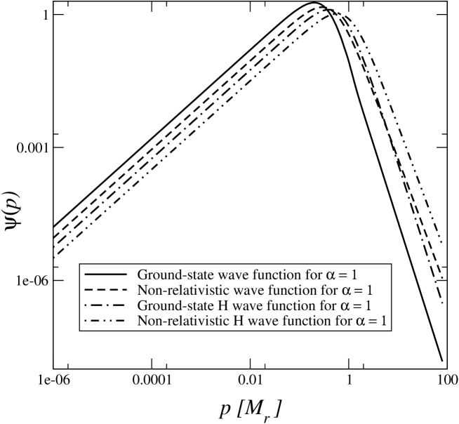
Figure 7: Double–logarithmic plot of the ground–state wave function for $\alpha=1$, compared to the non–relativistic results. The H wave function refers to a mass ratio $M_{A}/M_{B}$ as in the hydrogen atom, the other wave function is for equal masses.

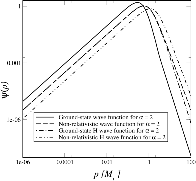
Figure 8: Plot of the ground–state wave function as in Fig. 7, for $\alpha=2$.

Adjusting the overall scale of the Coulomb wave functions cannot cure this problem.

Even though in the Coulomb basis the energy converges rapidly with the number of basis states, one can show that it does actually not converge to an eigenvalue of Eq. (35). Therefore, we have used a different basis, with a dependence on the two parameters $\beta$ and $\kappa$,

$$\phi_{n}(p)=\frac{\sqrt{3(2n+1)(2\beta-1)}}{\kappa^{3/2}\,[(p/\kappa)^{3}+1]^{\beta}}\,P_{n}\left(1-\frac{2}{[(p/\kappa)^{3}+1]^{2\beta-1}}\right)\>,$$ (63)

$P_{n}$ being a Legendre polynomial. This choice of basis leads to very satisfying results over a wide range of intermediate values of $\alpha$. For most purposes the values $\kappa=\alpha M_{r}$ and $\beta=3/2$ turned out to be sufficient. The wave functions are normalized to unity,

$$\int_{0}^{\infty}dp\,p^{2}\phi_{m}(p)\phi_{n}(p)=\delta_{mn}\>.$$ (64)

We have tested our results by comparing $H_{BW}\psi(p)$ to $E\psi(p)$ for the ground state, with the energy $E$ and wave function $\psi(p)$ determined as described above. The deviations are typically below one percent, which demonstrates that our numerical result for both the energy and the wave function constitutes an excellent approximation. For $\alpha=2$, the corresponding deviation in the case of the Coulomb basis is of the order of 25%. We have used up to 40 basis states, the changes in the deviation being minimal for more than 10 basis states. One can show that the difference $(H_{BW}-E)\psi(p)$ is orthogonal to the basis with an accuracy of $10^{-9}$ for our numerical integration, for both the Coulomb and the other basis. This also demonstrates that the problem with the Coulomb basis has nothing to do with the numerics.

The spectrum, as in most relativistic approaches, shows weaker binding than is expected from the extrapolation of the non–relativistic formula (see Figs. 9 and 10).

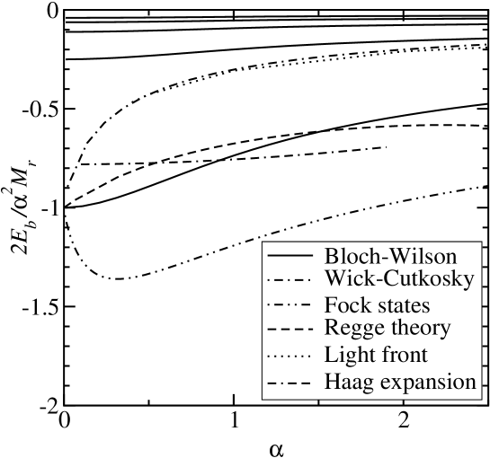
Figure 9: The spectrum of binding energies $E_{b}=E^{\prime}-M_{A}-M_{B}$ (cf. Eq. (35)) for $s$–states in the equal–mass case, compared to the ground state energies of the Wick-Cutkosky model [6], the Hamiltonian eigenvalue equation in a Fock space truncation [25], the Regge theory predictions [26], the light–front calculation [22], and the Haag expansion results [24] in their domain of validity.

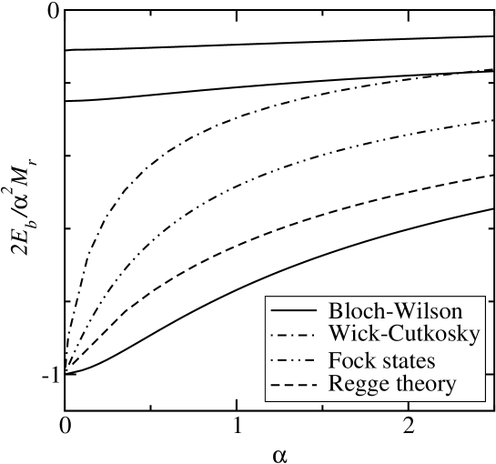
Figure 10: The spectrum of binding energies for $s$–states as in Fig. 9, for the hydrogen–masses case.

Consequently, the wave functions peak at a lower momentum. More interestingly, the power–law behavior of the high–momentum tail of the wave functions changes. Whilst the Coulomb wave functions behave like $p\psi(p)\sim p^{-3}$, the wave functions found here beyond the weak–coupling regime fall off more rapidly, with $p\psi(p)\sim p^{-3.5}$. The slope of the long–range tail in configuration space is unaltered by the relativistic corrections (see Figs. 7 and 8).

We have also made an attempt to visualize the non–local potential Eq. (37). Given a solution $\psi({\bf p})$ of the Schrödinger equation Eq. (35), one can define an “effective” local potential $V_{L}({\bf r})$ in position space by

$$V_{L}({\bf r})\psi({\bf r}) = \left[\int\frac{d^{3}p^{\prime}}{(2\pi)^{3}}\,V({\bf p},{\bf p}^{\prime})\psi({\bf p}^{\prime})\right]_{F.T.}$$ (65)

$$= \left[\left(E^{\prime}-\sqrt{M_{A}^{2}+{\bf p}^{2}}-\sqrt{M_{B}^{2}+{\bf p}^{2}}\right)\psi({\bf p})\right]_{F.T.}\>,$$

where $F.T.$ denotes the Fourier transform to position space. The definition Eq. (65) makes sense at least for the ground state, given that the latter has no nodes. Unfortunately, it is numerically very difficult to evaluate the expression Eq. (65) over the whole range of $\bf r$. However, we could determine that, somewhat unexpectedly, at the origin ${\bf r}=0$, $V_{L}$ tends towards finite values, numerically $V_{L}(0)=-15.0$ for $\alpha=1$ and $V_{L}(0)=-4.0$ for $\alpha=2$.

5 Discussion

The Bloch–Wilson Hamiltonian has a number of practical advantages over other relativistic approaches. Most notable is the absence of the energy eigenvalue in the potential part of the two–body bound–state equation. This has important computational advantages over formulations that have an energy–dependent integral kernel. We did not have to make any approximation for this result; it is a natural consequence of our approach. In the present formulation, the Hamiltonian is not Hermitian. Consequently, the left eigenstates are not identical to the right eigenstates, even though all eigenvalues turn out to be real. As a consequence of the similarity transformation back to the $H_{0}$–invariant subspace, the bound–state equation is expressed solely in terms of the two–particle wave function; all the internal workings of the interaction have gone in the Bloch–Wilson Hamiltonian.

To the present order in the perturbative expansion, all formally divergent contributions can be identified with proper on–shell Feynman diagrams, hence the renormalization procedure used in covariant Lagrangian perturbation theory can be applied to the effective Hamiltonian. This may not be possible at higher orders, nor can it be expected, of course, when a non–perturbative approach for the determination of the Bloch–Wilson Hamiltonian is chosen. In these cases, other and possibly not manifestly covariant renormalization procedures will have to be used. However, none of this is necessary in the present case. In particular, to the order considered the self–energy corrections merely serve to renormalize the masses.

Led by the results of the FSR approach [14, 31], it is nowadays believed that the Bethe–Salpeter equation suffers, apart from other unphysical features, also from a large underbinding. Our results lie closer to the non–relativistic values than the Bethe–Salpeter results and most other relativistic approaches (see Figs. 9 and 10), i.e., we find indeed a much stronger binding. Recently a discussion has emerged as to how the instability of the Wick–Cutkosky Hamiltonian could affect the bound state results [32]–[34]. At the present level of approximation, there seem to be no consequences of this unphysical feature of the model, however, how our approach can be extended to be sensitive to the instability is a topic for future research.

Not only is the non–relativistic limit properly recovered, as we were able to demonstrate both analytically and numerically, but also the one–body limit [30], where one particle becomes infinitely heavily, is consistent; the Schrödinger equation reduces to the equation for one particle interacting with a fixed source. Therefore, unlike the Bethe–Salpeter equation, the present approach can be used to study heavy–light systems, such as the hydrogen atom.

Finally, we comment on the invariance of the results under Lorentz boosts. In principle, bound states in a moving frame, i.e., with total momentum different from zero, can be calculated by solving the effective Schrödinger equation Eq. (32), and the results can be compared to the relativistic energy–momentum relation. At any rate, a perturbative Hamiltonian approach which by its very nature is not manifestly covariant, cannot be expected to maintain dynamical invariances, like boost invariance, exactly. As in the description of any non–perturbative phenomenon, some symmetries of the underlying theory will be violated at any level of approximation. A bound state in a moving frame will then slightly differ from a bound state at rest. This difference will become smaller with increasing order in the coupling constant to which the Bloch–Wilson Hamiltonian is calculated. However, we emphasize that in the present approach the expansion parameter is a Lorentz–invariant quantity, and the necessary renormalization is carried through in a covariant way, so that the violation of boost invariance might be expected to be small. To what extent boost invariance is actually broken at the present order and how much of it can be restored by calculating the Hamiltonian to a higher order is a topic of current research.

References

• [1] M. Gell-Mann and F. Low, Phys. Rev. 84 (1951) 350.
• [2] A.L. Fetter and J.D. Walecka, Quantum Theory of Many–Particle Systems (McGraw–Hill, New York, 1971).
• [3] A. Weber, in Particles and Fields — Seventh Mexican Workshop, eds. A. Ayala, G. Contreras, and G. Herrera, AIP Conference Proceedings 531 (American Institute of Physics, New York, 2000), hep–th/9911198.
• [4] C. Itzykson and J.–B. Zuber, Quantum Field Theory (McGraw–Hill, New York, 1980).
• [5] E.E. Salpeter and H.A. Bethe, Phys. Rev. 84 (1951) 1232.
• [6] N. Nakanishi, Prog. Phys. (Suppl.) 43 (1969) 1; ibid. 95 (1988) 1.
• [7] I.T. Todorov, Phys. Rev. D 3 (1971) 2351.
• [8] R. Blankenbecler and R. Sugar, Phys. Rev. 142 (1966) 1051.
• [9] A.A. Logunov and A.N. Tavkhelidze, Nuovo Cim. 29 (1963) 380.
• [10] F. Gross, Phys. Rev. 186 (1969) 1448.
• [11] D.R. Phillips and S.J. Wallace, Few Body Syst. 24 (1998) 175.
• [12] Yu.A. Simonov and J.A. Tjon, Ann. Phys. (N.Y.) 228 (1993) 1.
• [13] T. Nieuwenhuis, PhD thesis, University of Utrecht, The Netherlands, Oct. 1995.
• [14] T. Nieuwenhuis and J.A. Tjon, Phys. Rev. Lett. 77 (1996) 814.
• [15] S.J. Brodsky, H.-C. Pauli, and S.S. Pinsky, Phys. Rep. 301 (1998) 299.
• [16] J. Carbonell, B. Desplanques, V.A. Karmanov, and J.F. Mathiot, Phys. Rep. 300 (1998) 215.
• [17] S.J. Brodsky, J.R. Hiller, and G. McCartor, Phys. Rev. D 60 (1999) 054506.
• [18] R.J. Perry, Ann. Phys. (N.Y.) 232 (1994) 116.
• [19] E.L. Gubankova and F. Wegner, Phys. Rev. D 58 (1998) 025012.
• [20] T.S. Walhout, Phys. Rev. D 59 (1999) 065009.
• [21] C.R. Ji, Phys. Lett. B 322 (1994) 389.
• [22] M. Mangin-Brinet and J. Carbonell, Phys. Lett. B 474 (2000) 237.
• [23] J. Hansper, Phys. Rev. D 62 (2000) 056001.
• [24] O.W. Greenberg, R. Ray, and F. Schlumpf, Phys. Lett. B 353 (1995) 284.
• [25] N.E. Ligterink and B.L.G. Bakker, hep–ph/0010167.
• [26] A. Weber, J.C. López Vieyra, C.R. Stephens, S. Dilcher, and P.O. Hess, hep–th/0011280.
• [27] G.C. Wick, Phys. Rev. 96 (1954) 1124; R.E. Cutkosky, Phys. Rev. 96 (1954) 1135.
• [28] J. Goldstone, Proc. Roy. Soc. (London) A239 (1957) 267.
• [29] H.A. Bethe and E.E. Salpeter, Quantum mechanics of one– and two–electron atoms (Springer, Berlin, 1957).
• [30] F. Gross, Phys. Rev. C 26 (1982) 2203.
• [31] C. Savkli, J.A. Tjon, and F. Gross, Phys. Rev. C 60 (1999) 055210; Erratum ibid. C 61 (2000) 069901.
• [32] F. Gross, C. Savkli, and J. Tjon, nucl–th/0102041.
• [33] R. Rosenfelder and A.W. Schreiber, Phys. Rev. D 53 (1996) 3337, 3354.
• [34] S. Ahlig and R. Alkofer, Ann. Phys. (N.Y.) 275 (1999) 113.