UAB-FT-499

ABSTRACT

The phenomenology of the FLRW models with non-vanishing cosmological constant, $\lambda$, is briefly surveyed in the light of the recent astrophysical and cosmological observations. A subset of these $\lambda\neq 0$ models, which probably includes the world where we live, is singled out by the combined data from high redshift Type Ia supernovae, CMBR and the cosmic inventory of matter in our universe. The kinematical success of a non-vanishing $\lambda$, however, leaves open many dynamical questions in quantum field theory. A semiclassical renormalization group approach to $\lambda$ might perhaps shed some light on them. In this context, $\lambda$ is naturally non-zero simply because it is a running parameter.

1 Definition of $\lambda$ and a bit of history

In the following I will give a short review of some classic matters related to the impact of a non-vanishing cosmological constant on the kinematical evolution of the universe. Addressing the (much harder) issue of the cosmological constant problem in Quantum Field Theory, is not at all the main purpose of this note. Still, some of it will be sketched at the very end, hopefully in pedagogical terms. I will conclude with a remark on the potential relation of the cosmological constant to the renormalization group and the role played by the lightest degrees of freedom of our universe .

The cosmological constant (CC), $\lambda$, was first introduced by Einstein in 1917 [6] two years after he proposed the gravitational field equations without cosmological term [7]. In our conventions, the field equations in the presence of the cosmological constant read

$$G_{\mu\nu}+\lambda g_{\mu\nu}=-8\pi G_{N}T_{\mu\nu}\,,$$ (1)

where

$$G_{\mu\nu}\equiv R_{\mu\nu}-\frac{1}{2}g_{\mu\nu}R\,$$ (2)

is the so-called Einstein’s tensor, $T_{\mu\nu}$ is the energy-momentum tensor and $G_{N}$ is Newton’s constant. In Einstein’s words: “…we may add the fundamental tensor $g_{\mu\nu}$ multiplied by a universal constant, $-\lambda$ $\left[{}\right.$in his conventions$\left.{}\right]$, at present unknown, without destroying the general covariance… This field equation, with $\lambda$ sufficiently small, is in any case also compatible with the facts of experience derived from the solar system… That term is necessary only for the purpose of making possible a quasi-static distribution of matter, as required by the fact of the small velocities of the stars” [6].

Notice that the field equations (1) in the presence of $\lambda\neq 0$ can be obtained from the field equations for $\lambda=0$ with the simple substitution

$$T_{\mu\nu}\rightarrow\tilde{T}_{\mu\nu}=T_{\mu\nu}+\Lambda\,g_{\mu\nu}$$ (3)

We shall see later that the alternative CC parameter $\Lambda=\lambda/8\pi G_{N}$ plays a role on its own in that it represents a vacuum energy density. Then Eq. (1) can be cast as an effective set of vacuum equations

$$G_{\mu\nu}=-8\pi G_{N}\tilde{T}_{\mu\nu}\,.$$ (4)

Notice furthermore that $\lambda$ and $\Lambda$ are dimensionful scalar quantities. From the dimensions $\left[G_{N}\right]=E^{-2}$ and $\left[T_{\mu\nu}\right]=E^{4}$ in natural units, we have $\left[\lambda\right]=E^{2}$ and $\left[\Lambda\right]=E^{4}$. Nowadays the most stringent bounds (or actual estimations) on $\lambda$ come, rather than from our experience in the solar system, from cosmology (see later on), and entail

$$\lambda\stackrel{{\scriptstyle\scriptstyle<}}{{{}_{\sim}}}{\cal O}(10^{-84})\,GeV^{2}\Leftrightarrow\Lambda\stackrel{{\scriptstyle\scriptstyle<}}{{{}_{\sim}}}{\cal O}(10^{-47})\,GeV^{4}.$$ (5)

Since $\lambda$ is not dimensionless, we may assess the dramatic smallness of this number only by comparing it to another dimensionful quantity, such as e.g. the bound on the mass (squared) of the photon, from terrestrial measurements of the magnetic field:

$$m_{\gamma}^{2}\stackrel{{\scriptstyle\scriptstyle<}}{{{}_{\sim}}}{\cal O}(10^{-50})\,GeV^{2}\,.$$ (6)

In spite of our strong and unbreakable faith on the gauge dogma (which asserts that $m_{\gamma}=0$ exactly!) it turns out that we happen to know – by direct experimental knowledge – that the (queer and much more unfamiliar) parameter $\lambda$ is many orders of magnitude smaller than the most believed-to-be-zero physical parameter in the history of physical science: the photon mass.  How could anybody still doubt for a second that $\lambda$ should be zero too? All these compelling pieces of “evidence” notwithstanding, that might well not be the case after all!

It is perhaps useful to recall at this point that at the time when Einstein put forward his field equations with a non-vanishing cosmological term, astrophysicists did not even know that the stars that we may watch glowing beautifully in the firmament in a dark night are members of a very particular galaxy in the universe, our Milky Way Galaxy, which is just one among a hundred billions of them scattered amid the voids of the immense cosmos. Furthermore, from the historical point of view, we should emphasize that the cosmological constant was introduced by Einstein as a philosophical fiat, namely one that conformed with the classical trends of Western’s Philosophy. In view of the state of contemporary knowledge mentioned above, the idea of a static and ever unchanging cosmos was ingrained very profoundly in the current culture. Moreover, at the end of the last century it became notorious Mach’s conception (christened “Mach’s Principle” by Einstein himself [9]) according to which the inertia of a body is determined by the bulk matter distribution in the universe (Mach, 1893). Within this framework one is plausibly led to the conclusion that the universe had better be finite in space dimensions otherwise the bodies moving inside could not be affected by the overall matter content of the world. Another ingredient supporting the “necessity” for a finite universe was the so-called “Olbers paradox”, formulated in the middle of the nineteenth century, namely the fact that if the universe is infinite and homogeneous (filled with a constant average density of matter emitting a certain amount of radiation in all directions) we should observe a permanently bright sky due to the summing of all the luminous contributions of the uniform matter distribution in the world. In fact, although the intensity of the energy irradiated by the shell at distance $r$ dies off as $1/r^{2}$, the number of stars increases with $r^{3}$, so the net outcome is an ever increasing amount of radiant energy at all points of an infinite space. There wouldn’t be dark nights to see the stars!! Of course, according to our modern view, we know that there is no paradox at all. First, the number of stars within our physical horizon is, though enormous, finite; with an estimated total of $\sim 10^{11}$ galaxies, each containing an average of $\sim 10^{11}$stars, our universe contains, at most, $10^{22}$ shining suns “filling” the interstellar medium with an average density of scarcely a few protons per cubic meter. Second, the assumption that we receive that (approximately) constant amount of power from every shell is false. While it is reasonable to think that they do send a similar amount of electromagnetic energy, it is not true that we accumulate the total. To cure the disease, there is no need to assume a finite universe, for in an universe in expansion – even if infinitely large – the energy emitted from farther and farther shells becomes more and more red-shifted when it reaches the observer, and so the energy integral can be perfectly finite; in fact, it can be small enough to allow dark nights with crisp star views!

Hubble’s discovery (1929) of the recession of galaxies was the corner stone setting the experimental standpoint of modern cosmology. It instantly killed the necessity of a static universe – Einstein’s original universe– and, as quoted by Gamow [8], it made Einstein’s to exclaim that the introduction of the CC in his field equations was “the biggest blunder of my life”. As a matter of fact it was no blunder at all, for it could quite be that the CC is after all a physical reality – as I shall discuss in the next sections. Intriguingly enough, the possibility of a nonvanishing CC is perhaps the most profound legacy left over by the father of General Relativity.

2 The $\lambda$-force

$\lambda$ is indeed a constant independent of the chosen local inertial frame. The covariant derivative on both sides of Einstein’s Eqs. (1) is zero because of local conservation of energy-momentum ($\nabla^{\mu}T_{\mu\nu}=0$) and the automatic (Bianchi) identity $\nabla^{\mu}G_{\mu\nu}=0$ satisfied by the Einstein tensor. Therefore since $\nabla^{\mu}g_{\mu\nu}=0\Longrightarrow\nabla_{\mu}\lambda=0$ and so also $\partial_{\mu}\lambda=0\Longrightarrow\lambda$ is a constant scalar field –i.e. a parameter. To gather a physical intuition on the nature of $\lambda$ in Einstein’s equations let us interpret it in terms of forces. Consider the static gravitational field created by a source mass $M$ at the origin, with density $\rho_{M}=M\,\,\delta^{3}(r)$. For weak fields $g_{\mu\nu}\simeq\eta_{\mu\nu}$ is the usual Lorentz metric. We further assume a non-relativistic regime where $T_{00}\simeq\rho_{M}$ is just the matter density of the source. The $(\mu,\nu)=(0,0)$ component of Eq. (1) then reads $G_{00}+\lambda=-8\pi G_{N}\,\rho_{M}$ with $G_{00}=R_{00}-(1/2)R$. In the low-velocity (non-relativistic) case we also expect that $T_{ij}\ll T_{00}\,(i,j=1,2,3)$. This is equivalent to saying that we neglect pressure and stress as compared to matter density. Therefore, from (1) we are entitled to set $G_{ij}+\lambda g_{ij}\simeq 0$. This implies that $R_{ij}\simeq(1/2R-\lambda)g_{ij}$ and thus the curvature scalar boils down to $R=g^{\mu\nu}R_{\mu\nu}\simeq R_{00}+3(1/2R-\lambda)$, or $\ R\simeq-2R_{00}+6\lambda$. Substituting this back into the previous $(0,0)$ field equation we find $R_{00}-\lambda=-4\pi G_{N}\,\rho_{M}$. Also a very short computation confirms that, within our approximation, $R_{00}\simeq(-1/2)\nabla^{2}g_{00}$. Finally, recalling that Newton’s potential $\phi$ is related to the deviation of the $(0,0)$ component of the metric tensor from $\ \eta_{00}=1$ (through $\ g_{00}\simeq\ 1+2\phi$) we are led to the fundamental equation

$$\nabla^{2}\phi=4\pi G_{N}\left(\rho_{M}-\frac{\lambda}{4\pi G_{N}}\right)\,.$$ (7)

This is nothing but Poisson’s equation for the Newton potential with an additional term $-\lambda/4\pi G_{N}$ whose sign depends on that of $\lambda$. Thus if e.g. $\lambda>0$ the original gravitational field becomes diminished as though there were an additional repulsive interaction. In other words, the sign of the new force $F_{\lambda}$ has the sign of $\lambda$. These features are confirmed by explicitly solving Eq. (7):

$$\phi=-\frac{G_{N}\;M}{r}-\frac{1}{6}\lambda r^{2}$$ (8)

We are thus led to the expected gravitational potential plus a new contribution. The additional term is an  “harmonic oscillator” potential – repulsive for $\lambda>0$!. The corresponding force field on a test particle of mass $\mu$ ($\mathbf{g=F}/\mu$) reads

$${\bf g}=-\frac{G_{N}\;M}{r^{3}}{\bf r}+\frac{1}{3}\lambda{\bf r}$$ (9)

and contains an extra linear term with the aforementioned sign property.

3 Cosmologies with non-vanishing $\lambda$

We shall now show the impact of the $\lambda$-force in the cosmological scenario. We adopt the Cosmological Principle as the physical paradigm from where to build up our image of the universe. This principle asserts the isotropy (and a fortiori the homogeneity) of the universe in the large. In turn this leads to the Friedmann-Lemaître-Robertson-Walker (FLRW) type of cosmologies. If we concentrate on the matter-dominated (MD) era (more than $99.99\%$ of the universe lifetime) then the full spectrum of FLRW models follow from the basic Friedmann-Lemaître (FL) equation in the presence of a $\lambda$-term, namely

$$\dot{a}^{2}=\frac{C^{2}}{a}\,-k+\frac{\lambda}{3}\,a^{2}\equiv F(a)\,\,.$$ (10)

Here

$$C^{2}\equiv\left(8\,\pi\,G_{N}\,\,/3\right)\,\rho_{0}\,a_{0}^{3}$$ (11)

is a positive constant because its sign is that of $\rho_{0}=\rho_{M}(t_{0})$, the present energy density of matter. $F(a)\geq 0$ is, too, by construction a positive-definite function of the scale parameter $a(t)$. The value of the latter at present is denoted $a(t_{0})\equiv a_{0}$. Equation (10) follows from Einstein’s field equations (1) if one assumes a matter-energy distribution respecting the Cosmological Principle, therefore based on an isotropic energy-momentum tensor $T_{\mu\nu}$. However, by modeling the universe through an isotropic low-density medium, e.g. a perfect fluid sphere, pieced together in patches such that movements (e.g. expansion) are never relativistic in each piece, a Newtonian approach is possible. Then the energy conservation law –including the $\lambda$-term from (8)– for a patch of mass $\mu$ sitting at $a=a(t)$ reads

$$\frac{1}{2}\,\mu\,\dot{a}^{2}-\rho\left(\frac{4}{3}\pi\,a^{3}\right)\frac{G_{N}\,\mu}{a}-\frac{1}{6}\,\lambda\,\mu\,a^{2}\,=E\,.$$ (12)

Here $t$ is the cosmological proper time, namely the time measured by every observer that accompanies the mean motion of the uniform matter distribution in the universe, modeled as a perfect fluid. The existence of this cosmic time is a consequence of the Cosmological Principle. In fact, the latter requires that every cosmological parameter and field of the “fluid universe”, be at most a function of the cosmological proper time, $f=f(t)$, and so $f$ must be homogeneous and isotropic in space coordinates. In this respect I should point out that the Cosmological Principle does not preclude the possibility that the CC could be, as the scale factor itself, a function of the cosmic time: $\lambda=\lambda(t)$. From the point of view of the co-moving observer, this $t$-dependent “cosmological constant” is to be interpreted as an additional gravitational source beyond the original $T_{\mu\nu}$, in the manner of eq. (3). Therefore, the total source is

$$\widetilde{T}_{\mu\nu}=T_{\mu\nu}+\frac{\lambda(t)}{8\pi G_{N}}\,g_{\mu\nu}=T_{\mu\nu}+\Lambda(t)\,g_{\mu\nu}$$ (13)

The difference with respect to eq.(3) is that in the present instance it is the total $\widetilde{T}_{\mu\nu}$ that is conserved, not the original $T_{\mu\nu}$. Of course this is required by the Bianchi identity satisfied by the Einstein tensor $G_{\mu\nu}$, as explained at the beginning of Section 2. The case of a variable $\lambda=\lambda(t)$, however, will not be pursued here anymore. Let us just mention that it is at the heart of the so-called “quintessence” models [10].

Next consider the equation of continuity of our perfect fluid medium (in the MD era, where pressure and radiation density are negligibles in front of matter density $\rho_{M}$). Since $|{\bf r}|=a$ and $|\dot{\bf r}|=\dot{a}$ we have $\dot{\bf r}=\dot{a}\,({\bf r}/a)=H\,{\bf r}$ and hence the equation of continuity of our non-relativistic fluid model yields

$$0=\frac{\partial\rho_{M}}{\partial t}+{\bf\nabla}\cdot(\rho_{M}\,{\bf\dot{r}})=\dot{\rho}_{M}+3\,H\,\rho_{M}$$

$$\Rightarrow\,\frac{d\rho_{M}}{\rho_{M}}+3\,\frac{da}{a}=0\,,$$ (14)

where we notice that, by virtue of the Cosmological Principle, $\rho_{M}(t)$ can only be a function of $t$ at most. Therefore, Eq. (14) is trivially integrated to give $\rho_{M}(t)\,a^{3}(t)=\rho_{0}\,a_{0}^{3}=\mathrm{const.}$. We may now substitute this first integral on Eq.(12) to eliminate the density. Moreover, in our Newtonian picture the Gaussian curvature constant $k$ of the $3$-space sections of the space-time is recovered through the prescription

$$k=-{\frac{E}{|E|}}\equiv\left\{\begin{array}[c]{lll}-1&\mbox{if $E>0$\ (open)}&\\ 0&\mbox{if $E=0$\ (flat)}&\\ +1&\mbox{if $E<0$\ (closed)}&\end{array}\right.\,.$$ (15)

Of course we are free to rescale the scale factor e.g. $a\rightarrow(\sqrt{2\left|E\right|/\mu})\,a$. In doing this Eq.(12) finally transforms into the FL equation (10).

A graphic summary of the FLRW cosmologies is sketched in Figs. 1-2. We have divided them into three classes: Class I ($k=-1$), Class II ($k=0$) and Class III ($k=+1$), and each class subdivides into models depending on the value of the CC. The analysis of these models is in principle not difficult as the differential equation (10) can be integrated by quadrature,

$$t_{0}-t=\int_{a(t)}^{a_{0}}\frac{da}{\sqrt{F(a)}}\,.$$ (16)

From here one obtains $t=t(a)$ and upon inverting one gets $a=a(t)$. Unfortunately, neither of the last two operations can be performed analytically in the general case. For $\lambda=0$ (and any $k$) or for $k=0$ (and any $\lambda$) the integral (16) can be done explicitly, but for $k=\pm 1$ and $\lambda\neq 0$ it leads to an elliptic function and so numerical integration is required for an accurate quantitative description. Nonetheless the qualitative traits of the resulting function $a=a(t)$, and so the various types of FLRW universes, can be pinned down analytically in all cases without need of an explicit numerical analysis.

But before embarking us on further discussions it is convenient to define the canonical cosmological parameters at the present time. They are defined to be the present energy density of matter and cosmological constant in units of the critical density now:

$$\Omega_{M}\equiv\frac{\rho_{0}}{\rho_{0}^{c}}\,,\ \ \ \Omega_{\Lambda}\equiv\frac{\Lambda}{\rho_{0}^{c}}=\frac{\lambda}{3\,H_{0}^{2}}\,,$$ (17)

$$\rho^{c}_{0}\equiv\frac{3\,H_{0}^{2}}{8\,\pi\,G_{N}}=\left(3.0\,\sqrt{h_{0}}\times 10^{-3}\,eV\right)^{4}\,.$$ (18)

Here the dimensionless number $h_{0}\sim 0.65\pm 0.1$ [11] sets the typical range for today’s value of Hubble’s “constant”

$$H_{0}\equiv\left({\dot{a}\over a}\right)_{0}=100\;{Km/sec\over Mpc}\;h_{0}\,.$$ (19)

From these parameters the FL Eq.(10) can be trivially cast in the form of an exact sum rule for the present time:

$$\Omega_{M}+\Omega_{\Lambda}+\Omega_{K}=1\,,$$ (20)

where $\Omega_{K}=-k/a_{0}^{2}\,H_{0}^{2}$ is the cosmological curvature parameter, which is seen to be dependent of the other two previously defined. In the absence of $\lambda$ the resulting cosmological models are extremely simple: Cf. Models I2, II2 and IIIb in Figs. 1-2. However, these are just very particular cases of the full collection of $14$ FLRW models with $\lambda\neq 0$ displayed in these figures. We remark that FLRW models with vanishing CC have the property that the universe is spatially open ($k=-1$), closed ($k=+1$) or flat –i.e. Euclidean ($k=0$)– if and only if it expands forever, ultimately re-collapses (into a “Big Crunch” point) or expands just up to the border between expansion and re-collapse, respectively. Nevertheless such a one-to-one correspondence between the ultimate destiny of the universe and the topological structure of its associated $3$-space no longer holds when $\lambda\neq 0$. For example, a spatially closed universe (hence a compact one) with non-vanishing CC could well be one that expands forever (Fig. 2), and a spatially open or flat universe with non-vanishing CC could ultimately recollapse (Fig. 1).

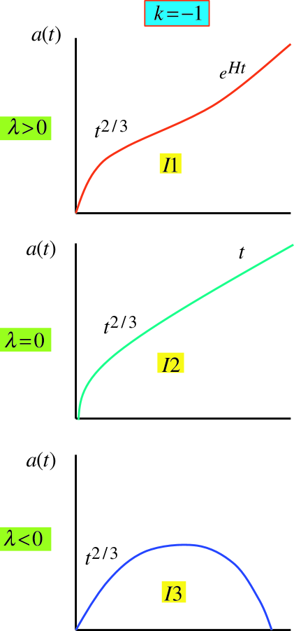
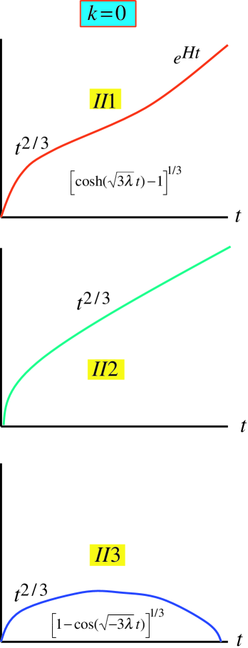
Figure 1: The Class I and Class II FLRW models. Model II1 is both theoretically and experimentally favored. Model II2 is the Einstein-de Sitter model.

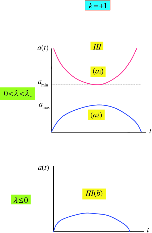
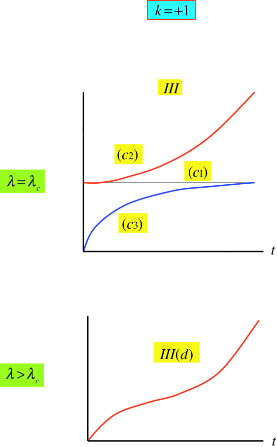
Figure 2: The rich Class III of FLRW models. In particular, Model III(c1) is Einstein’s static model, Model III(c2) is the Eddington-Lemaître model and Model III(d) is similar to Model II1, except that $k=+1$. It could also be a favored case, see Fig. 3a.

In the following I wish to comment a bit more on a few of the FLRW models in Figs.1-2. Model II2 is a $\lambda=0$ universe of particular historical interest, viz. the Einstein-de Sitter (EdS) model from 1932, just devised by these authors after Einstein abjured in 1931 the creature he had engendered fourteen years before: the CC itself! The EdS model is the simplest FLRW cosmological model accounting for the observed expansion. However, it is a “critical model”, namely the density of matter is exactly equal to the critical density, $\rho_{0}=\rho_{0}^{c}$ (equivalently, $\Omega_{M}=1$), and for this reason eq.(20) trivially implies that it is a spatially flat universe with vanishing CC. The EdS model solves in a very simple analytical form upon integrating Eq.(16) with $k=0$ and $\lambda=0$, with the result: $a^{3}(t)=(3\,C\,t/2)^{2}$. Notice that the behavior $a(t)\propto t^{2/3}$, valid for all $t$ only in this model, is nevertheless characteristic of all the FLRW models with initial singularity (“Big Bang”) when we approach $t\rightarrow 0$ within the MD epoch, see Figs. 1-2. Paradoxically, the EdS model is nowadays excluded (see Fig. 3a) as it gives a really poor man fit to the combined data from high redshift Type Ia supernovae [12], the temperature anisotropies in the cosmic microwave background radiation (CMBR) [11, 14, 15] and the dynamical observation of clustered matter [14]. At the end of the day the (formerly abhorred) CC is back again, and with renewed momentum! Models with positive CC are singled out by observation at the $99\%$ C.L.!

Particularly favored is Model II1 (Cf. Fig. 1). In this case one can also derive from (16) the exact analytical evolution of the scale factor for all $t$. It involves a hyperbolic cosine function whose asymptotic (exponential) behavior matches that of the closed model I1. The result is

$$a^{3}(t)=\frac{3\,C^{2}}{2\,\lambda}\,\ \left[\cosh\left(\sqrt{3\,\lambda}\,t\right)-1\right]\,.$$ (21)

For convenience I have normalized this solution such that $a(0)=0$. We verify that $a(t)\sim\exp{(H_{\lambda}\,t)}$ for $t\rightarrow\infty$, where $H_{\lambda}\equiv\sqrt{\lambda/3}$ is Hubble’s constant in the de Sitter space.

Class III is the one with the richest spectrum of models, see Fig.  2. There is a critical value $\lambda_{c}\equiv 4/(9\,C^{4})>0$ obtained from requiring that the discriminant of the cubic equation $F(a)=0$ is zero in order to guarantee a double (positive) real root $a=a_{c}\equiv 3C^{2}/2=1/\sqrt{\lambda_{c}}$. The subclasses are easily identified. If $0<\lambda<\lambda_{c}$ (see Fig.2, up-left), then there is an excluded segment $a_{\mathrm{max}}<a(t)<a_{\mathrm{min}}$ in which $F(a)<0$. There are two allowed models of this sort depending on whether $0\leq a(t)\leq a_{\mathrm{max}}$ –Model III(a2)– or $a(t)>a_{\mathrm{min}}$ –Model III(a1). Notice that the former model is oscillatory whereas the latter (“bouncing universe”) has the curious property that it has no $t=0$ singularity. In fact, Model III(a1) contracts exponentially from infinity and then expands back towards the same place at the same pace. As for the two cases $\lambda<0$ and $\lambda=0$ in Fig. 2 (down-left), they are both dubbed Model III(b) and are similar to the oscillatory models discussed before. Worth noticing are the three subclasses IIIc ($\lambda=\lambda_{c}$) in Fig. 2 (up-right). The remarkable thing about Model III(c1) is that it is just the original static Einstein model at fixed $a=a_{c}$. Though static, it corresponds to an unstable fixed point of the FL differential equation (10). This was already noticed by Eddington on simple physical grounds: if for some reason this universe would expand slightly, this would diminish the gravitational attraction but at the same time would enhance the repulsive $\lambda$-force ($\lambda_{c}>0$!)  because the latter is larger the larger is the separation between particles. As a result the original “seed expansion”, no matter how small it is, would destabilize the universe into a “runaway expansion”. Similarly, an initial “seed contraction” would cause the universe to shrink indefinitely. Mathematically, by perturbing the solution one obtains, in one case, a non-singular model – Model III(c2)– which starts at $a=a_{c}$ and then evolves exponentially up to infinity (the so-called Eddington-Lemaître model), and in the other case a model – Model III(c3)– which starts at the singularity $a=0$ and then creeps up asymptotically towards $a=a_{c}$. Finally, for $\lambda>\lambda_{c}$ one obtains Model III(d) in Fig. 2 (down-right) which is similar to models I1 and II1. Interestingly enough, if Model III(d) is such that $\lambda$ is only slightly larger than $\lambda_{c}$, then there appears an approximately flat region in the middle of the curve and we obtain a quasi-Einstenian model in which $a(t)$ loiters a long while around $a=a_{c}$ before the eventual (exponential) de Sitter’s phase takes over. It follows that, for an appropriate choice of $\lambda>0$, such a “Lemaître’s hesitation universe” can be made arbitrarily old!

4 The universe where we live

After this short review of the FLRW cosmologies with non-vanishing CC we are now in position to discriminate between the most favored models according to the latest experimental observations. As already mentioned, the flat and critical ($\Omega_{M}=1$) EdS model (Model II2), which was a preferred cosmological scenario for about 40 years (viz. through a period mediating from 1932 until the $70s$), is no longer favored. As a matter of fact it is deadly ruled out by the combined data (Cf. Fig. 3a). Although the EdS model is a prototype dark matter model, it turns out to predict too much dark stuff!! For, as can be seen in Fig. 3a, the most recent galaxy clustering observations seem to point towards a low-density universe ($\Omega_{M}<1$). This fact together with the supernova data insisting on a positive CC of the order (actually larger than that) of the matter density gives a final verdict excluding the flat EdS universe. There is, however, another flat model, although certainly a non-critical one, in our list of Sec. 3, which is nowadays a most cherished candidate for a viable model of our universe: Model II1 in Fig. 2. This FLRW model is a flat universe with positive CC ($k=0\,,\lambda>0$). It is strongly highlighted both on theoretical grounds (by the inflationary paradigm) and experimentally – because it is compatible with the supernovae data, the astrophysical inventory of clustered matter, the revised age determinations of the globular clusters (the oldest objects known in our galaxy) and also with the precise measurements of the temperature anisotropies in the CMBR [11]. Thus at present we have a consistent solution to the various “age problems” plaguing this field in the past. To fix this conundrum it helps to have a non-vanishing and positive CC, but also the fact that the revised ages of the globular clusters are smaller than previously thought  [16].

	(a)	(b)

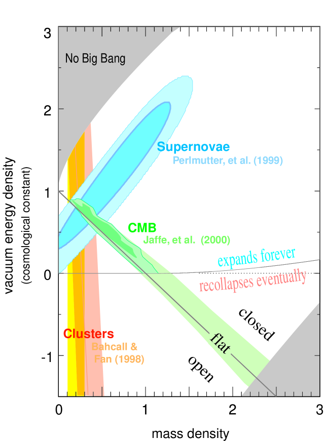
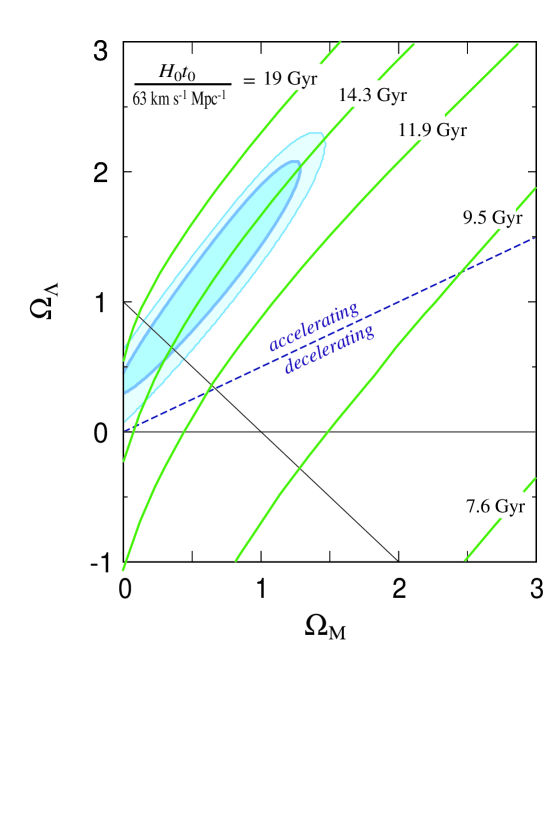
Figure 3: (a) Combined data from high redshift Type Ia supernovae, CMBR and clustered matter observations plotted in the plane $(\Omega_{M},\Omega_{\Lambda})$ defined by the mass density and the vacuum density (CC) in units of the critical density. It is seen that the $\lambda>0$ FLRW cosmological models with $0<\Omega_{M}<\Omega_{\Lambda}$ expanding forever are clearly favored; (b) Type Ia supernovae data as in (a) showing that the preferred model is an accelerating universe about $14-15\,Gyrs$ old. See Refs. [12, 13, 14, 15].

The best candidate model universe, Model II1, is singled out as a crossover area in Fig. 3a around the flat space point $\Omega_{M}\simeq 0.28,\,\Omega_{\Lambda}\simeq+\,0.72$. In the vicinity of this point the supernovae data, the CMBR data and the dynamical counting of clustered matter in the universe are best met than in any other region of the $(\Omega_{M},\Omega_{\Lambda})$ plane. Notwithstanding, we should emphasize that the data just off the $k=0\,,\lambda>0$ line ($\Omega_{M}+\Omega_{\Lambda}=1$) in Fig. 3a is tilted into the domain of closed, low-mass, universes with positive CC. Therefore, from the strict point of view of the experimental observation, a closed universe of the Type III(d) in Fig. 2 cannot be excluded in spite of all the theoretical prejudices that we might have in mind!

Worth noticing is that none of the non-singular (i.e. no Big Bang) FLRW cosmological models is singled out by supernovae data and CMBR (Cf. Fig.  3). For example, the shaded set of points on the left upper corner of Fig. 3a correspond to “bouncing universes” – see Model III(a1) in Fig. 2 – namely those that shrink down to a minimum from infinity and then recede to that point in the future. These universes are seen to be the oldest ones (Cf. Fig. 3b) but cannot be accepted, and not only because they are incompatible with supernovae data. But also because it can be proven that at the point of highest shrinking the density parameter is bounded from above by a too small quantity

$$\Omega_{M}\leq\frac{2}{z_{\rm max}^{2}(z_{\rm max}+3)}\stackrel{{\scriptstyle\scriptstyle<}}{{{}_{\sim}}}0.01$$ (22)

whose numerical value reflects the fact that we have already observed objects (e.g. quasars) with redshifts $z\stackrel{{\scriptstyle\scriptstyle>}}{{{}_{\sim}}}5$ – or even higher according to very recent, preliminary, data on remote proto-galaxies. On the other hand, the formerly (very famous) Lemaître “loitering universes” lying on the border line around the set of “bouncing universes” (upper left corner of Fig.3a) are seen to be also excluded. As for the shaded set of points on the down-right corner of Fig. 3a, it is also ruled out (see Fig. 3b) on the grounds that these universes are too young ($t_{0}<9\,Gyr$) so that the oldest heavy elements would not have had time to form. In short, in the light of the present cosmological observations the existence of a tiny $\lambda>0$ does help in an essential way to reconcile the age of the universe with the age of the oldest (known) objects living inside it and in general to obtain an overall picture which is in harmony with the experimental reckoning of cosmic matter and relic radiation.

5 Cosmological Constant and Particle Physics

5.1 The CC problem in the SM

In spite of the goodness of a non-vanishing CC from the point of view of cosmological kinematics, the existence of a tiny positive cosmological constant poses serious dynamical questions that go to the heart of Theoretical Elementary Particle Physics inasmuch as it is based on Quantum Field Theory (QFT). For instance, there are enormous contributions to the CC in the Standard Model (SM) coming from the spontaneous breaking of the electroweak symmetry, i.e. from the vacuum expectation value of the Higgs potential. If we call $\Lambda_{ind}$ the (overall) induced vacuum energy density from QFT, then the total energy-momentum tensor gets an additional vacuum contribution: $T_{\mu\nu}\rightarrow T_{\mu\nu}+<0|T_{\mu\nu}|0>$ in which, by Lorentz covariance, $<0|T_{\mu\nu}|0>=g_{\mu\nu}\,\Lambda_{ind}$ (Cf. Eq.(3) ) Therefore, in the semiclassical approach, the total effective cosmological constant entering Einstein’s equations (1) reads

$$\lambda_{eff}=\lambda+8\,\pi\,G_{N}\,\Lambda_{ind}\equiv\lambda+\lambda_{ind}\,.$$ (23)

Of course it is this effective quantity (the sum of the “vacuum CC” and the “induced CC”) what the supernovae and CMBR measurements must have pinned down. Then the “cosmological constant problem” [2] appears in the context of the SM when one considers the contribution from the QCD and electroweak vacuum energies to $\lambda_{ind}$ in Eq.(23). Let us focus on the electroweak part only. The Higgs potential of the SM reads

$$V_{cl}=-\frac{1}{2}m^{2}\phi^{2}+\frac{f}{8}\phi^{4}.$$ (24)

Let $v$ be the vacuum expectation value (VEV) of $\phi$, namely the value where $V_{cl}$ becomes minimum. Then, shifting the original field $\phi\rightarrow H^{0}+v$ such that the physical scalar field $H^{0}$ has zero VEV, one obtains the physical mass of the Higgs boson: $M_{H}=\sqrt{2}\;m$. At the minimum of the potential (24):

$$\phi=\sqrt{\frac{2m^{2}}{f}}=v\,\,\,\,\,\,{\rm and}\,\,\,\,\,\,\,f=\frac{M_{H}^{2}}{v^{2}}\,.$$ (25)

From (25) one obtains the following value for the potential, at the tree-level, that goes over to the induced CC:

$$\Lambda_{ind}=<V_{cl}>=-\frac{m^{4}}{2f}\,.$$ (26)

If we apply the current numerical bound $\,M_{H}\stackrel{{\scriptstyle\scriptstyle>}}{{{}_{\sim}}}115\,GeV$ from LEP II, then the corresponding value $\left|\Lambda_{ind}\right|\simeq 1.0\times 10^{8}\,GeV^{4}$ is $55$ orders of magnitude greater than the observed CC from the supernovae. (Recall that $\Lambda_{ph}\sim 10^{-47}GeV^{4}$ –Cf. Eq.(5)– as it follows from using the favored value $\Omega_{\Lambda}\sim 0.7$ mentioned in Sec. 4, and $\rho_{0}^{c}$ given in Eq.(18)). Clearly, unless we fine tune the original $\lambda$ term (or “vacuum CC term”) on the RHS of Eq.(23) with a precision of $55$ decimal places we are in trouble. But of course, even if doing this fantastic fine tuning, which is technically possible in principle, we are still in trouble because it has to be repeated order by order in perturbation theory, and this is certainly untenable.

5.2 A remark on a renormalization group approach

Many theoretical ideas have been proposed to solve this ever-growing conundrum  [2]. However, for lack of space, I will only mention the possibility, recently put forward in Refs.[4, 5], that the CC has to be treated as a running parameter in a semiclassical formulation of the gravitational field equations. This way does not provide the fundamental solution of the CC problem either. Nevertheless it helps in better understanding the problem and (maybe even more important) in drawing some physical consequences out of it. The basic idea is that in QFT the vacuum action is subject to renormalization and to the renormalization group running. At any given energy scale $\mu$ the CC will have a different value $\Lambda(\mu)$ driven by a renormalization group equation (RGE) and boundary conditions. Consequently, the “cosmological constant” is not a constant, still less should be zero. In this approach one can derive the contributions from the light particles to the running of the cosmological and gravitational constants in the SM, starting from the cosmic scale up to the Fermi scale. In particular, near the present cosmic scale $\mu\sim\mu_{c}$ (see below) one can show that the full CC (induced plus vacuum parts) obeys a RGE driven by the lightest degrees of freedom (d.o.f.) available in the universe. The final form of the RGE for the physical CC depends not only on the RGE for the vacuum term, but also on the RGE for the induced term, i.e. the RGE for the VEV of the effective potential, eq. (26). However, the latter is already determined by the RGE of the SM couplings and parameters. In the general case, the relevant equation is given in  [5], but at the present epoch of our universe it just boils down to  [4]

$$(4\pi)^{2}\frac{d\Lambda_{ph}}{dt}\,=\frac{1}{2}\,m_{S}^{4}\,-\,4\,\sum_{i}\,m_{\nu_{i}}^{4}\,.$$ (27)

Here $S$ is a very light scalar field (which we may call “Cosmon”), whose mass $m_{S}$ is a few times the average mass of the lightest neutrinos $m_{j}$  [20]. Typically these may include the electron neutrino and a sterile neutrino. Let us just consider the electron type; then $m_{S}\stackrel{{\scriptstyle\scriptstyle>}}{{{}_{\sim}}}4\,m_{\nu_{e}}$ [4]. Thanks to the scalar nature of the Cosmon, the running can be such that if one starts with zero CC at the very far infrared (IR) epoch of the universe, a positive CC can be generated at the present time and with the right order of magnitude according to the supernovae experiments. In addition, this new point of view helps to get a grasp to the so-called “cosmic coincidence cosmological constant problem”, namely the problem of why the measured CC just happens to be of the order of the present day matter density. This is tantamount to asking why the CC starts to dominate the energy density of the universe at the epoch of structure formation. Of course one can invoke “anthropic considerations” [3], but from our point of view [5] the value of $\Lambda$ at present is obtained from RG arguments alone once the initial conditions are fixed at some renormalization point. The latter can typically be the very far IR scale, $\mu_{IR}$, where the value of the CC can in principle be whatever. The scale $\mu_{IR}$ is the “ultimate energy scale” down the present day cosmic scale $\mu_{c}$ where no active d.o.f. are available – from the RG point of view. It is reasonable to associate the cosmic scale at present with a quantity of order of (Cf. eq.(18))

$$\mu_{c}\sim\left(\rho_{0}^{c}\right)^{1/4}=3.0\,\sqrt{h_{0}}\times 10^{-3}\,eV\,.$$ (28)

This scale is near the value of the lightest neutrino masses invoked to solve the various neutrino puzzles [20]. Therefore, one can arrange for the Cosmon and the lightest neutrino to be the only RG-active d.o.f. at present, as explained above. Then the RGE for the physical CC in the segment from the far IR up to the scale of the next-to-lightest-neutrino, say $\nu_{\mu}$, is given as follows:

$$(4\pi)^{2}\frac{d\Lambda_{ph}}{dt}\,=\left\{\begin{array}[]{ccc}\frac{1}{2}\,m_{S}^{4}\,-\,4\,m_{\nu_{e}}^{4}&\mbox{ $(m_{\nu_{\mu}}>\mu>m_{S}>m_{\nu_{e}})$\ }&\\ ?&\mbox{ $(\mu_{IR}\leq\mu<m_{\nu_{e}})$\ }&\end{array}\right.\,.$$ (29)

Here we have normalized $t$ such that $t=\ln(\mu/\mu_{IR})$. In general we can expect $\mu_{IR}\ll\mu_{c}$. The value $\Lambda_{ph}(IR)$ of the CC in this “ultimate” energy scale (where no active d.o.f. remain) can be zero or not, but in any case we do not know the running near it because we ignore if there are extra (ultralight) d.o.f. in its immediate vicinity. If, however, one assumes (perhaps by invoking some string symmetry [3]) that $\Lambda(\mu_{IR})=0$, and that there are no other d.o.f. than those already considered, then the value $\Lambda_{ph}(\mu)$ at any scale $\mu>\mu_{IR}$ becomes determined, and in particular also the value $\Lambda_{ph}(\mu_{c})$ at the present cosmic scale $\mu_{c}$. In this case we have the following interesting situation. On the one hand $\Lambda_{ph}(\mu_{c})$ is just obtained from the RGE (29), implying that the present day physical value of the CC is, roughly, $\Lambda_{ph}\equiv\Lambda_{ph}(\mu_{c})\sim m_{S}^{4}\stackrel{{\scriptstyle\scriptstyle>}}{{{}_{\sim}}}m_{\nu_{e}}^{4}$. And, on the other hand, we have $\rho_{0}^{c}\sim\left((2-3)\times 10^{-3}\,eV\right)^{4}$, and this number happens to be of order $m_{\nu_{e}}^{4}$ – and of course of order $m_{S}^{4}$. Hence one obtains the desired relation $\Lambda_{ph}\sim\rho_{0}$, which “explains” the supernovae data and the “cosmic coincidence”. It should be pointed out that, within our framework, this relation is equally valid now as it was in the epoch of structure formation. This is because, as mentioned above, the next-to-lightest d.o.f. ready to contribute to the RHS of the RGE (27) is the muon (and tau) neutrino, which in the canonical solutions to the neutrino puzzles [20] are nearly degenerate and of order $1\,eV$. Therefore, since they are three orders of magnitude heavier than the lightest neutrino, they should have already decoupled from the RG evolution of the physical CC at the time of structure formation, and so eq.(29) still applies at that time. This justifies our contention. Finally, it is worth mentioning that when extrapolating the running of the CC at higher energies in this framework (e.g. energies of order of the electron mass, in which the electron becomes an RG-active d.o.f.) one can show that the scaling dependences of the cosmological (and gravitational) constants do not spoil primordial nucleosynthesis, a quite rewarding result  [5].

Acknowledgments: I am grateful to the organizers for the kind invitation and the nice atmosphere met in Sant Feliu de Guíxols. I thank S. Bludman,  M.C. González-García, A. Goobar, I.L. Shapiro and J.W.F. Valle for useful conversations. I thank also A. Goobar for providing me Fig. 3a. This work has been supported in part by CICYT under project No. AEN99-0766.

References

- [1] J. Solà, Introduction to the cosmological constant in Einstein’s equations, preprint UAB-FT, in preparation.
- [2] S. Weinberg, Rev. Mod. Phys. 61 (1989) 1, and references therein.
- [3] E. Witten, The cosmological constant from the viewpoint of string theory, talk in: Dark Matter 2000, Marina del Rey, C.A., February, 2000 [hep-ph/0002297]; ibid. S. Weinberg, The cosmological constant problems [astro-ph/0005265].
- [4] I.L. Shapiro, J. Solà, Phys. Lett. 475 B (2000) 236.
- [5] I.L. Shapiro, J. Solà, Scaling behavior of the cosmological constant: Interface between Quantum Field Theory and Cosmology, preprint UAB-FT-490 [hep-th/0012227].
- [6] A. Einstein, Sitzber. Preuss. Akad. Wiss. Berlin (1917) 142.
- [7] A. Einstein, Sitzber. Preuss. Akad. Wiss. Berlin (1915) 315.
- [8] G. Gamow, My World Line (Viking Press, New York, 1970).
- [9] A. Einstein, Ph. Z. 17 (1916) 101-104.
- [10] S. Bludman, these proceedings.
- [11] J.I. Silk, these proceedings.
- [12] S. Perlmutter et al., Astrophys. J. 517 (1999) 565; A.G. Riess et al., Astrophys. J. 116 (1998) 1009.
- [13] A. Goobar, these proceedings.
- [14] A.H. Jaffe et al., astro-ph/0007333; N.A. Bahcall and X. Fan, astro-ph/9804082.
- [15] P. de Bernardis et al., Nature 404 (2000) 955 .
- [16] B. Chaboyer et al., Astrophys. J. 494 (1998) 96.
- [17] R.D. Peccei, J. Solà and C. Wetterich, Phys. Lett. B 195 (1987) 183.
- [18] C. Wetterich, Nucl. Phys. B 302 (1987) 645 and 668.
- [19] J. Solà, Phys. Lett. B 228 (1989) 317; ibid. Int. J. of Mod. Phys. A 5 (1990) 4225.
- [20] M. C. Gonzalez-Garcia, M. Maltoni, C. Pena-Garay and J.F.W. Valle, Global three-neutrino oscillation analysis of neutrino data [hep-ph/0009350], to appear in PRD. See also M. C. Gonzalez-Garcia, C. Pena-Garay and J.F.W. Valle in these proceedings.