LU TP 01-01

IPNO-DR/01-003

hep-ph/0101127

January 2001

QCD Isospin Breaking in Meson Masses, Decay Constants and Quark Mass Ratios
G. Amoros^a,b, J. Bijnens^a and P. Talavera^c

^a Department of Theoretical Physics 2, Lund University,

Sölvegatan 14A, S22362 Lund, Sweden

^b Departament de Física Teòrica, IFIC, Universitat de València-CSIC,

Apt. Correus 22085, E-46071 València, Spain

^cGroupe de Physique Théorique, Institut de Physique Nucléaire,

Université Paris Sud, F-91406 Orsay Cedex, France

The procedure to calculate masses and matrix-elements in the presence of mixing of the basis states is explained in detail. We then apply this procedure to the two-loop calculation in Chiral Perturbation Theory of pseudoscalar masses and decay constants including quark mass isospin breaking. These results are used to update our analysis of $K_{\ell 4}$ done previously and obtain a value of $m_{u}/m_{d}$ in addition to values for the low-energy-constants $L_{i}^{r}$.

PACS numbers: 12.15.Ff,13.20.Eb, 11.30.Rd, 12.39.Fe

1 Introduction

Experiments in low-energy QCD are becoming more and more precise. It is therefore needed that theoretical calculations are performed to similar accuracy. In the purely mesonic sector the low-energy effective theory of QCD is known as an effective theory in terms of pseudo-scalar mesons only. It is known as Chiral Perturbation Theory (CHPT) and was put on a solid theoretical basis in [1]. In the two-flavour sector calculations to two-loop order are now customary. In our earlier work [2, 3], where also references to other calculations can be found, we have performed the main calculations in the three flavour sector also to two loops in the isospin symmetric approximation.

One of the remaining uncertainties was the importance of isospin breaking effects. Basically in our previous work and many other theoretical calculations isospin breaking was only included by guessing its effect and putting it in the uncertainty of the final result. An example where we definitely need to go beyond this is in the use of $K_{\ell 3}$ form-factors [4] to extract an accurate value of the $|\,V_{us}\,|$ CKM matrix-element. Here we take a first step in that we evaluate within CHPT the strong isospin breaking in masses and decay constants to next-to-next-to-leading order.

This work serves two purposes: it checks the dependence on isospin breaking of the determination of the CHPT low-energy constants (LEC’s) at ${\cal O}(p^{4})$ performed in our earlier work [2, 3] and allows us to extract information on the quark mass ratio $m_{u}/m_{d}$. The latter is one of the fundamental input parameters in QCD and thus needs to be determined as accurately as possible.

Another motivation is to see how our previous results [2, 3] can change with the new experimental data on $K_{\ell 4}$ [5]. In particular, they contain one more independent measurement, the slope of the $G$ form-factor, allowing for a cross-check on the CHPT description and we will use it to have a first check on the large $N_{c}$ assumptions made in the theoretical analysis.

The plan of the paper is the following : We describe in Sect. 2 the changes needed in the presence of mixing of the external states. We first discuss it for the masses and second for matrix-elements. We then sketch all the computed quantities, Sect. 3, and follow it with a discussion of the electromagnetic corrections in Sect. 4. The latter remain a sizable source of uncertainty in our results. In Sect. 5 we list all the assumptions on which the calculation relies. Sect. 6 introduces one of the main inputs, the $K_{\ell 4}$ form-factors, discussing the main differences in the data and parametrization used in this analysis w.r.t. the previous one. Sect. 7 presents a brief summary of our fitting procedure with all the inputs and output variables. Sect. 8 is devoted to the update of the results presented already in [2, 3]. In Sect. 9 we discuss the impact of the outputs on the quark mass ratios. And finally we briefly summarize our findings in Sect. 10.

The formulas are of such a length that they cannot be presented in a manuscript of reasonable length and we have therefore not included them. For an introduction to CHPT we refer to [6].

2 Formalism

In the presence of mixing, where each external field can couple to more than one-particle state, we have to generalize the discussion of masses and amplitudes given in [2] somewhat.

We first discuss how the masses can be obtained from a general two-point function and later the generalization of the wave-function-renormalization part for matrix-element calculations. The notation will be chosen appropriate for the $\pi^{0}$-$\eta$ mixing case, where the inverse of a two-by-two matrix can be written explicitly in a simple manner.

2.1 Masses

In terms of the lowest order fields $\phi_{i}$ we define the two-point function

$$G_{ij}(p^{2},m_{i0}^{2},F_{0})=\int d^{d}xe^{i\,p\cdot x}\langle\,0\,|\,T\left\{\phi_{i}(x)\,\phi_{j}(0)\right\}\,|\,0\,\rangle\,.$$ (1)

We have suppressed the dependence on everything except $p^{2}$, $F_{0}$ and the lowest order masses $m_{i0}$. The diagrams contributing to this are depicted in Fig. 1.

Figure 1: The diagrams contributing to the two-point function $G_{ij}$. The filled circles correspond to one-particle-irreducible diagrams and the lines to lowest order propagators.

Writing the lowest order propagator as $iP_{ij}$ and the one-particle-irreducible contributions as $i\Pi_{kl}$, pictorially $i\Pi_{kl}=$ , we can obtain the full two-point function in matrix notation as

$$G=iP+iP(i\Pi iP)+iP(i\Pi iP)^{2}+\ldots=iP\left(1+\Pi P\right)^{-1}\,.$$ (2)

In the case of no mixing, $\Pi$, $P$ and $G$ are all diagonal matrices and the solution is simple. The masses of the particles correspond to the poles which in the diagonal case are given by the zeros of $p^{2}-m_{0}^{2}-\Pi$ as described in [2]. In the general case they are again given by the poles in $G$ as a matrix. These can be most easily found as places where the inverse of $G$ has a zero eigenvalue or the determinant vanishes

$$\det(G^{-1})=\det\left(\left(1+\Pi P\right)P^{-1}\right)=\det\left(P^{-1}+\Pi\right)=0\,.$$ (3)

It is this equation we now like to solve perturbatively in our case of $\pi^{0}$-$\eta$ mixing. The isospin eigenstates used in the Lagrangian are denoted by $\pi^{0}_{3}$ and $\eta_{8}$. To lowest order, we can diagonalize $G$ and thus by definition $P$ by a simple rotation

$$\pi^{0} \equiv \cos(\epsilon)\,\pi^{0}_{3}+\sin(\epsilon)\,\eta_{8}\,,$$ (4)

$$\eta \equiv -\sin(\epsilon)\,\pi^{0}_{3}+\cos(\epsilon)\,\eta_{8}\,.$$

where the lowest order mixing angle $\epsilon$ satisfies

$$\tan(2\epsilon)=\frac{\sqrt{3}}{2}\frac{m_{d}-m_{u}}{m_{s}-\hat{m}}\,,$$ (5)

with $\hat{m}=(m_{u}+m_{d})/2$, the average of the lightest quark masses. In the basis defined by $\pi^{0}$, $\eta$, the Kaon and charged pion fields, we have

$$P_{ij}=\frac{\delta_{ij}}{p^{2}-m^{2}_{i0}}$$ (6)

and $\Pi$ starts by definition only at next-to-leading order, ${\cal O}(p^{4})$, but does not need to be diagonal. The lowest order mixing angle $\epsilon$ does not need to be small, we will keep it to all orders throughout our calculations.

With the previous prescriptions $P$ is diagonal and $\Pi$ is blockdiagonal enforced by the various other conserved quantities like, for instance, parity. Then each block can be treated separately. The charged pion and Kaon do obey a simple diagonal equation without mixing, therefore only the $\pi^{0}$-$\eta$ block needs special consideration.

In order to obtain the chiral expansion of the masses, we need to find the zeros of the determinant in Eq. (3) as a function of

$$p^{2}=m_{phys}^{2}=m_{0}^{2}+(m^{2})^{(4)}+(m^{2})^{(6)}+\ldots\,,$$ (7)

where the superindices refer to the chiral order. In the same way we expand the one-particle-irreducible self interaction, $\Pi(m_{phys}^{2},m_{i0}^{2},F_{0})$, in chiral orders

$$\Pi(m_{phys}^{2},m_{i0}^{2},F_{0})=\Pi^{(4)}(m_{phys}^{2},m_{i0}^{2},F_{0})+\Pi^{(6)}(m_{phys}^{2},m_{i0}^{2},F_{0})+\ldots\,.$$ (8)

Using $3$ and $8$ as labels for the $\pi^{0}$ and $\eta$ fields defined in Eq. (4) and temporarily suppressing the functional dependence in $\Pi$ the equation becomes to ${\cal O}(p^{6})$

$$\left(m_{phys}^{2}-m_{30}^{2}+\Pi_{33}^{(4)}+\Pi_{33}^{(6)}\right)\left(m_{phys}^{2}-m_{80}^{2}+\Pi_{88}^{(4)}+\Pi_{88}^{(6)}\right)-\left(\Pi_{38}^{(4)}+\Pi_{38}^{(6)}\right)^{2}=0\,,$$ (9)

where the matrix $\Pi$ is symmetric. We insert at this point the expansion of $m_{phys}^{2}$ and then either the lowest order mass is $m^{2}_{30}$ or $m^{2}_{80}$. For definiteness hereafter only the pion mass case will be considered. Thus we obtain

$$m_{0}^{2} = m^{2}_{30}\,,$$

$$(m^{2})^{(4)} = -\Pi_{33}^{(4)}(m_{30}^{2},m_{i0}^{2},F_{0})\,,$$

$$(m^{2})^{(6)} = -\Pi_{33}^{(4)}(m_{30}^{2},m_{i0}^{2},F_{0})-(m^{2})^{(4)}\left.\frac{\partial}{\partial p^{2}}\Pi_{33}^{(4)}(p^{2},m_{i0}^{2},F_{0})\right|_{p^{2}=m_{30}^{2}}$$ (10)

$$+\frac{1}{m_{30}^{2}-m_{80}^{2}}\left(\Pi_{38}^{(4)}(m_{30}^{2},m_{i0}^{2},F_{0})\right)^{2}\,.$$

Notice that we have chosen here to use the strict expansion where we always express the arguments of the selfenergy in lowest order quantities. For numerical results later we will express all masses in terms of their physical masses and $F_{0}$ in terms of $F_{\pi^{\pm}}$ and reorder the series accordingly.

We have only used the fact here that a lowest order mixing angle is well-defined. There is of course no reason for this to be true at higher orders and indeed it is not the case already at order $p^{4}$ [1]. When photonic corrections are included, the possibility of mixing of states with additional soft photons of course introduces the usual infrared problems and provides another reason for not having a simple mixing angle for the physical states [7].

Another alternative is to make a second, $p^{2}$-dependent, field redefinition such that $P_{ij}^{-1}+\Pi_{ij}^{(4)}(p^{2},m_{i0}^{2},F_{0})$, $(i\neq j)$ vanishes. In principle in terms of those fields the expressions for the matrix-elements derived below are somewhat simpler. The additional complications in calculating the diagrams is the reason we work with fields that are only diagonalized to lowest order.

2.2 Matrix-elements

To calculate any observable we follow the usual LSZ reduction formalism. The matrix-element in momentum space for any n incoming or outgoing states is

$${\cal A}_{i_{1}\ldots i_{n}}=\left(\frac{(-i)^{n}}{\sqrt{Z_{i_{1}}\ldots Z_{i_{n}}}}\right)\,\prod_{i=1}^{n}\,\lim_{k_{i}^{2}\to m_{i}^{2}}(k_{i}^{2}-m_{i}^{2})\,G_{i_{1}\ldots i_{n}}(k_{1},\ldots,k_{n})\,.$$ (11)

The function $G_{i_{1}\ldots i_{n}}(k_{1},\ldots,k_{n})$ is the full n-point Green function generated by the $n$ fields $\phi_{i_{1}}(k_{1}),\ldots,\phi_{i_{n}}(k_{n})$. The coefficients $Z_{i}$ are defined via

$$G_{ii}(p^{2}\approx m_{i\,phys}^{2})=\frac{Z_{i}}{p^{2}-m_{i\,phys}^{2}}+{\cal O}(1)$$ (12)

and are often referred to as wave-function-renormalization. In the diagonal case this is the procedure described in detail in [8]. In the case where mixing is present, the formulas become more cumbersome.

Figure 2: A general contribution to $G_{i_{1}i_{2}\ldots i_{n}}$. We choose one of the legs, $i_{l}=i$, and show how the full two-point function $G_{ij}$ contributes on that leg, denoted by the filled circle on the right-hand-side. The remainder of the diagrams, the Green-function, reduced on the $i_{h}$ leg is depicted by the oval on the left-hand-side and denoted in the text by ${\cal G}_{i_{1}i_{2}\ldots i_{n}}$ with $i_{h}=j$.

We will for simplicity discuss only the case of one external leg but the generalization should be obvious. In terms of the Green-function ${\cal G}_{j}$ which is one-particle-irreducible and amputated on the $j$-leg which can connect to the $\phi_{i}$ external state we then get

$${\cal A}_{i}=\frac{-i}{\sqrt{Z_{i}}}\lim_{k_{i}^{2}\to m_{i}^{2}}(k_{i}^{2}-m_{i}^{2})G_{ij}(k_{i}^{2}){\cal G}_{j}$$ (13)

with an implicit summation over $j$.

The quantity, simply calculable in terms of $\Pi$, was $G^{-1}=-i{\cal P}$, ${\cal P}=P^{-1}+\Pi$. Now for a two-by-two matrix the inverse is fairly easy

$$G=G(p^{2})=\frac{i}{{\cal P}_{33}(p^{2})\,{\cal P}_{88}(p^{2})-{\cal P}_{38}^{2}(p^{2})}\left(\begin{array}[]{cc}{\cal P}_{88}(p^{2})&-{\cal P}_{38}(p^{2})\\ -{\cal P}_{38}(p^{2})&{\cal P}_{33}(p^{2})\end{array}\right)\,,$$ (14)

where we have indicated the $p^{2}$ dependence explicitly. At the physical mass $\det{\cal P}(p^{2})$ vanishes and thus the pole in Eq. (12) appears naturally. For the $\pi$ and $\eta$ case we obtain

$$Z_{3}=\frac{1}{\left.\frac{\partial}{\partial p^{2}}\left(\det{\cal P}(p^{2})\right)\right|_{p^{2}=m_{\pi}^{2}}}{\cal P}_{88}(m_{\pi}^{2})\,,\quad Z_{8}=\frac{1}{\left.\frac{\partial}{\partial p^{2}}\left(\det{\cal P}(p^{2})\right)\right|_{p^{2}=m_{\eta}^{2}}}{\cal P}_{33}(m_{\eta}^{2})\,.$$ (15)

The final normalized amplitude for the pion case is then

$${\cal A}_{3}=\frac{1}{\sqrt{{\cal P}_{88}\frac{\partial}{\partial p^{2}}\left({\cal P}_{33}\,{\cal P}_{88}-{\cal P}_{38}^{2}\right)}}\,\left\{{\cal P}_{88}{\cal G}_{3}-{\cal P}_{38}{\cal G}_{8}\right\}\,.$$ (16)

all functions are taken at the pion mass. ${\cal G}_{j}$ refers to the l.h.s. of Fig. 2, the dark (red) bubble, which contains all the one-particle-irreducible in leg $j$ diagrams.

The amplitude in Eq. (16) contains formally all the chiral orders. Obviously for practical purpose one has to restrict to a given order in the chiral series. Therefore we expand ${\cal P}$ and $G_{i}$ inside Eq. (16) up to ${\cal O}(p^{6})$, but we do not expand these functions in $\epsilon$.

In our basis we have that $(P^{-1})_{ij}=\delta_{ij}(p^{2}-m_{i0}^{2})$ and $\Pi$ only starts at ${\cal O}(p^{4})$ which allows to evaluate the expansions explicitly in terms of

$${\cal G}_{j} = {\cal G}_{j}^{(2)}+{\cal G}_{j}^{(4)}+{\cal G}_{j}^{(6)}\,,$$

$$\Pi_{ij} = \Pi_{ij}^{(4)}+\Pi_{ij}^{(6)}\,,$$

$$Z_{ij} \equiv \frac{\partial}{\partial p^{2}}\Pi_{ij}=Z_{ij}^{(2)}+Z_{ij}^{(4)}+Z_{ij}^{(6)}\,.$$ (17)

Using the fact that $\det{\cal P}=0$ to simplify further the expression, one explicitly obtains for the pion case

$${\cal A}_{3} = {\cal G}_{3}^{(2)}+\bigg{\{}{\cal G}_{3}^{(4)}-\frac{1}{2}Z_{33}^{(4)}{\cal G}_{3}^{(2)}-\frac{\Pi_{38}^{(4)}}{\Delta m^{2}}{\cal G}_{8}^{(2)}\bigg{\}}+\biggl{[}{\cal G}_{3}^{(6)}-\frac{1}{2}Z_{33}^{(6)}{\cal G}_{3}^{(2)}$$ (18)

$$-\frac{1}{2}Z_{33}^{(4)}{\cal G}_{3}^{(4)}+\frac{3}{8}\left(Z_{33}^{(4)}\right)^{2}{\cal G}_{3}^{(2)}+\frac{Z_{38}^{(4)}\Pi_{38}^{(4)}}{\Delta m^{2}}{\cal G}_{3}^{(2)}-\frac{1}{2}\left(\frac{\Pi_{38}^{(4)}}{\Delta m^{2}}\right)^{2}{\cal G}_{3}^{(2)}$$

$$-\frac{\Pi_{38}^{(4)}}{\Delta m^{2}}{\cal G}_{8}^{(4)}-\frac{\Pi_{38}^{(6)}}{\Delta m^{2}}{\cal G}_{8}^{(2)}+\frac{\Pi_{38}^{(4)}\,\Pi_{88}^{(4)}}{\Delta m^{2}}{\cal G}_{8}^{(2)}+\frac{1}{2}Z_{33}^{(4)}\frac{\Pi_{38}^{(4)}}{\Delta m^{2}}{\cal G}_{8}^{(2)}\biggr{]}\,,$$

where the terms displayed between curly brackets are of ${\cal O}(p^{4})$ and the ones between squared brackets are ${\cal O}(p^{6})$. The formulas are at $k_{i}^{2}=m_{\pi}^{2}$, the physical pion mass and $\Delta m^{2}\equiv\left(P^{-1}\right)_{88}(m_{\pi\,phys}^{2})=m_{\pi\,phys}^{2}-m_{\eta 0}^{2}$. We can then rewrite the dependence on the lowest order masses and decay constants as before as well in the physical masses and decay constants.

We checked our results in an analytical and numerical way : in terms of the general functions $\sin(\epsilon)$ and $\cos(\epsilon)$ we find a scale-independent result, while setting $\epsilon=0$ we recover the results of [2].

3 Analytical results

In [2] we presented the masses and decay constants and in [3] in addition the vacuum expectation values and the $K_{\ell 4}$ form-factors at next-to-next-to-leading order. Even in the latter case we had to resort to numerical approximations for a large part of the expressions involving integrals in order to keep formulas to a reasonable size. In the present case, due to the presence of isospin breaking effects even the expressions for the masses become very cumbersome. In this section we therefore only define the quantities we have calculated and how the various chiral orders have been split.

We have followed as much as possible the philosophy of rewriting the quark masses in terms of physical meson masses at ${\cal O}(p^{4})$, with the exception of $m_{u}-m_{d}$ and the lowest order mixing angle $\epsilon$. We have however used Eq. (5) as much as possible to reduce the number of terms. In addition the lowest order mass relations are extensively used at ${\cal O}(p^{6})$.

The quantities calculated up to ${\cal O}(p^{6})$ including isospin breaking due to the quark masses to all orders are

• The 5 meson masses, $m_{\pi^{\pm}}^{2}$, $m_{\pi^{0}}^{2}$, $m_{\eta}^{2}$, $m_{K^{\pm}}^{2}$ and $m_{K^{0}}^{2}$.

• The decay constants $F_{\pi^{\pm}}$, $F_{K^{\pm}}$ and $F_{K^{0}}$.

• The 4-decay constants in the neutral sector. These are the couplings of the physical $\pi^{0}$ and $\eta$ states to the triplet and octet axial current, labeled as $F_{\pi^{0}3}$, $F_{\pi^{0}8}$, $F_{\eta 3}$ and $F_{\eta 8}$. In addition we define the quantities $\epsilon_{\pi}=F_{\pi^{0}8}/F_{\pi^{0}3}$ and $\epsilon_{\eta}=-F_{\eta 3}/F_{\eta 8}$.

• The three vacuum expectation values $\langle\bar{u}u\rangle$, $\langle\bar{d}d\rangle$ and $\langle\bar{s}s\rangle$.

4 Treatment of electromagnetic corrections

Isospin breaking has two different sources, the quark mass difference $m_{u}-m_{d}$ and the electromagnetic interaction. The former breaking introduces only one new parameter as compared to the isospin symmetric analysis of [2], $m_{u}/m_{d}$. The latter can in principle also be treated within the framework of CHPT. The corrections to the masses were treated in [9] and the framework needed for the decay constants and $K_{\ell 4}$ was worked out in [10]. Unfortunately, the general treatment brings in a large number of new unknown constants. Estimating these brings into the game the evaluation of nonleptonic matrix-elements, a problem that is beyond our present scope.

The lowest order is ${\cal O}(e^{2}p^{0})$ and brings in only one more parameter which can be fixed by the difference $m_{\pi^{\pm}}^{2}-m_{\pi^{0}}^{2}$. The quark mass contribution to this mass difference is very small and can be neglected as a good first approximation. This leads to the prediction

$$\left(m_{K^{\pm}}^{2}-m_{K^{0}}^{2}\right)_{\mbox{\small{em}}}=m_{\pi^{\pm}}^{2}-m_{\pi^{0}}^{2}\,,$$ (19)

a result often referred to as Dashen’s theorem [11]. At this order there are no corrections to the decay constants.

At the next chiral order, ${\cal O}(e^{2}p^{2})$, there are corrections to Eq. (19). The chiral logarithms are of the expected size [9, 12]. The earlier indications of a large contribution also from the ${\cal O}(e^{2}p^{2})$ LEC’s can be found in [13, 14]. These results, but in a less pronounced manner, were confirmed by the lattice calculations of [15]. In what follows we will use the results of [16] which are compatible with the averaged value of [13, 14] since it incorporates both a correct long-short-distance-matching and the chiral logarithms at leading and nonleading order in $1/N_{c}$. It also agrees with the results of [15]. The final result of [16] was

$$\left(m_{K^{\pm}}^{2}-m_{K^{0}}^{2}\right)_{\mbox{\small{em}}}=(1.84\pm 0.25)\left(m_{\pi^{\pm}}^{2}-m_{\pi^{0}}^{2}\right)\,.$$ (20)

We will use the central value of Eq. (20) in our numerical results and Eq. (19) to show the dependence of the result on this quantity. Numerically the above two correspond to

$$\left(m_{K^{\pm}}-m_{K^{0}}\right)_{\mbox{\small{em}}}\approx 2.3~{}\mbox{MeV}~{}\mbox{[Eq. (\ref{BPdashen})]}\quad\mbox{and}\quad 1.3~{}\mbox{MeV}~{}\mbox{[Eq. (\ref{dashen})]}\,.$$ (21)

We calculate the masses and decay constants with the strong meson masses, i.e. with the electromagnetic effects above removed.

The electromagnetic corrections to the decay constants are only partially treated within CHPT. We will use the values as calculated by [18, 19] as $F_{\pi^{\pm}}=92.4$ MeV and $F_{K^{\pm}}/F_{\pi^{\pm}}$ where the electromagnetic radiative corrections have been removed.

The experimental results of [20] were already corrected for radiative corrections. In the absence of better calculations and measurements we therefore use our earlier procedure [3] again. We calculate this process with the physical mass of the charged Kaon and pion.

5 Other assumptions

The calculations in CHPT we have performed are all to ${\cal O}(p^{6})$. We have not used any improvement procedure to guess the size of the higher order terms nor can we determine experimentally the ${\cal O}(p^{6})$ tree terms. At present the data are simply not constraining enough to allow us to do so. The total number of parameters is very large. Thus these have to be estimated using a theoretical procedure as discussed in Sect. 5.1. In addition, the available data and ${\cal O}(p^{6})$ calculations are not sufficient to determine all other inputs, the assumptions we use here are given in Sect. 5.2.

5.1 At next-to-next-to-leading order, ${\cal O}(p^{6})$

When the full fits of the ${\cal O}(p^{4})$ LEC’s became available [1] an understanding of their general pattern and sizes within about 30% could be obtained using resonance saturation [21]. These results were later refined in the framework of quark-models and large $N_{c}$ [22].

We will use the former procedure, a few tests at ${\cal O}(p^{6})$ exist, in two-point-functions some parameters could be determined [23] and in the pion form-factors two additional tests were possible [24]. All of these were successful within about 30%. The precise estimates we use are described in [2, 3]. We test this assumption by varying the input in several ways :

1. Keeping only the two main contributions : vectors and $\eta^{\prime}$.

2. Varying the input parameters of the resonances by a factor of two.

3. Choosing different renormalization points where we do the estimates.

The combination of the above 3 variations results in a rather large variation of the ${\cal O}(p^{6})$ constants used. We thus expect that this part does not affect our result within the quoted errors.

5.2 At next-to-leading order, ${\cal O}(p^{4})$

Furthermore, using the data presented in [20] we need to fix four more inputs, we choose the quark mass ratio $m_{s}/\hat{m}$, and three of the LEC’s : $L_{4}^{r}$, $L_{6}^{r}$ and $L_{9}^{r}$. The new free parameter compared to [3] is $m_{u}/m_{d}$ but now there are two Kaon masses instead of one as fitting parameters so $m_{u}/m_{d}$ can be determined as a function of the inputs.

For the quark mass ratio $m_{s}/\hat{m}$ we use as standard value $24$. This is a reasonable average of the ratio of the sum-rule calculations of $\hat{m}$ [25] and $m_{s}$ [26]. We will also check the changes of the fits with a rather broad range of inputs for $m_{s}/\hat{m}\in[20,30]$.

The constant $L_{9}^{r}$ driving the pion charged radius is saturated up to some good extent by a Vector Dominance expression. The pole due to the $\rho$ exchange represents the dominant low-energy singularity while the $\pi\pi$ and $K\bar{K}$ cuts generate a tiny correction. This LEC is fixed at its standard value of $6.9\times 10^{-3}$. Even putting it to zero hardly changes the results so this assumption does not bring extra uncertainty.

The largest uncertainty w.r.t. the masses and decay constants is in the values of $L_{4}^{r}$ and $L_{6}^{r}$. In the large $N_{c}$ limit they vanish and varying the scale $\mu$ from 500 MeV to 1 GeV changes $L_{4}^{r}$ by about $\pm 0.5\times 10^{-3}$ and $L_{6}^{r}$ by about $\pm 0.3\times 10^{-3}$. A range within zero of that size is thus an acceptable range. There are some indications that the values are at the end of this region and even somewhat outside for $L_{6}^{r}$ [27, 28]. We will make use of two experimental data analysis : in the first one we will use [20] (otherwise using [29] barely will change the conclusions) and will keep both of them, $L_{4}^{r}$ and $L_{6}^{r}$ at zero for our main fit but discussing the variation of the results below. In second place we will use the analysis of [5], this will allow to remove one of the assumptions for the large $N_{c}$ behaviour of $L_{4}^{r}$ or $L_{6}^{r}$ and compare the result with the previous one. Let us note here that there are possibly large corrections to the large $N_{c}$ limit in the scalar sector but they are to a large extent due to the chiral loop corrections and are thus included in the present results. Examples are $\pi$-$\pi$ scattering [8] and the pion scalar form-factor [24]. A large $N_{c}$ saturation of the constants in the latter case provided excellent agreement with experiment. This question does however deserve further study. But if we assume that the $SU(2)$ quantities should not be too sensitive to $m_{s}$ then we need to assume that $L_{4}^{r}$ and $L_{6}^{r}$ are small. We also obtained [3] that the $1/N_{c}$ suppressed combination $(2L_{1}^{r}-L_{2}^{r})/L_{3}^{r}$ was small providing one more test of the large $N_{c}$ assumption. Let us comment briefly about the resonance saturation pattern of the LEC. The symmetry breaking part of the effective Lagrangian at ${\cal O}(p^{4})$ is determined by $L_{4}^{r},\,\ldots\,,L_{8}^{r}$. Something in common to all of these constants is the fact that in the low-energy regime none is affected by the exchange of spin $1$ resonances but of scalars and pseudoscalar particles, sector in which the experimental data are still fuzzy. Further more, for $L_{4}^{r},\,\ldots\,,L_{8}^{r}$ the natural scale ($M_{S}\simeq M_{\eta^{\prime}}\simeq 1~{}\mbox{GeV}$) differs from the one of $L_{1}^{r},L_{2}^{r}$ and $L_{3}^{r}$, set in the last ones by Vector exchange ($M_{V}\simeq M_{\rho}\simeq 0.8~{}\mbox{GeV}$). This obviously is reflected in the expansion in powers of $m_{s}$, some quantities are controlled by the parameter $(M_{K}/M_{S})^{2}\sim 1/9$ while others present a worse behaviour $(M_{K}/M_{\rho})^{2}\sim 1/4$.

6 $K_{\ell 4}$ decay parametrization and data

The experiment E865 was not primarily designed to collect $K_{\ell 4}$ data but it recorded it as a background anyway [5]. These data were previously analyzed in a way similar to the older experiment [20] and presented in [29]. The second and latest analysis [5] uses a more suitable parametrization of the form-factors to fit the data at low-energy [30]

$$F = \{f_{s}(s_{\pi})+f_{\ell}s_{\ell}\}e^{i\delta^{0}_{0}(s_{\pi})}+\mbox{p-wave}\,,$$ (22)

$$G = \{g_{p}(s_{\pi})+g_{\ell}s_{\ell}\}e^{i\delta^{1}_{1}(s_{\pi})}+\mbox{d-wave}\,,$$

where $K\to\pi^{+}(p_{+})\,\pi^{-}(p_{-})\,\ell(p_{\ell})\,\nu(p_{\nu})$ decay variables are defined as

$$s_{\ell}=(p_{\ell}+p_{\nu})^{2}\,,\quad s_{\pi}=(p_{+}+p_{-})^{2}\,.\\$$ (23)

The analysis of [5] assumes only dependence in the lowest partial wave decomposition, i.e., s-wave in $F$ and p-wave in $G$. Furthermore any sensitivity on $s_{\ell}$ is discarded. As previous work showed, [3], those assumptions where valid in the analysis of [20]. But in view of the errors quoted in [5] for the form-factor $F$ at threshold, $f_{s}(0)$, this assumption is borderline for the new data.

The form-factors in [5] where fitted to the following expressions

$$F = (f_{s}+f_{s}^{\prime}s_{\pi}+f_{s}^{\prime\prime}s_{\pi}^{2})e^{i\delta^{0}_{0}(s_{\pi})}\,,$$ (24)

$$G = (g_{p}+g_{p}^{\prime}s_{\pi})e^{i\delta^{1}_{1}(s_{\pi})}\,,$$

where $f_{s},f_{s}^{\prime},f_{s}^{\prime\prime},g_{p}$ and $g_{p}^{\prime}$ do not depend on any kinematical variable leading to the result

$$f_{s}(0) = 5.75\pm 0.02\pm 0.08\,,\quad f_{s}^{\prime}(0)=1.06\pm 0.10\pm 0.40\,,$$ (25)

$$g_{p}(0) = 4.66\pm 0.47\pm 0.07\,,\quad g_{p}^{\prime}(0)=0.67\pm 0.10\pm 0.04\,.$$

The quadratic slope is rather larger than we expect from our CHPT results [3]. We therefore use the results of [5] with a linear fit only

$$f_{s}(0) = 5.770\pm 0.097\,,\quad f_{s}^{\prime}(0)=0.47\pm 0.15\,,$$ (26)

$$g_{p}(0) = 4.684\pm 0.092\,,\quad g_{p}^{\prime}(0)=0.54\pm 0.20\,.$$

and regards these fits as preliminary till the data are finalized.

7 The fitting procedure and fit results

The fitting procedure is the same as the one used in [3] but slightly adapted to the present case. We refer to [3] and the previous sections for a description of the details about extra assumptions, besides CHPT, and how electromagnetic corrections were taken into account in all the computed physical quantities. Here we only sketch briefly the inputs and outputs of the calculations.

In addition to the lowest order Lagrangian that contains: $B_{0}\,m_{u}\,,B_{0}\,m_{d}\,,B_{0}\,m_{s}$ and $F_{0}$ as free constants (see below) the ${\cal O}(p^{4})$ Lagrangian is parametrized in terms of $10$ unknown LEC’s not restricted by symmetry : $L_{1}^{r},\,\ldots\,,L_{10}^{r}$. All in all this amounts to $14$ free parameters in total . The constant $L_{10}^{r}$ does not appear to ${\cal O}(p^{6})$ in any of our quantities, thus remain $13$ free parameters to be determined at ${\cal O}(p^{6})$. Taking into account the restrictions of Sect. 5 the number of parameters is reduced to $10$ or $9$ depending if we use the results of [20] or [5] respectively. Hereafter we will quote the quantities referring [5] between parenthesis. The experimental inputs used are four of the five pseudoscalar masses, i.e. we discard the use of $m_{\pi^{\pm}}^{2}$ because its difference with $m_{\pi^{0}}^{2}$ is purely of electromagnetic origin. Two decay constants $F_{\pi^{\pm}}\,,F_{K^{\pm}}$. And three (four) inputs from $K_{\ell 4}$ decays, Sect. 6, two form-factors at threshold, $f_{s}(0)\,,g_{p}(0)$, and one (two) slope $f^{\prime}_{s}(0)\,,(g^{\prime}_{p}(0))$. In all there are nine (ten) inputs and therefore this allows to determine nine (ten) parameters. Schematically

Inputs $$\left\{\begin{array}[]{l}F_{\pi^{\pm}},F_{K^{\pm}}\vspace{.05in}\\ M_{\pi^{0}}^{2}\,,M_{K^{\pm}}^{2}\,,M_{K^{0}}^{2}\,,M_{\eta}^{2}\vspace{.05in}\\ f_{s}(0)\,,g_{p}(0)\,,f_{s}^{\prime}(0)\,,(g_{p}^{\prime}(0))\end{array}\right.$$ (30)

Outputs $$\left\{\begin{array}[]{l}F_{0}\vspace{.05in}\\ B_{0}\,\hat{m}\vspace{.05in}\\ m_{u}/m_{d}\vspace{.05in}\\ L_{1}\,,L_{2}\,,L_{3}\,,(L_{4})\,,L_{5}\,,L_{7}\,,L_{8}\end{array}\right.$$ (35)

Notice that using [5] we obtain between our outputs the order parameter $L_{4}^{r}$. Unfortunately the $K_{\ell 4}$ quantities are not very sensitive to $L_{4}^{r}$ [31].

The errors used in the fit were the experimental errors on $f_{s}\,,f_{s}^{\prime}$ and $g_{p}\,,(g_{p}^{\prime})$, 0.01 for $F_{K}/F_{\pi}$ and we required the quark mass ratios determined from the lowest order meson masses to be satisfied within 10% accuracy.

The procedure for the latter was to take the physical meson mass, calculate the ${\cal O}(p^{4})$ and ${\cal O}(p^{6})$ corrections to obtain the lowest order masses of $\pi^{\pm}$, $\pi^{0}$, $K^{\pm}$, $K^{0}$ and $\eta$. Since the lowest order masses actually were needed in the calculations, they surface in the formulas via $\epsilon$ and $\Delta m^{2}$, we iterated the procedure till it converged.

The change in the $L_{i}^{r}$ using [20] are compared to those reported in [3] for all the fits was significantly smaller than the errors quoted there, indicating that the neglect of isospin violation was a good approximation. The changes are always below $0.02\times 10^{-3}$ in magnitude. We therefore still consider the main fit of [3] as the standard values for the $L_{i}^{r}$.

The remaining electromagnetic effects are estimated by also performing a fit, this time with the masses of all the propagating particles inside the loop set to their physical mass rather than to the strong mass only. Again, the changes in the results were rather small compared to the quoted errors.

Table 1: Results for $L_{i}^{r}(\mu),F_{0},B_{0}\hat{m}$ and $m_{u}/m_{d}$ for the various fits described in the main text using [20]. Errors are fitting errors as quoted by MINUIT. All $L_{i}^{r}(\mu)$ values quoted have been brought to the scale $\mu=0.77$ GeV. The first line with $m_{u}/m_{d}$ (full) is with Eq. (20). while the second line, $m_{u}/m_{d}$ (simple) is with Dashen’s theorem, Eq. (19). The standard values are $m_{s}/\hat{m}=24$, $\sqrt{s_{\pi}^{\prime}}=0.336$ GeV, $s_{\ell}=0$, $L_{4}^{r}=L_{6}^{r}=0$ and $L_{9}^{r}=6.9~{}10^{-3}$.

	Main Fit	${\cal O}(p^{4})$	fit 2	fit 3	fit 4	fit 5	fit 7	fit 8	fit 9
$10^{3}\,L^{r}_{1}$	0.53$\pm$0.25	0.46	0.53	0.50	0.50	0.53	0.43	0.63	0.66
$10^{3}\,L^{r}_{2}$	0.71$\pm$0.27	1.49	0.72	0.66	0.73	0.80	1.01	0.72	0.85
$10^{3}\,L^{r}_{3}$	$-$2.72$\pm$1.12	$-$3.18	$-$2.73	$-$2.60	$-$2.76	$-$2.76	$-$2.90	$-$2.72	$-$3.32
$10^{3}\,L^{r}_{5}$	0.91$\pm$0.15	1.46	0.87	0.91	0.90	0.91	1.48	0.72	0.86
$10^{3}\,L^{r}_{7}$	$-$0.32$\pm$0.15	$-$0.49	$-$0.25	$-$0.32	$-$0.32	$-$0.32	$-$0.30	$-$0.30	$-$0.32
$10^{3}\,L^{r}_{8}$	0.62$\pm$0.20	1.00	0.48	0.62	0.62	0.63	0.75	0.56	0.62
$F_{0}$ [MeV]	87.1	81.1	87.2	87.1	86.6	98.9	82.9	90.9	86.7
$B_{0}\hat{m}$ [GeV2]	0.0136	0.0181	0.0141	0.0136	0.0136	0.0138	0.0158	0.0110	0.0136
$\delta m_{\pi}$ [MeV]	0.32	0.27	0.16	0.32	0.32	0.23	$-$0.07	0.63	0.36
$m_{u}/m_{d}$ (full)	0.46$\pm$0.05	0.52	0.43	0.45	0.46	0.46	0.47	0.33	0.46
$m_{u}/m_{d}$ (simple)	0.52$\pm$0.05	0.58	0.50	0.53	0.53	0.53	0.54	0.43	0.53
changed		${\cal O}(p^{4})$	$m_{s}/\hat{m}$	$\sqrt{s_{\ell}}$	$\sqrt{s_{\pi}^{\prime}}$	$L_{4}^{r};L_{6}^{r}$	$\mu$	$\mu$	$g(0)$
quantity			26	0.1	0.293	$-0.3;-0.2$	0.5	1.0	4.93
Unit				GeV	GeV	$10^{-3}$	GeV	GeV

The fit results using [20] are presented in Table 1. This can be compared directly with Table 2 in [3]. With respect to this we have discarded the comparison with previous works [1, 32] (second column in Table 2 in [3]) and fit 6, performed only with vectors and $\eta^{\prime}$ in the $C_{i}^{r}$ saturation, otherwise we keep the same notation and only include $m_{u}/m_{d}$, $F_{0}$ and $B_{0}\hat{m}$ as output parameters. We also performed the fit with varying the resonance input parameters by a factor of two with similar results.

Let us summarize our findings in Table 1 : In the Main fit we use a strict standard approach, considering the central value of the Zweig Rule violating term, $L_{4}^{r}\simeq~{}L_{6}^{r}=0$, $r=24$ and the scale is set to $M_{\rho}$. The second column compares each quantity with the corresponding ${\cal O}(p^{4})$ results using the same input assumptions. Fits 3 and 4 correspond to different choices in the kinematical points for the $K_{\ell 4}$ variables. In fit 5 we allow for a small violation of the Zweig Rule. Fits 7 and 8 show different choices of the scale dependence $\mu$. Our results are fully $\mu$-independent, but numerically the change reflects our lack of knowledge about the scale where the resonance saturation for the LEC’s, $C_{i}^{r}$, is valid. Finally fit 9 presents a weighted average of the p-wave form-factor $g_{p}(0)$ [20, 33].

There are no changes w.r.t. the numbers in [3]. Our results are therefore stable against the isospin breaking effects. Furthermore the values of $L_{5}^{r}$ and $L_{8}^{r}$ are compatible with the recent lattice simulations [34].

In order to show the changes introduced by the analysis of [5] we also include Table 2. Notice that the values quoted there are only indicative and should be taken as preliminary till the final E865 analysis is available. As explained in Section 6 we use the linear fit of [5] to perform the fit.

In Table 2 we have displayed the following results : fit 10 is the direct equivalent of the main fit, and the next column are the corresponding ${\cal O}(p^{4})$ values. Fit 11 is the equivalent of the main fit but leaving $L_{4}^{r}$ as a free parameter. As one can see there are no significant changes w.r.t. assuming $L_{4}^{r}\sim 0$ and we only obtain a very weak limit on $L_{4}^{r}$.

This is not conclusive, i.e., one can not claim that $L_{6}^{r}=0\Rightarrow L_{4}^{r}\sim 0$ is the only possible solution because both constants can be highly correlated. For this reason we show in fits 12 and 13 the shift due to different choice of $L_{6}^{r}$. As one can see from the last three columns of Table 2 the values of $L_{6}^{r}$ and $L_{4}^{r}$ follow almost a linear relation. Therefore a big deviation from the Zweig Rule value of $L_{6}^{r}$ will probably signal also a deviation for $L_{4}^{r}$. The possibility of a small value of $L_{6}^{r}$ and a large value of $L_{4}^{r}$ fixed via the scalar pion radius is thus unlikely.

Table 2: Results for $L_{i}^{r}(\mu),F_{0},B_{0}\hat{m}$ and $m_{u}/m_{d}$ for the various fits described in the main text using the inputs of [5]. $L_{4}^{r}$ and $L_{6}^{r}$ are given, $\equiv$ means it is an input value. All other inputs are as in Table 1.

	fit10	${\cal O}(p^{4})$	fit11	fit12	fit 13
$10^{3}\,L^{r}_{1}$	0.43$\pm$0.12	0.38	0.43$\pm$0.12	0.43	0.43
$10^{3}\,L^{r}_{2}$	0.73$\pm$0.12	1.59	0.77$\pm$0.20	0.85	0.70
$10^{3}\,L^{r}_{3}$	$-$2.35$\pm$0.37	$-$2.91	$-$2.36$\pm$0.40	$-$2.40	$-$2.32
$10^{3}\,L^{r}_{4}$	$\equiv$0	$\equiv$0	$-$0.18$\pm$0.85	$-$0.46	0.10
$10^{3}\,L^{r}_{5}$	0.97$\pm$0.11	1.46	1.08$\pm$0.61	1.07	1.11
$10^{3}\,L^{r}_{6}$	$\equiv$0	$\equiv$0	$\equiv$0	$\equiv-0.2$	$\equiv 0.2$
$10^{3}\,L^{r}_{7}$	$-$0.31$\pm$0.14	$-$0.49	$-$0.35$\pm$0.30	$-$0.35	$-$0.36
$10^{3}\,L^{r}_{8}$	0.60$\pm$0.18	1.00	0.70$\pm$0.59	0.70	0.70
$F_{0}$ [MeV]	87.7	81.1	93.9	105.7	84.1
$B_{0}\hat{m}$ [GeV2]	0.0135	0.0181	0.0104	0.0106	0.0104
$\delta m_{\pi}$ [MeV]	0.28	0.27	0.83	0.53	1.12
$m_{u}/m_{d}$ (full)	0.45$\pm$0.05	0.52	0.37$\pm$0.12	0.38	0.38
$m_{u}/m_{d}$ (simple)	0.52$\pm$0.05	0.58	0.45$\pm$0.27	0.45	0.47

8 Survey of Applications

In this section we collect various results in the light of the new values of the main fit in Table 1. We want to stress that we do not study the convergence of CHPT here, we only want to check that the total size of corrections is not very large as compared to the lowest order. The masses typically have small ${\cal O}(p^{4})$ corrections but sizable ${\cal O}(p^{6})$ ones. As we mentioned in [2, 3] there can be several reasons for this kind of behaviour, we rephrase them here for sake of completeness : there is a strong suppression between the LEC’s and chiral logarithms at ${\cal O}(p^{4})$ and the assumption of resonance saturation using our naive scalar picture at ${\cal O}(p^{6})$ might also be incomplete.

8.1 Meson masses

The numerical results for the masses can be presented in various ways. Using the definition Eq. (7) we obtain

$$m_{\pi^{\pm}}^{2}/(m_{\pi^{\pm}}^{2})_{\mbox{\tiny QCD}} = 0.742+0.007+0.251\,,$$

$$m_{K^{\pm}}^{2}/(m_{K^{\pm}}^{2})_{\mbox{\tiny QCD}} = 0.693+0.027+0.280\,,$$

$$m_{\eta}^{2}/(m_{\eta}^{2})_{\mbox{\tiny phys}} = 0.741-0.029+0.289\,.$$ (36)

These results are the same within errors as those given in [3]. Hereafter the first quoted number refers to the Born approximation, the second to the next-to-leading correction and the third to the next-to-next-to-leading contribution. Notice, that as previous results concerning the masses, even if the ${\cal O}(p^{6})$ contributions are bigger than the ${\cal O}(p^{4})$ all three appear to be of the same size, $\left(m_{\pi^{\pm}}^{2}/(m_{\pi^{\pm}}^{2})_{\mbox{\tiny QCD}}\right)^{(6)}\sim\left(m_{K^{\pm}}^{2}/(m_{K^{\pm}}^{2})_{\mbox{\tiny QCD}}\right)^{(6)}\sim\left(m_{\eta}^{2}/(m_{\eta}^{2})_{\mbox{\tiny phys}}\right)^{(6)}$. Furthermore, almost all the quantities (besides the ${\cal O}(p^{6})$ LEC’s) contributing to the masses have the same sign. Thus in order to make ${\cal O}(p^{4})\geq{\cal O}(p^{6})$ there must be some fine tuning of the ${\cal O}(p^{6})$ LEC’s. Our simple not well controlled estimate of the LEC’s at ${\cal O}(p^{6})$ can thus be the reason for large ${\cal O}(p^{6})$ corrections.

The isospin breaking quantities have as expansion

$$\left(m_{K^{0}}^{2}-m_{K^{\pm}}^{2}\right)_{\mbox{\tiny QCD}} = (5.09-0.34+1.53)\times 10^{-3}~{}\mbox{GeV}^{2}\,,$$

$$\left(m_{\pi^{\pm}}^{2}-m_{\pi^{0}}^{2}\right)_{\mbox{\tiny QCD}} = (3.96+1.54+3.17)\times 10^{-5}~{}\mbox{GeV}^{2}\,.$$ (37)

The Gell-Mann–Okubo relation in the presence of isospin breaking is

$$\Delta_{GMO}\equiv m_{\eta}^{2}+m_{\pi^{0}}^{2}-\frac{2}{3}\left(m_{K^{\pm}}^{2}+m_{K^{0}}^{2}\right)-\frac{2}{3}m_{\pi^{\pm}}^{2}=0\,.$$ (38)

The lowest order masses of course obey this identically and we use it extensively throughout the calculation. The deviation is given by

$$\Delta_{GMO}=(0-0.0172-0.0033)~{}\mbox{GeV}^{2}=-0.0205~{}\mbox{GeV}^{2}\,.$$ (39)

8.2 Decay constants

The decay constant have as expansion

$$F_{\pi^{\pm}}/F_{0} = 1+0.135-0.075\,,$$

$$F_{K^{\pm}}/F_{\pi^{\pm}} = 1+0.162+0.058\,,$$

$$F_{\eta 8}/F_{\pi^{\pm}} = 1.000+0.242+0.066=1.308\,,$$ (40)

and for the isospin violating quantities

$$\frac{F_{\pi^{0}3}-F_{\pi^{\pm}}}{F_{\pi^{\pm}}} = (1.0+0.3+0.8)\times 10^{-4}\,,$$

$$\epsilon_{\pi}=\frac{F_{\pi^{0}8}}{F_{\pi^{0}3}} = 0.0141+0.0039-0.0021=0.0159\,,$$

$$\epsilon_{\eta}=-\frac{F_{\eta 3}}{F_{\eta 8}} = 0.0141-0.0010-0.0026=0.0105\,.$$ (41)

8.3 Vacuum expectation values

The effective Lagrangian at lowest order contains two order parameters $F_{0}$ and $B_{0}$ both of them sensitive to the infrared end of the Dirac spectrum [35] but their rôle in the spontaneous chiral symmetry breaking pattern is quite different. The only necessary and sufficient condition of SB$\chi$S is a nonzero value of the correlator function

$$\lim_{m\to 0}i\int d^{4}x\langle\,\Omega\,|\,:L^{i}_{\mu}(x)R^{j}_{\nu}(0):\,|\,\Omega\rangle=-\frac{1}{4}\eta_{\mu\nu}\delta^{ij}F_{0}^{2}+{\cal O}(m_{q})\,,$$ (42)

where $L_{\mu}=\frac{1}{2}(V_{\mu}-A_{\mu})$ and $R_{\mu}=\frac{1}{2}(V_{\mu}+A_{\mu})$ are Noether currents. There is no such constraint on $B_{0}$ whose size is determined by the vacuum expectation value

$$\langle\,0\,|\,\bar{q}^{i}q^{j}\,|\,0\,\rangle=-F_{0}^{2}B_{0}\delta^{ij}{\cal O}(m_{q})\,,$$ (43)

and in principle has no lower bound other than vacuum stability, $B_{0}\geq 0$. Even though there is no proof available is rather likely that $QCD$ is not realized in the phase $B_{0}=0$ [36].

The chiral expansion of the vacuum expectation value (43) can be ordered as

$$\langle\,0\,|\,\bar{q}^{i}q^{j}\,|\,0\,\rangle=-F_{0}^{2}B_{0}\{1+\langle\,0\,|\,\bar{q}^{i}q^{j}\,|\,0\,\rangle^{(4)}+\langle\,0\,|\,\bar{q}^{i}q^{j}\,|\,0\,\rangle^{(6)}+\ldots\}\,,$$ (44)

where the superscripts refer to the chiral order. Although the result is scale independent order by order in the CHPT expansion it depends on the $QCD$ renormalization scale $\mu_{QCD}$. It follows from the fact that the quark scalar current needs to be defined precisely in QCD. Already at ${\cal O}(p^{2})$ $B_{0}$ depends on $\mu_{QCD}$. At ${\cal O}(p^{4})$ there appears an additional ambiguity via the high energy constant $H_{2}$ which is forced by the ambiguity in the subtraction of the scalar two-point function

$$\langle 0|\bar{q}q|0\rangle=\langle 0|\bar{q}q|0\rangle\Big{|}_{\mbox{\small chiral~{}limit}}-i\int d^{4}x\langle 0|:(\bar{q}{\cal M}q)(x)(\bar{q}q)(0):|0\rangle+{\cal O}({\cal M}^{2})\,,$$ (45)

at zero distance. At ${\cal O}(p^{4})$ one can eliminate the constant $H_{2}$ and thus obtain a sum rule relating the ratios of the isospin asymmetry $\langle 0|\bar{d}d|0\rangle/\langle 0|\bar{u}u|0\rangle$ to the $SU(3)$ asymmetry $\langle 0|\bar{s}s|0\rangle/\langle 0|\bar{u}u|0\rangle$. In order to quote numbers we fix $H_{2}$ assuming scalar dominance

$$H_{2}^{r}=2L_{8}^{r}\,.$$ (46)

With this approach we obtain the following expansion

$$\langle 0|\bar{u}u|0\rangle = -B_{0}F_{0}^{2}[1+0.271+0.106]\,,$$

$$\langle 0|\bar{d}d|0\rangle = -B_{0}F_{0}^{2}[1+0.284+0.110]\,,$$

$$\langle 0|\bar{s}s|0\rangle = -B_{0}F_{0}^{2}[1+0.964+0.289]\,,$$ (47)

where the quoted numbers correspond to the lowest order, ${\cal O}(p^{4})$ and ${\cal O}(p^{6})$ respectively. The dependence on $H_{2}^{r}$ can be judged from

$$H_{2}^{r} = 0\,,$$

$$\langle 0|\bar{u}u|0\rangle = -B_{0}F_{0}^{2}[1+0.264+0.104]\,,$$

$$\langle 0|\bar{d}d|0\rangle = -B_{0}F_{0}^{2}[1+0.271+0.107]\,,$$

$$\langle 0|\bar{s}s|0\rangle = -B_{0}F_{0}^{2}[1+0.693+0.222]\,,$$ (48)

The vacuum asymmetries are defined as

$$\frac{\langle\,0\,|\,\bar{d}d\,|\,0\,\rangle}{\langle\,0\,|\,\bar{u}u\,|\,0\,\rangle}\equiv 1-\epsilon_{d}\,,\quad\frac{\langle\,0\,|\,\bar{s}s\,|\,0\,\rangle}{\langle\,0\,|\,\bar{u}u\,|\,0\,\rangle}\equiv 1-\epsilon_{s}\,.$$ (49)

Using Partially Conserved Axial Currents (PCAC) these ratios are fixed to be $1$, then $\epsilon_{d}$ and $\epsilon_{s}$ measure the $SU(2)$ and $SU(3)$ breaking of the non-perturbative vacuum respectively. We get for them

$$\epsilon_{d} = -0.0129-0.0011\,,$$

$$\epsilon_{s} = -0.693+0.004\,,$$ (50)

where the first number corresponds to ${\cal O}(p^{4})$ and the second to ${\cal O}(p^{6})$. As becomes clear the breaking inside the $SU(2)$ doublet driven by $\epsilon_{d}$ is very small while the breaking due to the presence of $m_{s}$, $\epsilon_{s}$, is rather huge. There is a plethora of phenomenological calculations determining Eq. (8.3) from sum-rules. Their results are very spread and no clear conclusion can be reached. Otherwise the results in Eq. (8.3) are in the ball park of those quoted in [37] for $\epsilon_{d}$ and [38] for $\epsilon_{s}$ while the remaining results [39] are quite off of Eq. (8.3).

9 Quark Mass Ratios

A review of the early quark mass determinations can be found in [40]. A more recent list of references is the quark mass section in the Review of Particle Properties [41].

While sum-rule or lattice techniques allow to extract the value of quark masses via some hadronic observable, the use of an effective Lagrangian, as CHPT, only allows to determine the relative size of the quark masses, $m_{u},m_{d}$ and $m_{s}$. This approach assumes that the quark masses can be treated as a perturbation on the massless QCD Hamiltonian, ${\cal H}_{0}$

$${\cal H}_{QCD}={\cal H}_{0}-\int\,d^{3}x\,[m_{u}\bar{u}u+m_{d}\bar{d}d+m_{s}\bar{s}s]\,.$$ (51)

Quark masses depend on the renormalization scale, but if we use a mass-independent renormalization scheme like $\overline{MS}$ they are renormalized multiplicatively and their ratios are renormalization-scale-independent. Due to the locality of the symmetries in the chiral Lagrangian the quark masses in CHPT can be identified with those in QCD via the Ward identities, thus by construction they are the same as those in QCD.

The values of the relevant LEC’s can depend on the precise definition of the scalar currents in QCD. In practice, since we have to determine the LEC’s from the same data as we use to obtain the quark masses some ambiguities might occur [42]. These ambiguities are discussed in [43] where we refer for a more detailed discussion. In the present context they are fixed by our large $N_{c}$ assumptions on the values of $L_{4}^{r}$ and $L_{6}^{r}$.

To lowest order in the chiral expansion and neglecting electromagnetic corrections we have

$$m_{\pi^{0}}^{2}-\delta = m_{\pi^{\pm}}^{2}=B_{0}(m_{u}+m_{d})\,,$$

$$m_{K^{\pm}}^{2} = B_{0}(m_{u}+m_{s})\,,$$

$$m_{K^{0}}^{2} = B_{0}(m_{d}+m_{s})\,,$$

$$m_{\eta}^{2} = \frac{1}{3}B_{0}(m_{u}+m_{d}+4m_{s})+\delta\,,$$ (52)

where $\delta$ is the effect of $\pi^{0}$-$\eta$ mixing. The constant of proportionality is determined by the quark condensate $B_{0}=|\,\langle\,0\,|\bar{u}u|\,0\,\rangle\,|/F_{\pi}^{2}+{\cal O}(m_{q})$. We can use Eq. (9) to get

$$\frac{m_{s}}{\hat{m}} = \frac{m_{K^{\pm}}^{2}+m_{K^{0}}^{2}-m_{\pi^{\pm}}^{2}}{m_{\pi^{\pm}}^{2}}\approx\mbox{ 24.2 (real); 25.8 [Eq. (\ref{dashen})]; 25.7 [Eq. (\ref{BPdashen})]}\,,$$

$$\frac{m_{u}}{m_{d}} = \frac{m_{K^{\pm}}^{2}-m_{K^{0}}^{2}+m_{\pi^{\pm}}^{2}}{m_{K^{0}}^{2}-m_{K^{\pm}}^{2}+m_{\pi^{\pm}}^{2}}\approx\mbox{ 0.66 (real); 0.56 [Eq. (\ref{dashen})]; 0.49 [Eq. (\ref{BPdashen})]}\,.$$ (53)

The three quoted numbers correspond to using the physical masses, electromagnetic corrections using Dashen’s theorem, Eq. (19), and $e^{2}m_{s}$ corrections included as well, Eq. (20).

To ${\cal O}(p^{4})$ we do not have quite enough information anymore to determine both quark mass ratios and all the relevant LEC’s. To first order in isospin breaking it was noted in [1, 43] that the particular combination

$$Q^{2}\equiv\frac{m_{s}^{2}-\hat{m}^{2}}{m_{d}^{2}-m_{u}^{2}}\equiv\frac{1}{4}\left(1+\frac{m_{s}^{2}}{\hat{m}^{2}}\right)\frac{1+(m_{u}/m_{d})}{1-(m_{u}/m_{d})}=\frac{m_{K}^{2}}{m_{\pi}^{2}}\frac{m_{K}^{2}-m_{\pi}^{2}}{m_{K^{0}}^{2}-m_{K^{\pm}}^{2}}$$ (54)

could be related to the meson masses without corrections at this chiral order, thus providing a tight constraint on the quark mass ratio. As was pointed out in [42] if the terms $\hat{m}^{2}/m_{s}^{2}$ are discarded Eq. (54) leads to an ellipsis where the variables are the ratios $m_{u}/m_{d}$ and $m_{s}/m_{d}$. The major semi-axis is given by $Q$ while the minor one is equal to $1$. Plugging the masses in Eq. (54) gives

$$Q=22.0\,(21.3)~{}\mbox{[Eq. (\ref{BPdashen})]};\quad 24.1\,(23.4)~{}\mbox{[Eq. (\ref{dashen})]}\,.$$ (55)

The numbers are by using the strong meson masses in the last part of Eq. (54). The presence of higher orders corrections can be seen from the number in brackets, these are calculated using the quark mass ratios from the fit with $m_{s}/\hat{m}=24$ at ${\cal O}(p^{4})$ of Table 1 and the definition of $Q$ in terms of the quark masses. Again the two sets of numbers correspond to using the electromagnetic corrections estimated with $e^{2}m_{s}$ corrections included, Eq. (20), or ${\cal O}(e^{2})$ only using Dashen’s theorem, Eq. (19).

The quantity $Q$ can be determined to the same order from $\eta\to 3\pi$ decays giving

$$Q=22.7\pm 0.8\,.$$ (56)

The decay $\eta\to 3\pi$ is known in CHPT to ${\cal O}(p^{4})$ [44] and higher order corrections were estimated using dispersion relations [45]. In view of the discrepancy between dispersive estimates [32] and the full calculation to ${\cal O}(p^{6})$ [3] in the $K_{\ell 4}$ process the error in Eq. (56) is probably somewhat underestimated. The value is also obtained using the average value of $\Gamma(\eta\to\gamma\gamma)$ of [41].

Let us now turn to the ${\cal O}(p^{6})$ results. Our main fit with $m_{s}/\hat{m}=24$ gives

$$Q=19.6~{}\mbox{[Eq. (\ref{BPdashen})]}\,;\quad 21.5~{}\mbox{[Eq. (\ref{dashen})]}\,.$$ (57)

substantially lower than the values quoted in Eq. (55). On the other hand, $Q$ is rather sensitive to the input value for $m_{s}/\hat{m}$. In Fig. 3(a) we have shown how $Q$ depends on the input values chosen for $m_{s}/\hat{m}$. Otherwise the inputs are as in our main fit. Fig. 3(b) shows similarly the dependence of $m_{u}/m_{d}$ on $m_{s}/\hat{m}$.

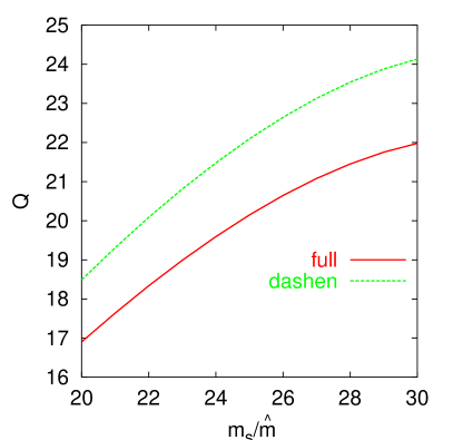
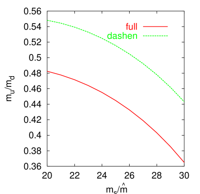
Figure 3: (a) $Q$ (b) $m_{u}/m_{d}$ as a function of $m_{s}/\hat{m}$ but other input fixed as in the main fit.

The position of the previous mentioned ellipsis can be described as the ratio of $SU(3)$ breaking effects versus $SU(2)$ isospin breaking using

$$R\equiv\frac{m_{s}-\hat{m}}{m_{d}-m_{u}}\,.$$ (58)

The standard value [40] used $\rho$-$\omega$ mixing and combinations of the baryon masses to obtain $R=43.5\pm 2.2$. Both of these inputs are now known to have rather large corrections of ${\cal O}(m_{q})$. $\rho$-$\omega$ mixing is treated in [46] and results for the baryon masses with earlier references can be found in [47]. We obtain for this quantity

$$R\approx 31~{}\mbox{[Eq. (\ref{BPdashen})]}\,;\quad 37~{}\mbox{[Eq. (\ref{dashen})]}\,.\\$$ (59)

One of the main results from Table 1 is

$$\frac{m_{u}}{m_{d}}=0.46\pm 0.09\,.$$ (60)

In the previous estimate the error is increased w.r.t. the one of the fit in order to include two other sources of errors, about 0.02 from the error on the electromagnetic correction due to $m_{K^{\pm}}^{2}-m_{K^{0}}^{2}$ and another 0.02 from the rather large change that happened with the scale variation at $\mu=1$ GeV. The other new result we obtain is the strong mass difference

$$\delta m_{\pi}=\left(m_{\pi^{\pm}}-m_{\pi^{0}}\right)_{\mbox{\tiny QCD}}=0.32\pm 0.20~{}\mbox{MeV}\,.$$ (61)

The change with the result quoted in [1] has two sources, about 0.04 MeV from the inclusion of the mass-corrections in the Kaon electromagnetic mass difference and the remainder comes from the ${\cal O}(p^{6})$ effects.

A possibly more serious variation with input is due to the assumptions on $L_{4}^{r}$ and $L_{6}^{r}$. Our tests of large $N_{c}$ as described in Sect. 5.2 are mainly in quantities dominated by vector exchange. We have therefore checked what happens when we vary the input value of $L_{4}^{r}$ and $L_{6}^{r}$ over a fairly wide range. The resulting values for $m_{u}/m_{d}$ are plotted in Fig. 4.

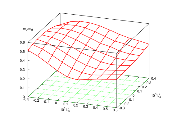
Figure 4: The ratio $m_{u}/m_{d}$ versus the inputs for $L_{4}^{r},L_{6}^{r}$ the rest of parameters correspond to those of our main fit.

It should be kept in mind that not all of the points shown have good fits to all inputs and most of the points actually fall in the range of Eq. (60). It is a rather clear conclusion that the value $m_{u}/m_{d}=0$ is far away from the numbers we have obtained. Unfortunately this means that the solution to the strong CP problem needs to be found elsewhere.

10 Summary

In this paper we have explained how isospin breaking effects can be incorporated at next-to-next-to-leading order in CHPT. The expectation that isospin breaking would not significantly alter our previous results has been confirmed and the results presented here are a first step in understanding how isospin breaking effects can be added consistently.

We have reanalyzed the main fit at ${\cal O}(p^{6})$ of the CHPT LEC’s in the presence of isospin breaking. The determination of the $L_{i}^{r}$ is only marginally changed compared to the isospin symmetric analysis. As by product we obtain control on the quantity $m_{u}/m_{d}$ at next-to-next-to-leading order in terms of meson masses. This constitutes one of our main new results.

Furthermore using the preliminary new experimental results on $K_{\ell 4}$ we can obtain one of the Zweig Rule suppressed LEC, namely $L_{4}^{r}$. It follows approximately a linear relation together with $L_{6}^{r}$.

We also revised the value of the isospin breaking quantities $Q$ and $R$ discussing the electromagnetic effects. In view of the low value of Eq. (57) a reanalysis of the $\eta\to 3\pi$ decay at the same order in the quark mass expansion as was done here seems necessary.

Acknowledgements
G.A and P.T. were supported by TMR, EC–Contract No. ERBFMRX–CT980169 (EURODAPHNE).

References

- [1] J. Gasser and H. Leutwyler, Nucl. Phys. B250 (1985) 465.
- [2] G. Amoros, J. Bijnens and P. Talavera, Nucl. Phys. B568 (2000) 319 [hep-ph/9907264].
- [3] G. Amoros, J. Bijnens and P. Talavera, Phys. Lett. B480 (2000) 71 [hep-ph/9912398]; Nucl. Phys. B585 (2000) 293 [hep-ph/0003258].
- [4] H. Leutwyler and M. Roos, Z. Phys. C25 (1984) 91.
- [5] P. Truol et al. [E865 Collaboration], hep-ex/0012012.
- [6] G. Ecker, “Strong interactions of light flavours,” hep-ph/0011026; A. Pich, “Effective field theory,” hep-ph/9806303.
- [7] G. Ecker, G. Muller, H. Neufeld and A. Pich, Phys. Lett. B477 (2000) 88 [hep-ph/9912264].
- [8] J. Bijnens, G. Colangelo, G. Ecker, J. Gasser and M. E. Sainio, Nucl. Phys. B508 (1997) 263 [hep-ph/9707291].
- [9] R. Urech, Nucl. Phys. B433 (1995) 234 [hep-ph/9405341].
- [10] M. Knecht, H. Neufeld, H. Rupertsberger and P. Talavera, Eur. Phys. J. C12 (2000) 469 [hep-ph/9909284] and work in progress.
- [11] R. Dashen, Phys. Rev. 183 (1969) 1245.
- [12] H. Neufeld and H. Rupertsberger, Z. Phys. C68 (1995) 91; Z. Phys. C71 (1996) 131 [hep-ph/9506448].
- [13] J. Bijnens, Phys. Lett. B306 (1993) 343 [hep-ph/9302217].
- [14] J. F. Donoghue, B. R. Holstein and D. Wyler, Phys. Rev. D47 (1993) 2089.
- [15] A. Duncan, E. Eichten and H. Thacker, Phys. Rev. Lett. 76 (1996) 3894 [hep-lat/9602005]; Nucl. Phys. Proc. Suppl. 53 (1997) 295 [hep-lat/9609015].
- [16] J. Bijnens and J. Prades, Nucl. Phys. B490 (1997) 239 [hep-ph/9610360].
- [17] R. Baur and R. Urech, Phys. Rev. D53 (1996) 6552 [hep-ph/9508393].
- [18] B. R. Holstein, Phys. Lett. B244 (1990) 83.
- [19] M. Finkemeier, Phys. Lett. B387 (1996) 391 [hep-ph/9505434].
- [20] L. Rosselet et al., Phys. Rev. D15 (1977) 574.
- [21] G. Ecker, J. Gasser, A. Pich and E. de Rafael, Nucl. Phys. B321 (1989) 311; G. Ecker et. al., Phys. Lett. B223 (1989) 425.
- [22] D. Espriu, E. de Rafael and J. Taron, Nucl. Phys. B345 (1990) 22; J. Bijnens, C. Bruno and E. de Rafael, Nucl. Phys. B390 (1993) 501 [hep-ph/9206236]; J. Bijnens, Phys. Rept. 265 (1996) 369 [hep-ph/9502335]; S. Peris, M. Perrottet and E. de Rafael, JHEP 9805 (1998) 011 [hep-ph/9805442].
- [23] E. Golowich and J. Kambor, Nucl. Phys. B447 (1995) 373 [hep-ph/9501318]; Phys. Rev. D58 (1998) 036004 [hep-ph/9710214]; S. Durr and J. Kambor, Phys. Rev. D 61 (2000) 114025 [hep-ph/9907539].
- [24] J. Bijnens, G. Colangelo and P. Talavera, JHEP 9805 (1998) 014 [hep-ph/9805389].
- [25] C. A. Dominguez and E. de Rafael, Annals Phys. 174 (1987) 372; J. Bijnens, J. Prades and E. de Rafael, Phys. Lett. B348 (1995) 226 [hep-ph/9411285]; S. Narison, Nucl. Phys. Proc. Suppl. 86 (2000) 242 [hep-ph/9911454].
- [26] K. G. Chetyrkin, C. A. Dominguez, D. Pirjol and K. Schilcher, Phys. Rev. D51 (1995) 5090 [hep-ph/9409371]; M. Jamin and M. Munz, Z. Phys. C66 (1995) 633 [hep-ph/9409335]; K. G. Chetyrkin, D. Pirjol and K. Schilcher, Phys. Lett. B404 (1997) 337 [hep-ph/9612394]; P. Colangelo, F. De Fazio, G. Nardulli and N. Paver, Phys. Lett. B408 (1997) 340 [hep-ph/9704249]; K. Maltman, Phys. Lett. B462 (1999) 195 [hep-ph/9904370]; A. Pich and J. Prades, JHEP9910 (1999) 004 [hep-ph/9909244]; J. Kambor and K. Maltman, Phys. Rev. D 62 (2000) 093023 [hep-ph/0005156].
- [27] B. Moussallam, Eur. Phys. J. C14 (2000) 111 [hep-ph/9909292].
- [28] S. Descotes and J. Stern, Phys. Lett. B488 (2000) 274 [hep-ph/0007082]; S. Descotes, hep-ph/0012221.
- [29] S. Pislak, in talk given at Laboratori Nazionali di Frascati , Rome, Italy, June 22, 2000, unpublished.
- [30] G. Amoros and J. Bijnens, J. Phys. G25 (1999) 1607 [hep-ph/9902463].
- [31] J. Bijnens, Nucl. Phys. B337 (1990) 635; C. Riggenbach et al., Phys. Rev. D 43 (1991) 127.
- [32] J. Bijnens, G. Colangelo and J. Gasser, Nucl. Phys. B427 (1994) 427 [hep-ph/9403390].
- [33] G. Makoff et al., Phys. Rev. Lett. 70 (1993) 1591; Erratum-ibid. 75 (1995) 2069.
- [34] J. Heitger, R. Sommer and H. Wittig [ALPHA Collaboration], Nucl. Phys. B588 (2000) 377 [hep-lat/0006026].
- [35] H. Leutwyler and A. Smilga, Phys. Rev. D46 (1992) 5607.
- [36] J. Stern, [hep-ph/9801282] and in talk given at Workshop on Chiral Dynamics: Theory and Experiment (ChPT 97), Mainz, Germany, 1-5 Sep 1997. [hep-ph/9712438].
- [37] M. A. Shifman, A. I. Vainshtein and V. I. Zakharov, Nucl. Phys. B147 (1979) 519.
- [38] S. Narison, Phys. Lett. B104 (1981) 485; E. Bagan, A. Bramon, S. Narison and N. Paver, Phys. Lett. B135 (1984) 463.
- [39] P. Pascual and R. Tarrach, Phys. Lett. B116 (1982) 443; L. J. Reinders, H. R. Rubinstein and S. Yazaki, Phys. Lett. B120 (1983) 209. Erratum-ibid. B122 (1983) 487.
- [40] J. Gasser and H. Leutwyler, Phys. Rept. 87 (1982) 77.
- [41] D. E. Groom et al., Eur. Phys. J. C15 (2000) 1.
- [42] D. B. Kaplan and A. V. Manohar, Phys. Rev. Lett. 56 (1986) 2004.
- [43] H. Leutwyler, “Non-lattice determinations of the light quark masses,” hep-ph/0011049; Phys. Lett. B378 (1996) 313 [hep-ph/9602366].
- [44] J. Gasser and H. Leutwyler, Nucl. Phys. B250 (1985) 539.
- [45] J. Kambor, C. Wiesendanger and D. Wyler, Nucl. Phys. B465 (1996) 215 [hep-ph/9509374]; A. V. Anisovich and H. Leutwyler, Phys. Lett. B375 (1996) 335 [hep-ph/9601237].
- [46] J. Bijnens, P. Gosdzinsky and P. Talavera, Nucl. Phys. B501 (1997) 495 [hep-ph/9704212].
- [47] B. Borasoy and U. Meissner, Annals Phys. 254 (1997) 192 [hep-ph/9607432].