Sphalerons in Two Higgs Doublet Theories

Abstract

We undertake a comprehensive investigation of the properties of the sphaleron in electroweak theories with two Higgs doublets. We do this in as model-independent a way as possible: by exploring the physical parameter space described by the masses and mixing angles of the Higgs particles. If there is a large split in the masses of the neutral Higgs particles, there can be several sphaleron solutions, distinguished by their properties under parity and the behaviour of the Higgs field at the origin. In general, these solutions appear in parity conjugate pairs and are not spherically symmetric, although the departure from spherical symmetry is small. Including CP violation in the Higgs potential can change the energy of the sphaleron by up to 14 percent for a given set of Higgs masses, with significant implications for the baryogenesis bound on the mass of the lightest Higgs.

PACS numbers: 11.15.-q, 11.27.+d, 11.30.-j SUSX-TH-00-003

1 Introduction

One of the major unsolved problems in particle cosmology is to account for the baryon asymmetry of the Universe. This asymmetry is usually expressed in terms of the parameter $\eta$, defined as the ratio between the baryon number density $n_{B}$ and the entropy density $s$: $\eta=n_{B}/s\sim 10^{-10}$. Sakharov [1] laid down the framework for any explanation: the theory of baryogenesis must contain baryon number ($B$) violation; charge conjugation ($C$) violation; combined charge conjugation and parity ($CP$) violation; and a departure from thermal equilibrium. The Standard Model is naturally $C$ and $P$ violating, and violates $CP$ through the couplings of fermionic charged currents to the $W^{\pm}$ (the CKM matrix). It was also known to violate the combination $B+L$ (where $L$ is lepton number) non-perturbatively [2], and the realisation that this rate is large at high temperature, and that the Standard Model could depart from equilibrium at a first order phase transition [3] led to considerable optimism that the origin of the baryon asymmetry could be found in known physics.

However, the Standard Model does not have a first order phase transition for Higgs masses above about 75 GeV [4, 5], and in any case is not thought to have enough $CP$ violation. Current attention is focused on the Minimal Supersymmetric Standard Model (MSSM), where there are many sources of $CP$ violation over and above the CKM matrix [6, 7, 8], and the phase transition can be first order for Higgs masses up to 120 GeV, provided the right-handed stop is very light and the left-handed stop very massive [9, 10, 11].

The currently accepted picture for the way these elements fit together was developed by Cohen, Kaplan, and Nelson [12] (see also [13, 14, 15] for reviews). A first order transition proceeds by nucleation of bubbles of the new, stable, phase. The bubbles grow and merge until the new phase has taken over. The effect of $CP$ violation in the theory is to make the fermion reflection coefficients off the wall chirally asymmetric, which results in a chiral asymmetry building up in front of the advancing wall in the fermion species which couple most strongly to the wall and have the largest $CP$ violating couplings. This chiral asymmetry is turned into a baryon asymmetry by the action of symmetric-phase sphalerons.

As the wall sweeps by, the rate of baryon number violation by sphalerons drops as the sphaleron mass increases sharply. The formation of a sphaleron is a thermal activation process and the rate can be estimated to go as $\Gamma_{s}\simeq\exp(-E_{s}(T)/T)$, where $E_{s}(T)$ is the energy of the sphaleron at temperature $T$. This rate must not be so large that the baryon asymmetry is removed behind the bubble wall by sphaleron processes in thermal equilibrium, and this condition can be translated into a lower bound on the sphaleron mass [16, 17, 18]

$$E_{s}(T_{c})/T_{c}\mathrel{\mathchoice{\lower 0.5pt\vbox{\halign{$\math\displaystyle\hfil#\hfil$\cr\scriptstyle>\crcr{\scriptstyle\sim}\crcr}}}{\lower 0.5pt\vbox{\halign{$\math\textstyle\hfil#\hfil$\cr\scriptstyle>\crcr{\scriptstyle\sim}\crcr}}}{\lower 0.5pt\vbox{\halign{$\math\scriptstyle\hfil#\hfil$\cr\scriptstyle>\crcr{\scriptstyle\sim}\crcr}}}{\lower 0.5pt\vbox{\halign{$\math\scriptscriptstyle\hfil#\hfil$\cr\scriptstyle>\crcr{\scriptstyle\sim}\crcr}}}}45.$$ (1)

Thus it is clear that any theory of baryogenesis requires a careful calculation of the sphaleron mass. For example, it turns out that condition (1) is not satisfied for any value of Higgs mass in the Standard Model [4].

It has been known for a long time that spherically symmetric solutions exist in SU(2) gauge theory with a single fundamental Higgs [19, 20, 21], which is the bosonic sector of the Standard Model at zero Weinberg angle. However, it was Klinkhamer and Manton [22] who realised that they were unstable, with a single unstable mode, and that the formation and decay of a sphaleron results in a simultaneous change of both $B$ and $L$ number by $N_{f}$ (the number of fermion families). They calculated numerically both the mass and the Chern-Simons number, finding the mass to be 3.7 (4.2) $M_{W}/\alpha_{W}$ at a Higgs mass of 72 (227) GeV, where $\alpha_{W}=g_{W}^{2}/4\pi$ and $M_{W}$ is the mass of the $W^{\pm}$ particle; and the Chern-Simons number to be exactly 1/2.

At $M_{h}\mathrel{\mathchoice{\lower 0.5pt\vbox{\halign{$\math\displaystyle\hfil#\hfil$\cr\scriptstyle>\crcr{\scriptstyle\sim}\crcr}}}{\lower 0.5pt\vbox{\halign{$\math\textstyle\hfil#\hfil$\cr\scriptstyle>\crcr{\scriptstyle\sim}\crcr}}}{\lower 0.5pt\vbox{\halign{$\math\scriptstyle\hfil#\hfil$\cr\scriptstyle>\crcr{\scriptstyle\sim}\crcr}}}{\lower 0.5pt\vbox{\halign{$\math\scriptscriptstyle\hfil#\hfil$\cr\scriptstyle>\crcr{\scriptstyle\sim}\crcr}}}}12M_{W}$ new solutions appear [23, 24], which have different boundary conditions at the origin: the Higgs field does not vanish. These spontaneously violate parity and occur in $P$ conjugate pairs with slightly lower energy than the original sphaleron, which correspondingly develops a second negative eigenvalue. These are termed deformed sphalerons or bisphalerons.

Several authors have considered models with two Higgs doublets. Kastening, Peccei, and Zhang (KPZ) [25] studied models with $CP$ violation, but did not use the most general spherically symmetric ansatz, limiting themselves to a parity conserving form. Bachas, Tinyakov, and Tomaras (BTT) [26] on the other hand, considered a two-doublet theory with no explicit $CP$ violation, used a $C$ conserving ansatz, chose the masses of the pseudoscalar ($M_{A}$) and the charged Higgs ($M_{H^{\pm}}$) to be zero, and chose the mixing between the two scalar Higgses to be zero. They found new $P$ violating solutions, specific to multi-doublet models, at $M_{H}\mathrel{\mathchoice{\lower 0.5pt\vbox{\halign{$\math\displaystyle\hfil#\hfil$\cr\scriptstyle>\crcr{\scriptstyle\sim}\crcr}}}{\lower 0.5pt\vbox{\halign{$\math\textstyle\hfil#\hfil$\cr\scriptstyle>\crcr{\scriptstyle\sim}\crcr}}}{\lower 0.5pt\vbox{\halign{$\math\scriptstyle\hfil#\hfil$\cr\scriptstyle>\crcr{\scriptstyle\sim}\crcr}}}{\lower 0.5pt\vbox{\halign{$\math\scriptscriptstyle\hfil#\hfil$\cr\scriptstyle>\crcr{\scriptstyle\sim}\crcr}}}}5M_{W}$, where $M_{H}$ is the mass of the second $CP$ even Higgs. They did not calculate the Chern-Simons number, but we show that these solutions appear in $P$ conjugate pairs and are in fact sphalerons, in that they have Chern-Simons number near 1/2, and one unstable mode. In view of the difference in behaviour of the two Higgs fields as the origin is approached, we call them relative winding (RW) sphalerons. More recently, Kleihaus [27] looked at the bisphalerons in a restricted two-doublet Higgs model.

Sphalerons in the MSSM have were studied by Moreno, Oaknin, and Quiros (MOQ) [28], who included one-loop corrections, both quantum and thermal. However, they again did not allow for $P$ violating bisphalerons or RW sphalerons, and did not consider the effect of $CP$ violation either, which can appear in the guise of complex values of the soft SUSY breaking terms in the potential.

All of the above work was carried out at zero Weinberg angle with a spherically symmetric ansatz: there have been several studies of sphalerons in the Standard Model in the full SU(2)$\times$U(1) theory [29, 30, 31], where one is forced to adopt the more complicated axially symmetric ansatz: Ref. [29] used the axially symmetric ansatz in a numerical computaton, [30] expanded in powers of $g^{\prime}/g$ using a partial wave decomposition, and [31] estimated the energy by constructing a non-contractible loop in field configuration space which was sensitive to $\theta_{W}$. The upshot of this work is that working at the physical value of the Weinberg angle changes the energy of the sphaleron by about 10%. It is interesting to note that the SU(2)$\times$U(1) theory also contains charged sphaleron solutions [32].

Here we report on work on sphalerons in the two-doublet Higgs model (2DHM) in which we study the properties of sphalerons in as general a set of realistic models as possible, although we do use the zero Weinberg angle approximation and a spherically symmetric ansatz. We try to express parameter space in terms of physical quantities: Higgs masses and mixing angles, which helps us avoid regions of parameter space which have already been ruled out by LEP, or where the vacuum is unstable. It also means one can take into account ultraviolet radiative corrections by using the 1-loop corrected values for the masses and mixing angles.

We are interested in the energy, the Chern-Simons number, the symmetry properties, and the eigenvalues of the normal modes of the various sphaleron solutions in the theory, as functions of the physical parameters. From the point of view of the computation of the rate of baryon number violation, the mass is certainly the most important quantity, followed by the number and magnitude of negative eigenvalues of the fluctuation operator in the sphaleron background: the largest contribution to the baryon number violation rate comes from the sphaleron with lowest energy and hence only one negative eigenvalue. The Chern-Simons number and the symmetry properties under $C$, $P$, and spatial rotations, are also interesting as they help classify the solutions.

We firstly check our results against the existing literature, principally Yaffe [24] and BTT [26], and then reexamine the sphaleron in a more realistic part of parameter space, where $M_{A}$ and $M_{H^{\pm}}$ are above their experimental bounds. We find that in large regions of parameter space, particularly when one of the neutral Higgses is heavy (above about 6 $M_{W}$), the RW sphaleron is the lowest energy sphaleron. When there is $CP$ violation in the Higgs sector, the would-be pseudoscalar Higgs can play the role of the heavy Higgs, and the other two Higgses can remain relatively light. The fractional energy difference between the RW and the ordinary (Klinkhamer-Manton) sphaleron is small, about 1% in the parameter ranges we explored.

We encounter a problem with $P$ violating sphalerons when either $M_{A}-M_{H^{\pm}}$, or the amount of $CP$ violation is non-zero: there is a departure from spherical symmetry in the energy density, signalling an inconsistency in the ansatz for the field profiles. However, the energy density in the non-spherically symmetric terms is small, at most about 0.2% of the dominant spherically symmetric terms, so it is a good approximation to ignore them.

We also looked at the sphaleron in the restricted parameter space afforded by the (tree level) MSSM, confirming the results of [28] that the sphaleron energy depends mainly on the mass of the lightest Higgs and on $\tan\beta$, and finding no RW or bisphaleron solutions.

Finally, we amplify the point made in [33] that introducing $CP$ violation makes a significant difference to the sphaleron mass, and may significantly change bounds on the Higgs mass from electroweak baryogenesis.

We do not explicitly compute quantum or thermal corrections [18, 34, 35, 36, 37, 38, 39] as they are model-dependent. However, if particle masses are expressed in units of $M_{W}$, a reasonable approximation to the 1-loop sphaleron mass (in units of $M_{W}/\alpha_{W}$) can be obtained by interpreting the masses and mixing angles as loop-corrected quantities evaluated at an energy scale $M_{W}$ [39]. This approximation justifiably ignores small corrections due to radiatively induced operators of dimension higher than 4, but does not take into account the cubic term in the effective potential. This means our calculations are less accurate near the phase transition. However, as the error is in the Higgs potential, which generally contributes less than 10% to the energy, the resulting uncertainty is not large.

The plan of the paper is as follows. In Section 2 we describe the bosonic sector of the two Higgs doublet SU(2) electroweak theory. We discuss the various parametrizations of the scalar potential, and provide translation tables in Appendix A. We show how we use physical masses and mixing angles as independent parameters of the theory. Although in this approach the stability of the vacuum is automatic, as one chooses the masses of the physical particles to be real, there are still the problems of boundedness and global minimisation to be overcome. We solve the boundedness problem straight forwardly, but with two Higgs doublets, finding the global minimum of the potential is non-trivial, and we are forced to use numerical methods.

In Section 3 we discuss the sphaleron solutions and their symmetry properties. In Section 4 we descibe the numerical method we use to find the solutions: although the Newton method has been used before [24, 26] there are some difficulties associated with the boundary conditions that were not highlighted by previous authors. In Section 5 we present our results. Section 6 contains discussions and conclusions.

Throughout this paper we use $\hbar=c=k_{B}=1$, a metric with signature $(+,-,-,-)$, and $M_{W}=80.4$ GeV.

2 Two Higgs doublet electroweak theory

We shall be working with an SU(2) theory with two Higgs doublets $\phi_{\alpha}$, with subscript $\alpha=1,2$. Although we should strictly work with the full SU(2)$\times$U(1) theory, neglecting the U(1) coupling is a reasonable approximation to make when studying the sphaleron.

The relevant Lagrangian is

$${\cal L}=-\frac{1}{4}F^{a}_{\mu\nu}F^{a\mu\nu}+(D_{\mu}\phi_{\alpha})^{\dagger}(D^{\mu}\phi_{\alpha})-V(\phi_{1},\phi_{2}).$$ (2)

Here, the covariant derivative $D_{\mu}\phi_{\alpha}=\partial_{\mu}\phi_{\alpha}+gW^{a}_{\mu}t^{a}\phi_{\alpha}$ with antihermitian generators $t^{a}=\sigma^{a}/2i$.

This Lagrangian may have discrete symmetries, including parity, charge conjugation invariance, and $CP$ [40]. These transformations are realised on the Higgs fields by

$$P: \phi_{\alpha}(t,x^{j})\to\phi_{\alpha}(t,-x^{j}),$$ (3)

$$C: \phi_{\alpha}(t,x^{j})\to{-i}\sigma_{2}e^{-i2\theta_{\alpha}}\phi_{\alpha}^{\ast}(t,x^{j}),$$ (4)

$$CP: \phi_{\alpha}(t,x^{j})\to{-i}\sigma_{2}e^{-i2\theta_{\alpha}}\phi_{\alpha}^{\ast}(t,-x^{j}),$$ (5)

where $\theta_{\alpha}$ are phase factors that can only be determined by reference to the complete theory. The transformations on the gauge fields are

$$P: W_{\mu}(t,x^{j})\to W^{\mu}(t,-x^{j}),$$ (6)

$$C: W_{\mu}(t,x^{j})\to({-i}\sigma_{2})W_{\mu}^{\ast}(t,x^{j})({-i}\sigma_{2})^{\dagger},$$ (7)

$$CP: W_{\mu}(t,x^{j})\to({-i}\sigma_{2})W^{\mu\ast}(t,-x^{j})({-i}\sigma_{2})^{\dagger}.$$ (8)

With these transformations the only place a departure from $C$, $P$, or $CP$ invariance can occur in Lagrangian (2) is in the Higgs potential term $V(\phi_{1},\phi_{2})$.

2.1 The Higgs potential

The most general two Higgs doublets potential has 14 real parameters, assuming that the energy density at the minimum is zero. We shall consider one with a discreet symmetry imposed on dimension four terms, $\phi_{1}\rightarrow\phi_{1}$, $\phi_{2}\rightarrow-\phi_{2}$, which suppresses flavour changing neutral currents [41], and results in a potential with 10 real parameters. One of these parameters may be removed by a phase redefinition of the fields we detail in Appendix A, and the potential may be written

$$V(\phi_{1},\phi_{2}) = (\lambda_{1}+\lambda_{3})\left(\phi_{1}^{\dagger}\phi_{1}-\frac{\upsilon_{1}^{2}}{2}\right)^{2}+(\lambda_{2}+\lambda_{3})\left(\phi_{2}^{\dagger}\phi_{2}-\frac{\upsilon_{2}^{2}}{2}\right)^{2}$$ (9)

$$+2\lambda_{3}\left(\phi_{1}^{\dagger}\phi_{1}-\frac{\upsilon_{1}^{2}}{2}\right)\left(\phi_{2}^{\dagger}\phi_{2}-\frac{\upsilon_{2}^{2}}{2}\right)$$

$$+\lambda_{4}\left[\phi_{1}^{\dagger}\phi_{1}\phi_{2}^{\dagger}\phi_{2}-\mathrm{Re}^{2}(\phi_{1}^{\dagger}\phi_{2})-\mathrm{Im}^{2}(\phi_{1}^{\dagger}\phi_{2})\right]$$

$$+(\lambda_{+}+\chi_{1})\left(\mathrm{Re}(\phi_{1}^{\dagger}\phi_{2})-\frac{\upsilon_{1}\upsilon_{2}}{2}\right)^{2}+(\lambda_{+}-\chi_{1})\mathrm{Im}^{2}(\phi_{1}^{\dagger}\phi_{2})$$

$$+2\chi_{2}\left(\mathrm{Re}(\phi_{1}^{\dagger}\phi_{2})-\frac{\upsilon_{1}\upsilon_{2}}{2}\right)\mathrm{Im}(\phi_{1}^{\dagger}\phi_{2}).$$

This form of the potential is convenient as the vacuum configuration, which we take as the zero of the potential is entirely real:

$$\phi^{vac}_{\alpha}=\frac{\upsilon_{\alpha}}{\sqrt{2}}\left[\begin{array}[]{c}0\\ 1\end{array}\right].$$ (10)

This form also makes clear what are the sources of $CP$ violation in the theory. Ignoring couplings to other fields, it can be seen that when $\chi_{2}=0$ there is a discrete symmetry

$$\phi_{\alpha}\rightarrow{-i}\sigma_{2}\phi_{\alpha}^{\ast},$$ (11)

which sends $\mathrm{Im}(\phi_{1}^{\dagger}\phi_{2})\to-\mathrm{Im}(\phi_{1}^{\dagger}\phi_{2})$. This can be identified as charge conjugation invariance. Thus $\chi_{2}$ is a $C$ breaking parameter. In the presence of fermions, $C$ and $P$ are not separately conserved, and we generally refer to the field properties according to their behavior under $CP$, and to $\chi_{2}$ as a $CP$ violating parameter, giving rise to a mixing between the $CP$ odd and $CP$ even neutral Higgses. When one includes the other fields of the full theory one can find further sources of $CP$ violation, such as the phases in the CKM matrices of the quarks and, if neutrinos are massive, leptons.

In Appendix A we write down how the nine parameters of Eq. 9 relate to the parameters of the two more usual forms of this potential.

It is useful to determine as many as possible of the nine parameters in the potential from physical ones. The physical parameters at hand are the four masses of the Higgs particles, the three mixing angles of the neutral Higgses, and the vacuum expectation value ($\upsilon$) of the Higgs (which is determined from $M_{W}$, and the SU(2) gauge coupling $g$). This leaves one undetermined parameter which may be chosen in various ways.

In the absence of $CP$ violation, we automatically have $\chi_{2}=0$, and our input parameters are; $\upsilon$, $M_{h}$ and $M_{H}$ (the masses of the $CP$ even scalars), $M_{A}$ (the mass of the $CP$ odd scalar), $M_{H^{\pm}}$ (the mass of the charged scalar), $\phi$ (the mixing angle between the $CP$ even scalars), $\tan\beta$ and $\lambda_{3}$, (the only parameter we choose by hand). This gives non-zero values for the other eight of our nine parameters.

In the presence of $CP$ violation our input parameters again include $\upsilon$, $M_{h}$, $M_{H}$, $M_{A}$, $M_{H^{\pm}}$, $\phi$, and $\lambda_{3}$. However, now we also have $\theta_{CP}$ (the mixing angle between the $CP$ even and the $CP$ odd neutral Higgs sector which is entirely responsible for the $\chi_{2}$ term), and the third mixing angle $\psi$. For a non-zero $\theta_{CP}$, $\tan\beta$ is determined by the masses and mixings, and although we still denote the three neutral Higgs masses as $M_{h}$, $M_{H}$, and $M_{A}$ we stress that they are not respectively $CP$ even, $CP$ even, and $CP$ odd, but have some combination of these properties depending on the values of $\theta_{CP}$ and $\phi$.

The conversion between the parameters of Eq.  9 and these masses and mixings is carried out in the charged sector through

$$\lambda_{4}=\frac{2M_{H^{\pm}}^{2}}{\upsilon^{2}},$$ (12)

and in the neutral sector by writing

$$\upsilon^{2}X\equiv D^{-1}(\psi,\theta_{CP},\phi)~{}M_{P}(M_{h},M_{H},M_{A})~{}D(\psi,\theta_{CP},\phi),$$ (13)

where $M_{P}$ is a diagonal mass matrix given by

$$M_{P}\equiv{\rm Diag}\left[M_{H}^{2},M_{h}^{2},M_{A}^{2}\right],$$ (14)

and $D$ is the orthogonal matrix which diagonalises $X$. Defining rotation matrices in the usual way,

$$R_{z}(\alpha)=\left[\begin{array}[]{ccc}\cos\alpha&\sin\alpha&0\\ -\sin\alpha&\cos\alpha&0\\ 0&0&1\end{array}\right],~{}~{}~{}~{}~{}~{}R_{y}(\alpha)=\left[\begin{array}[]{ccc}\cos\alpha&0&-\sin\alpha\\ 0&1&0\\ \sin\alpha&0&\cos\alpha\end{array}\right],$$ (15)

we can arrange for the mixing angles $\psi,\theta_{CP},\phi$ to be the usual Euler angles, through

$$D(\psi,\theta_{CP},\phi)\equiv R_{z}(\psi)R_{y}(\theta)R_{z}(\phi).$$ (16)

The $X(\psi,\theta_{CP},\phi,M_{h},M_{H},M_{A})$ of Eq. 13 can be obtained as a function of the parameters of Eq.  9, by expanding about the vacuum state Eq.  10, to give

$$X(1,1) = \frac{1}{2}\left[4(\lambda_{1}+\lambda_{3})\cos^{2}\beta+(\lambda_{+}+\chi_{1})\sin^{2}\beta\right],$$ (17)

$$X(1,2) = X(2,1)=\frac{1}{2}(4\lambda_{3}+\lambda_{+}+\chi_{1})\cos\beta\sin\beta,$$ (18)

$$X(1,3) = X(3,1)=\frac{1}{2}\chi_{2}\sin\beta,$$ (19)

$$X(2,2) = \frac{1}{2}\left[4(\lambda_{2}+\lambda_{3})\sin^{2}\beta+(\lambda_{+}+\chi_{1})\cos^{2}\beta\right],$$ (20)

$$X(2,3) = X(3,2)=\frac{1}{2}\chi_{2}\cos\beta,$$ (21)

$$X(3,3) = \frac{1}{2}(\lambda_{+}-\chi_{1}).$$ (22)

Inverting Eqs.  17-22 gives

$$\chi_{2} = 2\sqrt{X(1,3)^{2}+X(2,3)^{2}},$$ (23)

$$\beta = \arctan\left[{X(1,3)}/{X(2,3)}\right],$$ (24)

$$\lambda_{1} = \left[X(1,1)\cos\beta-X(1,2)\sin\beta-2\lambda_{3}\cos 2\beta\cos\beta\right]\frac{1}{2\cos^{3}\beta},$$ (25)

$$\lambda_{2} = \left[X(2,2)\sin\beta-X(1,2)\cos\beta+2\lambda_{3}\cos 2\beta\sin\beta\right]\frac{1}{2\sin^{3}\beta},$$ (26)

$$\lambda_{+} = -2\lambda_{3}+X(1,2)\frac{1}{\sin\beta\cos\beta}+X(3,3),$$ (27)

$$\chi_{1} = -2\lambda_{3}+X(1,2)\frac{1}{\sin\beta\cos\beta}-X(3,3),$$ (28)

where the $X$ above are the $X(\psi,\theta_{CP},\phi,M_{h},M_{H},M_{A})$ as given by Eq.  13. And we have chosen $-\pi<2\beta<\pi$ from which, depending on the sign of $X(1,2)$ and $X(1,3)$, we can set the sign of $\chi_{2}$. Although it is unconventional to allow $\beta$ to take negative values, it is a natural consequence of allowing the mixing angles to vary over their full range.

2.2 Boundedness and stability of the Higgs potential

Before proceeding, we re-examine the conditions on our potential which derive from its boundedness and the stability of the vacuum state. For boundedness we need consider only the quartic terms of Eq.  9 to find the large field behaviour of the potential. We write our doublets as

$$\phi_{\alpha}=\left|\sqrt{\rm{Q}_{\alpha}}\right|\left[\begin{array}[]{c}\cos\rho_{\alpha}e^{i\kappa_{\alpha}}\\ \sin\rho_{\alpha}e^{i\omega\alpha}\end{array}\right],$$ (29)

this will allow us to express the potential in terms of independent quantities. The quartic terms of Eq. 9 can then be written as

$$V=aQ_{1}^{2}+bQ_{2}^{2}+c(\eta_{1},\eta_{2})Q_{1}Q_{2},$$ (30)

where

$$\eta_{1} = \cos\rho_{1}\cos\rho_{2}\cos(\kappa_{2}-\kappa_{1})+\sin\rho_{1}\sin\rho_{2}\cos(\omega_{2}-\omega_{1}),$$ (31)

$$\eta_{2} = \cos\rho_{1}\cos\rho_{2}\sin(\kappa_{2}-\kappa_{1})+\sin\rho_{1}\sin\rho_{2}\sin(\omega_{2}-\omega_{1}),$$ (32)

and

$$a=\lambda_{1}+\lambda_{3},$$ (33)

$$b=\lambda_{2}+\lambda_{3},$$ (34)

$$c(\eta_{1},\eta_{2})=2\lambda_{3}+\lambda_{4}+(\lambda_{+}-\lambda_{4}+\chi_{1})\eta_{1}^{2}+(\lambda_{+}-\lambda_{4}-\chi_{1})\eta_{2}^{2}+2\chi_{2}\eta_{1}\eta_{2}.$$ (35)

The variables $Q_{1}$, $Q_{2}$, $\eta_{1}$, and $\eta_{2}$ are then independent. Furthermore, $Q_{1}$ and $Q_{2}$ are by definition non-negative, and $\eta_{1}$ and $\eta_{2}$ are constrained to lie in the unit disc

$$0\leq\eta_{1}^{2}+\eta_{2}^{2}\leq 1.$$ (36)

The potential can now be viewed as a quadratic form in $Q_{1}$, $Q_{2}$, in which case the form must be positive for all values of $\eta_{1}$, $\eta_{2}$ in the unit disc. If $c_{min}(\eta_{1},\eta_{2})$ is the minimum value of $c(\eta_{1},\eta_{2})$ for all $\eta_{1}$ and $\eta_{2}$, the condition for the form to be positive and the potential bounded are

$$a+b \geq 0,$$ (37)

$$ab-\frac{c^{2}_{min}}{4} \geq 0.$$ (38)

On substituting the values of $a$, $b$, and $c_{min}$ into Eqs. 37 and 38 we obtain

$$\lambda_{1}+\lambda_{2}+2\lambda_{3} \geq 0,$$ (39)

$$4\lambda_{1}\lambda_{2}+4(\lambda_{1}+\lambda_{2})\lambda_{3}-(4\lambda_{3}+\lambda_{C})\lambda_{C} \geq 0,$$ (40)

where

$$\lambda_{C}=\left\{\begin{array}[]{ll}\lambda_{+}-\left|\sqrt{\chi_{1}^{2}-\chi_{2}^{2}}\right|&\mbox{if }\lambda_{+}-\left|\sqrt{\chi_{1}^{2}-\chi_{2}^{2}}\right|\geq\lambda_{4}\\ \lambda_{4}&\mbox{otherwise.}\end{array}\right.$$ (43)

Eqs.  39 and 40 are the necessary and sufficient conditions for a bounded quartic potential. In [33] we considered only Eqs.  39 and 40 for the second case of Eq.  43.

The condition for the vacuum of Eq. 10 to be a minimum is simply

$$m_{h}^{2}>0,~{}~{}~{}~{}~{}m_{H}^{2}>0,~{}~{}~{}~{}~{}m_{A}^{2}>0,~{}~{}~{}~{}~{}m_{H^{\pm}}^{2}>0.$$ (44)

On substituting masses and mixings from Eqs.  12 and 13, and Eqs.  23-28 into the inequalities Eqs.  39 and 40 we could derive six conditions directly on masses and mixing angles. Vice versa, by substituting the expressions for the masses in to the parameters of the potential, six conditions could be obtained directly on the parameters of Eq.  9. In practice, we picked masses and mixings, calculated the parameters of Eq.  9, and then verified that Eqs.  39 and 40 held.

2.3 Global minimisation

While the constraints of Eq. 44 guarantee that Eq. 10 is a minimum of the potential, they do not guarantee that it is a global minimum. We are dealing with a large number of parameters, and before we proceed we need to be aware that for some regions of this parameter space the minimum of Eq. 10 is not a global minimum. We were unable to find all but the simplest analytic conditions on the parameters of our potential that constrained Eq. 10 to be a global minimum.

Our approach was perforce numerical: we ran the Maple extremisation routine extrema which took as input parameters the masses and mixings mentioned above. However, we found this extremisation routine was not fully reliable and did not find all the extrema. We instead adapted the code written to find sphaleron solutions to find extrema with constant fields, and looked for configurations with negative energy. In Appendix B we give more details of our numerical method of finding global minima.

3 Sphaleron ansatz and spherical symmetry

A sphaleron is a static, unstable solution to the field equations representing the highest energy field configuration in a path connecting one vacuum to another. It is easiest to look for spherically symmetric solutions, and so we use the spherically symmetric ansatz of [42], extended to allow $P$, $C$ [25], and $CP$ violation [33]:

$$\phi_{\alpha}=\frac{1}{2}\frac{\upsilon}{\sqrt{2}}(F_{\alpha}+{i}G_{\alpha}\hat{x}^{a}\sigma^{a})\left[\begin{array}[]{c}0\\ 1\end{array}\right]$$ (45)

$$W_{0}=\frac{1}{\sqrt{2}}\frac{1}{g}A_{0}\hat{x}^{a}\frac{\sigma^{a}}{2i}$$ (46)

$$W_{i}=\frac{1}{\sqrt{2}}\frac{1}{g}\left[\frac{(\sqrt{2}+\beta)}{r}\varepsilon_{aij}\hat{x}_{j}+\frac{\alpha}{r}(\delta_{ai}-\hat{x}_{a}\hat{x}_{i})+A_{1}\hat{x}_{a}\hat{x}_{i}\right]\frac{\sigma^{a}}{2i}$$ (47)

where $F_{\alpha}=a_{\alpha}+ib_{\alpha}$ and $G_{\alpha}=c_{\alpha}+id_{\alpha}$, and $F_{\alpha}$, $G_{\alpha}$, $\alpha$, $\beta$, $A_{0}$, and $A_{1}$ are functions of the radial co-ordinate $r$.

We work in the radial gauge where $A_{1}$ is zero, and as we are looking for static solutions we set $A_{0}$ to zero. We have scaled separately the Higgs and gauge parts of this ansatz so that the kinetic contribution to the energy is of the form $\frac{1}{2}f_{A}^{\prime 2}$, where $f_{A}$ generically denotes the fields $a_{\alpha},b_{\alpha},c_{\alpha},d_{\alpha},\alpha,\beta$.

Under the $P$, $C$, and $CP$ transformations of Eqs. 3-8, where we have set $\theta_{\alpha}=0$, the fields $f_{A}$, $A_{0}$, and $A_{1}$ transform as shown in Table 1.

$P$	$C$	$CP$
$a_{\alpha}\rightarrow+a_{\alpha}$	$a_{\alpha}\rightarrow+a_{\alpha}$	$a_{\alpha}\rightarrow+a_{\alpha}$
$b_{\alpha}\rightarrow+b_{\alpha}$	$b_{\alpha}\rightarrow-b_{\alpha}$	$b_{\alpha}\rightarrow-b_{\alpha}$
$c_{\alpha}\rightarrow-c_{\alpha}$	$c_{\alpha}\rightarrow+c_{\alpha}$	$c_{\alpha}\rightarrow-c_{\alpha}$
$d_{\alpha}\rightarrow-d_{\alpha}$	$d_{\alpha}\rightarrow-d_{\alpha}$	$d_{\alpha}\rightarrow+d_{\alpha}$
$\alpha\rightarrow-\alpha$	$\alpha\rightarrow+\alpha$	$\alpha\rightarrow-\alpha$
$\beta\rightarrow+\beta$	$\beta\rightarrow+\beta$	$\beta\rightarrow+\beta$
$A_{0}\rightarrow-A_{0}$	$A_{0}\rightarrow+A_{0}$	$A_{0}\rightarrow-A_{0}$
$A_{1}\rightarrow-A_{1}$	$A_{1}\rightarrow+A_{1}$	$A_{1}\rightarrow-A_{1}$

Table 1: $P$, $C$, and $CP$ transformations for the fields of ansatz 45-47.

On substuting ansatz Eqs.  45-47 into the Lagrangian 2 we find the static energy functional

$$E[f_{A}] = \frac{M_{W}}{g^{2}}\int dr\,d\theta\,d\phi\,\,r^{2}\,\sin\theta\,\,\,\left[K+V_{H}\right]$$ (48)

where $r$ is in units of $M_{W}^{-1}$, and

$$K = K_{0}+K_{1}\hat{x}_{3},$$ (49)

$$V_{H} = V_{0}+V_{1}\hat{x}_{3}+V_{2}\hat{x}_{3}\hat{x}_{3}.$$ (50)

$K_{0}$, $K_{1}$, $V_{0}$, $V_{1}$, and $V_{2}$ are given in Appendix C, and $\hat{x}_{3}=2{\phi^{v}_{1}}^{\dagger}\sigma^{a}\phi^{v}_{2}x^{a}/\upsilon_{1}\upsilon_{2}$ is the third component of a unit radial vector. Hence this ansatz is potentially inconsistent if $K_{1}$, $V_{1}$, and $V_{2}$ are non-zero.

If the field configuration conserves $C$: $F_{\alpha}=a_{\alpha}$ and $G_{\alpha}=c_{\alpha}$, and we have the usual ansatz of [42]. This gives $K_{1}$=0 and $V_{1}$=0, although $V_{2}$ may be non-zero if $M_{A}\neq M_{H^{\pm}}$, and the field configuration has $c_{\alpha}\neq 0$. If the field configuration conserves $P$: $G_{\alpha}=0$, and again all three of the dangerous terms $K_{1}$, $V_{1}$, and $V_{2}$ vanish. In the presence of two Higgs doublets Bachas, Tinyakov, and Tomaras [26] (for RWS) and Kleihaus [27] (for bisphalerons) used a $C$ conserving ansatz and worked with parameters for which $M_{A}=M_{H^{\pm}}=0$ and thereby conserved spherical symmetry. On introducing $C$ violating terms Kastening, Peccei, and Zhang [25] used a $P$ conserving ansatz to find the ordinary sphaleron, while in extending to the MSSM Moreno, Oaknin, and Quiros [28] used a $C$ and $P$ conserving ansatz for the sphaleron, and so again neither [25] nor [28] would have noticed any departure from spherical symmetry.

The functions $K_{0}$, $V_{0}$, and $V_{2}$ for the $C$ conserving ansatz, and the conditions on parameters and solutions which conserve exact spherical symmetry are given in Appendix C. If we allow an ansatz which does not conserve $P$, $C$, or $CP$ $F_{\alpha}=a_{\alpha}+ib_{\alpha}$ and $G_{\alpha}=c_{\alpha}+id_{\alpha}$, and $K_{1}$, $V_{1}$, and $V_{2}$ can all be non zero. $K_{0}$, $K_{1}$, $V_{0}$, $V_{1}$, and $V_{2}$ for this case are also given in Appendix C.

Our strategy is to assume $f_{A}\equiv f_{A}(r)$ and integrate over $\hat{x}_{3}=\cos\theta$ of Eqs. 48–50 to give

$$E[f_{A}] = \frac{M_{W}}{\alpha_{W}}\int dr\,\,r^{2}\,\,\,\left[K_{0}+V_{0}+\frac{1}{3}V_{2}\right].$$ (51)

If solutions, corresponding to extrema of Eq.  51, have field profiles for which $K_{1}=0$, $V_{1}=0$, and $V_{2}=0$, then the solutions are exactly spherically symmetric, and the ansatz has succeeded. Otherwise, the solutions are not exactly spherically symmetric, with $K_{1}$, $V_{1}$, and $V_{2}$ measuring the departure from spherical symmetry. We can then regard Eq. 51 as the first term in an expansion in spherical harmonics, and our procedure finds a good approximation to the $l=0$ modes provided that $K_{1}$, $V_{1}$, and $V_{2}$ are all small in comparison to $K_{0}$ and $V_{0}$.

In our previous paper [33] we assumed spherical symmetry at the level of the static energy functional by imposing

$$F_{\alpha}=\lambda(r)G_{\alpha},$$ (52)

which is too restrictive when it comes to finding $C$ and $P$ violating solutions in $C$ violating theories.

3.1 Properties of solutions

We can classify solutions according to which of the symmetries $C$, $P$, and $CP$ they preserve. The ordinary (Klinkhamer–Manton [22]) SU(2) sphaleron preserves both $C$, and $P$, and its extension to a $C$ conserving two Higgs doublet theory therefore has $\alpha=0$, $b_{\alpha}=0$, $c_{\alpha}=0$, and $d_{\alpha}=0$. Kunz and Brihaye [23] and Yaffe [24] showed that, with one Higgs doublet, there exist $P$ violating solutions at large Higgs mass with lower energy than the ordinary sphaleron, this solution is named the bisphaleron as it occurs in $P$ conjugate pairs. The appearance of a bisphaleron solution is signalled by the ordinary sphaleron developing an extra negative eigenvalue as the Higgs mass increases. In a $C$ conserving theory these solutions are $C$ invariant and have $b_{\alpha}=0$ and $d_{\alpha}=0$, and are distinguished from the ordinary sphaleron by non-zero $c_{\alpha}$ and $\alpha$. To date they have been investigated with only $M_{h}$, $M_{H}$, and $\tan\beta$ non zero, which corresponds to $M_{H^{\pm}}=M_{A}=0$ in a $C$ conserving theory, where they maintain spherical symmetry. However with $M_{H^{\pm}}\neq M_{A}$ or a non-zero $\theta_{CP}$; $V_{2}$, or $K_{1}$, $V_{1}$, and $V_{2}$ respectively can all be non-zero. Hence, departure from spherical symmetry is generic, even in the pure SU(2) two doublet model.

Bachas, Tinyakov, and Tomaras [26] investigated two Higgs doublets models and found more $P$ violating solutions at lower Higgs masses than the bisphaleron. Although again occurring in $P$ conjugate pairs, they are distinguished from the bisphaleron in that their boundary conditions require more than one Higgs doublet: the two Higgs fields have a relative winding around the 3-sphere of gauge-inequivalent field values of constant $|\phi_{1}|$ and $|\phi_{2}|$. Thus we refer to them as relative winding or RW sphalerons or RWS. If we refer just to a sphaleron, we shall henceforth generally mean the ordinary $P$ and $C$ conserving sphaleron. Note that RW sphalerons are spherically symmetric in $C$ conserving theories only when $M_{A}=M_{H^{\pm}}$.

The defining characteristic of a sphaleron is that it represents the highest point of a minimum energy path starting and ending in the vacuum, along which the Chern-Simons number changes by $\pm 1$. The Chern-Simons number is defined as

$${n}_{\mathrm{CS}} = \frac{g^{2}}{16\pi^{2}}\varepsilon_{ijk}\int d^{3}x\left[W^{a}_{i}\partial_{j}W^{a}_{k}+\frac{1}{3}g\varepsilon^{abc}W^{a}_{i}W^{b}_{j}W^{c}_{k}\right]$$ (53)

$$= \frac{g^{2}}{32\pi^{2}}\int d^{3}xK^{0},$$ (54)

where $\partial_{\mu}K^{\mu}=F^{a}_{\mu\nu}\tilde{F}^{a\mu\nu}.$ Under a gauge transformation, ${n}_{\mathrm{CS}}$ changes by an integer: hence, field configurations with integer ${n}_{\mathrm{CS}}$ are gauge equivalent to the vacuum $W^{a}_{i}=0$. One should also note that ${n}_{\mathrm{CS}}$ is odd under $CP$.

Ordinary sphalerons have half-integer Chern-Simons number $n_{CS}$, which by choice of a suitable gauge can be taken to be precisely $1/2$. However, Yaffe found that the bisphalerons pairs had $n_{CS}=1/2\pm\nu$, where $\nu$ was typically fairly small, and depended on the parameters in the Higgs potential. Bachas, Tinyakov, and Tomaras did not calculate the Chern-Simons number of their relative winding sphalerons pairs, but we also find them to come in pairs with $n_{CS}=1/2\pm\nu$. That solutions which spontaneously violate $CP$ in this way should come in such pairs is clear, as field configurations with $n_{CS}=1/2-\nu$ can be obtained from one with $n_{CS}=1/2+\nu$ by a combination of a $CP$ and a gauge transformation.

4 Finding solutions

4.1 Method

We will be finding solutions to a static energy functional of the form

$$E[f_{A}]=\frac{M_{W}}{\alpha_{W}}\int dr\,\,{\cal E}(f_{A}),$$ (55)

where

$${\cal E}(f_{A})=\frac{1}{2}f_{G}^{\prime 2}+\frac{1}{2}r^{2}f_{H}^{\prime 2}+P(f_{A}).$$ (56)

Here, $P(f_{A})$ is a polynomial in the 10 fields $f_{A}$, which we divide into gauge fields $f_{G}=\alpha,\beta$ and Higgs fields $f_{H}=a_{\alpha},b_{\alpha},c_{\alpha},d_{\alpha}.$

We use a Newton method, following [24], which is an efficient way of finding extrema (and not just minima). The method can be briefly characterised as updating the fields $f_{A}$ by an amount $\delta f_{A}$, given by the solution of

$$\frac{\delta^{2}{\cal E}}{\delta f_{B}\delta f_{A}}~{}~{}\delta f_{B}=-\frac{\delta{\cal E}}{\delta f_{A}},$$ (57)

which we can abbreviate as ${\cal E}^{{}^{\prime\prime}}\delta f=-{\cal E}^{{}^{\prime}}$. Provided ${\cal E}^{{}^{\prime\prime}}$ has no zero eigenvalues, the equation has a unique solution, subject to boundary conditions which we detail below. We sometimes added a fraction of $\delta f$ which, although slower, occasionaly produced a more stable convergence. The procedure is started from an initial guess for $f_{A}$, and then repeated with each improved configuration, until ${\cal E}^{{}^{\prime}}$ is small enough so that $\delta f\simeq 0$.

A particular advantage to using this method is that because we are calculating ${\cal E}^{{}^{\prime\prime}}$, it is straight forward to get the negative curvature eigenvalues, $\omega^{2}$, from the diagonalistion of ${\cal E}^{{}^{\prime\prime}}$ at each solution. To achieve this we use

$$\frac{1}{2}{\cal E}^{{}^{\prime\prime}}\left[\begin{array}[]{c}\delta f_{G}\\ r\,\delta f_{H}\end{array}\right]=\omega^{2}\left[\begin{array}[]{c}\delta f_{G}\\ r\,f_{H}\end{array}\right],$$ (58)

from

$$\delta^{2}E[f_{A}]=\frac{M_{W}}{\alpha_{W}}\int dr\,\,\left[\begin{array}[]{c}\delta f_{G}\\ r\,\delta f_{H}\end{array}\right]^{T}\frac{1}{2}{\cal E}^{{}^{\prime\prime}}\left[\begin{array}[]{c}\delta f_{G}\\ r\,\delta f_{H}\end{array}\right],$$ (59)

where it is understood that the $\cal E^{{}^{\prime\prime}}$ of Eqs. 58 and 59 has been differentiated with respect to $f_{G}$ and $rf_{H}$, and not as in the Newton method of Eq. 57 with respect to $f_{G}$ and $f_{H}$.

4.2 Boundary conditions

Next we turn our attention to boundary conditions. Before we look at specific conditions for different solutions, we consider the terms of Eq. 126 of Appendix C, (up to numerical factors)

$$K^{G}_{0} \propto \frac{1}{r^{2}}(\alpha^{2}+\beta^{2}-2)^{2}+(a_{\alpha}^{2}+b_{\alpha}^{2}+c_{\alpha}^{2}+d_{\alpha}^{2})(\alpha^{2}+\beta^{2}+2)$$ (60)

$$+\sqrt{2}\beta(a_{\alpha}^{2}+b_{\alpha}^{2}-c_{\alpha}^{2}-d_{\alpha}^{2})-2\sqrt{2}\alpha(a_{\alpha}c_{\alpha}+b_{\alpha}d_{\alpha}).$$

We introduce new fields $\chi$, ${\mathcal{K}}_{\alpha}$, ${\mathcal{L}}_{\alpha}$, $\Psi$, and $\Theta_{\alpha}$ defined by

$$-\beta+i\alpha = \sqrt{2}\chi\exp(i\Psi),$$ (61)

$$a_{\alpha}+ic_{\alpha} = 2\frac{\upsilon_{\alpha}}{\upsilon}{\mathcal{K}}_{\alpha}\exp(i\Theta_{\alpha}),$$ (62)

$$b_{\alpha}+id_{\alpha} = 2\frac{\upsilon_{\alpha}}{\upsilon}{\mathcal{L}}_{\alpha}\exp(i\Theta_{\alpha}),$$ (63)

and rewrite (60) as

$$K_{0} \propto \frac{1}{4r^{2}}(\chi^{2}-1)^{2}$$ (65)

$$+(2\chi^{2}+2)\left[\cos^{2}\beta({\mathcal{K}}_{1}^{2}+{\mathcal{L}}_{1}^{2})+\sin^{2}\beta({\mathcal{K}}_{2}^{2}+{\mathcal{L}}_{2}^{2})\right]$$

$$-4\chi\cos^{2}\beta({\mathcal{K}}_{1}^{2}+{\mathcal{L}}_{1}^{2})\mathrm{Re}[\exp(-i\Psi+i2\Theta_{1})]$$

$$-4\chi\sin^{2}\beta({\mathcal{K}}_{2}^{2}+{\mathcal{L}}_{2}^{2})\mathrm{Re}[\exp(-i\Psi+i2\Theta_{2})].$$

We have a boundary condition from the finiteness of the energy density, due to the first term in Eq. 65 which can be expressed as

$$\chi^{2}\rightarrow 1 \rm{as} r\rightarrow 0.$$ (66)

From the finiteness of the gauge current density (which is proportional to the second, third, and fourth terms in Eq. 65) and using Eq. 66, we also have

$$\left.\begin{array}[]{ll}({\mathcal{K}}_{1}^{2}+{\mathcal{L}}_{1}^{2})\mathrm{Re}[\exp(-i\Psi+i2\Theta_{1})]&\rightarrow{\mathcal{K}}_{1}^{2}+{\mathcal{L}}_{1}^{2}\\ ({\mathcal{K}}_{2}^{2}+{\mathcal{L}}_{2}^{2})\mathrm{Re}[\exp(-i\Psi+i2\Theta_{2})]&\rightarrow{\mathcal{K}}_{2}^{2}+{\mathcal{L}}_{2}^{2}\end{array}\right\}{\mathrm{a}s}\ r\rightarrow 0.$$ (69)

To satisfy Eq. 69 we require

$$\rm{either}\,\,\left.\begin{array}[]{ll}{\mathcal{K}}_{1}^{2}+{\mathcal{L}}_{1}^{2}&\rightarrow 0\\ {\mathcal{K}}_{2}^{2}+{\mathcal{L}}_{2}^{2}&\rightarrow 0\end{array}\right\} \rm{or} \left.\begin{array}[]{ll}\Theta_{1}&\rightarrow\Psi/2+n_{1}\pi\\ \Theta_{2}&\rightarrow\Psi/2+n_{2}\pi\end{array}\right\}\rm{as}\ r\rightarrow 0,$$ (74)

where $n_{1},n_{2}\in{\mathbb{Z}}$. Eq. 74 can be rewritten as

$$\left.\begin{array}[]{rcl}\rm{either}&{\mathcal{K}}_{\alpha}^{2}+{\mathcal{L}}_{\alpha}^{2}&\rightarrow 0\\ \rm{or}&\Theta_{1}-\Theta_{2}&\rightarrow(n_{1}-n_{2})\pi\end{array}\right\}\rm{as}\ r\rightarrow 0.$$ (77)

Eqs. 66 and 77 are then our boundary conditions as $r\rightarrow 0$. The boundary conditions as $r\rightarrow\infty$ can be obtained from finiteness of $K_{0}$, (Eq. 121) and of $V_{0}$ (Eq. 122).

The ordinary sphaleron satisfies Eq. 77 by having

$$({\mathcal{K}}_{\alpha}^{2}+{\mathcal{L}}_{\alpha}^{2})|_{r=0}=0.$$ (78)

The full set of boundary conditions for the sphaleron are given in Table 4.

Bisphaleron pairs have different boundary conditions. To satisfy Eq. 77, where $\delta$ is a small positive angle, they have

$$2\Theta_{1}|_{r=0}=2\Theta_{2}|_{r=0}=\Psi|_{r=0}\equiv 2\Theta=-\pi\pm\delta.$$ (79)

The boundary conditions on the $f_{A}$ of these solutions are given in Table 4.

Relative winding sphalerons pairs satisfy Eq. 77 through

$$2(\Theta_{1}-\pi)|_{r=0}=2\Theta_{2}|_{r=0}=\Psi|_{r=0}=-\pi\pm\delta.$$ (80)

From Eq. 77 we see that since $n_{1}=n_{2}$ for bisphalerons while $n_{1}=n_{2}+1$ for RWS, RWS unlike bisphalerons can only occur in multi-doublet theories. The integers $n_{1}$ and $n_{2}$ represent the winding numbers of the Higgs fields around the 3-spheres of constant $|\phi_{1}|$ and $|\phi_{2}|$, with only their difference having any gauge-invariant meaning. The RWS boundary conditions are given in Table 4.

$r\rightarrow 0$	$\alpha\rightarrow 0$	$\beta\rightarrow\sqrt{2}$	$a_{\alpha}\rightarrow 0$	$b_{\alpha}\rightarrow 0$	$c_{\alpha}\rightarrow 0$	$d_{\alpha}\rightarrow 0$
$r\rightarrow\infty$	$\alpha\rightarrow 0$	$\beta\rightarrow-\sqrt{2}$	$a_{1}\rightarrow 2\cos\beta$	$b_{1}\rightarrow 0$	$c_{1}\rightarrow 0$	$d_{1}\rightarrow 0$
			$a_{2}\rightarrow 2\sin\beta$	$b_{2}\rightarrow 0$	$c_{2}\rightarrow 0$	$d_{2}\rightarrow 0$

Table 2: Boundary conditions for the ordinary $C$, and $P$ conserving sphaleron.

$r\rightarrow 0$	$\alpha\rightarrow\sqrt{2}\sin 2\Theta$	$a_{1}\rightarrow 2{\mathcal{K}}_{1}\cos\beta\cos\Theta$	$a_{2}\rightarrow 2{\mathcal{K}}_{2}\sin\beta\cos\Theta$
	$\beta\rightarrow-\sqrt{2}\cos 2\Theta$	$b_{1}\rightarrow 2{\mathcal{L}}_{1}\cos\beta\cos\Theta$	$b_{2}\rightarrow 2{\mathcal{L}}_{2}\sin\beta\cos\Theta$
		$c_{1}\rightarrow 2{\mathcal{K}}_{1}\cos\beta\sin\Theta$	$c_{2}\rightarrow 2{\mathcal{K}}_{2}\sin\beta\sin\Theta$
		$d_{1}\rightarrow 2{\mathcal{L}}_{1}\cos\beta\sin\Theta$	$d_{2}\rightarrow 2{\mathcal{L}}_{2}\sin\beta\sin\Theta$

Table 3: Boundary conditions at the origin for the ($P$ violating) bisphaleron. The boundary conditions at infinity are the same as for the sphaleron, Table 4.

$r\rightarrow 0$	$\alpha\rightarrow\sqrt{2}\sin\Psi$	$a_{1}\rightarrow 2{\mathcal{K}}_{1}\cos\beta\cos\Theta_{1}$	$a_{2}\rightarrow 2{\mathcal{K}}_{2}\sin\beta\cos\Theta_{2}$
	$\beta\rightarrow-\sqrt{2}\cos\Psi$	$b_{1}\rightarrow 2{\mathcal{L}}_{1}\cos\beta\cos\Theta_{1}$	$b_{2}\rightarrow 2{\mathcal{L}}_{2}\sin\beta\cos\Theta_{2}$
		$c_{1}\rightarrow 2{\mathcal{K}}_{1}\cos\beta\sin\Theta_{1}$	$c_{2}\rightarrow 2{\mathcal{K}}_{2}\sin\beta\sin\Theta_{2}$
		$d_{1}\rightarrow 2{\mathcal{L}}_{1}\cos\beta\sin\Theta_{1}$	$d_{2}\rightarrow 2{\mathcal{L}}_{2}\sin\beta\sin\Theta_{2}$

Table 4: Boundary conditions at the origin for the ($P$ violating) RWS. The boundary conditions at infinity are the same as for the sphaleron, Table 4.

4.3 Numerical performance

The details of the implementation of the algorithm and the boundary counditions are relegated to Appendix D. We checked the accuracy of our code by evaluating the energy, negative curvature eigenvalues and Chern-Simons number for some of the same parameters as Yaffe [24] and Bachas, Tinyakov, and Tomaras [26], and found good agreement. These can be seen in Table 5.

$m$	$E_{sph}$	$-\omega^{2}_{1}$	$-\omega^{2}_{2}$	$-\omega^{2}_{3}$	$E_{bi}$	$-\omega^{2}_{1}$	$-\omega^{2}_{2}$	$n_{CS}$	$E_{RWS}$	$-\omega^{2}_{1}$
$5$	$4.435$	$5.391$	$\cdots$	$\cdots$	$\cdots$	$\cdots$	$\cdots$	$\cdots$	$\cdots$	$\cdots$
$6$	$4.531$	$6.217$	$0.279$	$\cdots$	$\cdots$	$\cdots$	$\cdots$	$\cdots$	$4.528$	$5.171$
$7$	$4.609$	$7.171$	$1.225$	$\cdots$	$\cdots$	$\cdots$	$\cdots$	$\cdots$	$4.587$	$4.147$
$10$	$4.778$	$11.22$	$5.962$	$\cdots$	$\cdots$	$\cdots$	$\cdots$	$\cdots$	$4.668$	$3.090$
$13$	$4.888$	$17.70$	$13.27$	$0.316$	$4.886$	$11.86$	$6.546$	$0.454$	$4.700$	$2.773$
$15$	$4.942$	$23.49$	$19.49$	$0.926$	$4.930$	$8.447$	$2.349$	$0.428$	$4.711$	$2.670$
$30$	$5.147$	$101.4$	$98.55$	$3.212$	$5.031$	$5.207$	$\cdots$	$0.387$	$4.734$	$2.451$
$50$	$5.243$	$292.7$	$290.1$	$4.734$	$5.052$	$4.874$	$\cdots$	$0.380$	$4.738$	$2.403$

Table 5: Energy ($M_{W}/\alpha_{W}$), negative eigenvalues ($M_{W}^{2}$), and Chern-Simons number for $m=M_{H}/M_{W}=M_{h}/M_{w}$ and $\tan\beta=1$, for some of the same parameters as [24] and [26]. The solution with energy $E_{bi}$ was reached by perturbing the ordinary sphaleron in the direction of the eigenvector with eigenvalue $-\omega^{2}_{3}$, and the solution with energy $E_{RWS}$ was reached by a perturbation with eigenvalue $-\omega^{2}_{2}$. If we refer to Fig. 2 of [26] we see that the bisphaleron branch itself bifurcates at the point where it no longer has two negative eigenvalues, and we note as a point of interest that the eigenvector with eigenvalue $-\omega^{2}_{2}$ takes us to the solution with lowest energy and not the $S_{1}$ of [26]. The $n_{CS}$ of the RWS for equal $CP$ even Higgses, and $\tan\beta=1$ with all other parameters zero is 1/2, this is not the case generally. The agreement with [24] and [26] is excellent.

The numerical scheme worked excellently, with typical convergence after five to fifteen iterations of $1\times 10^{-13}$ in the sum of absolute change in all fields at all points. The few problems we did encounter were: (1) sometimes the initial configuration for a RW sphaleron was so close to the sphaleron that the Newton extremisation found the original sphaleron, particularly at points in parameter space near the bifurcation point, and (2) the Newton extremisation sometimes found the vacuum from the inital configuration for a RW sphaleron . The first was solved by using a higher mass RW sphaleron as initial conditions for minimisation, and the second problem by updating each minimisation not with $\delta f_{\alpha}$ but with a fraction of it.

We ran simultaneously two codes. One with the $C$ conserving ansatz, and the other with the $C$ and $P$ violating ansatz. In the absence of $C$ violation the two codes were identical. With 101 point instead of 51, the difference in energy, $n_{CS}$, and eigenvalues was at most of order 0.5 % of the value with 51 points.

5 Results

5.1 No $CP$ violation, $M_{A}$ = $M_{H^{\pm}}=0$

In order to compare with previous work, we firstly examine the unrealistic limit of $M_{A}$ = $M_{H^{\pm}}=0$, with no explicit $CP$ violation in the potential. We set the parameters $\lambda_{3}=0$ and $\tan\beta=6$, and scanned through $M_{h}$ and $M_{H}$ between 0 and 800 GeV.

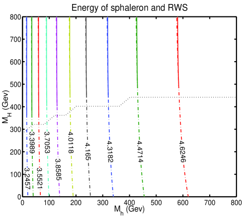
Figure 1: Contours in $M_{h}$, $M_{H}$ space of the energy of the sphaleron (dashes),and of the RWS (solid), in units of $M_{W}/\alpha_{W}$. Below the dotted line the sphaleron is the only solution. Above the dotted line, both solutions exist. The input parameters are $\tan\beta=6$ with all other parameters zero.

Figure 2: Contours in $M_{h}$, $M_{H}$ space of the eigenvalue in units of $M_{W}^{2}$. The top figure shows the most negative eigenvalule of the sphaleron (dashes), and of the RWS (solid). The bottom figure shows the second most negative eigenvalue of the sphaleron. Below the dotted line the sphaleron is the only solution. Above the dotted line, both solutions exist. The input parameters are $\tan\beta=6$ with all other parameters zero.

Figs. 1–3 show contours in the $M_{h}$ and $M_{H}$ plane. The contours are respectively of energy (Fig. 1), most negative eigenvalue and second most negative eigenvalue (Fig. 2), and $n_{CS}$ (Fig. 3) of the sphaleron and relative winding sphaleron. When we show equal contours of both solutions the sphalerons are shown as dashes, and the RWS as solid. Below the black horizontal dotted line, shown on all four contour plots, only the sphaleron solution exists, above the black dotted line both solutions exist. The sphaleron never develops a third negative eigenvalue, nor the RWS a second negative eigenvalue. The solutions maintained exact spherical symmetry: $V_{2}$ was zero throughout; this was expected as both $\theta_{CP}=0$, and $M_{A}=M_{H^{\pm}}=0$. These contours are from the same potential as used by BTT [26] and contain some of the parameter space they scanned. Where we overlap we agree with their results, and we confirm their observation that the second negative eigenvalue appears when one of the Higgs has a largeish mass, ($M_{H}\sim 5M_{W}$). For low values of this heavier mass the lighter Higgs needs to be as light as possible; i.e. for the existence of relative winding sphalerons it is preferable to have the two Higgs masses, $M_{h}$ and $M_{H}$, well separated.

Fig. 1 shows both the energy of the sphaleron and the energy of the RWS, there is almost no difference between their energies, and the energy depends mainly on the mass of the lighter Higgs. Figure 2 shows the most negative eigenvalue of both the sphaleron and RWS, and we see that there is a large difference between the values of negative eigenvalues for the different solutions; the negative eigenvalue of the sphaleron can be double that for the relative winding sphaleron for the same point in parameter space. Fig. 2 also shows the second negative eigenvalue of the sphaleron. The second most negative eigenvalue belongs to the perturbation which leads to the RW sphaleron in configuration space.

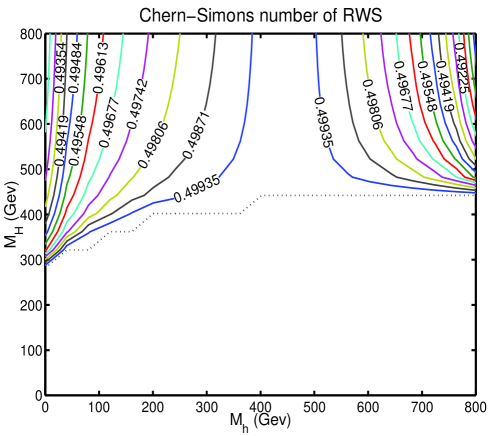
Figure 3: Contours in $M_{h}$, $M_{H}$ space of the Chern-Simons number of the RWS. Below the dotted line only the sphaleron solution exists, with $n_{CS}=1/2$. The input parameters are $\tan\beta=6$ with all other parameters zero.

Looking at Fig. 3 we see that the Chern-Simons number of the RW sphaleron is generally not a half. There is a line in the contour space where $n_{CS}=1/2$. This occurs, for $\tan\beta=1$, along the line of $M_{h}=M_{H}$, and shifts in the contour plane for different values of $\tan\beta$. We have only shown here solutions with $n_{CS}\leq 1/2$. Each of these solutions with $n_{CS}\leq 1/2$ has a $P$ conjugate partner, with Chern-Simons $n_{CS}^{con}\geq 1/2$, such that $n_{CS}+n_{CS}^{con}=1$.

5.2 No $CP$ violation, $M_{A}=3M_{W}$, $M_{H^{\pm}}=2M_{W}$

Figs. 4–6 show contours in $M_{h}$, $M_{H}$ space of energy (Fig. 4), most negative eigenvalue of the sphaleron and RWS, (Fig. 5 top), and second most negative eigenvalue of the sphaleron (Fig. 5 bottom), and $n_{CS}$ (Fig. 6) of the sphaleron and the relative winding sphaleron. Again when both solutions are shown the sphaleron is dashes, and the RWS solid.

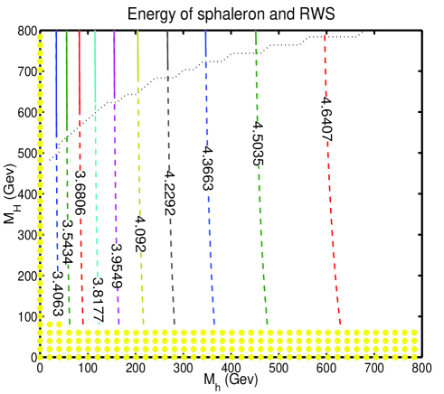
Figure 4: Contours in $M_{h}$, $M_{H}$ space of the energy of the sphaleron (dashes),and of the RWS (solid), in units of $M_{W}/\alpha_{W}$. Below the dotted line the sphaleron is the only solution, while above, both solutions exist. For the dotted area the potential is unbounded. The input parameters are $\tan\beta=6$, $M_{A}=241$ GeV, $M_{H^{\pm}}=161$ GeV, and $\lambda_{3}=-0.05$.

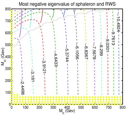
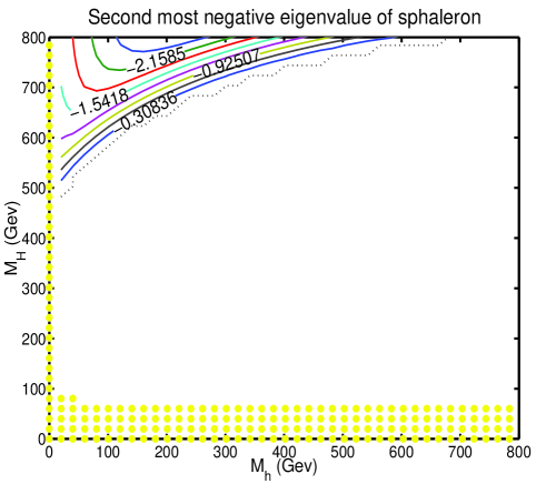
Figure 5: Contours in $M_{h}$, $M_{H}$ space of eigenvalues in units of $M_{W}^{2}$. The top figure shows the most negative eigenvalue of the sphaleron (dashes), and of the RW sphaleron (solid). The bottom figure shows the second most negative eigenvalue of the sphaleron. Below the dotted line the sphaleron is the only solution. Above the dotted line, both solutions exist. For the dotted region the potential is unbounded. The input parameters are $\tan\beta=6$, $M_{A}=241$ GeV, $M_{H^{\pm}}=161$ GeV, and $\lambda_{3}=-0.05$.

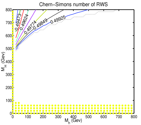
Figure 6: Contours in $M_{h}$, $M_{H}$ space of the Chern-Simons number of the RW sphaleron. Below the dotted line only the sphaleron solution exists, with $n_{CS}=0.5$. For the dotted region the potential is unbounded. The input parameters are $\tan\beta=6$, $M_{A}=241$ GeV, $M_{H^{\pm}}=161$ GeV, and $\lambda_{3}=-0.05$.

For these figures we took $M_{A}=241$ GeV, $M_{H^{\pm}}=161$ GeV, again with no explicit $CP$ violation. We set the parameters $\lambda_{3}=-0.05$, and $\tan\beta=6$, and scanned through $M_{h}$ and $M_{H}$ between 0 and 800 GeV, with 20 GeV increments. Again below the black dotted line, shown on all four contour plots, only the sphaleron solution exits, while above both solutions exist. We see that the RW sphaleron solutions still persist for a large region of the parameter space. The dotted region at low $M_{H}$ was unbounded according to Eqs. 39 and 40. These solutions did not maintain exact spherical symmetry corresponding to $V_{2}=0$, but the maximum value of energy due to the $V_{2}$ term was 0.6% of the energy due to $V_{0}$.

The solutions have the same general features as those at zero $M_{A}$ and $M_{H^{\pm}}$: the RW sphaleron appears at widely separated $M_{H}$ and $M_{h}$. While the energies of the two solutions in Fig. 4 are almost indistinguishable, the most negative eigenvalue (Fig. 5 top), of the sphaleron can be double that of the RW sphaleron. We show the value of the second most negative eigenvalue of the sphaleron in Fig. 5 (bottom). The sphaleron never developed a third negative eigenvalue, nor the RW sphaleron a second negative eigenvalue. In Fig. 6 we show the Chern-Simons number of the RW sphaleron, and again for every solution shown with $n_{CS}=1/2-\nu$ there is a $P$ conjugate solution with $n^{con}_{CS}=1/2+\nu$.

5.3 $CP$ violation, $M_{A}=8M_{W}$, $M_{H^{\pm}}=2M_{W}$

Figs. 7–9 show contours in $M_{h}$, $M_{H}$ space of energy and second negative eigenvalue (Fig. 7), most negative eigenvalue (Figs. 8) and Chern-Simons number (Fig. 9) of the sphaleron and relative winding sphaleron. Sphaleron contours are shown as dashed lines and RW sphaleron contours as solid when present on the same graph.

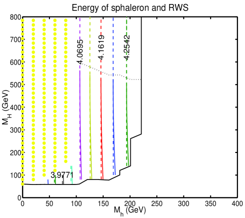
Figure 7: Top: contours in $M_{h}$, $M_{H}$ space of energy in units of $M_{W}/\alpha_{W}$ of the sphaleron (dashes),and of the RW sphaleron (solid). Bottom: contours in $M_{h}$, $M_{H}$ space of second negative eigenvalue ($M_{W}^{2}$) of the sphaleron. Above the dotted line the sphaleron is the only solution, while below both solutions exist. For the blank area Eq. 10 is not the global minimum. For the dotted area the potential is unbounded. The input parameters are $\theta_{CP}=0.49\pi$, $\phi=0.1\pi$, $\psi=0.0$, $M_{A}=643$ GeV, $M_{H^{\pm}}=161$ GeV, and $\lambda_{3}$=3.0. $\tan\beta$=3.1.

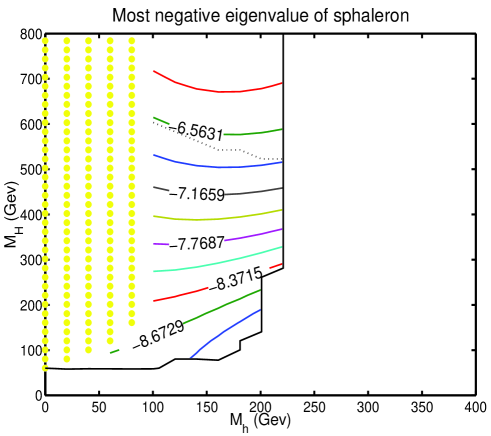
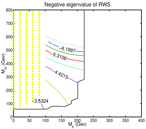
Figure 8: Contours in $M_{h}$, $M_{H}$ space of the most negative eigenvalue ($M_{W}^{2}$) of the sphaleron (top) and of the relative winding sphaleron (bottom). Above the dotted line the sphaleron is the only solution, while below both solutions exist. For the blank area Eq. 10 is not the global minimum. For the dotted area the potential is unbounded. The input parameters are $\theta_{CP}$=0.49$\pi$, $\phi$=0.1$\pi$, $\psi$=0.0, $M_{A}=643$ GeV, $M_{H^{\pm}}=161$ GeV, and $\lambda_{3}$=3.0. $\tan\beta$=3.1.

Figure 9: Contours in $M_{h}$, $M_{H}$ space of the Chern-Simons number of the RWS. Above the dotted line only the sphaleron solution exists, with $n_{CS}=1/2$. For the blank area Eq. 10 is not the global minimum. For the dotted area the potential is unbounded. The input parameters are $\theta_{CP}$=0.49$\pi$, $\phi$=0.1$\pi$, $\psi$=0.0, $M_{A}=643$ GeV, $M_{H^{\pm}}=161$ GeV, and $\lambda_{3}$=3.0. $\tan\beta$=3.1.

For these figures we took $M_{A}=643$ GeV, $M_{H^{\pm}}=161$ GeV, this time with $CP$ violation: $\theta_{CP}=0.49\pi$. The remaining parameters were $\phi=0.1\pi$, $\psi$=0.0, and $\lambda_{3}$=3.0, giving $\tan\beta$=3.1. We scanned through $M_{h}$ between 0 and 400 GeV, and $M_{H}$ between 0 and 800 GeV, with 20 GeV increments. The dotted region at low $M_{h}$ was unbounded according to Eqs. 39 and 40, and for the white out area, surrounded by the solid black line, the minimum of Eq. 10 was not the global minimum.

As with the previous contour plots, a large region of parameter space contained relative winding sphalerons. For these input parameters, though, due to the large $CP$ violating mixing angle, the role of the large Higgs mass $M_{H}$ is taken on by $M_{A}$. Since, from previous contour plots, the relative winding sphaleron solution prefers regions of parameter space where there is a large separation in values of the heaviest (in this case the $M_{A}$) and the lightest (in this case $M_{h}$, and $M_{H}$) Higgs masses, the relative winding sphaleron solultions exist for the lower part of the contour plot, and not the upper part. Referring to Figs. 7–9: above the black dotted line the sphaleron is the only solution, while below the black dotted line both the sphaleron and the relative winding sphaleron exist, this is opposite to the behaviour in the absence of $CP$ violation.

From Fig. 7 (top) the energy of the two solutions is as before almost the same. The second negative eigenvalue of the sphaleron is shown in the lower half of Fig. 7. The sphaleron does not develop a third negative eigenvalue, nor the RW sphaleron a second negative eigenvalue. We show the most negative eigenvalue of the sphaleron and the RW sphaleron (Fig. 8) on separate graphs, and again their respective negative eigenvalues can be very different at the same point in the contour plane. We then show the Chern-Simons numbers for the RW sphaleron in Fig. 9. Note that we only show solutions with $n_{CS}\leq 1/2$: again, there are parity conjugate partners to each of these RW sphalerons, and the $n_{CS}$ of the RW sphaleron and of its parity partner add up to one.

There is no breaking in the degeneracy of the relative winding sphaleron pairs in energy, eigenvalues, or absolute difference from 1/2 of Chern-Simons number, due to the presence of $CP$ violation. The solutions are not exactly spherically symmetric, and have non zero values for all three of $K_{1}$, $V_{1}$, and $V_{2}$. The values of $K_{1}$, $V_{1}$, and $V_{2}$ as a percentage of the Higgs potential energy are each never more than 0.5 %.

5.4 MSSM parameter space

Next we scan through tree level MSSM parameter space. Fig. 10 shows the scan in $M_{A}$, $\tan\beta$ space. Fig. 11 shows the scan in $M_{h}$, $M_{H}$ space. We plot contours of energy (top) and negative eigenvalue (bottom) for each of these scans.

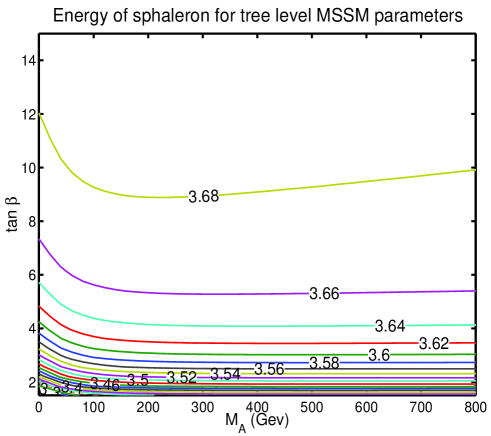
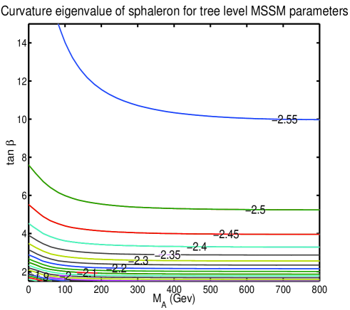
Figure 10: Contours in $M_{A}$, $\tan\beta$ space of the sphaleron for tree level MSSM parameters. The top figure shows energy ($M_{W}/\alpha_{W}$) of the sphaleron. The bottom figure shows negative curvature eignevalue ($M_{W}^{2}$) of the sphaleron.

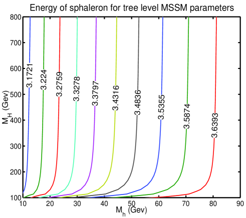
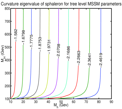
Figure 11: Contours in $M_{h}$, $M_{H}$ space of the energy ($M_{W}/\alpha_{W}$) of the sphaleron for tree level MSSM parameters. The top figure shows energy ($M_{W}/\alpha_{W}$) of the sphaleron. The bottom figure shows negative curvature eignevalue ($M_{W}^{2}$) of the sphaleron.

For the range of parameters we show the sphaleron did not develop a second negative eigenvalue. There was no departure from spherical symmetry, as only the $a_{\alpha}$ field of the Higgs ansatz and the $\beta$ field of the gauge ansatz were ever non-zero. From these four contours (Figs. 10 and 11) we agree with the general result of [28] that the energy of the sphaleron is sensitive to mainly $M_{h}$ and $\tan\beta$, although their results should be more accurate as they included 1-loop radiative corrections. There were no relative winding sphalerons for the range of parameters explored.

5.5 Sphaleron energy and $CP$ violation

We recall that a $CP$ violating mixing angle can have a large effect on the properties of the sphaleron. Here (Fig. 12) we scan through $M_{h}$, $\theta_{CP}$ space and show the energy of the sphaleron and the negative eigenvalue of the sphaleron for input parmaters $\phi$=0.125$\pi$, $\psi$=0.0, $M_{H}=110$ GeV, $M_{A}=500$ GeV, $M_{H^{\pm}}=500$ GeV, and $\lambda_{3}$=0.0, these give $\tan\beta$=2.4. For the dotted region at low $M_{h}$ the potential was unbounded, and for the blank region, bordered by the solid black line, the minimum of Eq. 10 was not the global minimum of the static energy functional. For this region of parameter space the sphaleron never developed a second negative curvature eigenvalue.

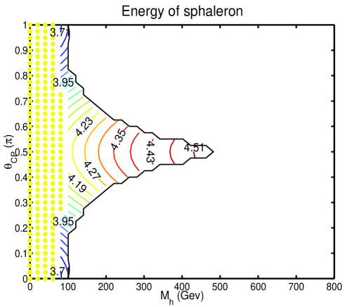
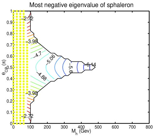
Figure 12: Top: contours in $M_{h}$, $\theta_{CP}$ space of the energy ($M_{w}/\alpha_{w}$) of sphaleron, and bottom: of the negative eigenvalue of the sphaleron ($M_{W}^{2}$). For this region of parameter space the sphaleron is the only solution. For the blank region Eq. 10 is not the global minimum. For the dotted region the potential is unbounded. The input parameters are $\phi$=0.125$\pi$, $\psi$=0.0, $M_{H}=110$ GeV, $M_{A}=500$ GeV, $M_{H^{\pm}}=500$ GeV, and $\lambda_{3}$=0.0. $\tan\beta$=2.4.

The energy of the sphaleron (Fig. 12: top) is dependent upon the value of the $CP$ violating mixing angle, and changes by about fourteen percent as the mixing angle varies between its minimum and its maximum. The energy is, in the presence of $CP$ violation, still sensitive to the lightest Higgs mass.

The negative eigenvalue (Fig. 12: bottom) also has this strong dependence on the $CP$ violating mixing angle, with an increase of over fifty percent as the mixing angle varies. Also the dependence on $M_{h}$, although not as dramatic as the effect of $CP$ violation, is still present.

5.6 Field profiles

5.6.1 Sphaleron and RW sphaleron

Next we show the field profiles for the sphaleron, relative winding sphaleron, and conjugate relative winding sphaleron for a point in the contour plot of Section 5.3 corresponding to a $CP$ violating theory with $M_{A}=8M_{W}$, $M_{H^{\pm}}=2M_{W}$, $M_{h}=1.25M_{W}$, and $M_{H}=1.5M_{W}$. We recall that the mixing angles were $\theta_{CP}$=0.49$\pi$, $\phi$=0.1$\pi$, $\psi$=0.0, and the coupling $\lambda_{3}=3.0$.

Before we proceed we check whether this point in parameter space is phenomenologically viable at zero temperature, as $M_{h}=1.25M_{W}$ is ruled out if the $hZZ$ coupling is too large. We calculate the couplings $g_{hZZ}$, $g_{HZZ}$, and $g_{AZZ}$ according to [43] using the values of input parameters used in Figs. 13–16, and compare them with the latest particle data [44].

Using

$$g_{hZZ} = D[1,1]\cos\beta+D[2,1]\sin\beta$$ (81)

$$g_{HZZ} = D[1,2]\cos\beta+D[2,2]\sin\beta$$ (82)

$$g_{AZZ} = D[1,3]\cos\beta+D[2,3]\sin\beta$$ (83)

where $D$ is given by Eq. 16, we obtain, for the paramaters of figures 13-16

$$g^{2}_{hZZ} = 0.081$$ (84)

$$g^{2}_{HZZ} = 0.824$$ (85)

$$g^{2}_{AZZ} = 0.095$$ (86)

which for masses $M_{h}=101$ GeV, $M_{H}=121$ GeV, and $M_{A}=643$ GeV are with in experimental bounds. Although we have labelled the Higgses with subscripts $h$, $H$, and $A$; because of the values of the mixings $\phi=0.1\pi$, $\theta_{CP}=0.49\pi$, $\psi=0.0$, while the particle with subscript $h$ is $CP$ even, those with subscript $H$, and $A$ are a mix of $CP$ even and $CP$ odd.

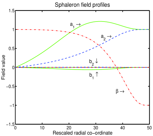
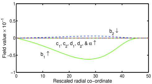
Figure 13: The sphaleron field profiles (top), and the profiles for $b_{1}$ and $b_{2}$ in more detail (bottom). $c_{\alpha}=d_{\alpha}=\alpha=0$. This configuration has energy=$4.053$ $M_{W}/\alpha_{W}$, $n_{CS}$=1/2, and two negative curvature eigenvalues $-8.696M_{W}^{2}$, and $-1.754M_{W}^{2}$. Input parameters are: $\theta_{CP}$=0.49$\pi$, $\phi$=0.1$\pi$, $\psi$=0.0, $M_{h}=101$ GeV, $M_{H}=121$ GeV, $M_{A}=643$ GeV, $M_{H^{\pm}}=161$ GeV, and $\lambda_{3}$=3.0. These give $\tan\beta$=3.1, $\lambda_{1}=26.29$, $\lambda_{2}=-2.59$, $\lambda_{+}=0.91$, $\lambda_{4}=0.85$, $\chi_{1}=0.42$, and $\chi_{2}=0.41$.

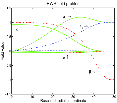
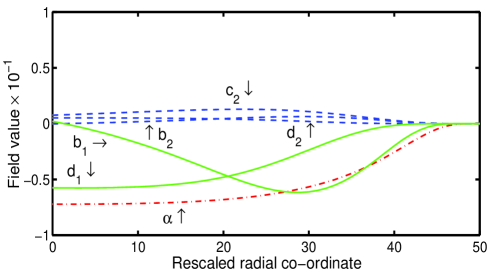
Figure 14: The RW sphaleron field profiles (top) and the profiles for $b_{1}$, $b_{2}$, $c_{2}$, $d_{1}$, $d_{2}$, and $\alpha$ in more detail (bottom). This configuration has energy=$4.047$ $M_{W}/\alpha_{W}$, $n_{CS}$=0.478, and one negative curvature eigenvalue $-3.637M_{W}^{2}$. Input parameters are: $\theta_{CP}$=0.49$\pi$, $\phi$=0.1$\pi$, $\psi$=0.0, $M_{h}=101$ GeV, $M_{H}=121$ GeV, $M_{A}=643$ GeV, $M_{H^{\pm}}=161$ GeV, and $\lambda_{3}$=3.0. These give $\tan\beta$=3.1, $\lambda_{1}=26.29$, $\lambda_{2}=-2.59$, $\lambda_{+}=0.91$, $\lambda_{4}=0.85$, $\chi_{1}=0.42$, and $\chi_{2}=0.41$.

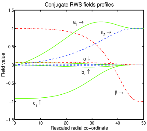
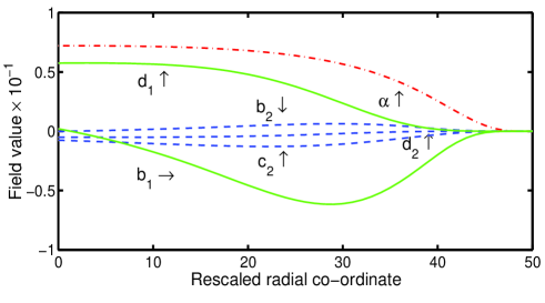
Figure 15: The conjugate RW sphaleron field profiles (top), and the profiles for $b_{1}$, $b_{2}$, $c_{2}$, $d_{1}$, $d_{2}$, and $\alpha$ in more detail (bottom). This configuration has energy=$4.047$ $M_{W}/\alpha_{W}$, $n_{CS}$=0.522, and one negative curvature eigenvalue $-3.637M_{W}^{2}$. Input parameters are: $\theta_{CP}$=0.49$\pi$, $\phi$=0.1$\pi$, $\psi$=0.0, $M_{h}=101$ GeV, $M_{H}=121$ GeV, $M_{A}=643$ GeV, $M_{H^{\pm}}=161$ GeV, and $\lambda_{3}$=3.0. These give $\tan\beta$=3.1, $\lambda_{1}=26.29$, $\lambda_{2}=-2.59$, $\lambda_{+}=0.91$, $\lambda_{4}=0.85$, $\chi_{1}=0.42$, and $\chi_{2}=0.41$.

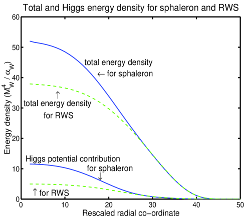
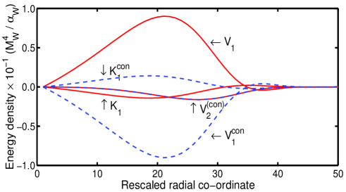
Figure 16: The top of the figure shows the total and the Higgs potential contribution to energy density in units of $M_{W}^{4}/\alpha_{W}$ for the sphaleron (solid) and the RWS (dashes). The bottom figure shows $K_{1}$, $V_{1}$, and $V_{2}$ for the RWS (solid) and its conjugate (dashes) in the same units. Both $K_{1}$ and $V_{1}$ are equal to their values for conjugate solutions, but have opposite sign. $V_{2}$ is equal to its value for the conjugate solution. Input parameters are: $\theta_{CP}$=0.49$\pi$, $\phi$=0.1$\pi$, $\psi$=0.0, $M_{h}=101$ GeV, $M_{H}=121$ GeV, $M_{A}=643$ GeV, $M_{H^{\pm}}=161$ GeV, and $\lambda_{3}$=3.0. These give $\tan\beta$=3.1, $\lambda_{1}=26.29$, $\lambda_{2}=-2.59$, $\lambda_{+}=0.91$, $\lambda_{4}=0.85$, $\chi_{1}=0.42$, and $\chi_{2}=0.41$.

We then plot the energy density of the two types of solution, and the values of $K_{1}$, $V_{1}$, and $V_{2}$ as a function of the rescaled radial co-ordinate for the sphaleron, RW sphaleron, and conjugate RW sphaleron. We recall that the departure of $K_{1}$, $V_{1}$, and $V_{2}$ from zero signals the breakdown of the spherically symmetric ansatz, and their size relative to the total energy density indicates the seriousness of the breakdown.

It is convenient to plot the field values rescaled according to

$$f_{G}=\frac{f_{G}}{\sqrt{2}},~{}~{}~{}~{}f_{H}=\frac{\upsilon}{\upsilon_{\alpha}}\frac{f_{H}}{2},$$ (87)

as then the asymptotic values are either 0 or $\pm 1$.

The ordinary sphaleron field profiles are plotted in Fig. 13 as a function of the rescaled radial points. The solution has non zero values of $a_{\alpha}$, $b_{\alpha}$, and $\beta$ as expected for a field configuration that preserves $P$ but violates $C$, due to the presence of a $C$ violating parameter in the potential. The sphaleron has Chern-Simons number 1/2, two negative eigenvalues (-8.696 $M^{2}_{W}$, and -1.754 $M^{2}_{W}$), and has energy $4.053M_{W}/\alpha_{W}$.

The relative winding sphaleron field configurations, shown in Fig. 14, have non zero values for all fields. The solution violates $P$ spontaneously and $C$ explicitly, and violates the combination $CP$. It has one negative eigenvalue (-3.637 $M^{2}_{W}$), energy less than its ordinary sphaleron ($4.047M_{W}/\alpha_{W}$), and Chern-Simons number 0.478. Its parity congugate partner, shown in Figure 15, has field profiles identical to a $P$ transformation of the RWS: that is $c_{\alpha}\rightarrow-c_{\alpha}$, $d_{\alpha}\rightarrow-d_{\alpha}$, and $\alpha\rightarrow-\alpha$, with all other fields remaining unchanged. The solution has identical energy, and eigenvalue to its $P$ conjugate solution, and its Chern-Simons number is 0.522.

Next we show (Fig. 16: top) the energy density of the sphaleron, and the RW sphaleron, and in detail (Fig. 16: bottom) the values of $K_{1}$, $V_{1}$, and $V_{2}$ for the RWS in units of energy density. $K_{1}$ and $V_{1}$ are equal in value, but opposite in sign for the conjugate pair, $V_{2}$ is equal in value and equal in sign. These deviations from spherical symmetry are of order one part in $10^{3}$ for these values of parameters.

5.6.2 Bisphaleron

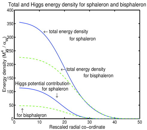
Figure 17: The top figure shows total and Higgs potential contribution to energy density ($M_{W}^{4}/\alpha_{W}$) for the sphaleron (solid) and the bisphaleron (dashes). The bottom figure shows $V_{2}$ for the bisphaleron solution and its conjugate. $V_{2}$ for both the bisphaleron and conjugate solution are equal. Input parameters are: $\tan\beta$=6.0, $\theta_{CP}$=0.0, $\phi$=0.0, $\psi$=0.0, $M_{h}$=15.0$M_{W}$, $M_{H}$=17.0$M_{W}$, $M_{A}$=2.0$M_{W}$, $M_{H^{\pm}}$=3.0$M_{W}$, and $\lambda_{3}$=-0.1.

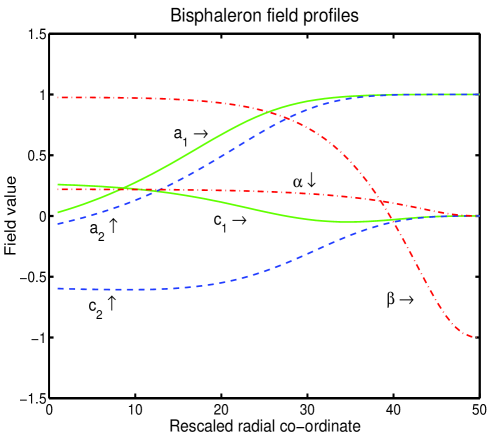
Figure 18: The bisphaleron field profiles for $\tan\beta$=6.0, $M_{h}$=15.0$M_{W}$, $M_{H}$=17.0$M_{W}$, $M_{A}$=2.0$M_{W}$, $M_{H^{\pm}}=3.0M_{W}$ and $\lambda_{3}$=-0.1. It has energy=$4.932$ $M_{W}/\alpha_{W}$, $n_{CS}$=0.569, two negative curvature eigenvalues $-11.915M_{W}^{2}$, and $-6.788M_{W}^{2}$. Its conjugate partner is the identical solution under $P$ conjugation ($\alpha\rightarrow-\alpha$), and has $n_{CS}$=0.431.

For completeness we detail the bisphaleron fields profiles for non zero $M_{A}$ and $M_{H^{\pm}}$, and show their departure from spherical symmetry. Figs. 17 and 18 concern this bisphaleron. We have chosen masses which are perhaps unrealistically large, in order to reach the part of parameter space where the bisphaleron exists: $\tan\beta$=6.0, $M_{h}$=15.0$M_{W}$, $M_{H}$=17.0$M_{W}$, $M_{A}$=2.0$M_{W}$, $M_{H^{\pm}}$=3.0$M_{W}$ and $\lambda_{3}$=-0.1, with no CP violation. For these input parameters $\lambda_{1}=567.6$, $\lambda_{2}=12.4$, $\lambda_{+}=0.627$, $\lambda_{4}=1.923$, $\chi_{1}=-0.227$, and $\chi_{2}=0.0$.

The energy density and departure from spherical symmetry are shown in Figure 17. The $CP$ invariance means that $b_{\alpha}=d_{\alpha}=0$, and hence $K_{1}$ and $V_{1}$ vanish. The departure from spherical symmetry is entirely in the $V_{2}$ term shown in units of energy density ($M_{W}^{4}/\alpha_{W}$) in the lower half of Fig. 17. The departure from spherical symmetry is of order 1 part in $10^{4}$.

The configuration in Fig. 18 has energy=$4.932$ $M_{W}/\alpha_{W}$, $n_{CS}$=0.569, it has two negative curvature eigenvalues -11.915 $M_{W}^{2}$, and -6.788 $M_{W}^{2}$. Its associated sphaleron has energy=$4.943$ $M_{W}/\alpha_{W}$ with $n_{CS}$=1/2, and three negative curvature eigenvalues $-23.823M_{W}^{2}$, $-13.249M_{W}^{2}$, and $-0.933M_{W}^{2}$. Its conjugate bisphaleron has identical energy, and negative curvature eigenvalues, but $n_{CS}$=0.431; so again the $n_{CS}$ of the bisphaleron and its conjugate add to one.

6 Conclusions

In this paper we have made a thorough study of the properties of sphalerons in two Higgs doublet SU(2) gauge theories. Using a spherically symmetric approximation, we have performed scans in the physical parameter space defined by the masses and mixing angles of the Higgs particles, recording the energy, lowest eigenvalues, and the Chern-Simons number, with results recorded in Figs. 1–12. We have also shown the profiles of the fields of our ansatz for selected solutions in Figs. 13–18.

We can draw a number of broad conclusions from these results. Firstly, for a wide range of parameters, the minimum energy sphaleron is not the natural generalisation of the Klinkhamer-Manton sphaleron [22] with vanishing Higgs fields at the origin, but a parity violating pair of relative winding (RW) sphalerons, first identified by Bachas, Tinyakov, and Tomaras [26]. These are related to the bisphalerons or deformed sphalerons found in one doublet models by Yaffe [24] and Kunz and Brihaye [23], but are specific to two Higgs doublet models. This pair was always degenerate in energy, as is to be expected from a parity conserving Lagarangian. This degeneracy is lifted when Standard Model fermions are included [45].

The favoured regions of parameter space for RW sphalerons to exist are those where there is a large difference in the masses of the neutral Higgses. The mass of the heavier Higgs can be as low as $5M_{W}$. Bisphalerons appear at yet higher heavy Higgs masses, but were always more massive than the RW sphalerons in the parameter space we explored.

The appearance of extra sphaleron solutions is signalled by the ordinary sphaleron developing another negative eigenvalue: thus where the RW sphaleron exists the ordinary sphaleron has two negative eigenvalues, and three where the bisphaleron exists also. The lowest energy sphaleron must have exactly one negative eigenvalue. The numerically calculated eigenvalues of a solution not only aid its identification, but are important for accurate calculation of the baryon number violation rate: if the negative eigenvalue of the lowest energy sphaleron solution is $\omega_{-}^{2}$, then the rate is proportional to $|\omega_{-}|$ [34]. The difference between the most negative eigenvalue of the sphaleron and the negative eigenvalue of the RW sphaleron could be well over a factor of two.

The most important quantity for the calculation of the $B$ violation rate is normally the sphaleron energy. There is however very little difference in the energies of the ordinary and RW sphaleron: typically less than 1% in the range of parameters we surveyed. Thus the main contribution to the error in the rate from using the ordinary sphaleron comes from the negative eigenvalue. One must not only use the correct eigenvalue but also include a factor of two in the RW sphaleron rate, one for each of the two degenerate parity conjugate solutions. However, this leads only to logarithmic corrections to the sphaleron energy bound (1).

The most important parameter for the sphaleron energy was found to be the mass of the lightest Higgs, in accordance with previous studies. However, we were able to extend our work on the dependence of the energy on the $CP$ violating mixing angle $\theta_{CP}$ [33] to show that there was an strong dependence on this quantity as well, with the sphaleron energy varying by $\sim$ 15 % as $\theta_{CP}$ was adjusted through its allowed range. We note as well that we were unable to find a region of parameter space for which RW sphalerons existed over a wide range of $\theta_{CP}$, for which the potential was bounded, and for which Eq. 10 was the global minimum.

Although we used a spherically symmetric ansatz, we found that two Higgs doublet sphalerons are generically not spherically symmetric. This means that our results are approximate: however, the departure from spherical symmetry, as measured by the relative size of the symmetry violating terms in the static energy functional, was less than 0.2%, and so this is not a serious problem for the accuracy of our results. A larger correction is to be expected when one considers the full SU(2)$\times$U(1) theory at non-zero $\theta_{W}$, for which one also has to abandon the spherically symmetric ansatz and resort to an axially symmetric one instead [46].

Another source of error is the neglect of radiative and thermal corrections. Ideally one should work out the determinants of fluctuation matrices [35, 36, 37, 38]. One can also find solutions using the 1-loop finite temperature effective potential [28]. This is an implicit gradient expansion, neglecting finite temperature corrections to gradient terms, which turn out to be small [39]. Such computations are model-dependent: one first computes radiatively corrected couplings in the static energy functional, and then the sphaleron energy. Our approach decouples the computation of the radiative corrections, for we can take masses and angles to be their 1-loop corrected values. Although this neglects cubic terms and terms of dimension higher than 4 in the potential, it is an easy way of improving on the tree-level calculation, without sacrificing too much accuracy, as the contribution to the energy from the Higgs potential can be seen from Figs. 16 and 17 to be small.

Despite these sources of error, we can conclude the calculations of the sphaleron energy in $CP$ conserving models cannot safely be applied to $CP$ violating electroweak theories, and that the sphaleron bound on the mass of the lightest Higgs in $CP$ violating theories requires further investigation.

We wish to thank Mikko Laine and Neil McNair for helpful discussions. This work was conducted on the SGI Origin platform using COSMOS Consortium facilities, funded by HEFCE, PPARC and SGI. We acknowledge computing support from the Sussex High Performance Computing Initiative.

Appendix A Parametrization of two-doublet potentials

In Section 2.1 we wrote the two Higgs doublet potential as Eq. 9. Here we write two common forms of the most general two Higgs doublet potential. Firstly we write

$$V(\phi_{1},\phi_{2}) = m_{1}^{2}\phi_{1}^{\dagger}\phi_{1}+m_{2}^{2}\phi_{2}^{\dagger}\phi_{2}+m_{12}^{2}\phi_{1}^{\dagger}\phi_{2}+m_{12}^{2*}\phi_{2}^{\dagger}\phi_{1}$$ (88)

$$\ell_{1}(\phi_{1}^{\dagger}\phi_{1})^{2}+\ell_{2}(\phi_{2}^{\dagger}\phi_{2})^{2}+\ell_{3}\phi_{1}^{\dagger}\phi_{1}\phi_{2}^{\dagger}\phi_{2}+\ell_{4}\phi_{1}^{\dagger}\phi_{2}\phi_{2}^{\dagger}\phi_{1}$$

$$+\ell_{5}\phi_{1}^{\dagger}\phi_{2}\phi_{1}^{\dagger}\phi_{2}+\ell_{5}^{*}\phi_{2}^{\dagger}\phi_{1}\phi_{2}^{\dagger}\phi_{1}$$

$$+\ell_{6}\phi_{1}^{\dagger}\phi_{1}\phi_{1}^{\dagger}\phi_{2}+\ell_{6}^{*}\phi_{1}^{\dagger}\phi_{1}\phi_{2}^{\dagger}\phi_{1}$$

$$+\ell_{7}\phi_{2}^{\dagger}\phi_{2}\phi_{1}^{\dagger}\phi_{2}+\ell_{7}^{*}\phi_{2}^{\dagger}\phi_{2}\phi_{2}^{\dagger}\phi_{1},$$

where the only complex parameters are the $m_{12}^{2}$, $\ell_{5}$, $\ell_{6}$, and $\ell_{7}$. This potential has 14 independent parameters. Imposing the discrete symmetry $\phi_{1}\rightarrow\phi_{1}$, $\phi_{2}\rightarrow-\phi_{2}$ on dimension four terms will force $\ell_{6}=\ell_{7}=0$, and we have a potential with ten independent parameters.

Writing the same potential as

$$V(\phi_{1},\phi_{2}) = (\lambda_{1}+\lambda_{3})(\phi_{1}^{\dagger}\phi_{1}-\frac{\upsilon_{1}^{2}}{2})^{2}+(\lambda_{2}+\lambda_{3})(\phi_{2}^{\dagger}\phi_{2}-\frac{\upsilon_{2}^{2}}{2})^{2}$$ (89)

$$+2\lambda_{3}(\phi_{1}^{\dagger}\phi_{1}-\frac{\upsilon_{1}^{2}}{2})(\phi_{2}^{\dagger}\phi_{2}-\frac{\upsilon_{2}^{2}}{2})$$

$$+\lambda_{4}\left[\phi_{1}^{\dagger}\phi_{1}\phi_{2}^{\dagger}\phi_{2}-\mathrm{Re}^{2}(\phi_{1}^{\dagger}\phi_{2})-\mathrm{Im}^{2}(\phi_{1}^{\dagger}\phi_{2})\right]$$

$$+\lambda_{5}(\mathrm{Re}(\phi_{1}^{\dagger}\phi_{2})-\frac{\upsilon_{1}\upsilon_{2}}{2}\cos\xi)^{2}+\lambda_{6}(\mathrm{Im}(\phi_{1}^{\dagger}\phi_{2})-\frac{\upsilon_{1}\upsilon_{2}}{2}\sin\xi)^{2}$$

$$+\lambda_{7}(\mathrm{Re}(\phi_{1}^{\dagger}\phi_{2})-\frac{\upsilon_{1}\upsilon_{2}}{2}\cos\xi)(\mathrm{Im}(\phi_{1}^{\dagger}\phi_{2})-\frac{\upsilon_{1}\upsilon_{2}}{2}\sin\xi)$$

$$+\mu_{1}(\phi_{1}^{\dagger}\phi_{1}-\frac{\upsilon_{1}^{2}}{2})(\mathrm{Re}(\phi_{1}^{\dagger}\phi_{2})-\frac{\upsilon_{1}\upsilon_{2}}{2}\cos\xi)$$

$$+\mu_{2}(\phi_{1}^{\dagger}\phi_{1}-\frac{\upsilon_{1}^{2}}{2})(\mathrm{Im}(\phi_{1}^{\dagger}\phi_{2})-\frac{\upsilon_{1}\upsilon_{2}}{2}\sin\xi)$$

$$+\mu_{3}(\phi_{2}^{\dagger}\phi_{2}-\frac{\upsilon_{2}^{2}}{2})(\mathrm{Re}(\phi_{1}^{\dagger}\phi_{2})-\frac{\upsilon_{1}\upsilon_{2}}{2}\cos\xi)$$

$$+\mu_{4}(\phi_{2}^{\dagger}\phi_{2}-\frac{\upsilon_{2}^{2}}{2})(\mathrm{Im}(\phi_{1}^{\dagger}\phi_{2})-\frac{\upsilon_{1}\upsilon_{2}}{2}\sin\xi),$$

where all the parameters are real, we again have a potential with 14 independent parameters. Imposing $\phi_{1}\rightarrow\phi_{1}$, $\phi_{2}\rightarrow-\phi_{2}$ on dimension four terms we force four of these parameters $\mu_{1}=\mu_{2}=\mu_{3}=\mu_{4}=0$, and we have a ten parameter potential.

The advantage of writing the potential as Eq. 89 is that the three of the parameters of the potential are $\xi$, $\upsilon_{1}$, and $\upsilon_{2}$, and that the zero of the potential is

$$\phi_{\alpha}=\frac{\upsilon_{\alpha}}{\sqrt{2}}\left[\begin{array}[]{c}0\\ e^{i\varphi_{\alpha}}\end{array}\right],$$ (92)

where $\varphi_{1}=0$, and $\varphi_{2}=\xi$.

The relations between the parameters of Eq. 88 and those of Eq. 89 are

$$m_{1}^{2} = -(\lambda_{1}+\lambda_{3})\upsilon_{1}^{2}-\lambda_{3}\upsilon_{2}^{2}-\frac{\mu_{1}}{2}\upsilon_{1}\upsilon_{2}\cos\xi-\frac{\mu_{2}}{2}\upsilon_{1}\upsilon_{2}\sin\xi,$$ (93)

$$m_{2}^{2} = -(\lambda_{2}+\lambda_{3})\upsilon_{2}^{2}-\lambda_{3}\upsilon_{1}^{2}-\frac{\mu_{3}}{2}\upsilon_{1}\upsilon_{2}\cos\xi-\frac{\mu_{4}}{2}\upsilon_{1}\upsilon_{2}\sin\xi,$$ (94)

$$\mathrm{Re}(m_{12}^{2}) = -\frac{\lambda_{5}}{2}\upsilon_{1}\upsilon_{2}\cos\xi-\frac{\lambda_{7}}{4}\upsilon_{1}\upsilon_{2}\sin\xi-\frac{\mu_{1}}{2}\upsilon_{1}^{2}-\frac{\mu_{3}}{2}\upsilon_{2}^{2},$$ (95)

$$\mathrm{Im}(m_{12}^{2}) = -\frac{\lambda_{5}}{2}\upsilon_{1}\upsilon_{2}\sin\xi-\frac{\lambda_{7}}{4}\upsilon_{1}\upsilon_{2}\cos\xi-\frac{\mu_{2}}{2}\upsilon_{1}^{2}-\frac{\mu_{4}}{2}\upsilon_{2}^{2},$$ (96)

$$\ell_{1} = \lambda_{1}+\lambda_{3},$$ (97)

$$\ell_{2} = \lambda_{2}+\lambda_{3},$$ (98)

$$\ell_{3} = 2\lambda_{3}+\lambda_{4},$$ (99)

$$\ell_{4} = \frac{\lambda_{5}+\lambda_{6}}{2}-\lambda_{4},$$ (100)

$$\ell_{5} = \frac{1}{4}(\lambda_{5}-\lambda_{6}-i\lambda_{7}),$$ (101)

$$\ell_{6} = \frac{1}{2}(\mu_{1}-i\mu_{2}),$$ (102)

$$\ell_{7} = \frac{1}{2}(\mu_{3}-i\mu_{4}).$$ (103)

We are free to redefine the fields $\phi_{\alpha}$ of Eqs. 88 and 89. Rewriting Eq. 89 with $\phi_{\alpha}\rightarrow\phi_{\alpha}e^{i\varphi_{\alpha}}$ gives

$$V(\phi_{1},\phi_{2}) = (\lambda_{1}+\lambda_{3})(\phi_{1}^{\dagger}\phi_{1}-\frac{\upsilon_{1}^{2}}{2})^{2}+(\lambda_{2}+\lambda_{3})(\phi_{2}^{\dagger}\phi_{2}-\frac{\upsilon_{2}^{2}}{2})^{2}$$

$$+2\lambda_{3}(\phi_{1}^{\dagger}\phi_{1}-\frac{\upsilon_{1}^{2}}{2})(\phi_{2}^{\dagger}\phi_{2}-\frac{\upsilon_{2}^{2}}{2})$$

$$+\lambda_{4}\left[\phi_{1}^{\dagger}\phi_{1}\phi_{2}^{\dagger}\phi_{2}-\mathrm{Re}^{2}(\phi_{1}^{\dagger}\phi_{2})-\mathrm{Im}^{2}(\phi_{1}^{\dagger}\phi_{2})\right]$$

$$+(\lambda_{+}+\chi_{1})(\mathrm{Re}(\phi_{1}^{\dagger}\phi_{2})-\frac{\upsilon_{1}\upsilon_{2}}{2})^{2}+(\lambda_{+}-\chi_{1})\mathrm{Im}(\phi_{1}^{\dagger}\phi_{2})^{2}$$

$$+\chi_{2}(\mathrm{Re}(\phi_{1}^{\dagger}\phi_{2})-\frac{\upsilon_{1}\upsilon_{2}}{2})\mathrm{Im}(\phi_{1}^{\dagger}\phi_{2})$$

$$+\tilde{\mu_{1}}(\phi_{1}^{\dagger}\phi_{1}-\frac{\upsilon_{1}^{2}}{2})(\mathrm{Re}(\phi_{1}^{\dagger}\phi_{2})-\frac{\upsilon_{1}\upsilon_{2}}{2})+\tilde{\mu_{2}}(\phi_{1}^{\dagger}\phi_{1}-\frac{\upsilon_{1}^{2}}{2})\mathrm{Im}(\phi_{1}^{\dagger}\phi_{2})$$

$$+\tilde{\mu_{3}}(\phi_{2}^{\dagger}\phi_{2}-\frac{\upsilon_{2}^{2}}{2})(\mathrm{Re}(\phi_{1}^{\dagger}\phi_{2})-\frac{\upsilon_{1}\upsilon_{2}}{2})+\tilde{\mu_{4}}(\phi_{2}^{\dagger}\phi_{2}-\frac{\upsilon_{2}^{2}}{2})\mathrm{Im}(\phi_{1}^{\dagger}\phi_{2}),$$

and we now have a potential which is a function of 13 parameters, one less than both Eqs. 88 and 89. Where these new parmeters are in terms of those of Eq. 89

$$\lambda_{+} = \frac{1}{2}(\lambda_{5}+\lambda_{6}),$$ (106)

$$\lambda_{-} = \frac{1}{2}(\lambda_{5}-\lambda_{6}),$$ (107)

$$\chi_{1} = \frac{\lambda_{7}}{2}\sin 2\xi+\lambda_{-}\cos 2\xi,$$ (108)

$$\chi_{2} = \frac{\lambda_{7}}{2}\cos 2\xi-\lambda_{-}\sin 2\xi,$$ (109)

$$\tilde{\mu_{1}} = \mu_{1}\cos\xi+\mu_{2}\sin\xi,$$ (110)

$$\tilde{\mu_{2}} = -\mu_{1}\sin\xi+\mu_{2}\cos\xi,$$ (111)

$$\tilde{\mu_{3}} = \mu_{3}\cos\xi+\mu_{4}\sin\xi,$$ (112)

$$\tilde{\mu_{4}} = -\mu_{3}\sin\xi+\mu_{4}\cos\xi.$$ (113)

On imposing the discrete symmetry $\phi_{1}\rightarrow\phi_{1}$, $\phi_{2}\rightarrow-\phi_{2}$ on dimension four terms $\tilde{\mu_{1}}=\tilde{\mu_{1}}=\tilde{\mu_{1}}=\tilde{\mu_{1}}=0$, and we have a potential which is a function of nine parameters, again one less than the potentials of Eqs. 88 and 89 with the same symmetry imposed. This nine parameter potential is Eq. 9 of section 2.1 and is the potential we use throughout.

Appendix B Extrema of the potential

Extrema of the potential given in Eq. 9 occur at solutions to the four independent equations

$$\frac{\delta V(X_{i})}{\delta X_{i}}=0,$$ (115)

where $i=1,2,3,4,$ and $X_{i}$ are the $x_{1}$, $x_{2}$, $y_{2}$, and $z_{2}$ of

$$\phi_{1}=\frac{\upsilon_{1}}{\sqrt{2}}\left[\begin{array}[]{c}0\\ x_{1}\end{array}\right],~{}~{}~{}~{}~{}\phi_{2}=\frac{\upsilon_{2}}{\sqrt{2}}\left[\begin{array}[]{c}z_{2}\\ x_{2}+iy_{2}\end{array}\right].$$ (116)

A general bounded function of four variables with quartic and quadratic terms only can have up to $2^{4}$ minima.

The trivially found solutions to Eq. 115 are $x_{1}=\pm 1$, $x_{2}=\pm 1$, $y_{2}=z_{2}=0$ (i.e. Eq. 10), and $x_{1}=x_{2}=y_{2}=z_{2}=0$. The only other solution we were able to find analytically was

$$x_{1} = 0,$$

$$x_{2}^{2}+y_{2}^{2}+z_{2}^{2}-1 = \frac{\lambda_{3}}{(\lambda_{2}+\lambda_{3})\tan^{2}\beta},$$

$$x_{2} = \frac{-\chi_{2}}{(\lambda_{+}+\chi_{1})}y_{2},$$ (117)

these describe a circle with one zero eigenvalue, and potential energy

$$V=\frac{\upsilon_{1}^{2}\upsilon_{2}^{2}}{4}\left[\frac{\lambda_{1}\lambda_{2}+(\lambda_{1}+\lambda_{2})\lambda_{3}}{(\lambda_{2}+\lambda_{3})\tan^{2}\beta}+\lambda_{+}+\chi_{1}\right],$$ (118)

which may be less than zero for a potential obeying Eqs. 39, 40, and 44, and is a zero of the other terms of the static energy functional 48.

To find numerically the global minimum, we implemented two methods. Firstly, using the Maple extremisation routine extrema, we looked for an extremum of $V(X_{i})$ with negative energy somewhere in the chosen region of parameter space. As the vacuum in our parametrisation has zero energy, this meant it was not the global minimum. We used this solution as an initial configuration for a simple relaxation algorithm, which is equivalent to setting ${\cal E^{{}^{\prime\prime}}}$ of the Newton method (Eq. 57) to unity. We then scanned though parameter space relaxing to the global minimum at every point.

Our second method was to use an initial configuration of $X_{i}=0$, find the eigenvalues of the configuration, and add a perturbation in the direction of the most eigenfunction with the most negative eigenvalue. We then used the relaxation routine on this configuration. We did this for each point in parameter space, reinitialising to $X_{i}=0$ at each point.

Appendix C Static energy functional

On substituting the ansatz of Eqs. 45–47 into the Lagrangian 2 we obtain the static energy functional of Eq. 48. Here we give the form of $K_{0}$, $K_{1}$, $V_{0}$, $V_{1}$, and $V_{2}$ for the $C$ conserving ansatz and for the $C$ and $P$ violating ansatz.

In the absence of $C$ violation $F_{\alpha}=a_{\alpha}$ and $G_{\alpha}=c_{\alpha}$, and we have the usual ansatz of Ratra and Yaffee [42] where $K_{1}=V_{1}=0$ and $K_{0}$, $V_{0}$, and $V_{2}$ are

$$K_{0} = K^{D}_{0}+K^{G}_{0},$$ (121)

$$K^{D}_{0}=\frac{1}{2r^{2}}\bigg{[}a_{\alpha}^{{}^{\prime}2}r^{2}+c_{\alpha}^{{}^{\prime}2}r^{2}+\alpha^{{}^{\prime}2}+\beta^{{}^{\prime}2}\bigg{]},$$

$$K^{G}_{0}=\frac{1}{2r^{2}}\bigg{[}\frac{1}{4r^{2}}(\alpha^{2}+\beta^{2}-2)^{2}$$

$$\hskip 28.45274pt+\frac{1}{4}(a_{\alpha}^{2}+c_{\alpha}^{2})(\alpha^{2}+\beta^{2}+2)$$

$$\hskip 28.45274pt+\frac{\sqrt{2}\beta}{2}(a_{\alpha}^{2}-c_{\alpha}^{2})-\sqrt{2}\alpha a_{\alpha}c_{\alpha}\bigg{]},$$

$$V_{0} =\frac{\upsilon^{2}}{16M_{W}^{2}} \bigg{[}(\lambda_{1}+\lambda_{3})\left(a_{1}^{2}+c_{1}^{2}-4\cos^{2}\beta\right)^{2}$$ (122)

$$+(\lambda_{2}+\lambda_{3})\left(a_{2}^{2}+c_{2}^{2}-4\sin^{2}\beta\right)^{2}$$

$$+2\lambda_{3}\left(a_{1}^{2}+c_{1}^{2}-4\cos^{2}\beta\right)\left(a_{2}^{2}+c_{2}^{2}-4\sin^{2}\beta\right)$$

$$+\lambda_{4}\left(a_{1}c_{2}-a_{2}c_{1}\right)^{2}$$

$$+(\lambda_{+}+\chi_{1})\left(a_{1}a_{2}+c_{1}c_{2}-4\cos\beta\sin\beta\right)^{2}\bigg{]},$$

$$V_{2} =\frac{\upsilon^{2}}{16M_{W}^{2}} \bigg{[}(-\lambda_{4}+\lambda_{+}-\chi_{1})\left(a_{1}c_{2}-a_{2}c_{1}\right)^{2}\bigg{]}.$$ (123)

This ansatz will maintain spherical symmetry if $V_{2}=0$. The condition $V_{2}=0$ is met if $\lambda_{4}=\lambda_{+}-\chi_{1}$, or equivalently if $M_{H^{\pm}}=M_{A}$. In cases where $M_{H^{\pm}}\neq M_{A}$, the spherical symmetry of a field configuration will still be maintained if $a_{1}c_{2}=a_{2}c_{1}$, as the $V_{2}$ terms vanish from the energy density. The ordinary sphaleron comes into this class of configurations since $c_{1}=c_{2}=0$. However, it is still important to include this term as it affects the form of $\cal E^{{}^{\prime\prime}}$ used in Eq. 58 to calculate the curvature eigenvalues.

In the presence of $C$ violation $b_{\alpha}$ and $d_{\alpha}$ are no longer zero and $K_{0}$, $K_{1}$, $V_{0}$, $V_{1}$, and $V_{2}$ are

$$K_{0} = K^{D}_{0}+K^{G}_{0},$$ (126)

$$K^{D}_{0}=\frac{1}{2r^{2}}\bigg{[}a_{\alpha}^{{}^{\prime}2}r^{2}+b_{\alpha}^{{}^{\prime}2}r^{2}+c_{\alpha}^{{}^{\prime}2}r^{2}+d_{\alpha}^{{}^{\prime}2}r^{2}+\alpha^{{}^{\prime}2}+\beta^{{}^{\prime}2}\bigg{]},$$

$$K^{G}_{0}=\frac{1}{2r^{2}}\bigg{[}\frac{1}{4r^{2}}(\alpha^{2}+\beta^{2}-2)^{2}$$

$$\hskip 28.45274pt+\frac{1}{4}(a_{\alpha}^{2}+b_{\alpha}^{2}+c_{\alpha}^{2}+d_{\alpha}^{2})(\alpha^{2}+\beta^{2}+2)$$

$$\hskip 28.45274pt+\frac{\sqrt{2}\beta}{2}(a_{\alpha}^{2}+b_{\alpha}^{2}-c_{\alpha}^{2}-d_{\alpha}^{2})-\sqrt{2}\alpha(a_{\alpha}c_{\alpha}+b_{\alpha}d_{\alpha})\bigg{]},$$

$$K_{1} =\frac{1}{2r^{2}} \bigg{[}(a_{\alpha}^{{}^{\prime}}d_{\alpha}^{{}^{\prime}}-b_{\alpha}^{{}^{\prime}}c_{\alpha}^{{}^{\prime}})r^{2}+\frac{1}{4}(a_{\alpha}d_{\alpha}+b_{\alpha}c_{\alpha})(\alpha^{2}+\beta^{2}-2)\bigg{]},$$ (127)

$$V_{0} =\frac{\upsilon^{2}}{16M_{W}^{2}} \bigg{[}(\lambda_{1}+\lambda_{3})\left(a_{1}^{2}+b_{1}^{2}+c_{1}^{2}+d_{1}^{2}-4\cos^{2}\beta\right)^{2}$$

$$+(\lambda_{2}+\lambda_{3})\left(a_{2}^{2}+b_{2}^{2}+c_{2}^{2}+d_{2}^{2}-4\sin^{2}\beta\right)^{2}$$

$$+2\lambda_{3}\left(a_{1}^{2}+b_{1}^{2}+c_{1}^{2}+d_{1}^{2}-4\cos^{2}\beta\right)\left(a_{2}^{2}+b_{2}^{2}+c_{2}^{2}+d_{2}^{2}-4\sin^{2}\beta\right)$$

$$+\lambda_{4}\left(\left(a_{1}c_{2}-a_{2}c_{1}+b_{1}d_{2}-b_{2}d_{1}\right)^{2}\right.$$

$$\hskip 25.6073pt\left.+\left(a_{1}d_{2}+a_{2}d_{1}-b_{1}c_{2}-b_{2}c_{1}\right)^{2}-4\left(a_{1}d_{1}-b_{1}c_{1}\right)\left(a_{2}d_{2}-b_{2}c_{2}\right)\right)$$

$$+(\lambda_{+}+\chi_{1})\left(a_{1}a_{2}+b_{1}b_{2}+c_{1}c_{2}+d_{1}d_{2}-4\cos\beta\sin\beta\right)^{2}$$

$$+(\lambda_{+}-\chi_{1})\left(a_{1}b_{2}-a_{2}b_{1}+c_{1}d_{2}-c_{2}d_{1}\right)^{2}$$

$$+2\chi_{2}\left(a_{1}a_{2}+b_{1}b_{2}+c_{1}c_{2}+d_{1}d_{2}-4\cos\beta\sin\beta\right)\left(a_{1}b_{2}-a_{2}b_{1}+c_{1}d_{2}-c_{2}d_{1}\right)\bigg{]},$$

$$V_{1} =\frac{\upsilon^{2}}{16M_{W}^{2}} \bigg{[}4(\lambda_{1}+\lambda_{3})\left(a_{1}^{2}+b_{1}^{2}+c_{1}^{2}+d_{1}^{2}-4\cos^{2}\beta\right)\left(a_{1}d_{1}-b_{1}c_{1}\right)$$ (129)

$$+4(\lambda_{2}+\lambda_{3})\left(a_{2}^{2}+b_{2}^{2}+c_{2}^{2}+d_{2}^{2}-4\sin^{2}\beta\right)\left(a_{2}d_{2}-b_{2}c_{2}\right)$$

$$+4\lambda_{3}\left(\left(a_{1}^{2}+b_{1}^{2}+c_{1}^{2}+d_{1}^{2}-4\cos^{2}\beta\right)\left(a_{2}d_{2}-b_{2}c_{2}\right)\right.$$

$$\hskip 25.6073pt+\left.\left(a_{2}^{2}+b_{2}^{2}+c_{2}^{2}+d_{2}^{2}-4\sin^{2}\beta\right)\left(a_{1}d_{1}-b_{1}c_{1}\right)\right)$$

$$+2(\lambda_{+}+\chi_{1})\left(a_{1}a_{2}+b_{1}b_{2}+c_{1}c_{2}+d_{1}d_{2}-4\cos\beta\sin\beta\right)\left(a_{1}d_{2}+a_{2}d_{1}-b_{1}c_{2}-b_{2}c_{1}\right)$$

$$-2(\lambda_{+}-\chi_{1})\left(a_{1}b_{2}-a_{2}b_{1}+c_{1}d_{2}-c_{2}d_{1}\right)\left(a_{1}c_{2}-a_{2}c_{1}+b_{1}d_{2}-b_{2}d_{1}\right)$$

$$+2\chi_{2}\left[\left(a_{1}a_{2}+b_{1}b_{2}+c_{1}c_{2}+d_{1}d_{2}-4\cos\beta\sin\beta\right)\left(a_{1}c_{2}-a_{2}c_{1}+b_{1}d_{2}-b_{2}d_{1}\right)\right.$$

$$\hskip 25.6073pt-\left.\left(a_{1}b_{2}-a_{2}b_{1}+c_{1}d_{2}-c_{2}d_{1}\right)\left(a_{1}d_{2}+a_{2}d_{1}-b_{1}c_{2}-b_{2}c_{1}\right)\right]\bigg{]},$$

$$V_{2} =\frac{\upsilon^{2}}{16M_{W}^{2}} \bigg{[}4(\lambda_{1}+\lambda_{3})\left(a_{1}d_{1}-b_{1}c_{1}\right)^{2}$$ (130)

$$+4(\lambda_{2}+\lambda_{3})\left(a_{2}d_{2}-b_{2}c_{2}\right)^{2}$$

$$+8\lambda_{3}\left(a_{1}d_{1}-b_{1}c_{1}\right)\left(a_{2}d_{2}-b_{2}c_{2}\right)$$

$$-\lambda_{4}\left(\left(a_{1}c_{2}-a_{2}c_{1}+b_{1}d_{2}-b_{2}d_{1}\right)^{2}\right.$$

$$\hskip 25.6073pt\left.+\left(a_{1}d_{2}+a_{2}d_{1}-b_{1}c_{2}-b_{2}c_{1}\right)^{2}-4\left(a_{1}d_{1}-b_{1}c_{1}\right)\left(a_{2}d_{2}-b_{2}c_{2}\right)\right)$$

$$+(\lambda_{+}+\chi_{1})\left(a_{1}d_{2}+a_{2}d_{1}-b_{1}c_{2}-b_{2}c_{1}\right)^{2}$$

$$+(\lambda_{+}-\chi_{1})\left(a_{1}c_{2}-a_{2}c_{1}+b_{1}d_{2}-b_{2}d_{1}\right)^{2}$$

$$-2\chi_{2}\left(a_{1}d_{2}+a_{2}d_{1}-b_{1}c_{2}-b_{2}c_{1}\right)\left(a_{1}c_{2}-a_{2}c_{1}+b_{1}d_{2}-b_{2}d_{1}\right)\bigg{]}.$$

Appendix D Numerical scheme

To implement the scheme numerically, we discretise the $n$ fields into $N$ values $f_{Ai}$ in the range $0\leq r\leq R$. The values at the boundaries $f_{A0}$ and $f_{A(N-1)}$ are determined by the boundary conditions in a way which we specify below. Hence ${\cal E}^{{}^{\prime\prime}}$ is a $n(N-2)\times n(N-2)$ matrix, and $\delta f$ and ${\cal E}^{{}^{\prime}}$ are $n(N-2)$ column vectors.

To increase the accuracy of the solution while minimising the number of points $N$ we use a rescaled co-ordinate $s$, where

$$s=\frac{1}{\ln|C|}\ln\left[\frac{1+\mu r}{1+r}\right],\quad\mu=\frac{M_{max}}{M_{w}},\quad C=\frac{1+\mu R}{1+R}.$$ (131)

Here, $M_{max}$ is the maximum of [$M_{h}$, $M_{H}$, $M_{A}$, $M_{H^{\pm}}$], and for $M_{max}=M_{w}$ we used $M_{max}=1.01\times M_{w}$. We took $R=20M_{w}^{-1}$ and used $N=51$ points throughout. It is also convenient to define two new functions $X(s)$, $Y(s)$ through

$$X(s)\equiv\frac{ds}{dr} = \frac{1}{\ln|C|}\frac{1}{(\mu-1)}\frac{(C^{s}-\mu)^{2}}{C^{s}},$$ (132)

$$Y(s)\equiv\frac{dX}{ds} = \frac{1}{\mu-1}\frac{(C^{s}-\mu)(C^{s}+\mu)}{C^{s}}.$$ (133)

The first derivative of the energy ${\cal E}^{{}^{\prime}}$ may be split into Higgs and gauge parts

$${\cal E^{{}^{\prime}}}_{H} = -(Yr^{2}+2r)\frac{df_{H}}{ds}-Xr^{2}\frac{d^{2}f_{H}}{ds^{2}}+\frac{1}{X}\frac{d~{}}{df_{H}}\left[K^{G}_{0}+V_{0}+\frac{1}{3}V_{2}\right],$$ (134)

$${\cal E^{{}^{\prime}}}_{G} = -Y\frac{df_{G}}{ds}-X\frac{d^{2}f_{G}}{ds^{2}}+\frac{1}{X}\frac{d~{}}{df_{G}}\left[K^{G}_{0}+V_{0}+\frac{1}{3}V_{2}\right].$$ (135)

We use symmetric second-order accurate differencing for the derivatives, and so

$${\cal E}^{\prime}_{Hi} = -(Y_{i}r_{i}^{2}+2r_{i})\frac{(f_{Hi+1}-f_{Hi-1})}{2h_{s}}-X_{i}r_{i}^{2}\frac{(f_{Hi+1}-2f_{Hi}+f_{Hi-1})}{h_{s}^{2}},$$ (136)

$$+\frac{1}{X_{i}}\frac{d~{}}{df_{Hi}}\left[K^{G}_{0i}+V_{0i}+\frac{1}{3}V_{2i}\right]$$

$${\cal E}^{\prime}_{Gi} = -Y_{i}\frac{(f_{Gi+1}-f_{Gi-1})}{h_{s}}-X_{i}\frac{(f_{Gi+1}-2f_{Gi-1}+f_{Gi-1})}{h_{s}^{2}}$$ (137)

$$+\frac{1}{X_{i}}\frac{d~{}}{df_{Gi}}\left[K^{G}_{0i}+V_{0i}+\frac{1}{3}V_{2i}\right],$$

where the index $i=1,...,(N-2)$, runs over the rescaled co-ordinate $s$, excluding the first and last points, and $h_{s}=(N-1)^{-1}$, is the separation between each adjacent rescaled co-ordinate. We did not use $(f_{Hi+2}-2f_{Hi}+f_{Hi-2})/(2h_{s})^{2}$ for the second order derivative, as this would have produced two systems independent in derivative terms, one seeing the even points and one seeing the odd points.

The matrix ${\cal E}^{{}^{\prime\prime}}$ is a block tridiagonal $n(N-2)\times n(N-2)$ matrix of the form

$0$ $D^{-}_{i-1,i-2}$ $D^{0}_{i-1,i-1}$ $D^{+}_{i-1,i}$ $0$ $\cdots$

$$\cdots 0 D^{-}_{i,i-1} D^{0}_{i,i} D^{+}_{i,i+1} 0$$

$$\cdots \cdots 0 D^{-}_{i+1,i} D^{0}_{i+1,i+1} D^{+}_{i+1,i+2}$$

where each of these boxes are $n\times n$ matrices, and there are $(N-2)\times(N-2)$ such boxes. The only non zero terms are the $D^{-}_{i,i-1}$, $D^{0}_{i,i}$, and $D^{+}_{i,i+1}$. Note that $D^{-}_{i,i-1}$ and $D^{+}_{i,i+1}$ are themselves diagonal, with entries

$$D^{-}_{i,i-1} = \frac{1}{2h_{s}}Y_{i}-\frac{1}{h_{s}^{2}}X_{i},$$ (138)

$$D^{+}_{i,i+1} = -\frac{1}{2h_{s}}Y_{i}-\frac{1}{h_{s}^{2}}X_{i},$$ (139)

for the two gauge fields, and

$$D^{-}_{i,i-1} = \frac{1}{2h_{s}}(2r_{i}+r_{i}^{2}Y_{i})-\frac{1}{h_{s}^{2}}r_{i}^{2}X_{i},$$ (140)

$$D^{+}_{i,i+1} = -\frac{1}{2h_{s}}(2r_{i}+r_{i}^{2}Y_{i})-\frac{1}{h_{s}^{2}}r_{i}^{2}X_{i},$$ (141)

for the remaining Higgs fields. If we write

$$D^{0}_{Ai,Bi}\equiv D^{0der}_{Ai,Bi}+D^{0mat}_{Ai,Bi},$$ (142)

then $D^{0der}_{i,i}$ are diagonal in $A$, $B$ with

$$D^{0der}_{i,i}= \frac{2}{h_{s}^{2}}X_{i}$$ (gauge fields), (143)

$$D^{0der}_{i,i}= \frac{2}{h_{s}^{2}}r_{i}^{2}X_{i}$$ (higgs fields). (144)

The non-diagonal elements are symmetric in $A$, $B$ with

$$D^{0mat}_{Ai,Bi}=\frac{d^{2}}{df_{Ai}df_{Bi}}\left[K^{G}_{0i}+V_{0i}+\frac{1}{3}V_{2i}\right].$$ (145)

We have to be careful about the form of ${\cal E}^{{}^{\prime\prime}}$ at the top left corner of the matrix, corresponding to the $i=1$ point, affecting the $D^{0}_{1,1}$, and the $D^{+}_{1,2}$ terms. Also the bottom right corner, corresponding to the $i=(N-2)$ point, affecting the $D^{-}_{N-2,N-3}$, and the $D^{0}_{N-2,N-2}$ since these must implement the boundary conditions.

$$D^{0}_{1,1} D^{+}_{1,2} 0 0 \cdots$$

$$D^{-}_{2,1} D^{0}_{2,2} D^{+}_{2,3} 0 \cdots$$

$$\ddots \ddots \ddots$$

$$\cdots 0 D^{-}_{N-3,N-4} D^{0}_{N-3,N-3} D^{+}_{N-3,N-2}$$

$$\cdots 0 0 D^{-}_{N-2,N-3} D^{0}_{N-2,N-2}$$

Because for the sphaleron the boundary conditions at the origin are never updated, $D^{0}_{1,1}$, and $D^{+}_{1,2}$ for the sphaleron are as Eq. 142. For the RWS, and bisphalerons at the origin we use for the gauge fields

$$f_{G}^{{}^{\prime}}|_{r=0}=0 \rightarrow f_{G}|_{i=0}=f_{G}|_{i=1},$$ (146)

from this we are able to calculate

$$\Psi|_{i=0}=\arctan(-\alpha/\beta)|_{i=0}.$$ (147)

For the Higgs fields we use Tables 4 and 4 to give

$$c_{\alpha}|_{i=0} = a_{\alpha}|_{i=0}\tan\Theta_{\alpha}|_{i=0},$$ (148)

$$d_{\alpha}|_{i=0} = b_{\alpha}|_{i=0}\tan\Theta_{\alpha}|_{i=0},$$ (149)

where the $\Theta_{\alpha}|_{i=0}$ are calculated from $\Psi|_{i=0}$ of Eq. 147, and using Tables 4 and 4 according to whether we are looking for the bisphalerons or RW sphalerons. Further imposing smoothness of $\phi_{\alpha}^{\dagger}\phi_{\beta}$ at the origin gives boundary conditions

$$a_{\alpha}|_{i=0} = a_{\alpha}|_{i=1}\cos^{2}\Theta_{\alpha}|_{i=0}+c_{\alpha}|_{i=1}\sin\Theta_{\alpha}|_{i=0}\cos\Theta_{\alpha}|_{i=0},$$ (150)

$$b_{\alpha}|_{i=0} = b_{\alpha}|_{i=1}\cos^{2}\Theta_{\alpha}|_{i=0}+d_{\alpha}|_{i=1}\sin\Theta_{\alpha}|_{i=0}\cos\Theta_{\alpha}|_{i=0},$$ (151)

$$c_{\alpha}|_{i=0} = c_{\alpha}|_{i=1}\sin^{2}\Theta_{\alpha}|_{i=0}+a_{\alpha}|_{i=1}\cos\Theta_{\alpha}|_{i=0}\sin\Theta_{\alpha}|_{i=0},$$ (152)

$$d_{\alpha}|_{i=0} = d_{\alpha}|_{i=1}\sin^{2}\Theta_{\alpha}|_{i=0}+b_{\alpha}|_{i=1}\cos\Theta_{\alpha}|_{i=0}\sin\Theta_{\alpha}|_{i=0}.$$ (153)

To update the origin after each Newton Raphson iteration we use Eqs. 146, 150-153. We also use these to give us the form of $D^{0}_{1,1}$ and $D^{+}_{1,2}$ when looking for the bisphalerons or RW sphalerons. We did this by first writing, for $a_{\alpha}$:

$$-(Yr^{2}+2r)\frac{da_{\alpha}}{ds}|_{1}-Xr^{2}\frac{d^{2}a_{\alpha}}{ds^{2}}|_{1}=$$

$$-(Y_{1}r_{1}^{2}+2r_{1})\frac{1}{2hs}(a_{\alpha}|_{2}-a_{\alpha}|_{1}\cos^{2}\Theta_{\alpha}|_{1}-c_{\alpha}|_{1}\cos\Theta_{\alpha}|_{1}\sin\Theta_{\alpha}|_{1})$$

$$-X_{1}r_{1}^{2}\frac{1}{hs^{2}}(a_{\alpha}|_{2}-2a_{\alpha}|_{1}+a_{\alpha}|_{1}\cos^{2}\Theta_{\alpha}|_{1}+c_{\alpha}|_{1}\cos\Theta_{\alpha}|_{1}\sin\Theta_{\alpha}|_{1}),$$ (154)

with the equivalent expression for the other Higgs fields; and using Eq. 146, for the gauge fields, we write

$$-Y\frac{df_{G}}{ds}|_{1}-Xr^{2}\frac{d^{2}f_{G}}{ds^{2}}|_{1}=-Y_{1}\frac{1}{2hs}(f_{G}|_{2}-f_{G}|_{1})-X_{1}\frac{1}{hs^{2}}(f_{G}|_{2}-f_{G}|_{1}).$$ (155)

We then, after functional differentiation of Eqs. D and 155, get a form of $D^{0}_{1,1}$ and $D^{+}_{1,2}$ that sees the boundary conditions.

The $\Theta_{\alpha}$ throughout are zero if we are looking for sphaleron solutions, and are determined from either Tables 4 or 4 with Eq. 147 according to whether we are looking for bisphalerons or RWS.

We now turn to the boundary conditions at infinity. The last point is never updated since this boundary does not evolve, and $D^{0}_{N-2,N-2}$ is as Eqs. 142-145. We did not use $f^{{}^{\prime}}_{G}|_{r\rightarrow\infty}=(f_{G}|_{N-1}-f_{G}|_{N-2})/hs=0$ as the boundary condition since rescaling the radial co-ordinate to allow greater accuracy at the origin reduces the number of points at large distances. This meant that the form of the first and second derivative were not very accurate at the last few points.

The form of $\cal{E^{{}^{\prime}}}$ of Eqs. 136 and 137 was not affected by the boundary conditions. Because $\cal{E^{{}^{\prime}}}$ is only defined for $i=1,...,(N-2)$ and first and second derivatives at $i=1$, and $i=N-2$ are obtained from the already updated fields $f_{A}|_{0}$ and $f_{A}|_{N-1}$.

Also recalling that $\cal{E^{{}^{\prime\prime}}}$ of Eqs. 58 and 59 used in the evaluation of the curvature eigenvalues is functionally differentiated with repect to $f_{G}$ and $rf_{H}$, and not $f_{G}$ and $f_{H}$. The form of $D^{0}_{1,1}$ and $D^{+}_{1,2}$ for evaluating the curvature eigenvalues is for the Higgs fields components as Eqs. 142 and 145 since $\delta(rf_{H})|_{0}=0$. We again use Eq. 146 for the gauge fields.

To find solutions other than the original sphaleron we first find the sphaleron and determine the curvature eigenvalues and eigenfunctions of the configuration. If there is more than one negative curvature eigenvalue, we succesively add a fraction of the eigenfunction of the second (or third) negative eigenvalue to the sphaleron field configuration, measuring the energy at each step. If we chose this fraction small enough (typically between $0.01$ and $0.1$) the energy at each step will decreases until it reaches a minimum. When the energy after a step is larger than the energy measured after the previous step, we multiply the fraction by $-0.1$ and continue until the fraction is $-10^{-9}$ times its original value.

This configuration is then used as the initial configuration for the Newton Raphson minimisation routine to find the RW sphalerons (or bisphalerons).

Sliding down the most negative eigenfunction of a sphaleron configuration reaches the vacuum. Sliding down the second most negative eigenfunction reaches the lowest energy branch of sphaleron like solutions, a third negative eigenfunction will reach the second lowest energy branch and so on. In this way we were able to find bisphalerons and RW sphalerons of the theory.

We use BLAS fortran subroutines dgbco and dgbsl to solve for $\delta f_{\alpha}$ of Eq. 58 and subroutine dgeev to evaluate the curvature eigenvalues and eigenfunctions.

References

- [1] A. D. Sakharov, Pisma Zh. Eksp. Teor. Fiz. 5 (1967) 32. JETP Lett. 5 (1967) 24.
- [2] G. ’t Hooft, Phys. Rev. Lett. 37 (1976) 8.
- [3] V. A. Kuzmin, V. A. Rubakov and M. E. Shaposhnikov, Phys. Lett. B155 (1985) 36.
- [4] K. Kajantie, M. Laine, K. Rummukainen and M. Shaposhnikov, Nucl. Phys. B466 (1996) 189 [hep-lat/9510020].
- [5] K. Kajantie, M. Laine, K. Rummukainen and M. Shaposhnikov, Nucl. Phys. B493, 413 (1997) [hep-lat/9612006].
- [6] P. Huet and A. E. Nelson, Phys. Rev. D53 (1996) 4578 [hep-ph/9506477].
- [7] M. Carena, M. Quiros, A. Riotto, I. Vilja and C. E. Wagner, Nucl. Phys. B503 (1997) 387 [hep-ph/9702409].
- [8] J. M. Cline, M. Joyce and K. Kainulainen, JHEP 0007 (2000) 018 [hep-ph/0006119].
- [9] B. de Carlos and J. R. Espinosa, Nucl. Phys. B503 (1997) 24 [hep-ph/9703212].
- [10] M. Laine and K. Rummukainen, Nucl. Phys. B535 (1998) 423 [hep-lat/9804019].
- [11] J. M. Cline and G. D. Moore, Phys. Rev. Lett. 81 (1998) 3315 [hep-ph/9806354].
- [12] A. G. Cohen, D. B. Kaplan and A. E. Nelson, Phys. Lett. B263 (1991) 86.
- [13] V. A. Rubakov and M. E. Shaposhnikov, Prepared for La Plata Meeting on Trends in Theoretical Physics, La Plata, Argentina, 28 Apr - 6 May 1997. Phys. Usp. 39, 461 (1996), [hep-ph/9603208]
- [14] A. Riotto and M. Trodden, Ann. Rev. Nucl. Part. Sci. 49 (1999) 35 [hep-ph/9901362].
- [15] M. Trodden, Rev. Mod. Phys. 71, 1463 (1999) [hep-ph/9803479].
- [16] M. E. Shaposhnikov, JETP Lett. 44 (1986) 465.
- [17] M. E. Shaposhnikov, Nucl. Phys. B287 (1987) 757.
- [18] A. I. Bochkarev, S. V. Kuzmin and M. E. Shaposhnikov, Phys. Lett. B244 (1990) 275.
- [19] R. F. Dashen, B. Hasslacher and A. Neveu, Phys. Rev. D12 (1975) 2443.
- [20] V. Soni, Phys. Lett. B93 (1980) 101.
- [21] J. Burzlaff, Nucl. Phys. B233 (1984) 262.
- [22] F. R. Klinkhamer and N. S. Manton, Phys. Rev. D30 (1984) 2212.
- [23] J. Kunz and Y. Brihaye, Phys. Lett. B216 (1989) 353.
- [24] L. G. Yaffe, Phys. Rev. D40 (1989) 3463.
- [25] B. Kastening, R. D. Peccei and X. Zhang, Phys. Lett. B266 (1991) 413.
- [26] C. Bachas, P. Tinyakov and T. N. Tomaras, Phys. Lett. B385 (1996) 237 [hep-ph/9606348].
- [27] B. Kleihaus, Mod. Phys. Lett. A14 (1999) 1431 [hep-ph/9808295].
- [28] J. M. Moreno, D. H. Oaknin and M. Quiros, Nucl. Phys. B483 (1997) 267 [hep-ph/9605387].
- [29] B. Kleihaus, J. Kunz and Y. Brihaye, Phys. Lett. B273 (1991) 100.
- [30] M. E. James, Z. Phys. C55 (1992) 515.
- [31] F. R. Klinkhamer and R. Laterveer, Z. Phys. C53 (1992) 247.
- [32] P. M. Saffin and E. J. Copeland, Phys. Rev. D57 (1998) 5064 [hep-ph/9710343].
- [33] J. Grant and M. Hindmarsh, Phys. Rev. D59 (1999) 116014 [hep-ph/9811289].
- [34] P. Arnold and L. McLerran, Phys. Rev. D36 (1987) 581.
- [35] L. Carson and L. McLerran, Phys. Rev. D41, 647 (1990).
- [36] L. Carson, X. Li, L. McLerran and R. Wang, Phys. Rev. D42, 2127 (1990).
- [37] J. Baacke and S. Junker, Phys. Rev. D49, 2055 (1994) [hep-ph/9308310]; J. Baacke and S. Junker, Phys. Rev. D50, 4227 (1994) [hep-th/9402078].
- [38] D. Diakonov, M. Polyakov, P. Sieber, J. Schaldach and K. Goeke, Phys. Rev. D53 (1996) 3366 [hep-ph/9502245].
- [39] G. D. Moore, Phys. Rev. D53 (1996) 5906 [hep-ph/9508405].
- [40] C. Jarlskog, Singapore: World Scientific (1989) 723 P. (Advanced Series on Directions in High Energy Physics, 3).
- [41] J. F. Gunion, H. E. Haber, G. L. Kane and S. Dawson, “The Higgs Hunter’s Guide,” SCIPP-89/13; J. F. Gunion, H. E. Haber, G. L. Kane and S. Dawson, “Errata for the Higgs hunter’s guide,” hep-ph/9302272.
- [42] B. Ratra and L. G. Yaffe, Phys. Lett. B205 (1988) 57.
- [43] M. Carena, J. Ellis, A. Pilaftsis and C. E. Wagner, [hep-ph/0003180].
- [44] P. Bock et al. [ALEPH, DELPHI, L3 and OPAL Collaborations], CERN-EP-2000-055.
- [45] G. Nolte and J. Kunz, Phys. Rev. D51, 3061 (1995) [hep-ph/9409445].
- [46] Y. Brihaye and J. Kunz, Phys. Rev. D50 (1994) 4175 [hep-ph/9403392].