BA-TH/404-00 Napoli-DSF 2000/37
Charming penguin contributions to $B\to K\pi$

Abstract

We present calculations of the charming-penguin long-distance contributions to $B\to K\pi$ decays due to intermediate charmed meson states. Our calculation is based on the Chiral Effective Lagrangean for light and heavy mesons, corrected for the hard pion and kaon momenta. We find that the charming-penguin contributions increase significantly the $B\to K\pi$ decay rates in comparison with the short-distance contributions, giving results in better agreement with experimental data.

I Introduction

Two-body charmless $B$ decays are studied as a mean to detect direct CP-violation and to determine the CKM mixing parameters in the Standard Model [1]. In these processes the short-distance contributions can be computed by using the factorization approximation for the local operators in the effective non-leptonic Hamiltonian ${\cal H}_{\rm eff}$ as argued by Bjorken on the basis of color-transparency [2] and recently justified in [3]. However non-leading ${\cal O}(1/m_{b})$ effects which appears in the penguin matrix elements may be numerically important. In some cases where experimental data are available this approach does meet difficulties (for a discussion see e.g. [4]). An example is offered by the decay $B\to K\pi$. The branching ratios for these processes have been measured by the CLEO collaboration [5]:

$${\mathcal{B}}(B^{+}\rightarrow K^{0}\pi^{+}) = (18.2^{+4.6}_{-4.0}\pm 1.6)\times 10^{-6},$$ (1)

$${\mathcal{B}}(B^{0}\rightarrow K^{+}\pi^{-}) = (17.2^{+2.5}_{-2.4}\pm 1.2)\times 10^{-6},$$ (2)

and, more recently, by the BaBar [6] and Belle [7] collaborations. BaBar gives a value of ${\mathcal{B}}(B^{0}\rightarrow K^{+}\pi^{-})=(12.5^{+3.0+1.3}_{-2.4-1.7})\times 10^{-6}$. Belle gives ${\mathcal{B}}(B^{0}\rightarrow K^{+}\pi^{-})=(17.4^{+5.1}_{-4.6}\pm 3.4)\times 10^{-6}$ and ${\mathcal{B}}(B^{+}\rightarrow K^{0}\pi^{+})=(16.6^{+9.8+2.2}_{-7.8-2.4})\times 10^{-6}$. If one now evaluates the amplitudes for these decays by including only tree and penguin operators, without taking into account the charm quark loop, the factorization approximation produces branching ratios too small as compared to the data [4].

To get a better agreement one is forced to include the so-called charming penguin operators, i.e. those operators which, being proportional to the large CKM factor $V_{cb}^{*}V_{cs}$ and the large Wilson coefficient $c_{2}\approx 1$, are not suppressed like the tree and penguin contributions. Two approaches can be followed to include these effects. One may define effective Wilson coefficients by considering the effect of a charm quark loop treated perturbatively [10, 11, 12, 13, 14]; in this way also an absorptive part of the non-leptonic decay amplitude is generated. This approach, used together with the factorization approximation, seems to produce decay rates in agreement with data, at least qualitatively, as shown in some previous papers [14, 15, 16, 17]. In these works the inclusion of the charm quark loop increases the effective Wilson coefficients of the strong penguin operators by about $30\%$, thereby producing $B\to K\pi$ decay rates closer to the data. More recently charm quark effects computed by this method have been included in works dealing with the validity of the factorization [3, 18, 19].

A different approach can however be followed. It assumes that the charm quark contributions are basically long-distance effects that can be taken into account by including rescattering processes such as, e.g. $B\to DD_{s}\to K\pi$. These contributions, first discussed to our knowledge in [20], have been more recently stressed by [4], where they are called charming penguin terms, a nomenclature we shall adopt here.

The aim of this paper is to present an evaluation of the charming penguins in the $B\to K\pi$ decays going beyond the parametrizations of [4]. As a matter of fact, instead of considering only $D,D_{s}$ intermediate states, we will also consider charmed vector mesons . Furthermore, by using phenomenological information from semileptonic decays and Chiral Effective Lagrangean, we shall estimate both the real and the imaginary part of the charming penguins. This result, being an improved determination of the strong phase, might be of some utility in connections with strategies to determine the angle $\gamma$ of the unitarity triangle from future more precise data.

The long-distance absorptive part is essentially due to the rescattering effects of the processes $D^{(*)}D^{(*)}_{s}\to K\pi$. The situation is similar to the $B_{s}\to\gamma\gamma$ decay for which the absorptive part obtained in [22] is comparable to the short-distance contribution. As noted above, the dispersive part of the charming penguins, in the present approximation, was computed previously in [20] for a number of charmless $B$ decays to two pseudo-scalar mesons as well as one pseudo-scalar and one vector meson in the final states. In this paper we present a new calculation of the long-distance contribution using the same Cottingham formula [23], and more recent information on the semileptonic decay form factors.

The plan of the paper is as follows. In the next section we discuss the separation between the short-distance and the long-distance contributions. In section 3, the absorptive part is shown in terms of the $B\to D^{(*)}D_{s}^{(*)}$ and $D^{(*)}D_{s}^{(*)}\to K\pi$ amplitudes obtained by the short-distance non-leptonic Hamiltonian and the $B\to D^{(*)}$ and $D^{(*)}\to K\pi$ semileptonic decay form factors. Section 4 is devoted to the calculation of the dispersive part (the real part) of the $B\to K\pi$ amplitudes. Finally in section 5 we compare our results to the data and draw our conclusions.

II Short-Distance and Long-distance non-leptonic weak matrix elements

The non-leptonic $B\to K\pi$ decay amplitude is obtained by considering the matrix element

$$A_{K\pi}~{}=~{}<K(p_{K})\pi(p_{\pi})|i{\cal H}_{\rm eff}|B(p_{B})>\;.$$ (3)

The effective Hamiltonian for non-leptonic $B$ decays is the sum of 4-quark tree-level and penguin operators and is given by

$${\cal H}_{\rm eff}={G_{F}\over\sqrt{2}}\left[V_{ub}^{*}V_{us}(c_{1}O_{1}^{u}+c_{2}O_{2}^{u})+V_{cb}^{*}V_{cs}(c_{1}O_{1}^{c}+c_{2}O_{2}^{c})\\ -V_{tb}^{*}V_{ts}\left(\sum_{i=3}^{10}c_{i}O_{i}+c_{g}O_{g}\right)\right]$$ (4)

where $c_{i}$ are the Wilson coefficients evaluated at the normalization scale $\mu=m_{b}$ [11, 24, 25] and next-to-leading QCD radiative corrections are included. $O_{1}$ and $O_{2}$ are the usual tree-level operators, $O_{i}$ ($i=3,...,10$) are the penguin operators and $O_{g}$ is the chromomagnetic gluon operator. The ${\it c_{i}}$ in eq. (4) are as follows [24]: $c_{2}=1.105,~{}c_{1}=-0.228,~{}c_{3}=0.013,~{}c_{4}=-0.029,~{}c_{5}=0.009,~{}c_{6}=-0.033,~{}c_{7}/\alpha=0.005,~{}c_{8}/\alpha=0.060,~{}c_{9}/\alpha=-1.283,~{}c_{10}/\alpha=0.266$.

In the calculation of the $B\to K\pi$ decay amplitude $A_{K\pi}$ we can separate the short-distance and the long-distance contributions:

$$A_{K\pi}=A_{SD}+A_{LD}\ .$$ (5)

The short-distance part of the amplitude $A_{SD}$ arises from the operators in (4) that give non vanishing contributions in the factorization approximation, i.e. $O_{i}^{u}$ ($i=1,2$) and $O_{i}$ ($i=3,...,10$). In this approximation it is given by:

$$A_{SD}(B^{+}\to K^{0}\pi^{+}) = \frac{G_{F}}{\sqrt{2}}\ f_{K}\ F_{0}^{B\to\pi}(m_{K}^{2})\ (m_{B}^{2}-m_{\pi}^{2})\times$$ (6)

$$\times V_{tb}^{*}V_{ts}\left[\ a_{4}-\frac{1}{2}a_{10}+\left(\ a_{6}-\frac{1}{2}a_{8}\right)\frac{2\ m_{K}^{2}\ }{(m_{b}-m_{d})\ (m_{d}+m_{s})}\ \right]\ ,$$ (7)

$$A_{SD}(B^{0}\to K^{+}\pi^{-}) = -\frac{G_{F}}{\sqrt{2}}\ f_{K}\ F_{0}^{B\to\pi}(m_{K}^{2})\ (m_{B}^{2}-m_{\pi}^{2})\times$$ (8)

$$\times \left[\ V_{ub}^{*}V_{us}\ a_{2}-V_{tb}^{*}V_{ts}\ \left(\ a_{4}+a_{10}+\frac{2\ m_{K}^{2}\ (a_{6}+a_{8})}{(m_{b}-m_{u})\ (m_{u}+m_{s})}\ \right)\ \right],$$ (9)

where ${\displaystyle a_{i}=c_{i}+\frac{c_{i+1}}{3}}$ (i=odd) and ${\displaystyle a_{i}=c_{i}+\frac{c_{i-1}}{3}}$ (i=even).

Numerically, for $|V_{ub}|=~{}0.0038,~{}V_{us}=~{}0.22,~{}V_{tb}\simeq 1,~{}V_{ts}=-\,0.040$ and $\gamma$ = $-\,arg\left(V_{ub}\right)=$ $~{}54.8^{o}$[26] and $F_{0}^{B\to\pi}(m_{K}^{2})\ =\ 0.37$, we get

$$A_{SD}(B^{+}\to K^{0}\pi^{+}) = 2.43\times 10^{-8}~{}{\rm GeV}$$ (10)

$$A_{SD}(B^{0}\to K^{+}\pi^{-}) = \left(1.86-i\,0.95\right)\times 10^{-8}~{}{\rm GeV}~{}.$$ (11)

As discussed in the introduction by this contribution alone we would obtain branching ratios roughly one order of magnitude smaller than the experimental findings. Therefore one has to relax some of the hypotheses. The possibility we explore here is to consider non-factorizable contributions. In this case also the operators $O_{i}^{c}$ ($i=1,2$) are effective; these terms will be treated as long-distance contributions, i.e. we will go beyond vacuum saturation and consider intermediate low energy hadronic states in the product of the weak currents in the operators of (4). Also other operators in (4) have long-distance contributions, but clearly $A_{LD}$ is dominated by $O_{2}^{c}$ due to the enhancement of the CKM factor $V_{cb}^{*}V_{cs}$ and the Wilson coefficient $a_{2}$. Therefore we can write:

$$A_{LD} = A_{LD}(B^{+}\to K^{0}\pi^{+})~{}=~{}A_{LD}(B^{0}\to K^{+}\pi^{-})~{}=~{}$$ (12)

$$= {G_{F}\over\sqrt{2}}\,V_{cb}^{*}V_{cs}\,a_{2}\int\,{d^{4}q\over(2\pi)^{4}}\theta(q^{2}+\mu^{2})\,T(q,p_{B},p_{K},p_{\pi})$$ (13)

where $\mu$ is a cut-off separating long-distance and short-distance contributions, while the amplitude $T(q,p_{B},p_{K},p_{\pi})=g^{\mu\nu}\,T_{\mu\nu}$ is obtained by:

$$T_{\mu\nu}~{}=~{}i\,\int\,d^{4}x\,\exp(i\,q\cdot x)<K(p_{K})\pi(p_{\pi})|{\rm T}(J_{\mu}(x)J_{\nu}(0))|B(p_{B})>~{},$$ (14)

with $J_{\mu}=\bar{b}\gamma_{\mu}(1-\gamma_{5})c$ and $J_{\nu}=\bar{c}\gamma_{\nu}(1-\gamma_{5})s$. $A_{LD}$ has the same value for the two channels $B^{+}\to K^{0}\pi^{+},~{}B^{0}\to K^{+}\pi^{-}$. We will saturate the $T-$product of the two currents by inserting $D,~{}D^{*}$ intermediate states, see fig. 1.

FIG. 1.: The diagram corresponding to the hadronic tensor $T_{\mu\nu}$ in equation (14). The boxes represent weak couplings.

To compute the diagram of fig. 1 one has to model the $B\to D^{(*)}$ and the $D^{(*)}\to K\pi$ weak transitions; this will be done following the Chiral Effective Lagrangean approach of [27]. We list here the effective vertices and currents of this theory.

• Strong coupling among two heavy and one light meson:

  $${\cal L}_{HH\pi}~{}=~{}\frac{ig}{2}\ Tr\overline{H}_{a}H_{b}\gamma^{\mu}\ \gamma_{5}\left(\xi^{\dagger}\partial_{\mu}\xi-\xi\partial_{\mu}\xi^{\dagger}\right)_{ba}\;,$$ (15)

  where

  $$H_{a}~{}=~{}\frac{1+\not\!v\,}{2}\ \left(P^{*}_{a\mu}\gamma^{\mu}-P_{a}\gamma_{5}\right)\;\;,~{}~{}~{}~{}~{}~{}~{}~{}\overline{H}_{a}~{}=~{}\gamma^{0}H^{\dagger}_{a}\gamma^{0}\;\;,$$ (16)

  and

  $$\xi~{}=~{}exp\left\{i\frac{{\cal M}}{f}\right\}\;\;.$$ (17)

  Here $v$ is the heavy meson velocity, $P_{a},P^{*}_{a\mu}$ are the annihilation operators of heavy pseudo-scalar and vector mesons made up by a heavy quark and a light antiquark of flavour $a$ ($a~{}=~{}1,2,3$ for $u,~{}d,~{}s$); ${\cal M}$ is the usual $3\times 3$ matrix comprising the octet of pseudo–Goldstone bosons; $f$ is the pseudo–Goldstone bosons decay constant ($f\approx f_{\pi}\approx 130$ MeV).

• Strong coupling among two heavy and two light mesons:

  $${\cal L}_{HH\pi\pi}~{}=~{}\frac{i}{2}\ Tr\overline{H}_{a}H_{b}v^{\mu}\ \left(\xi^{\dagger}\partial_{\mu}\xi+\xi\partial_{\mu}\xi^{\dagger}\right)_{ba}\;.$$ (18)

• Weak coupling of a heavy meson to pseudo–Goldstone bosons by a ${\bar{q}}_{a}\gamma^{\mu}(1-\gamma_{5})Q$ current:

  $$L_{\mu a}~{}=~{}\frac{i\alpha}{2}\ Tr\gamma_{\mu}(\ 1-\gamma_{5}\ )H_{b}\xi^{\dagger}_{ba}\;.$$ (19)

  $\alpha$ is related to the heavy meson leptonic decay constant by the formula $\alpha=$ $f_{H}\ \sqrt{m_{H}}$, valid in the infinite quark mass limit. Eq.(19) generates, for example, weak couplings of $D,~{}D^{*}$ to hadronic final states with $0,1,2,...$ pseudo–Goldstone bosons.

• The weak matrix elements $<(D,\ D^{*})|J^{\mu}|B>$ are parameterized as in [27], i.e. in the infinite heavy quark limit and introducing the Isgur–Wise function for which we use the simple expression

  $$\xi_{IW}(v\cdot v^{\prime})~{}=~{}\xi_{IW}(\omega)=\left(\frac{2}{1+\omega}\right)^{2}\,,$$ (20)

  where $v,v^{\prime}$ are heavy meson velocities.

• The weak matrix elements $<K\pi|J^{\mu}|D>$ and $<K\pi|J^{\mu}|D^{*}>$ can be computed by the rules given above, i.e. using the model of [27]. It amounts to consider polar diagrams as well as direct production of light mesons in the framework of the Chiral Effective Lagrangean . This corresponds to the evaluation of the diagrams in fig. 2.

(a)                                                          (b)

(c)                                                          (d)

(e)                                                          (f)

FIG. 2.: The relevant Feynman diagrams used to compute $T_{\mu\nu}$. The box and the circle refer, respectively, to the weak and to the strong interaction. Fig. (b) corresponds to three diagrams: the first one has the $D$ state on the horizontal internal line and a $D^{*}$ state on the vertical line; the second one presents a $D^{*}$ state on both lines; the third graph has, respectively, a $D^{*}$ and a $D$ state. The same rule applies to the other figures.

Strictly speaking, the evaluation of these diagrams by the Chiral Effective Lagrangean is valid only for soft light pseudo-scalar mesons. Therefore, in order to use it in the present context, we have to account for the high momenta of the outgoing light mesons. To this aim we introduce two modifications: i) we keep the full propagator in the pole contributions instead of the expressions in the soft pion limit (a similar use of the full $D^{*}$ propagator to go beyond the soft pion result has also been given in [28]) ; ii) we introduce a form factor in the strong coupling constant of light and heavy mesons (a similar approach is used in semileptonic decays [29]). Let us consider the $D^{*}D\pi$ coupling that can be written in general as follows:

$$\langle D(p^{\prime})\,\pi(p_{\pi})|D^{*}(p,\epsilon)\rangle~{}=~{}G_{D^{*}D\pi}\ (\epsilon\cdot p_{\pi})~{}.$$ (21)

From (15) we have

$$G_{D^{*}D\pi}=\frac{2m_{D}g}{f_{\pi}}~{},$$ (22)

where $g$ is independent of the heavy flavor and is predicted to have the value (see [29] and references therein):

$$g\approx 0.40~{}.$$ (23)

We shall neglect $1/m_{Q}$ effects in this case and shall adopt this value. There is, however, an important point to be discussed here. The expression (21) is derived from the low momentum Chiral Effective Lagrangean (15). The neglect of higher pseudo-Goldstone boson derivatives is however not justified in our case, as the pion and kaon have momenta of the order of $m_{B}/2$. To include this effect we modify (22) as follows:

$$G_{D^{*}D\pi}=\frac{2m_{D}g}{f_{\pi}}F(|\vec{p}_{\pi}|)~{},$$ (24)

where $F(|\vec{p}_{\pi}|)$ is a form factor normalized as $F(0)=1$. This form factor can be evaluated by using the constituent quark model. For this purpose, let us introduce the heavy meson wavefunction in the momentum space: $\psi_{D}(k)$, where $k=|\vec{k}|~{}=~{}|\vec{q}_{1}-\vec{q}_{2}|/2$ is one half of the relative momentum of the two component quarks (whose momenta are respectively $\vec{q}_{1}$ and $\vec{q}_{2}$). The coupling constant $g$ in the soft pion limit is proportional to the overlap of the $D^{*}$ and $D$ wave functions:

$$g~{}\propto\int d^{3}k\ \psi^{*}_{D}(|\vec{k}|)\psi_{D^{*}}(|\vec{k}|)f(k)$$ (25)

where $f(k)$ is some smooth function whose precise shape depends on the particular model one employs, but it is irrelevant for our purposes. We therefore get, if the pion momentum is $\vec{p}_{\pi}$

$$F(|\vec{p}_{\pi}|)~{}=~{}\frac{{\displaystyle\int d^{3}k\ \psi^{*}_{D}\left(\Big{|}\vec{k}-\frac{\vec{p}_{\pi}}{2}\Big{|}\right)\psi_{D^{*}}(|\vec{k}|)f(k)}}{\displaystyle{\int d^{3}k\ \psi^{*}_{D}(|\vec{k}|)\psi_{D^{*}}(|\vec{k}|)f(k)}}~{},$$ (26)

where the denominator has been introduced to normalize correctly the form factor. We employ for the wave function the expression:

$$\psi^{*}_{D}(k)=\psi^{*}_{D^{*}}(k)\propto e^{-\frac{\alpha k}{2}}$$ (27)

which corresponds to an average quark momentum

$$<k>=\frac{3}{\alpha}$$ (28)

inside the meson and we assume a constant value for the smooth function $f(k)$. We plot in fig. 3 the value of the form factor as a function of the pion three-momentum for two values of $\alpha$, corresponding, respectively to $<k>=400~{}{\rm MeV}$ (upper curve) and $<k>=300~{}{\rm MeV}$ (lower curve).

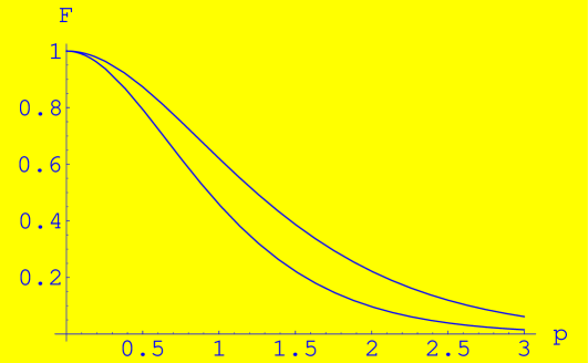
FIG. 3.: Form factor $F(p)$ for the $D^{*}D\pi$ strong coupling as a function of the pion momentum $p=|\vec{p}_{\pi}|$ in GeV. Normalization is for the soft pion limit. The two curves correspond to $<k>=400$ MeV (upper) and $<k>=300$ MeV (lower).

For $|\vec{p}_{\pi}|\simeq m_{B}/2$ we get therefore

$$F(|\vec{p}_{\pi}|)~{}=~{}0.065\pm 0.035~{},$$ (29)

where the central value corresponds to $<k>=350$ MeV and the higher (lower) to $<k>=400$ ($<k>=300$) MeV.

It should be observed that also the Lagrangean ${\cal L}_{HH\pi\pi}$ and the weak current $L^{\mu}$ have corrections from terms containing higher order derivatives. However these terms do not contribute to the imaginary part of $A_{LD}$; on the other hand hard pion and kaon effects in the calculation of to the real part can be taken into account by an appropriate cut-off of the Cottingham formula. We will discuss the problem in section 4.

III Imaginary part of the long-distance contribution

It can be easily seen that only diagrams 2c and 2d contribute to the discontinuity of $A_{LD}$. The diagrams 2a and 2b have no discontinuity, whereas the diagram 2e vanishes in the chiral limit and we neglect it altogether. As to the diagram 2f, both its imaginary and its real part vanish, as it can be easily checked.

We use the following kinematics:

$$p^{\mu}~{}=~{}m_{B}v^{\mu}=(m_{B},\vec{0})\ ,\ ~{}~{}~{}~{}p^{\mu}_{D^{(*)}}~{}=~{}m_{D}v^{\prime\mu}\ ,\ ~{}~{}~{}~{}q~{}=~{}p-p_{D^{(*)}}\ .$$ (30)

The discontinuity of the diagrams of figs. (2b, 2c) gives

$${\rm Disc}\ A_{LD} = 2\,i\,{\rm Im}\,A_{LD}=\,(-2\pi i)^{2}\int\frac{d^{4}q}{(2\pi)^{4}}\delta_{+}(q^{2}-m^{2}_{D_{s}})\,\delta_{+}(p^{2}_{D^{(*)}}-m^{2}_{D})\times$$ (31)

$$\times A(B\to D_{s}^{(*)}D^{(*)})\,A(D_{s}^{(*)}D^{(*)}\to K\pi)\ =$$ (33)

$$= \,-\frac{m_{D}}{16\pi^{2}m_{B}}\,{\sqrt{\omega^{*2}-1}}\,\int d\vec{n}\,A(B\to D_{s}^{(*)}D^{(*)})\,A(D_{s}^{(*)}D^{(*)}\to K\pi)\ ,$$ (35)

where $\displaystyle\omega^{*}\ =\ \frac{m_{B}^{2}+m_{D}^{2}-m^{2}_{D_{s}}}{2m_{D}m_{B}}$ and the angular integration is over the directions of the vector $\vec{v}^{\prime}=\vec{n}\sqrt{\omega^{{}^{*}2}-1}$. Our results are as follows:

$$A(B\to D_{s}D) = -\,K\,(m_{B}-m_{D})(1+\omega^{*})\ ,$$ (36)

$$A(B\to D_{s}^{*}(\eta,\,q)D^{*}(\epsilon,v^{\prime})) = K\,m_{D_{s}}\eta^{*\mu}\epsilon^{*\alpha}\left(i\epsilon_{\alpha\lambda\mu\sigma}v^{\prime\lambda}v^{\sigma}-g_{\mu\alpha}(1+\omega^{*})+v_{\alpha}v_{\mu}^{\prime}\right)\ ,$$ (38)

where $\displaystyle K\ =\ \frac{G_{F}}{\sqrt{2}}V_{cb}^{*}V_{cs}\ a_{2}\sqrt{m_{B}m_{D}}f_{D_{s}}\xi_{IW}(\omega^{*})\ .$ On the other hand we have

$$A(D_{s}D\to K\pi) = \ i\ \frac{\left(2g\,m_{D}\,F(|\vec{p}_{\pi}|)\right)^{2}}{f_{\pi}f_{K}}\ \times$$ (41)

$$\frac{-p_{\pi}\cdot p_{K}+p_{\pi}\cdot(q-p_{K})(p_{K}\cdot q-m^{2}_{K})/m^{2}_{D^{*}}}{(m_{D}v^{\prime}-p_{\pi})^{2}-m^{2}_{D^{*}}}\ ,$$

$$A(D_{s}^{*}(\eta,q)D^{*}(\epsilon,v^{\prime})\to K\pi) = \ i\ \frac{\left(2g\,F(|\vec{p}_{\pi}|)\right)^{2}{\sqrt{m_{D_{s}^{*}}m_{D^{*}}}}}{f_{\pi}f_{K}}\ \epsilon_{\lambda}\eta_{\sigma}\ \times$$ (45)

$$\left(\frac{m_{D^{*}}\ p_{\pi}^{\lambda}\,p_{K}^{\sigma}}{(m_{D^{*}}v^{\prime}-p_{\pi})^{2}-m^{2}_{D}}\ +\ \frac{G^{\sigma\lambda}(p_{\pi},p_{K},v^{\prime})}{(m_{D^{*}}v^{\prime}-p_{\pi})^{2}-m^{2}_{D^{*}}}\right),$$

where

$$G^{\sigma\lambda}(p_{\pi},p_{K},v^{\prime})= - (v^{\prime}\cdot q)\biggl{(}g^{\sigma\lambda}(p_{K}\cdot p_{\pi})-p_{\pi}^{\sigma}p_{K}^{\lambda}\biggr{)}\ -\ (q\cdot p_{\pi})\biggl{(}v^{\prime\sigma}p_{K}^{\lambda}-g^{\sigma\lambda}(v^{\prime}\cdot p_{K})\biggr{)}$$ (46)

$$- q^{\lambda}\biggl{(}p_{\pi}^{\sigma}(p_{K}\cdot v^{\prime})-v^{\sigma}(p_{K}\cdot p_{\pi})\biggr{)}\ .$$ (48)

We have not written down other amplitudes with no contribution to the discontinuity. Our numerical results obtained for the central value in Eq. (29) are reported in table 1.

TABLE I.: Numerical values for the imaginary part of $A_{LD}$. Units are GeV. First column refers to the $D,D_{s}$ intermediate state, the second column to the $D^{*},D^{*}_{s}$ intermediate state.

$D,\,D_{s}~{}$	$D^{*},\,D^{*}_{s}$	Total
$~{}1.45\times 10^{-8}~{}$	$0.89\times 10^{-8}$	$2.34\times 10^{-8}$

IV Real part of the long-distance contribution

The real part of the diagrams 2c and 2d could be computed by a dispersion relation, from their imaginary parts; however this procedure suffers from the uncertainty related to possible subtractions. A way to include them is to follow a Feynman diagram approach, using the Effective Lagrangean discussed in section 2. This basically amounts to including the real parts of figs. 2a and 2b and also the other diagrams of fig. 2 which, as we have seen, do not contribute to the imaginary part.

To compute $Re\ A_{LD}$ we first observe that we can change the integration variable in (13) from $q=p_{B}-p_{D^{(*)}}$ to the momentum $\ell$ defined by the formula

$$q=p_{B}-p_{D^{(*)}}\equiv(m_{B}-m_{D^{(*)}})v-\ell\ .$$ (49)

We note that, by this definition, $\ell$ measures the virtuality of the intermediate state while the velocities of the two hadrons coincide; one can always make this choice using the reparametrization invariance of the Heavy Quark Effective Theory [29]. The cut-off $\mu_{\ell}$ corresponding to the momentum $\ell$ can be evaluated, within our model, as follows. For an on-shell meson with momentum $p_{D}=m_{D}\,v$, the two constituent quarks have momenta $\vec{p}_{c}=\vec{k}$, $\vec{p}_{q}=-\vec{k}$ in the meson rest frame. Adding $\ell^{\mu}$ shifts $\vec{p}_{c}=\vec{k}\to\vec{k}+\vec{\ell}$; therefore the argument of the wave function appearing in the calculation of the Isgur-Wise function, instead of $|\vec{k}|$, is $|\vec{k}+\vec{\ell}/2|$. This corresponds to introducing in the amplitude the form factor $F(|\vec{\ell}|)$, with $F$ given in fig. 3. Moreover, we have to implement the condition that the residual momentum $\vec{k}+\vec{\ell}$ of the heavy quark does not exceed the chiral symmetry breaking scale, i.e. a mass scale around $1$ GeV. Since we assume $<k>=350$ MeV, this gives the condition $|\vec{\ell}|\leq 0.65$ GeV. The smooth form factor $F(|\vec{\ell}|)~{}(|\vec{\ell}|\leq 0.65~{}{\rm GeV})$ can be substituted by a sharp form factor $\theta(\mu_{\ell}-|\vec{\ell}|)$, and $\mu_{\ell}$ can be fixed by imposing $\displaystyle{\int_{0}^{0.65~{}{\rm GeV}}F(x)dx=\int_{0}^{\mu_{\ell}}dx}$. This procedure gives

$$\mu_{\ell}\approx 0.6~{}{\rm GeV}~{}.$$ (50)

On the other hand $\ell_{0}$ is of the order ${\vec{\ell}}^{\,2}/(2m_{c})$ and is therefore negligible in the large heavy quark mass limit. Therefore we conclude that a cut-off $\mu_{\ell}$ on $|\vec{\ell}|$ as given in (50) reflects in a cut-off $\mu^{2}_{\ell}$ on $\ell^{2}$. In passing, we observe that higher derivative corrections to the Lagrangean ${\cal L}_{HH\pi}+{\cal L}_{HH\pi\pi}$ and the weak current $L^{\mu}$ produce negligible effects due to this cut-off procedure.

Having fixed the cut-off we now compute the $\ell$ integration by performing a Wick rotation: $\ell^{0}\to i\ell^{0}$ and changing integration variable from $|\vec{\ell}|$ to $L^{2}~{}=~{}-((i\ell^{0})^{2}-\vec{\ell}^{2})$. We get therefore a Cottingham formula [23] as follows:

$${\rm Re}\ A_{LD}=\frac{i}{2\ (2\pi)^{3}}\frac{G_{F}}{\sqrt{2}}V_{cb}^{*}V_{cs}\ a_{2}\int_{0}^{\mu_{\ell}^{2}}dL^{2}\int_{-\sqrt{L^{2}}}^{+\sqrt{L^{2}}}dl_{0}\sqrt{L^{2}-l_{0}^{2}}\int_{-1}^{1}d\cos(\theta)\ i\left\{\frac{j_{D}^{\mu}\ h_{D\,\mu}}{p_{D}^{2}-m_{D}^{2}}+\frac{\sum_{pol}\ j_{D^{*}}^{\mu}\ h_{{D^{*}}\,\mu}}{p_{D^{*}}^{2}-m_{D^{*}}^{2}}\right\}.$$ (51)

Here $\displaystyle j_{D^{(*)}}^{\mu}=<D^{(*)}|\bar{b}\gamma^{\mu}(1-\gamma_{5})c|B>$, $\displaystyle h_{D^{(*)}}^{\mu}=<K\pi|\bar{c}\gamma^{\mu}(1-\gamma_{5})s|D^{(*)}>$. Both $j_{D^{(*)}}^{\mu}$ and $h_{D}^{\mu}$ can be found in [27]. The various contributions to the $h_{D^{*}}^{\mu}$, corresponding to the different graphs in fig. 2, are as follows:

$$h_{D^{*}\,\mu}^{(\ref{ff2}a)} = -i\ \frac{f_{D^{*}}m_{D^{*}}}{2\ f_{\pi}\ f_{K}}\varepsilon_{\mu}\;,$$ (52)

$$h_{D^{*}\,\mu}^{(\ref{ff2}b)} = i\ \frac{2\ \widetilde{g}f_{D^{*}}m_{D^{*}}}{f_{\pi}\ f_{K}}\frac{(\varepsilon\cdot p_{\pi})}{(p_{D^{*}}-p_{\pi})^{2}-m_{D}^{2}}(p_{D^{*}}-p_{\pi})_{\mu}+$$ (54)

$$\frac{2\ \widetilde{g}f_{D^{*}}m_{D^{*}}}{f_{\pi}\ f_{K}}\frac{1}{(p_{D^{*}}-p_{\pi})^{2}-m_{D^{*}}^{2}}\epsilon_{\mu\alpha\beta\gamma}\varepsilon^{\alpha}\ p_{\pi}^{\beta}\ p_{D^{*}}^{\gamma}\,\;,$$

$$h_{D^{*}\,\mu}^{(\ref{ff2}c)} = i\ \frac{4\ \widetilde{g}^{2}\ f_{D^{*}}m_{D^{*}}^{3}}{\ f_{\pi}\ f_{K}}\ \frac{(\varepsilon\cdot p_{\pi})}{[(p_{D^{*}}-p_{\pi})^{2}-m_{D}^{2}]\ [(p_{D^{*}}-p_{\pi}-p_{K})^{2}-m_{D^{*}_{s}}^{2}]}$$ (56)

$$\left[(p_{K})_{\mu}-\frac{(p_{D^{*}}\cdot p_{K})-(p_{\pi}\cdot p_{K})}{m_{D_{s}^{*}}^{2}}(p_{D^{*}}-p_{\pi}-p_{K})_{\mu}\right]\,\;,$$

$$h_{D^{*}\,\mu}^{(\ref{ff2}d)} = i\ \frac{4\ \widetilde{g}^{2}\ f_{D^{*}}m_{D^{*}}}{\ f_{\pi}\ f_{K}}\frac{1}{[(p_{D^{*}}-p_{\pi})^{2}-m_{D^{*}}^{2}]\ [(p_{D^{*}}-p_{\pi}-p_{K})^{2}-m_{D^{*}_{s}}^{2}]}$$ (60)

$$\biggl{\{}\biggl{[}(p_{D}^{*}\cdot p_{\pi})(\varepsilon\cdot p_{K})+(p_{\pi}\cdot p_{K})(\varepsilon\cdot p_{\pi})\biggr{]}\ (p_{D^{*}})_{\mu}+$$

$$\biggl{[}(p_{D^{*}}\cdot p_{\pi}-p_{D^{*}}^{2})(\varepsilon\cdot p_{K})-(p_{D^{*}}\cdot p_{K})(\varepsilon\cdot p_{\pi})\biggr{]}\ (p_{\pi})_{\mu}+$$

$$\biggl{[}(p_{D^{*}}^{2}-p_{D^{*}}\cdot p_{\pi})(p_{\pi}\cdot p_{K})-(p_{D^{*}}\cdot p_{K})(p_{D^{*}}\cdot p_{\pi})\biggr{]}\ \varepsilon_{\mu}\biggr{\}}\,\;,$$

$$h_{D^{*}\,\mu}^{(\ref{ff2}e)} = i\frac{f_{D^{*}}m_{D^{*}}}{\ f_{\pi}\ f_{K}}\ \frac{p_{D^{*}}\cdot(p_{\pi}-p_{K})}{(p_{D^{*}}-p_{\pi}-p_{K})^{2}-m_{D^{*}_{s}}^{2}}\left[\varepsilon_{\mu}+\frac{\varepsilon\cdot(p_{\pi}+p_{K})}{m_{D}^{2}}(p-p_{\pi}-p_{K})_{\mu}\right]\,\;,$$ (61)

$$h_{D^{*}\,\mu}^{(\ref{ff2}f)} = \frac{4\ \widetilde{g}^{2}f_{D^{*}}m_{D^{*}}}{\ f_{\pi}\ f_{K}}\ \frac{\epsilon_{\alpha\beta\gamma\delta}\ p_{\pi}^{\alpha}\ p_{D^{*}}^{\beta}\ p_{K}^{\gamma}\ \varepsilon^{\delta}}{[(p_{D^{*}}-p_{\pi})^{2}-m_{D^{*}}^{2}]\ [(p_{D^{*}}-p_{\pi}-p_{K})^{2}-m_{D^{*}_{s}}^{2}]}$$ (63)

$$(p_{D^{*}}-p_{\pi}-p_{K})_{\mu}\;\;,$$

where $\widetilde{g}=gF(|\vec{p}_{\pi}|)$. The results for $\mu_{\ell}\ =\ 0.5\div 0.7$ GeV are reported in table II.

All the terms in the previous equations containing the factor $g$ are corrected by the form factor $F(|\vec{p}_{\pi}|)$; the terms $h^{(2a)}$ and $h^{(2e)}$ should also contain their own multiplicative form factors $F_{a}$ and $F_{e}$ (this holds both for $D$ and $D^{*}$ intermediate states). We have not written down them explicitly for the following reasons. $F_{e}$ would multiply a term which vanishes in the chiral limit and does not affect the final result. On the other hand $F_{a}(q^{2})$ would represent a correction for hard pion and kaon momenta. In the region of high $q^{2}$, i.e. $q^{2}\in[m_{D}^{2},(m_{B}-m_{D})^{2}]$, $F_{a}(q^{2})$ is smooth and can be put equal to 1, i.e. to the value corresponding to the soft pion and kaon limit. This result can be inferred from the analogous behaviour of the form factor $F_{0}^{B\to\pi}(q^{2})$ describing the coupling of a heavy and one light meson. In the high $q^{2}$ region the contribution of the low lying pole $B(0^{+})$ to this form factor vanishes in the chiral limit and the form factor is dominated by the direct coupling displayed in Fig. 2a, giving, as a result, the simple formula $f_{B}/f_{\pi}$. Several numerical analyses confirm a smooth behaviour of $F_{0}^{B\to\pi}(q^{2})$. For example in the quark model of [33] $F_{0}^{B\to\pi}(q^{2})$ increases by $40\%$ in the range $15-26$ GeV²; this behaviour can be fitted by a formula

$$F_{0}^{B\to\pi}(q^{2})\propto\left(1-\frac{q^{2}}{(m_{B}+m_{\Lambda})^{2})}\right)^{-1}~{},$$ (64)

with $m_{\Lambda}\simeq 2.5$ GeV. In other models a smoother or similar behaviour is found, see the discussion in [33].

For $D$ decay this formula would hold with $m_{B}\to m_{D}$:

$$F_{0}^{D\to\pi}(q^{2})\propto\left(1-\frac{q^{2}}{(m_{D}+m_{\Lambda})^{2})}\right)^{-1}~{}.$$ (65)

However, it would be a too strong assumption to assume that $F_{a}(q^{2})$ is given by this formula; therefore we put $F_{a}=1$ in the sequel and we shall enlarge the theoretical uncertainty by an extra amount that we estimate $\pm 50\%$.

Let us finally observe that, while the numerical value of $F_{a}$ does not vary significantly in the range $q^{2}\in[m_{D}^{2},(m_{B}-m_{D})^{2}]$, its value for $q^{2}=(m_{B}-m_{D})^{2}$ is formally suppressed by one power of $(1/m_{b})$ as compared to $F_{a}(m_{D}^{2})$, assuming a qualitative behaviour analogous to $F_{0}^{D\to\pi}(q^{2})$.

TABLE II.: Numerical values for the real part of $A_{LD}$ for $\mu_{\ell}\ =\ 0.5\div 0.7$ GeV. First column refers to the $D$ intermediate state, the second column to the $D^{*}$ one. Units are GeV.

$\mu_{\ell}$	$D$	$D^{*}$	Total
$0.5$	$-4.66\times 10^{-9}$	$1.62\times 10^{-8}$	$1.15\times 10^{-8}$
$0.6$	$-7.77\times 10^{-9}$	$2.79\times 10^{-8}$	$2.01\times 10^{-8}$
$0.7$	$-1.19\times 10^{-8}$	$4.40\times 10^{-8}$	$3.21\times 10^{-8}$

V Conclusions

Our numerical results show that the long-distance charming penguin contributions to the decays $B\to K\pi$ are significant. These results agree qualitatively with a phenomenological analysis of these contributions given in [4]. In particular, we found that the absorptive part due to the $D,D_{s}$ states is somewhat bigger than that from the $D^{*},D_{s}^{*}$ states, but of the same sign. The real part due to the $D^{*},D_{s}^{*}$ states is however $3-4$ times bigger and opposite in sign to the contributions from the $D,D_{s}$ states. As shown in table 1 and table 2, the total contribution for the real part and absorptive part are of the same order of magnitude, at the $10^{-8}\rm\,GeV$ level. The results for the branching ratios are as follows:

$${\cal B}(B^{+}\to K^{0}\pi^{+}) = (2.4^{+2.7}_{-1.9})\times 10^{-5}$$ (66)

$${\cal B}(B^{0}\to K^{+}\pi^{-}) = (1.5^{+1.8}_{-1.3})\times 10^{-5}~{}.$$ (67)

The central values in this equation correspond to the central values of the parameters $g$, $<k>$ (i.e. $F{|\vec{p}_{\pi}|}$) and $\mu_{\ell}$. The theoretical uncertainties in the branching ratios are obtained by varying the parameters in the ranges $g=0.40\pm 0.08$, $<k>=(350\pm 50)$ GeV and $\mu_{\ell}=(0.6\pm 0.1)$ GeV. An extra theoretical uncertainty of $50\%$ has been added in quadrature to $ReA_{LD}$. The results in (67) agree with the experimental values in eq. (2).

The existence of two different contributions with different strong and weak phases produces a direct CP violation in the decay $B\to K^{\pm}\pi^{\mp}$. As a matter of fact, we find for

$${\cal A}=\frac{\Gamma(\bar{B}^{0}\to K^{-}\pi^{+})-\Gamma(B^{0}\to K^{+}\pi^{-})}{\Gamma(\bar{B}^{0}\to K^{-}\pi^{+})+\Gamma(B^{0}\to K^{+}\pi^{-})}$$ (68)

the value ${\cal A}=+0.21$ (for $\gamma=54.8^{0}$), which is compatible with the recent results from CLEO [34]. On the other hand the present model produces no CP asymmetries for charged $B$ decays into $K\pi$.

Let us finally discuss the problem of the scaling of our results with $m_{b}$. Assuming, as in [3], that $F_{0}^{B\to\pi}(0)$ scales as $\displaystyle\left(\frac{\Lambda_{QCD}}{m_{b}}\right)^{3/2}$, $A_{SD}$ scales as $m_{b}^{1/2}$. On the other hand the charming penguin contribution $A_{LD}$ is non leading due to the various form factors which vanish for $m_{b},\,m_{c}\to\infty$. Therefore the following conclusion can be drawn. The charming penguin contributions violate naive factorization and are of leading order in $\alpha_{s}$, as they arise from non perturbative calculations; nevertheless they do not contradict the results of [3, 35] since they are suppressed in the infinite heavy quark mass limits. In spite of that, as $m_{b},m_{c}$ in reality are finite, the charming penguin numerical contribution to the branching ratios in $B\to K\pi$ decays is significant, basically due to the enhancement of the CKM matrix elements.

In conclusion, we believe that the charmed resonance contributions we found seem to be capable of producing the charming-penguin terms suggested in [4] within theoretical errors. This method could then be applied also to other two-body nonleptonic $B$ decay channels, such as the $B\to\pi\pi$ and the $B\to K\eta^{\prime}$. We only mention here a result for the charming-penguin contribution in ${B}^{0}\to\pi^{+}\pi^{-}$ decay. This contribution can be obtained from the results we obtained for ${B}^{0}\to K^{+}\pi^{-}$ using $SU(3)$ symmetry for the weak current matrix elements $<K^{+}\pi^{-}|(\bar{c}s)_{L}|D_{s}>$ and $<\pi^{-}\pi^{+}|(\bar{c}d)_{L}|D^{-}>$. Thus, in the $SU(3)$ limit(by ignoring the $K-\pi$ mass difference) [27]

$$A_{\rm LD}({B}^{0}\to\pi^{+}\pi^{-})=(V_{cd}/V_{cs})(f_{K}/f_{\pi})\times A_{\rm LD}({B}^{0}\to K^{+}\pi^{-})~{}.$$ (69)

Since the ${B}^{0}\to\pi^{+}\pi^{-}$ decay is dominated by the tree-level operators, this charming-penguin contribution behaves like the penguin terms and reduces the ${B}^{0}\to\pi^{+}\pi^{-}$ decay rate by a small amount. The details of this work will be given elsewhere together with the results for $B\to K\eta^{\prime}$.

Acknowledgements We thank F. Ferroni for useful correspondence on the BaBar data.

REFERENCES

- [1] The BaBar Physics Book, edited by P. F. Harrison and H. R. Quinn, SLAC-R-504 (1998).
- [2] J. D. Bjorken, in New Developments in High-Energy Physics, Proc. IV International Workshop on High-Energy Physics, Orthodox Academy of Crete, Greece, 1–10 July 1988, edited by E. G. Floratos and A. Verganelakis, Nucl. Phys. B Proc. Suppl. 11 (1989) 325.
- [3] M. Beneke, G. Buchalla, M. Neubert and C. T. Sachrajda, Phys. Rev. Lett. 83 (1999) 1914; Nucl.Phys. B 591 (2000) 313; Contribution to ICHEP 2000, July 27 - August 2, Osaka, Japan, hep-ph/0007256.
- [4] M. Ciuchini, E. Franco, G. Martinelli and L. Silvestrini, Nucl. Phys. B 501 (1997) 271.
- [5] CLEO Collaboration, D.Cronin-Hennessy et al., Phys. Rev. Lett. 85 (2000) 515.
- [6] Talks presented by T.J. Champion (BaBar Collaboration) at the XXXth International Conference on High-Energy Physics, Osaka, Japan, 27 July – 2 August, 2000, SLAC-PUB-8696, BABAR-PROC-00/13, hep-ex/0011018.
- [7] Talks presented by P. Chang (Belle Collaboration) at the XXXth International Conference on High-Energy Physics, Osaka, Japan, 27 July – 2 August, 2000.
- [8] Talk presented by G. Cavoto (BaBar Collaboration) at XXXVI Rencontres de Moriond, 17–24 March, 2001, babar-talk-01/27.
- [9] Talk presented by B. Casey (Belle Collaboration) at XXXVI Rencontres de Moriond, 17–24 March, 2001, http://www.phys.hawaii.edu/casey/moriond.ps
- [10] J.-M. Gérard and W. S. Hou, Phys. Rev. Lett. 62 (1989) 855; Phys. Rev. D 43 (1991) 2909.
- [11] R. Fleischer, Z. Phys. C 58 (1993) 483; C 62 (1994) 81.
- [12] R. Fleischer and T. Mannel, Phys. Rev. D 57 (1998) 2752.
- [13] N. G. Deshpande and X. G. He, Phys. Lett. B 336 (1994) 471.
- [14] A. Ali, G. Kramer and Cai–Dian Lü, Phys. Rev. D 58 (1998) 094009.
- [15] A. Deandrea, N. Di Bartolomeo, F. Feruglio, R. Gatto and G. Nardulli Phys. Lett. B 320 (1993) 170.
- [16] N. G. Deshpande, X. G. He, W. S. Hou, and S. Pakvasa, Phys. Rev. Lett. 82 (1999) 2240.
- [17] C. Isola and T. N. Pham, Phys. Rev. D 62 (2000) 094002.
- [18] D. Du, D. Yang and G. Zhu, hep-ph/0005006.
- [19] T. Muta, A. Sugamoto, Mao–Zhi Yang and Ya–Dong Yang, Phys. Rev. D 62 (2000) 094020.
- [20] P. Colangelo, G. Nardulli, N. Paver and Riazuddin, Z.Phys. C 45 (1990) 575.
- [21] M. B. Voloshin and M. A. Shifman, Sov. J. Nucl. Phys. 45 (1987) 292; 47 (1988) 511.
- [22] D. Choudhury and J. Ellis, Phys. Lett. B 433 (1998) 102.
- [23] W. N. Cottingham, Ann. Phys. (N.Y.) 25 (1963) 424.
- [24] A. J. Buras, Probing the Standard Model of Particle Interactions, F. David and R. Gupta, eds, Elsevier Science B.V., hep-ph/9806471.
- [25] M. Ciuchini, E. Franco, G. Martinelli, L. Reina, and L. Silvestrini, Phys. Lett. B 316 (1993) 127; M. Ciuchini, E. Franco, G. Martinelli, and L. Reina, Nucl. Phys. B 415 (1994) 403.
- [26] M. Ciuchini et al., hep-ph/0012308.
- [27] C. L. Y. Lee, M. Lu and M. B. Wise, Phys. Rev. D 46 (1992) 5040.
- [28] B. Bajc, S. Fajfer and R. J. Oakes, Phys. Rev. D 53 (1996) 4957; B. Bajc, S. Fajfer, R. J. Oakes and S. Prelovsek, Phys. Rev. D 56 (1997) 7207; B. Bajc, S. Fajfer, R. J. Oakes and T. N. Pham, Phys. Rev. D 58 (1998) 054009.
- [29] R. Casalbuoni, A. Deandrea, N. Di Bartolomeo, F. Feruglio, R. Gatto and G. Nardulli, Phys. Rep. 281 (1997) 145.
- [30] P. Colangelo, F. De Fazio and G. Nardulli, Phys. Lett. B 334 (1994) 175.
- [31] P. Colangelo, F. De Fazio, M. Ladisa, G. Nardulli, P. Santorelli and A. Tricarico, Eur. Phys. J. C 8 (1999) 81.
- [32] M. Ladisa, G. Nardulli and P. Santorelli, Phys. Lett. B 455 (1999) 283.
- [33] A. Deandrea, R. Gatto, G. Nardulli, A.D. Polosa, Phys. Rev. D 61 (2000) 017502.
- [34] CLEO Collaboration, S. Chen et al., Phys. Rev. Lett. 85 (2000) 525.
- [35] Y. Y. Keum, H. N. Li and A. I. Sanda, hep-ph/0004004; hep-ph/0004173.