Radiative transitions in mesons in a non relativistic quark model

Abstract

In the framework of the non relativistic quark model, an exhaustive study of radiative transitions in mesons is performed. The emphasis is put on several points. Some traditional approximations (long wave length limit, non relativistic phase space, dipole approximation for E1 transitions, gaussian wave functions) are analyzed in detail and their effects commented. A complete treatment using three different types of realistic quark-antiquark potential is made. The overall agreement with experimental data is quite good, but some improvements are suggested.

1 Introduction

Quantum Chromodynamics (QCD) is today the only reliable theory for describing strong interactions. There exist many systems that can be used as a laboratory for exploring and testing the properties of this basic theory. Among them, the meson and baryon sectors have deserved a lot of investigations, essentially because they are very easily produced. However they belong to the non perturbative application of QCD and thus are not easy to be described from first principles. Despite many improvements in recent years, on both theoretical and computational sides, the lattice gauge calculations are still not completely reliable and cannot explain the whole bulk of known properties, even for the simplest systems such as the mesons, which consist of a valence quark-antiquark pair.

This explains why so many various phenomenological approaches have been developped in order to describe the non perturbative part of QCD. Among them the non relativistic quark model (NRQM) has met with an impressive number of successes [1]. The puzzling question is that it still works even in situations where it is expected to fail; there exist certainly some deep reasons for such a behaviour although they have not yet been clarified precisely (see [2]). Basically the NRQM needs to solve a Schrödinger type equation with two-body quark-quark (or quark-antiquark) interactions. In recent years, the determination of the interaction between constituent quarks has reached a high degree of sophistication and the whole spectra of mesons for instance can be accounted for in a rather satisfactory way [3].

However one does know that the description of the spectra is a necessary but not a sufficient condition for aiming at a good explanation of non perturbative QCD. In particular several very different potentials can give rise to spectra of the same quality. One needs other observables in order to test more precisely the resulting wave functions. A possibility is the study of static properties, such as magnetic moments or charged square radii. But more sensitive observables concern the transitions between various states or production mechanisms (which rely essentially on the same dynamical operators). One can think for instance on meson decays under strong forces (a resonance giving two or several mesons) or the decays under electroweak forces (a resonance producing a photon or leptons in the final channel). The advantage of this last kind of transition is that the transition operator is known perfectly well and thus it is easier to disantangle the drawbacks coming from less well known strong interactions through the meson wave function.

In fact this statement is not completely true in the NRQM. Being a phenomenological theory, NRQM deals with effective degrees of freedom, the constituent quarks, and a pure Dirac form of the quark-photon vertex in the transition operator is questionnable. Moreover, even in the traditional approach of radiative transitions (decay of a resonance into a resonance of lower energy plus a real photon) several types of approximations are of current use; the effect of these approximations can hide the necessity of using a more sophisticated vertex for the quark-photon coupling. Most of those approximations originate from the formulae widely used in atomic or nuclear physics which are simply translated in the meson sector. Let us mention the dipole approximation for E1 transitions, the long wave length approximation (LWLA) and a non relativistic phase space factor.

Although these approximations are fully justified in atomic or nuclear physics, it is not obvious that they continue to work when applied to mesons. Indeed in this sector the transition energy is typically $E_{\gamma}$ = $k_{\gamma}$ = 0.1–0.5 GeV, while the size of the source is roughly $R$ = 0.5–1 fm = 2.5–5 ${\rm GeV}^{-1}$, so that the long wave length condition $k_{\gamma}R<<1$ is not really justified. Comparing the photon energy to the mass of the emitting meson also convinces us that a non relativistic phase space is probably not suited. Moreover the fact that the electrons in an atom or the nucleons in a nucleus have the same mass is not true in the case of some mesons, and new phenomena can appear.

During the seventies and eighties, a lot of works has been done on radiative transitions for mesons (and also for baryons but we are not so interested in this sector here). At the very beginning they were studied in the vector dominance model [4, 5], then the quark model was introduced either in the framework of MIT bag model [6, 7, 8], the non relativistic quark model [9, 10, 11], 2 body Dirac equation [12, 13, 14] or some relativized phenemenological quark models [15, 16]. But even in the most complete and nice works, as [15] or [11], there is always an approximation or an inconsistency which plagues the results or forbids to draw precise conclusions. Most of relativistic models suffer of a bad treatment of the center of mass, relativized model do not treat with equal care the quark-quark potential and the electromagnetic operator. Moreover in many papers, a non relativistic phase space or a long wave length approximation are used and we will see that this is not justified in the meson sector. In addition, only very few studies concern the totality of the known experimental data but focus on very specific transitions (light quark sector or heavy quark sector or even more restricted sets).

The aim of this paper is essentially twofold. First, within a very precise framework namely the NRQM, we want to investigate deeply and with a particular care the effects of all these approximations as compared to an exact treatment. Second, we compare, on an exhaustive list of transitions and using an exact treatment, how different meson wave functions (obtained with different potentials giving meson spectra of similar quality) influence the results at the level of radiative transitions. We have in mind to see whether it is necessary to modify the quark-photon vertex; our study is thus a first necessary step before undertaking a more difficult and ambitious program.

In this paper we will consider all the radiative transitions (which are sufficiently reliable) that are reported in the particle data group booklet because we want an exhaustive analysis. The experimental data can be gathered into several groups :

• the transitions allowed by LWLA; they are essentially M1 transitions (${}^{3}S_{1}\rightarrow\>^{1}S_{0}$ or ${}^{1}S_{0}\rightarrow\>^{3}S_{1}$) and E1 transitions (${}^{3}P_{J}\rightarrow\>^{3}S_{1}$ or ${}^{3}S_{1}\rightarrow\>^{3}P_{J}$); there is also the particular E1 transition corresponding to the decay $b_{1}(1235)\rightarrow\pi\gamma$ ( ${}^{1}P_{1}\rightarrow\>^{1}S_{0}$)

• the transitions forbidden by LWLA; they are scarce but interesting : they correspond to ${}^{3}P_{J}\rightarrow\>^{1}S_{0}$, ${}^{3}S_{1}\rightarrow\>^{3}S_{1}$ and ${}^{1}P_{1}\rightarrow\>^{3}S_{1}$ transitions.

The paper is organized as follows. In the next section we present how the meson wave functions are obtained and also the different quark-antiquark potentials that we are studying. In the third chapter we recall the formalism necessary for the description of radiative transitions putting the emphasis on the general treatment and the differences corresponding to the various approximations that we want to discuss. In the fourth chapter our final expressions for the total widths are summarized. In the fifth chapter the results are presented and the effects of each approximation are analyzed in detail. Conclusions are relegated to the last chapter.

2 Description of mesons

In the NRQM, the meson is considered as a two particle system : a (constituent) quark of mass $m_{1}$ and an antiquark of mass $m_{2}$ submitted to a potential $V(r)$, so that the corresponding Schrödinger equation writes :

$$[m_{1}+m_{2}+\frac{{\bf p}^{2}}{2\mu}+V(r)]\mid\Psi_{\alpha}\rangle=m_{\alpha}\mid\Psi_{\alpha}\rangle$$ (1)

where $\mu$ is the reduced mass, ${\bf p}$ the relative momentum, and $m_{\alpha}$ the total mass of the resonance. This last quantity, as well as the wave function $\mid\Psi_{\alpha}\rangle$, of course depend on the choice for the potential. The ordinary quarks $u$ and $d$ can be considered as an isospin doublet; they are noted generically as $n$.

2.1 The potentials

In this paper we will consider three different types of potential, the so-called Bhaduri’s (BD) potential [17], AL1 and AP1 potentials [18]. For the purpose of our analysis, it is not necessary to introduce very sophisticated forms including spin-orbit, tensor forces, …whose effects are not so important and which complicate quite a lot the formalism. We limit ourselves to potentials containing two different structures : a central term and a hyperfine term; this is the minimum requirement to get reliable wave functions :

$$V(r)=V_{c}(r)+V_{h}(r){\bf\sigma_{1}}.{\bf\sigma_{2}}$$ (2)

In this expression, we forget about the color term which is always the same whatever the meson under consideration.

The central term $V_{c}(r)$ contains a short range coulomb part (remnant of one gluon exchange) and a confining term :

$$V_{c}(r)=-\frac{\kappa}{r}+ar^{p}-C$$ (3)

BD and AL1 potentials exhibit a traditional linear confinement ($p=1$) while AP1 potential uses $p=2/3$, a power best suited to Regge trajectories in non relativistic dynamics. In each potential the hyperfine term is short range (remnant of the Dirac factor of the Fermi-Breit approximation). For BD it is of Yukawa type:

$$V_{h}(r)=\frac{\kappa}{m_{1}m_{2}}\frac{exp(-r/r_{0})}{rr_{0}^{2}}$$ (4)

For AL1 and AP1 it is of gaussian type:

$$V_{h}(r)=\frac{2\kappa^{\prime}}{3m_{1}m_{2}}\frac{exp(-r^{2}/r_{0}^{2})}{\pi^{1/2}/r_{0}^{3}}$$ (5)

but, contrary to BD, the size is mass dependent through

$$r_{0}=A(2\mu)^{-B}$$ (6)

The parameters for the potentials are gathered in table (1). The meson spectra obtained with these potentials are rather good and have been presented elsewhere [18]. It is important to stress that they also give quite good results in the baryon sector; so we have some confidence that they describe the quark dynamics in a meson in a rather satisfactory way.

Table 1: Parameters for the three used potentials, defined by (2-6). All the units are in power of GeV.

BD AL1 AP1 $m_{u}=m_{d}=m_{n}$ 0.337 0.315 0.277 $m_{s}$ 0.600 0.577 0.553 $m_{c}$ 1.870 1.836 1.819 $m_{b}$ 5.259 5.227 5.206 $\kappa$ 0.520 0.5069 0.4242 $a$ 0.186 0.1653 0.3898 $p$ 1 1 2/3 $C$ 0.9135 0.8321 1.1313 $\kappa^{{}^{\prime}}$ - 1.8609 1.8025 $r_{0}$ 2.305 - - $A$ - 1.6553 1.5296 $B$ - 0.2204 0.3263

2.2 Meson wave functions

Because of the rotational invariance, the meson wave function is written as:

$$\mid\Psi_{ILSJ}\rangle=\eta_{I}(1,2)[\Phi_{nL}(1,2)\chi_{S}(1,2)]_{J}$$ (7)

where $\eta_{I}(1,2)$ is the isospin wave function with total isospin $I$, $\chi_{S}(1,2)$ is the spin wave function with total spin $S$ and $\Phi_{nL}(1,2)$ the space wave function with orbital momentum $L$ and radial number $n$. Spin $S$ and orbital momentum $L$ are coupled to total angular momentum $J$, but are nevertheless good quantum numbers. The color wave function is forgotten since it does not play any role in the formalism; the flavor content of the meson is also forgotten since the electromagnetic operator does not change the quark flavor. The magnetic quantum numbers are not indicated here although the projection of the isospin plays a role since the operator is a mixing of isoscalar and isovector terms. We will come back on this point later on.

We will use the expression of the space wave function both in position representation and in momentum representation. Thus we write :

$$\langle{\bf r}\mid\Phi_{nL}(1,2)\rangle = R_{nL}(r)Y_{L}(\hat{r})$$

$$\langle{\bf p}\mid\Phi_{nL}(1,2)\rangle = R_{nL}(p)Y_{L}(\hat{p})$$ (8)

We use the same notation for the radial wave function $R_{nL}$ in both representations if there is no risk of confusion. In fact the momentum representation is very often more convenient to deal with the matrix elements of the transition operator. Moreover an approximation of the exact wave function in terms of gaussian functions will be particularly well suited to compute easily difficult quantities. In this case we write:

$$R_{nL}(p)=p^{L}\sum_{i=1}^{N}c_{i}\exp(-A_{i}p^{2}/2)$$ (9)

and a similar expression for the wave function in coordinate representation. In general the number of gaussian terms needed in (9) to achieve convergence is rather weak. Just to give an idea of the quality of such an expansion in the case of AL1 potential, the masses $m_{\pi}$ and $m_{\rho}$ as function of $N$ are presented in Table (2) and compared to the exact ones (obtained by solving the differential equation with the Numerov algorithm). In the same spirit we plot the corresponding wave functions in figure (1). Although there is some differences between the $N$=1 and $N$=2 cases, one sees that very rapidly the approximation (9) can be identified to the exact solution. In practice we perform our calculations with $N$=5 and consider the corresponding wave function as the exact one. Let us also point out that, since the basis states are not orthogonal, different sets of ($c_{i},A_{i}$) parameters can be used with equal success. In fact, we determine these coefficients by two different methods : i) minimisation of the state with respect to these parameters, ii) best fit of the exact wave function with a form like (9). For $N$=5, both procedures give exactly the same results. Thus in the rest of the paper we qualify the wave function given by (9) with $N=5$ as the exact wave function.

Table 2: Convergence properties, with three different quark-antiquark potentials, for the $\pi$ and $\rho$ masses as function of the number of Gaussian functions NG in (9). This exact value is obtained with the Numerov algorithm.

BD AL1 AP1 $\pi$ 1G 0.252050 0.193702 0.192776 2G 0.157151 0.140359 0.140285 3G 0.141707 0.138436 0.138391 4G 0.138835 0.138220 0.138192 5G 0.138233 0.138188 0.138168 exact 0.138186 0.138057 0.138044 $\rho$ 1G 0.780344 0.771104 0.772196 2G 0.778425 0.770731 0.770166 3G 0.778402 0.770033 0.770156 4G 0.778375 0.770013 0.770036 5G 0.778374 0.770006 0.770029 exact 0.778347 0.769958 0.769988

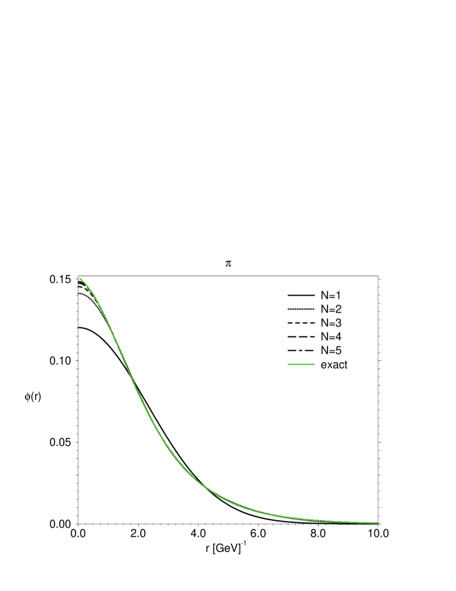
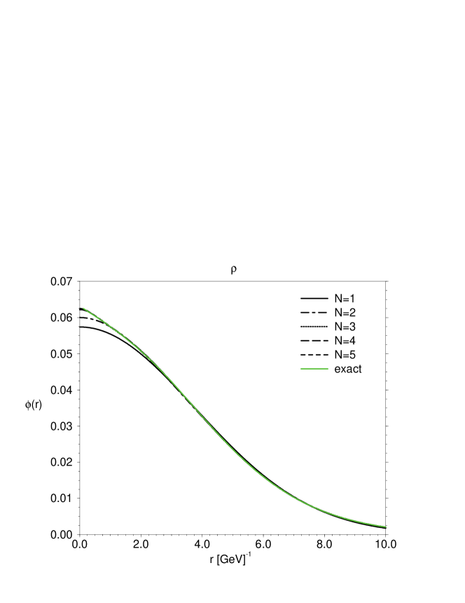
Figure 1: $\pi$ and $\rho$ radial wave functions $\frac{R_{nl}(r)}{\sqrt{4\pi}}$ for N=1 to 5 gaussian terms compared to the exact ones.

3 Radiative transitions

A number of points are already well known, and we do not want to spend too much time on them. We will focus our attention essentially on new aspects or on formulations that are discussed in details later on. Everywhere in this paper we employ natural units $\hbar=c=1$.

3.1 Transition operator

We start with the non relativistic expression of the electromagnetic transition operator between an initial meson state and a final meson state plus a real photon of momentum ${\bf k}$, energy E$=\mid{\bf k}\mid$ and polarisation ${\bf\epsilon}({\bf k},\lambda)$. We adopt, as usual, the Coulomb gauge, and we normalize the plane waves in a quantification volume $V$.

$$H_{I} = -\sqrt{\frac{2\pi\alpha}{VE}}{\bf\epsilon}({\bf k},\lambda)\cdot{\bf M}$$ (10)

$${\bf M} = \sum_{i=1}^{2}\frac{e_{i}}{2m_{i}}\ \exp(-i{\bf k}\cdot{\bf r}_{i})(2{\bf p}_{i}-i{\bf\sigma}_{i}\times{\bf k})$$ (11)

The summation runs on the two particles of charge $e_{i}$ and mass $m_{i}$ present in the meson. The first term in ${\bf M}$ is known as the electric term and the second one as the magnetic term.

3.2 Transition amplitude

The initial meson of mass $m_{a}$ is at rest and has angular momentum $J_{a}M_{a}$ (coupling of $L_{a}$ and $S_{a}$), isospin $I_{a}M_{I_{a}}$. The final meson of mass $m_{b}$ has a total momentum ${\bf K}_{b}$, angular momentum $J_{b}M_{b}$ (coupling of $L_{b}$ and $S_{b}$), isospin $I_{b}M_{I_{b}}$. Inserting ${\bf M}$ of (11) between the corresponding wave functions (in the rest frame of the meson ${\bf p}_{1}$ = - ${\bf p}_{2}$ = ${\bf p}$) in momentum representation (7) (completed by the center of mass plane wave), one gets the transition amplitude:

$${\bf M}_{A\rightarrow B}=\delta_{{\bf K}_{b},-{\bf k}}[{\bf M}^{(1)}_{A\rightarrow B}+{\bf M}^{(2)}_{A\rightarrow B}]$$ (12)

$${\bf M}^{(1)}_{A\rightarrow B} = \int d^{3}p\,\Phi^{*}_{B}({\bf p}-\frac{m_{2}}{m_{1}+m_{2}}{\bf k})[2{\bf p}-i{\bf\sigma}_{1}\times{\bf k}]\frac{<e_{1}>}{2m_{1}}\Phi_{A}({\bf p})$$ (13)

$${\bf M}^{(2)}_{A\rightarrow B} = \int d^{3}p\,\Phi^{*}_{B}({\bf p}+\frac{m_{1}}{m_{1}+m_{2}}{\bf k})[-2{\bf p}-i{\bf\sigma}_{2}\times{\bf k}]\frac{<e_{2}>}{2m_{2}}\Phi_{A}({\bf p})$$

where the subscripts refer to the particle number, see figure (2).

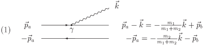
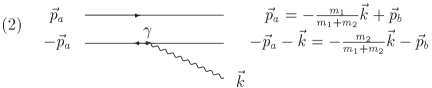
Figure 2: Schematic representation of the elementary decay process with momentum values from the rest frame of the inital meson. (1) denotes the emission of the real photon by the quark and gives rise to $M^{(1)}$ and (2) by the antiquark and gives rise to $M^{(2)}$.

We must say a word about the charge and its relation to isospin. One can perfectly well ignore isospin degrees of freedom and speak only of flavor wave function and its symmetry properties. In this case $e_{i}$ is simply a physical quantity, the charge corresponding to the flavor of quark i; we understand $<e_{i}>$ appearing in (13) as $e_{i}$. On the other hand, one can also introduce isospin degrees of freedom for convenience, in particular, it makes things easier in the case of neutral mesons with flavor mixing or mixing angles; for isospin $t_{i}$=0 one still has $<e_{i}>$ = $e_{i}$. However for isospin $t_{i}$=1/2, the charge is different for each member of the multiplet so that it becomes an isospin dependent operator $e_{i}=\pm 1/6+(t_{i})_{z}$ (+ for quark, - for antiquark). In this case on must understand $<e_{i}>$ as the matrix element of this operator on isospin wave function $\eta_{I}$. If we adopt this philosophy, a very simple calculus, based on Racah algebra, gives :

t2IaIb}]t1=1/2\displaystyle\left.<I_{a}M_{I_{a}}10\mid I_{b}M_{I_{b}}>\left\{\begin{tabular}[]{ccc}1&1/2&1/2\\ $t_{2}$&$I_{a}$&$I_{b}$\\ \end{tabular}\right\}\right]\,\hskip 14.22636ptt_{1}=1/2 t1IaIb}]t2=1/2\displaystyle\left.<I_{a}M_{I_{a}}10\mid I_{b}M_{I_{b}}>\left\{\begin{tabular}[]{ccc}1&1/2&1/2\\ $t_{1}$&$I_{a}$&$I_{b}$\\ \end{tabular}\right\}\right]\,\hskip 14.22636ptt_{2}=1/2

$$<e_{i}> = e_{i}\,\delta_{I_{a}I_{b}}\,\delta_{M_{I_{a}}M_{I_{b}}}\,\hskip 42.67912ptt_{i}=0$$

$$<e_{1}> = \delta_{M_{I_{a}}M_{I_{b}}}\left[\frac{1}{6}\delta_{I_{a}I_{b}}+(-1)^{I_{a}+t_{2}-1/2}\sqrt{3(I_{a}+1/2)}\right.$$ (16)

11/21/2

$$<e_{2}> = \delta_{M_{I_{a}}M_{I_{b}}}\left[-\frac{1}{6}\delta_{I_{a}I_{b}}+(-1)^{I_{b}+t_{1}-1/2}\sqrt{3(I_{a}+1/2)}\right.$$ (19)

11/21/2

3.2.1 Long Wave Length Approximation

Due to the recoil term in meson $B$ wave function, the space term appearing in (13) is not easy to calculate. A widely used approximation is the long wave length approximation (LWLA) which consists in putting ${\bf k}$=0 in the argument of $\Phi_{B}$ (this is equivalent to replace $\exp(-i{\bf k}\cdot{\bf r})$ by 1 in coordinate representation). It is just a matter of Racah algebra to disantangle the spin and space degrees of freedom in (13). It is pleasant that, in this case, the electric and magnetic part, which are of different parity, cannot couple the same states; this is why we speak about electric and magnetic transitions. It is also convenient to calculate the covariant spherical components $\mu=-1,0,1$ of the vector ${\bf M}$.

The electric transitions change the parity of the state, but not the spin. One has, for the $\mu$ component :

$$({\bf M}^{e}_{A\rightarrow B})_{\mu}=\delta_{S_{a},S_{b}}\delta_{{\bf K}_{b},-{\bf k}}<J_{a}M_{a}1\mu\mid J_{b}M_{b}>F^{e}(A\rightarrow B)$$ (20)

with the expression $F^{e}$, independent of the magnetic numbers:

$$F^{e}(A\rightarrow B) = (-1)^{S_{a}+J_{a}+L_{b}+1}(\frac{<e_{1}>}{m_{1}}-\frac{<e_{2}>}{m_{2}})\hat{L_{a}}\hat{J_{a}}<L_{a}010\mid L_{b}0>$$ (23)

$$\left\{\begin{tabular}[]{ccc}$L_{a}$&$S_{a}$&$J_{a}$\\ $J_{b}$&1&$L_{b}$\\ \end{tabular}\right\}\int_{0}^{\infty}dp\,R_{n_{b}L_{b}}(p)R_{n_{a}L_{a}}(p)p^{3}$$

where we have introduced the usual notation $\hat{J}$=$\sqrt{2J+1}$.

The magnetic transitions do not change parity nor orbital momentum. Since the operator contains a spin dependent part, the decoupling is a little bit more complicated but straightforward anyhow:

$$({\bf M}^{m}_{A\rightarrow B})_{\mu} = \delta_{L_{a},L_{b}}\delta_{{\bf K}_{b},-{\bf k}}F^{m}(A\rightarrow B)$$ (24)

$$\sum_{\nu,\sigma}<1\nu 1\sigma\mid 1\mu><J_{a}M_{a}1\nu\mid J_{b}M_{b}>k_{\sigma}$$

with the expression $F^{m}$, independent of the magnetic numbers:

1/2SaSb}fragmentsS𝑎fragmentsL𝑎fragmentsJ𝑎fragmentsJ𝑏1fragmentsS𝑏fragments 1/2fragmentsS𝑎fragmentsS𝑏\displaystyle\left\{\begin{tabular}[]{ccc}$S_{a}$&$L_{a}$&$J_{a}$\\ $J_{b}$&1&$S_{b}$\\ \end{tabular}\right\}\left\{\begin{tabular}[]{ccc}1&1/2&1/2\\ 1/2&$S_{a}$&$S_{b}$\\ \end{tabular}\right\}

$$F^{m}(A\rightarrow B) = (-1)^{L_{a}+J_{b}}\sqrt{3}(\frac{<e_{1}>}{m_{1}}+(-1)^{S_{a}+S_{b}}\frac{<e_{2}>}{m_{2}})\hat{S_{a}}\hat{J_{a}}\hat{S_{b}}$$

11/21/211/21/2

$$\int_{0}^{\infty}dp\,R_{n_{b}L_{b}}(p)R_{n_{a}L_{a}}(p)p^{2}$$

Of course, when the gaussian expansion of the wave function (9) is employed, the dynamical integrals are analytical.

3.2.2 Beyond long wave length approximation

The big advantage of using the wave functions expressed on gaussian terms (9) is that the treatment of the general case can be dealt with rather simply. Since taking $N$=5 is equivalent to treat the exact wave function, the following treatment solves exactly the problem. In fact an individual term in the expansion is of the form $\Phi_{L}({\bf p})=\exp(-Ap^{2}/2)\mathcal{Y}_{L}({\bf p})$ where $\mathcal{Y}_{L}({\bf p})=p^{L}Y_{L}(\hat{p})$ is the usual solid harmonic. Just to illustrate the procedure, let us consider only one term in the expansion (one $A$ quantity for meson A, one $B$ quantity for meson B) with a unit amplitude $c^{A}=c^{B}=1$). The argument in meson B wave function is now a linear combination of ${\bf p}$ and ${\bf k}$. Such a combination in the solid harmonic can be treated using the formulae :

$$\mathcal{Y}_{lm}(a{\bf p}_{1}+b{\bf p}_{2}) = \sum_{l_{1}=0}^{l}C_{l_{1}}^{l}a^{l_{1}}b^{l-l_{1}}[\mathcal{Y}_{l_{1}}({\bf p}_{1})\mathcal{Y}_{l-l_{1}}({\bf p}_{2})]_{lm}$$

$$C_{l_{1}}^{l} = \sqrt{\frac{4\pi(2l+1)!}{(2l_{1}+1)!(2(l-l_{1})+1)!}}$$ (30)

and

000)superscript1𝑙^subscript𝑙1^subscript𝑙24𝜋fragments 000\displaystyle(-1)^{l}\frac{\hat{l_{1}}\hat{l_{2}}}{\sqrt{4\pi}}\left(\begin{tabular}[]{ccc}$l_{1}$&$l_{2}$&l\\ 0&0&0\end{tabular}\right)

$$[\mathcal{Y}_{l_{1}}({\bf p})\mathcal{Y}_{l_{2}}({\bf p})]_{lm} = B_{l_{1}l_{2}}^{l}p^{l_{1}+l_{2}-l}\mathcal{Y}_{lm}({\bf p})$$

$$B_{l_{1}l_{2}}^{l} = (-1)^{l}\frac{\hat{l_{1}}\hat{l_{2}}}{\sqrt{4\pi}}\left(\begin{tabular}[]{ccc}$l_{1}$&$l_{2}$&l\\ 0&0&0\end{tabular}\right)$$ l1l2ll1l2l (33)

The same combination appearing in the exponential is a quadratic form which can be diagonalized in order to get rid of the non diagonal terms. Let us just summarize our conclusions.

Here are some auxilliary quantities ($i=1,2$ refers to particle number):

$$D=\frac{A+B}{2}\;;\;x^{(i)}=\frac{m_{3-i}B}{(m_{1}+m_{2})(A+B)}$$ (34)

$$z^{(i)}=\frac{m_{3-i}A}{(m_{1}+m_{2})(A+B)}\;;\;F^{(i)}=Dx^{(i)}z^{(i)}$$

If the masses of the quark and the antiquark are the same there is no need to distinguish the quantities $x,z,F$ and further simplifications arise which we do not want to comment. The transition amplitudes in the general case can be converted to a more appropriate form:

$${\bf M}^{(1)}_{A\rightarrow B} = \frac{<e_{1}>}{2m_{1}}\int d^{3}q\exp(-Dq^{2}-F^{(1)}k^{2})[\mathcal{Y}^{*}_{L_{b}}({\bf q}-z^{(1)}{\bf k})\chi_{S_{b}}]_{J_{b}}$$

$$[2{\bf q}-i{\bf\sigma}_{1}\times{\bf k}][\mathcal{Y}_{L_{a}}({\bf q}+x^{(1)}{\bf k})\chi_{S_{a}}]_{J_{a}}$$

$${\bf M}^{(2)}_{A\rightarrow B} = \frac{<e_{2}>}{2m_{2}}\int d^{3}q\exp(-Dq^{2}-F^{(2)}k^{2})[\mathcal{Y}^{*}_{L_{b}}({\bf q}+z^{(2)}{\bf k})\chi_{S_{b}}]_{J_{b}}$$ (35)

$$[-2{\bf q}-i{\bf\sigma}_{2}\times{\bf k}][\mathcal{Y}_{L_{a}}({\bf q}-x^{(2)}{\bf k})\chi_{S_{a}}]_{J_{a}}$$

Altough it is possible to pursue the calculations using (3.2.2), experimentally all the known transitions exhibit either $L_{a}$=0 or $L_{b}$=0. The resulting formulae look much more sympathetic in those cases and we report here only these special cases since only them will be applied in the next chapter. One important difference, as compared to the LWLA, is that both the electric and magnetic terms of the operator contributes to a given transition. Let us present the result for $L_{b}=0$.

$$({\bf M}_{A\rightarrow BL_{b}=0})_{\mu}=\delta_{S_{b},J_{b}}[\mathcal{E}_{\mu}(A;x)+\mathcal{M}_{\mu}(A;x)]$$ (36)

The term $\mathcal{E}_{\mu}(A;x)$ comes from the electric part of the operator and writes:

$$\mathcal{E}_{\mu}(A;x)=\delta_{S_{a},S_{b}}\frac{\sqrt{4\pi L_{a}}}{6}\hat{L_{a}}\Gamma(5/2)<L_{a},M_{a}-M_{b};J_{b},M_{b}\mid J_{a},M_{a}>$$ (37)

$$<1,-\mu;L_{a}-1,M_{a}-M_{b}+\mu\mid L_{a},M_{a}-M_{b}>(-1)^{\mu}\mathcal{Y}_{L_{a}-1,M_{a}-M_{b}+\mu}({\bf k})$$

$$\left[\frac{<e_{1}>}{m_{1}}\frac{(x^{(1)})^{L_{a}-1}\exp(-F^{(1)}k^{2})}{D^{5/2}}+(-1)^{L_{a}}\frac{<e_{2}>}{m_{2}}\frac{(x^{(2)})^{L_{a}-1}\exp(-F^{(2)}k^{2})}{D^{5/2}}\right]$$

Note that this term vanishes if $L_{a}=0$.

The term $\mathcal{M}_{\mu}(A;x)$ comes from the magnetic part of the operator and writes:

1/2SaJb}subscriptℳ𝜇𝐴𝑥superscript11subscript𝑆𝑎2𝜋Γ32^subscript𝑆𝑎fragments 1/2fragmentsS𝑎fragmentsJ𝑏\mathcal{M}_{\mu}(A;x)=(-1)^{1+S_{a}}2\pi\Gamma(3/2)\hat{S_{a}}\left\{\begin{tabular}[]{ccc}1&1/2&1/2\\ 1/2&$S_{a}$&$J_{b}$\\ \end{tabular}\right\}

11/21/211/21/2 (38)

$$\left[\frac{<e_{1}>}{m_{1}}\frac{x^{(1)\ L_{a}}\exp(-F^{(1)}k^{2})}{D^{3/2}}+(-1)^{L_{a}+S_{a}+J_{b}}\frac{<e_{2}>}{m_{2}}\frac{x^{(2)\ L_{a}}\exp(-F^{(2)}k^{2})}{D^{3/2}}\right]$$

$$\sum_{\mu_{a},\sigma_{a},\nu,\sigma}<L_{a}\mu_{a}S_{a}\sigma_{a}\mid J_{a}M_{a}><S_{a}\sigma_{a}1\nu\mid J_{b}M_{b}><1\nu 1\sigma\mid 1\mu>\mathcal{Y}_{1\sigma}({\bf k})\mathcal{Y}_{L_{a}\mu_{a}}({\bf k})$$

The case $L_{a}=0$ looks very similar, but one has to be very careful with the phases. In this case the electric part is given by

$$\mathcal{E}_{\mu}(B;z)=(-1)^{L_{b}-1-\mu}\mathcal{E}^{*}_{-\mu}(A=B;x=z)$$ (39)

meaning that in expression (37), one has to change all quantities relative to A by the corresponding ones relative to B, change the sign of $\mu$, change $x$ by $z$, take the complex conjugate and multiply by a given phase. The expression for $\mathcal{M}_{\mu}(B;z)$ is obtained with the same prescription as (39).

If one admits more than one gaussian function in the expansion of the wave function the quantities defined in (34) depends on which terms are retained and must be written more explicitly i.e $D_{ij}$ = $(A_{i}+B_{j})/2$. To obtain the complete expression corresponding to the exact wave function, one must take care of this; for example one must make in (37-38) the following replacement:

$$\frac{(x^{(1)})^{L_{a}-1}\exp(-F^{(1)}k^{2})}{D^{5/2}}\rightarrow\sum_{i,j=1}^{N}c_{i}^{A}c_{j}^{B}\frac{(x_{ij}^{(1)})^{L_{a}-1}\exp(-F_{ij}^{(1)}k^{2})}{D_{ij}^{5/2}}$$ (40)

and similar replacements everywhere.

4 The phase space

4.1 density of states

The density of states is obtained with periodic conditions in the quantification box. The treatment can be found in any textbook. The density of states by energy unit and by solid angle unit is given by

$$\rho(E,\Omega)=\frac{VE^{2}}{(2\pi)^{3}}$$ (41)

One has to calculate the matrix element $<B\gamma|H_{i}|A>^{2}$ from (10). The best way is to use spherical components for the vectors and Racah algebra to deal with the corresponding expressions. One has then to sum over the polarisations of the photon and of the final meson and to average over the polarisations of the decaying meson. In order to simplify the notations, let us introduce the quantity $X(E)$ by:

$$X(E)\delta_{\vec{K}_{b},-\vec{k}}=\frac{1}{\hat{J_{A}}^{2}}\sum_{\lambda=\pm 1}\sum_{M_{a},M_{b}}\mid<B\gamma|H_{i}|A>\mid^{2}$$ (42)

The decay width is given by the golden rule:

$$\Gamma=\int dE\ \delta(E_{f}-E_{i})\int d\Omega\ 2\pi\ \rho(E,\Omega)X(E)$$ (43)

In the litterature, one finds different formulae for the width depending upon how is treated the energy Dirac term in (43). This is known as the phase space factor $\Phi$. Explicitly, one writes :

$$\Gamma=\Phi(E_{0})VX(E_{0})$$ (44)

As this must be, the quantification volume $V$, appearing in (44), cancels with the one present in $X(E)$ as seen in (10). $E_{0}$ denotes the energy value fulfilling the equation $E_{f}=E_{i}$.

4.2 relativistic phase space

In this case the energies $E_{f}$ and $E_{i}$ are given by their relativistic expressions. Taking into account the fact that the momentum of the final meson is opposite to the photon momentum, the Dirac factor is $\delta(E_{B}+E-m_{a})=\delta(\sqrt{m_{b}^{2}+E^{2}}+E-m_{a})$. The integral in (43) is performed with the usual rules on delta functions to give :

$$\Phi(E_{0})=\frac{E_{0}^{2}}{\pi}\frac{E_{B}(E_{0})}{m_{a}}\;;\;E_{0}=\frac{m_{a}^{2}-m_{b}^{2}}{2m_{a}}$$ (45)

4.3 Non relativistic phase space

In a non relativistic treatment, the energies are related to their momenta by the classical expressions. Alternatively, one can make the approximation $E_{0}<<m_{a},\ m_{b}$ in the relativistic phase (45).

$$\Phi(E_{0})=\frac{E_{0}^{2}}{\pi}\;;\;E_{0}=m_{a}-m_{b}$$ (46)

Thus, as compared to the relativistic expression, the non relativistic phase space differs by two effects. The energy of the photon is equal to the energy difference between the resonances (as in nuclear physics) and the term $\frac{E_{B}(E_{0})}{m_{a}}$ is equal to unity.

4.4 mixed phase space

The mixed phase space is sometimes used in litterature [13]. It consists in retaining the relativistic value (45) for the energy $E_{0}$ – because the effect should be important in the meson sector – but the non relativistic value (46) for $\Phi(E_{0})$. Thus the mixed phase space is based on :

$$\Phi(E_{0})=\frac{E_{0}^{2}}{\pi}\;;\;E_{0}=\frac{m_{a}^{2}-m_{b}^{2}}{2m_{a}}$$ (47)

5 Total widths

5.1 long wave length approximation

With expression (20) for the amplitude and (44) and (45) for the phase space, the total width for electric transition is obtained after some calculations:

$$\Gamma^{e}_{A\rightarrow B\gamma} = \delta_{S_{a},S_{b}}4\frac{\alpha}{3}E_{0}\frac{E_{B}(E_{0})}{m_{a}}(\frac{<e_{1}>}{m_{1}}-\frac{<e_{2}>}{m_{2}})^{2}$$ (51)

$$\hat{L_{a}}^{2}\hat{J_{b}}^{2}<L_{a}010\mid L_{b}0>^{2}\left\{\begin{tabular}[]{ccc}$L_{a}$&$S_{a}$&$J_{a}$\\ $J_{b}$&1&$L_{b}$\\ \end{tabular}\right\}^{2}$$

$$\left[\int_{0}^{\infty}dp\,R_{n_{b}L_{b}}(p)R_{n_{a}L_{a}}(p)p^{3}\right]^{2}$$

In the same way the magnetic transition width results from the expression (24) for the amplitude. It looks like :

1/2SaSb}2​{SaLaJaJb1Sb}2superscript^subscript𝑆𝑎2superscript^subscript𝑆𝑏2superscript^subscript𝐽𝑏2superscriptfragments 1/2fragmentsS𝑎fragmentsS𝑏2superscriptfragmentsS𝑎fragmentsL𝑎fragmentsJ𝑎fragmentsJ𝑏1fragmentsS𝑏2\displaystyle\hat{S_{a}}^{2}\hat{S_{b}}^{2}\hat{J_{b}}^{2}\left\{\begin{tabular}[]{ccc}1&1/2&1/2\\ 1/2&$S_{a}$&$S_{b}$\\ \end{tabular}\right\}^{2}\left\{\begin{tabular}[]{ccc}$S_{a}$&$L_{a}$&$J_{a}$\\ $J_{b}$&1&$S_{b}$\\ \end{tabular}\right\}^{2}

$$\Gamma^{m}_{A\rightarrow B\gamma} = \delta_{L_{a},L_{b}}2\alpha E_{0}^{3}\frac{E_{B}(E_{0})}{m_{a}}(\frac{<e_{1}>}{m_{1}}+(-1)^{S_{a}+S_{b}}\frac{<e_{2}>}{m_{2}})^{2}$$ (57)

11/21/211/21/2

$$\left[\int_{0}^{\infty}dp\,R_{n_{b}L_{b}}(p)R_{n_{a}L_{a}}(p)p^{2}\right]^{2}$$

These formulae hold for a relativistic phase space. The modification due to the use of a non relativistic or a mixed phase space results obviously from the discussion of the previous chapter. Simplified expressions applied to specific transitions seen experimentally are relegated to the appendix.
Very often, the electric transition is calculated using the dipole approximation. The advantage is that it is not necessary to have the meson wave function in momentum representation but in coordinate representation which is a more natural scheme, while avoiding a complicated nabla operator. However one must be very careful in handling it because it relies on some approximations which are not always justified. Indeed the dynamical factor appearing in the amplitude is proportionnal to : $\langle B\mid{\bf p}\mid A\rangle$. The widely used trick is to remark that ${\bf p}$ is itself proportionnal to $\left[\ H_{int},\ {\bf r}\ \right]$ so that $\langle B\mid{\bf p}\mid A\rangle\ =i\mu(m_{a}-m_{b})\langle B\mid{\bf r}\mid A\rangle$, where $\mu$ is the reduced mass of the meson system (this is sometimes known as the Siegert theorem).

Thus the only change to the previous derivation of the decay width for the eletric term in equation (51) is the replacement of $\int_{0}^{\infty}dp\,R_{n_{b}L_{b}}(p)R_{n_{a}L_{a}}(p)p^{3}$ by $\mu(m_{a}-m_{b})\int_{0}^{\infty}dr\,R_{n_{b}L_{b}}(r)R_{n_{a}L_{a}}(r)r^{3}$. But, in so doing, one must be sure of two things : i) the quark-antiquark potential does not depend on velocity (this is the case in our calculations) ii) the meson wave functions are the true eigenstates of $H_{int}$. Even in this case $(m_{a}-m_{b})$ is the calculated value with a given potential and not the experimental value.

Moreover, we find also a very popular additional approximation which consists in the replacement of $E_{0}(m_{a}-m_{b})^{2}$ appearing in the width by $E_{0}^{3}$. This is acceptable in a non relativistic situation but not in a relativistic one. All these approximations are of course the remnants of the theory applied in atomic or nuclear physics. We also discuss this point in the next section.

In the rest of the text this approximation will be called the dipole approximation (DA).

5.2 general case

We now come to the expression of the width in the general case, but with the wave functions expanded on gaussian terms, as discussed in details previously. We present the results only in the case $L_{b}=0$. The results for $L_{a}=0$ are easily obtained from these ones with the correct replacement (39) and the modification due to spin average. We do not want to enter into too much details because the calculations are essentially a tricky application of Racah algebra. We report the result below :

$$\Gamma_{A\rightarrow B\gamma}=\delta_{S_{b},J_{b}}2\alpha\frac{E_{B}(E_{0})}{m_{a}}[\mathcal{EE}+\mathcal{EM}+\mathcal{MM}]$$ (58)

The terms $\mathcal{EE},\mathcal{EM},\mathcal{MM}$ come from the electric-electric, electric- magnetic, magnetic-magnetic part in the square of the amplitude. One sees that a transition is no longer of purely electric or magnetic type, but a mixing of both with interference effects. They are given by :

1/2SaJb}​{LaSaJaJbLa1}​k02​La+1​𝒜​ℬfragments 1/2fragmentsS𝑎fragmentsJ𝑏fragmentsL𝑎fragmentsS𝑎fragmentsJ𝑎fragmentsJ𝑏fragmentsL𝑎1superscriptsubscript𝑘02subscript𝐿𝑎1𝒜ℬ\displaystyle\left\{\begin{tabular}[]{ccc}1&1/2&1/2\\ 1/2&$S_{a}$&$J_{b}$\\ \end{tabular}\right\}\left\{\begin{tabular}[]{ccc}$L_{a}$&$S_{a}$&$J_{a}$\\ $J_{b}$&$L_{a}$&1\\ \end{tabular}\right\}k_{0}^{2L_{a}+1}\mathcal{A}\mathcal{B} 1/2SaJb}2​k02​La+3​ℬ234Γsuperscript322superscript^subscript𝑆𝑎2superscript^subscript𝐿𝑎2superscript^subscript𝐽𝑏2superscriptfragments 1/2fragmentsS𝑎fragmentsJ𝑏2superscriptsubscript𝑘02subscript𝐿𝑎3superscriptℬ2\displaystyle\frac{3}{4}\Gamma(3/2)^{2}\hat{S_{a}}^{2}\hat{L_{a}}^{2}\hat{J_{b}}^{2}\left\{\begin{tabular}[]{ccc}1&1/2&1/2\\ 1/2&$S_{a}$&$J_{b}$\\ \end{tabular}\right\}^{2}k_{0}^{2L_{a}+3}\mathcal{B}^{2}

$$\mathcal{EE} = \delta_{S_{a},S_{b}}\frac{\Gamma(5/2)^{2}}{36}L_{a}(L_{a}+1)k_{0}^{2L_{a}-1}\mathcal{A}^{2}$$

$$\mathcal{EM} = \delta_{S_{a},S_{b}}(-1)^{L_{a}+S_{a}+J_{a}+J_{b}+1}\frac{\Gamma(3/2)\Gamma(5/2)}{2\sqrt{6}}\sqrt{L_{a}(L_{a}+1)}\hat{S_{a}}\hat{L_{a}}\hat{J_{b}}$$ (63)

11/21/211/21/2

$$\mathcal{MM} = \frac{3}{4}\Gamma(3/2)^{2}\hat{S_{a}}^{2}\hat{L_{a}}^{2}\hat{J_{b}}^{2}\left\{\begin{tabular}[]{ccc}1&1/2&1/2\\ 1/2&$S_{a}$&$J_{b}$\\ \end{tabular}\right\}^{2}k_{0}^{2L_{a}+3}\mathcal{B}^{2}$$ 11/21/211/21/2 (69)

$$\sum_{J}<1\;1\;L_{a}\;0\mid J\;1>^{2}\left\{\begin{tabular}[]{ccc}$L_{a}$&$S_{a}$&$J_{a}$\\ $J_{b}$&$J$&1\\ \end{tabular}\right\}^{2}$$

where the dynamical factors $\mathcal{A}$ and $\mathcal{B}$ result from the meson wave functions :

$$\mathcal{A} = \frac{<e_{1}>}{m_{1}}\sum_{i,j}\frac{c_{i}^{A}c_{j}^{B}(x_{ij}^{(1)})^{L_{a}-1}\exp(-F_{ij}^{(1)}k_{0}^{2})}{D_{ij}^{5/2}}$$ (70)

$$+ (-1)^{L_{a}}\frac{<e_{2}>}{m_{2}}\sum_{i,j}\frac{c_{i}^{A}c_{j}^{B}(x_{ij}^{(2)})^{L_{a}-1}\exp(-F_{ij}^{(2)}k_{0}^{2})}{D_{ij}^{5/2}}$$

$$\mathcal{B} = \frac{<e_{1}>}{m_{1}}\sum_{i,j}\frac{c_{i}^{A}c_{j}^{B}(x_{ij}^{(1)})^{L_{a}}\exp(-F_{ij}^{(1)}k_{0}^{2})}{D_{ij}^{3/2}}$$ (71)

$$+ (-1)^{L_{a}+S_{a}+J_{b}}\frac{<e_{2}>}{m_{2}}\sum_{i,j}\frac{c_{i}^{A}c_{j}^{B}(x_{ij}^{(2)})^{L_{a}}\exp(-F_{ij}^{(2)}k_{0}^{2})}{D_{ij}^{3/2}}$$

Let us remark that if $L_{a}=0$ (transition from S state to S state), the terms $\mathcal{EE}$ and $\mathcal{EM}$ vanishes, and the transition is purely magnetic. Now, we have in hand all the tools to perform exact calculations. The formulae look complicated but they simplify a lot for transitions of experimental interest. Such simplified forms are presented in the appendix.

6 The results

We want to stress at the very beginning that, due to the fact that the wave functions have been determined with given potentials and that the transition operator is perfectly well defined, all the results presented in this section (except the very last subsection concerning mixing angles) are free from any adjustable parameter. They are thus a very good tool for exploring in detail the drawbacks of the formalism.

6.1 Some comments on the mesons

In the various potentials under consideration, we do not consider instanton contribution which can mix strange and ordinary sectors. So, in order to describe correctly the scalar $\eta$ mesons, we must introduce by hand some flavor mixing angle. Here we consider the idealized case of equal mixing between $n$ flavor (isospin doublet $u$ or $d$) and strange flavor $s$, which gives:

$$\eta=\frac{(n\bar{n})_{I=0}-s\bar{s}}{\sqrt{2}}$$

$$\eta^{{}^{\prime}}=\frac{(n\bar{n})_{I=0}+s\bar{s}}{\sqrt{2}}$$

With those presciptions the $\eta$ and $\eta^{{}^{\prime}}$ mesons are orthogonal.

Some other comments are in order. The QED conserves the flavor of the particles at the vertex (the radiative transitions with flavor change $b\rightarrow s\gamma$ are intensively studied recently see [16, 14] but they need penguin diagrams that we do not consider here); this implies that the quark content of meson $B$ is the same as the one in the initial meson $A$ (in our elementary decay process exhibited in figure (2)). Nevertheless the experimental data show a non zero decay width for the following transitions concerning vector mesons: $\phi\rightarrow\omega\gamma$ and $\phi\rightarrow\rho\gamma$. For a $\phi$ meson taken to be a pure $s\bar{s}$, as usually prescribed, this seems to indicate that flavor conservation is violated. Instanton effects cannot be advocated because they do not play any role for a spin triplet. Those reactions result from more complicated processes. One can imagine for instance an annihilation of the $q\bar{q}$ pair in meson $A$ into one or several virtual gluons and creation of a new $q\bar{q}$ pair in meson $B$ (of possibly different flavor) that interacts and emits a real photon. This is possible only for neutral flavor mesons. Indeed such transitions (with change of flavor) does not occur in kaons for example.

A possible way to take into account phenomenologically those kinds of transitons, in our elementary process, is to include in the wave functions of the $\omega$ a strange flavor part, or/and in the $\phi$ wave function a $n$ flavor part. A difficulty immediatly appears in the case of $\rho$ resonance since it is isovector while a strange flavor can only create an isoscalar. For the $\omega$ and $\phi$ one could introduce a mixing flavor angle $\theta_{f}$. The physical mesons are now a combination of the ideal $\phi_{0}=s\bar{s}$ and $\omega_{0}=(n\bar{n})_{I=0}$.

$$\begin{array}[]{cccc}\left(\begin{array}[]{c}\omega\\ \phi\\ \end{array}\right)&=&\left(\begin{array}[]{cc}\cos\theta_{f}&\sin\theta_{f}\\ -\sin\theta_{f}&\cos\theta_{f}\\ \end{array}\right)&\left(\begin{array}[]{c}\omega_{0}\\ \phi_{0}\\ \end{array}\right)\\ \end{array}$$

Now with this modification, the transition $\phi\rightarrow\omega\gamma$ can be understood as the result of two contributions : $\phi(s\bar{s})\rightarrow\omega(s\bar{s})\gamma$ and $\phi(n\bar{n})\rightarrow\omega(n\bar{n})\gamma$. For the $\phi\rightarrow\rho\gamma$ only the $n$ flavor part of the $\phi$ contributes.

From the electromagnetic point of view, only the charge is conserved, that is the projection of the isospin but not the isospin value. We can imagine an isospin mixing angle $\theta_{I}$ between neutral $\rho$ and $\omega$. As a consequence $\rho$ couples to $\phi$ at the second order. Another evidence for this possible mixing angle is the discrepancy between the neutral and charged channel of the $\rho\rightarrow\pi\gamma$. This isospin mixing could be understood by the near degeneracy of $\rho$ and $\omega$ masses [19].

$$\begin{array}[]{cccc}\left(\begin{array}[]{c}\rho\\ \omega\\ \end{array}\right)&=&\left(\begin{array}[]{cc}\cos\theta_{I}&\sin\theta_{I}\\ -\sin\theta_{I}&\cos\theta_{I}\\ \end{array}\right)&\left(\begin{array}[]{c}\rho_{0}(I=1)\\ \omega_{0}(I=0)\\ \end{array}\right)\\ \end{array}$$

Our mixing angles are chosen in order to recover the usual prescription for $\theta=0$; this does not correspond always to what can be found elsewhere. For a great part of our study, we work in the usual scheme and do not consider mixing angles. We will drop those presciptions at the very end.

6.2 Influence of the quality for the wave function

We investigate the quality of our results as the number of gaussians terms $N$ in the expansion (9) of the wave function varies from $N=1$ (approximation) to $N=5$ (exact wave function). For this study, we use a relativistic phase space, the AL1 potential and focus on the transition $\rho^{+}\rightarrow\pi^{+}\gamma$. The convergence properties on the energies have already been discussed in Table (2) . The two formalisms – LWLA and the general case – are employed. The results are shown in the table (3).

Table 3: Variation of the decay width (in keV) as function of the number of gaussian terms used in the description of the meson wave functions. Long Wave Length Approximation (LWLA) and general case (Beyond LWLA), relativistic phase space and AL1 potential are reported.

$\rho^{+}\rightarrow\pi^{+}\gamma$	1G	2G	3G	4G	5G	exp.
LWLA	50.98	56.57	56.98	56.98	57.01	67.82 $\pm$ 7.55
Beyond LWLA	44.54	48.25	48.50	48.47	48.51	67.82 $\pm$ 7.55

First of all, one can see a sizeable improvement going from $N=1$ to $N=2$ for both studies. Limiting oneself to $N=1$, as is very often done in literature can lead to 10 % error. For $N=2$ to $N=3$ there is still a further small variation. For $N=3$ the convergence is achieved and a stable result is reached; no further improvement is got passing from $N=3$ to $N=5$. This is consistent with figure (1). This means that 3 gaussian terms are enough to describe the wave function in a correct way. Nevertheless, for the rest of our study, every calculation is performed with $N=5$ and the result is considered as the exact one concerning the wave function. This is particularly important in the case of radial excitations (with one or several nodes in the radial part), since obviously $N=1$ cannot explain such a state and even $N=2$ could be a crude approximation. Moreover, since our results are analytical, computation with $N=5$ is practically as fast as the $N=3$ case.

We would like to point out that even if we used only one transition (${}^{3}S_{1}\rightarrow\>^{1}S_{0}$) to test the quality of the wave function, the same conclusions are valid whatever the transition under consideration. We know by experience that $N=5$ is always a very convenient tool to describe the exact wave function. The fact that the above transition is better reproduced in LWLA than in the exact formalism is not general and is commented later on.

6.3 The phase space

To study which phase space, among the three ones proposed in the last section, is the most appropriate for those calculations, we used the AL1 potential, exact wave functions and LWLA. In any case, we showed in other works that all phase space considerations must be done with the experimental values of the resonance energies. The transitions ${}^{3}P_{J}\rightarrow\>^{1}S_{0}$ and ${}^{1}P_{1}\rightarrow\>^{3}S_{1}$ that are seen experimentally cannot been explained in the LWLA and are not reported in this part.

The results for the relativistic phase space (RPS), the mixed one (MPS) and the non relativistic one (NRPS) are compiled in the Tables (4-5). A global glance at the quality of the results vs the phase space immediatly reveals that (NRPS) is not a correct prescription, the theoretical results being very often too large, except may be for heavy mesons for which a non relativistic treatment is acceptable. The problem comes essentially from a wrong determination of the momentum $k_{0}=E_{0}$, that enters both in the $\frac{E_{B}}{m_{A}}$ factor (here taken as unity) and in the dynamical amplitudes. There exist some important discrepancies between the relativistic and the non relativistic momenta (this could be seen in the second and third columns of the different tables). We remind you that the experimental values of the meson masses are used. The MPS supports this conclusion; it uses the relativistic impulsion but a $\frac{E_{B}}{m_{A}}$ factor equal to one (as in the non relativistic phase space) and the results are much better than NRPS ones, and little poorer than RPS ones. So the predicted decays widths in NRPS are essentially spoiled by wrong values of momentum. The change in the results going from MPS to RPS is proportional to the factor $\frac{E_{B}}{m_{A}}$. So looking at the fourth column of the tables, one sees that the biggest deviation is around a factor 2 and concerns the transitions : $\rho^{+}\rightarrow\pi^{+}\gamma$ or $\omega\rightarrow\pi^{0}\gamma$. The use of RPS is quite satisfactory for the whole bulk of data, indicating that the wave functions are not completely crazy.

In the fourth column we also see that $\frac{E_{B}}{m_{A}}=1$ is a justified approximation for the heavy mesons, this is due to the fact that the mass spectrum is here more dense than in the light sector.

With those values of momenta and considering their important values for some transitions, it is also interesting to be aware that the LWLA could not be always a justified formalism. In the case of important mass differences between initial and final state, the recoil term could not be omitted.

In view of this discussion, the rest of our study will be done using a relativistic phase space.

Table 4: Decay widths obtained through the Long Wave Length Approximation, relativistic (rel), mixed and non relativistic (nrel) phase spaces, AL1 potential. The momentum $k_{0}=E_{0}$ is expressed in MeV whereas the decay widths are in keV. The mixed phase space uses a relativistic momentum contrary to the non relativistic one which also uses a ratio $\frac{E_{B}}{m_{A}}$ equal to the unity.

${}^{3}S_{1}\rightarrow\>^{1}S_{0}$
transition	$k_{0}^{rel}$	$k_{0}^{nrel}$	$\frac{E_{B}}{m_{A}}$	rel.	mixed	nrel.	exp.
$\rho^{+}\rightarrow\pi^{+}\gamma$	372	630	0.52	56.98	110.32	535.23	67.82 $\pm$ 7.55
$\rho^{0}\rightarrow\pi^{0}\gamma$	373	634	0.52	57.24	111.05	547.02	102.48$\pm$ 25.69
$\rho^{0}\rightarrow\eta\gamma$	190	222	0.75	49.79	66.12	105.52	36.18 $\pm$ 13.57
$\omega\rightarrow\pi^{0}\gamma$	380	648	0.51	543.44	1055.48	5238.71	714.85 $\pm$ 42.74
$\omega\rightarrow\eta\gamma$	200	235	0.74	6.37	8.56	13.96	5.47 $\pm$ 0.84
$\phi(1020)\rightarrow\eta\gamma$	363	472	0.64	45.90	71.26	157.04	55.82 $\pm$ 2.73
$\phi(1020)\rightarrow\eta^{\prime}(958)\gamma$	60	62	0.94	0.30	0.32	0.35	0.53 $\pm$ 0.31
$K^{*}(892)^{0}\rightarrow K^{0}\gamma$	310	398	0.65	111.19	169.95	361.34	116.15 $\pm$ 10.19
$K^{*}(892)^{+}\rightarrow K^{+}\gamma$	309	398	0.65	97.47	149.21	318.28	50.29 $\pm$ 4.66
$D^{*}(2007)^{0}\rightarrow D^{0}\gamma$	137	142	0.93	35.08	37.65	41.95	$<$ 800.10 $\pm$ 60.90
$D^{*}(2010)^{+}\rightarrow D^{+}\gamma$	136	141	0.93	2.68	2.87	3.19	$<$ 1.44 ${}^{+2.75}_{-0.92}$
$D_{s}^{*+}\rightarrow D_{s}^{+}\gamma$	139	144	0.93	0.28	0.29	0.33	$<$ 1789.80 $\pm$ 47.50
$B^{*+}\rightarrow B^{+}\gamma$	46	46	0.99	0.97	0.98	0.99	seen
$B^{*0}\rightarrow B^{0}\gamma$	45	46	0.99	0.28	0.29	0.29	seen
$J/\Psi\rightarrow\eta_{c}\gamma$	115	117	0.96	1.85	1.93	2.04	1.13 $\pm$ 0.35
$\psi(2S)\rightarrow\eta_{c}(1S)\gamma$	639	706	0.83	2.15	2.60	3.52	0.78 $\pm$ 0.19
${}^{1}S_{0}\rightarrow\>^{3}S_{1}$
transition	$k_{0}^{rel}$	$k_{0}^{nrel}$	$\frac{E_{B}}{m_{A}}$	rel.	mixed	nrel.	exp.
$\eta^{\prime}(958)\rightarrow\rho^{0}\gamma$	170	188	0.82	116.80	141.99	193.73	61.31 $\pm$ 5.51
$\eta^{\prime}(958)\rightarrow\omega\gamma$	159	175	0.83	10.81	12.97	17.29	6.11 $\pm$ 0.78

Table 5: Same as Table (4).

${}^{3}S_{1}\rightarrow\>^{3}P_{J}$
transition	$k_{0}^{rel}$	$k_{0}^{nrel}$	$\frac{E_{B}}{m_{A}}$	rel.	mixed	nrel.	exp.
$\psi(2S)\rightarrow\chi_{c0}(1P)\gamma$	261	271	0.93	17.70	19.04	19.77	25.76$\pm$ 3.81
$\psi(2S)\rightarrow\chi_{c1}(1P)\gamma$	171	175	0.95	35.75	37.49	38.40	24.10 $\pm$ 3.49
$\psi(2S)\rightarrow\chi_{c2}(1P)\gamma$	127	130	0.97	44.90	46.51	47.35	21.61 $\pm$ 3.28
$\Upsilon(2S)\rightarrow\chi_{b0}(1P)\gamma$	162	163	0.98	0.43	0.44	0.44	1.89 $\pm$ 0.53
$\Upsilon(2S)\rightarrow\chi_{b1}(1P)\gamma$	130	131	0.99	1.04	1.05	1.06	2.95 $\pm$ 0.61
$\Upsilon(2S)\rightarrow\chi_{b2}(1P)\gamma$	110	111	0.99	1.47	1.48	1.49	2.90 $\pm$ 0.61
$\Upsilon(3S)\rightarrow\chi_{b0}(2P)\gamma$	122	123	0.99	0.68	0.69	0.70	1.42 $\pm$ 0.25
$\Upsilon(3S)\rightarrow\chi_{b1}(2P)\gamma$	100	100	0.99	1.67	1.69	1.69	2.97 $\pm$ 0.43
$\Upsilon(3S)\rightarrow\chi_{b2}(2P)\gamma$	86	87	0.99	2.42	2.44	2.45	3.00 $\pm$ 0.45
${}^{3}P_{J}\rightarrow\>^{3}S_{1}$
transition	$k_{0}^{rel}$	$k_{0}^{nrel}$	$\frac{E_{B}}{m_{A}}$	rel.	mixed	nrel.	exp.
$f_{1}(1285)\rightarrow\rho^{0}\gamma$	410	513	0.68	939.73	1381.81	1727.12	1296.00 $\pm$ 295.20
$\chi_{c0}(1P)\rightarrow J/\psi(1S)\gamma$	303	318	0.91	233.40	256.15	268.67	92.40 $\pm$ 41.52
$\chi_{c1}(1P)\rightarrow J/\psi(1S)\gamma$	389	414	0.89	292.29	328.75	349.33	240.24 $\pm$ 40.73
$\chi_{c2}(1P)\rightarrow J/\psi(1S)\gamma$	430	459	0.88	319.01	362.85	387.90	270.00$\pm$32.78
$\chi_{b0}(1P)\rightarrow\Upsilon(1S)\gamma$	392	400	0.96	28.82	30.01	30.63	seen
$\chi_{b1}(1P)\rightarrow\Upsilon(1S)\gamma$	423	432	0.96	31.03	32.42	33.14	seen
$\chi_{b2}(1P)\rightarrow\Upsilon(1S)\gamma$	442	452	0.96	32.37	33.88	34.67	seen
$\chi_{b0}(2P)\rightarrow\Upsilon(1S)\gamma$	743	772	0.93	12.12	13.07	13.58	seen
$\chi_{b0}(2P)\rightarrow\Upsilon(2S)\gamma$	207	209	0.98	13.07	13.34	13.47	seen
$\chi_{b1}(2P)\rightarrow\Upsilon(1S)\gamma$	764	795	0.93	12.45	13.45	13.99	seen
$\chi_{b1}(2P)\rightarrow\Upsilon(2S)\gamma$	229	232	0.98	14.47	14.80	14.97	seen
$\chi_{b2}(2P)\rightarrow\Upsilon(1S)\gamma$	776	808	0.92	12.63	13.66	14.22	seen
$\chi_{b2}(2P)\rightarrow\Upsilon(2S)\gamma$	242	245	0.98	15.27	15.63	15.82	seen
${}^{1}P_{1}\rightarrow\>^{1}S_{0}$
transition	$k_{0}^{rel}$	$k_{0}^{nrel}$	$\frac{E_{B}}{m_{A}}$	rel.	mixed	nrel.	exp.
$b_{1}(1235)^{+}\rightarrow\pi^{+}\gamma$	607	1090	0.51	209.95	414.55	744.58	227.20 $\pm$ 58.60

6.4 Dipole approximation

In this part we want to discuss the dipole approximation (DA) for electric transition. A relativistic phase space is used, but we study two different prescriptions suggested previously. DA1 is the expression resulting from the formalism : it appears a term $E_{0}(m_{a}-m_{b})^{2}$ in phase space; DA2 is obtained with this term replaced by $E_{0}^{3}$. The results are presented in the table (6). It is difficult to draw some conclusions , mainly because of lack of precise experimental data. We first remark a small difference (less than 15%) between the DA1 and DA2. This is due to the fact that almost all exploitable data concern heavy mesons for which the two approximations tend to be the same. For example, the transition $\chi_{b2}(2P)\rightarrow\Upsilon(1S)\gamma$ gives a momentum value of $E_{0}=776$ MeV for $m_{a}-m_{b}=808$ MeV, that is a 8% variation. Indeed only two transitions deal with ordinary quarks : $f_{1}(1285)\rightarrow\rho^{0}\gamma$ and $b_{1}(1235)^{+}\rightarrow\pi^{+}\gamma$ and in this case the difference is appreciable.

Generally speaking the DA gives better agreement than LWLA on weak transitions (around 1 keV) but this is not significant. On the contrary the results are worse in the case of strong transitions. Although the DA is very popular in atomic and nuclear physics – a domain where it can be applied safely – it should be avoided in the meson sector.

Table 6: Dipole approximation in the LWLA, AL1 potential and relativistic phase space. Two approximations are presented depending upon the replacement (DA2) or not (DA1) of $(m_{B}-m_{A})$ by $E_{0}$, see text.

${}^{3}S_{1}\rightarrow\>^{3}P_{J}$
transition	$k_{0}$[MeV]	$\frac{E_{B}}{m_{A}}$	DA1	DA2.	exp.[keV]
$\psi(2S)\rightarrow\chi_{c0}(1P)\gamma$	261	0.93	49.92	53.80	25.76$\pm$ 3.81
$\psi(2S)\rightarrow\chi_{c1}(1P)\gamma$	171	0.95	43.43	45.57	24.10$\pm$ 3.49
$\psi(2S)\rightarrow\chi_{c2}(1P)\gamma$	127	0.97	30.23	31.32	21.61$\pm$ 3.28
$\Upsilon(2S)\rightarrow\chi_{b0}(1P)\gamma$	162	0.98	1.52	1.54	1.89 $\pm$ 0.53
$\Upsilon(2S)\rightarrow\chi_{b1}(1P)\gamma$	130	0.99	2.34	2.37	2.95 $\pm$ 0.61
$\Upsilon(2S)\rightarrow\chi_{b2}(1P)\gamma$	110	0.99	2.39	2.41	2.90 $\pm$ 0.61
$\Upsilon(3S)\rightarrow\chi_{b0}(2P)\gamma$	122	0.99	1.65	1.67	1.42 $\pm$ 0.25
$\Upsilon(3S)\rightarrow\chi_{b1}(2P)\gamma$	100	0.99	2.67	2.69	2.97 $\pm$ 0.43
$\Upsilon(3S)\rightarrow\chi_{b2}(2P)\gamma$	86	0.99	2.91	2.93	3.00 $\pm$ 0.45
${}^{3}P_{J}\rightarrow\>^{3}S_{1}$
transition	$k_{0}$	$\frac{E_{B}}{m_{A}}$	DA1	DA2	exp.
$f_{1}(1285)\rightarrow\rho^{0}\gamma$	410	0.68	824.56	1288.17	1296.00$\pm$ 295.20
$\chi_{c0}(1P)\rightarrow J/\psi(1S)\gamma$	303	0.91	144.59	159.06	92.40 $\pm$ 41.52
$\chi_{c1}(1P)\rightarrow J/\psi(1S)\gamma$	389	0.89	298.24	336.75	240.24 $\pm$ 40.73
$\chi_{c2}(1P)\rightarrow J/\psi(1S)\gamma$	430	0.88	396.53	453.17	270.00 $\pm$ 32.78
$\chi_{b0}(1P)\rightarrow\Upsilon(1S)\gamma$	392	0.96	20.36	21.21	seen
$\chi_{b1}(1P)\rightarrow\Upsilon(1S)\gamma$	423	0.96	25.59	26.74	seen
$\chi_{b2}(1P)\rightarrow\Upsilon(1S)\gamma$	442	0.96	29.14	30.52	seen
$\chi_{b0}(2P)\rightarrow\Upsilon(1S)\gamma$	743	0.93	11.32	12.22	seen
$\chi_{b0}(2P)\rightarrow\Upsilon(2S)\gamma$	207	0.98	9.37	9.56	seen
$\chi_{b1}(2P)\rightarrow\Upsilon(1S)\gamma$	764	0.93	12.30	13.31	seen
$\chi_{b1}(2P)\rightarrow\Upsilon(2S)\gamma$	229	0.98	12.77	13.06	seen
$\chi_{b2}(2P)\rightarrow\Upsilon(1S)\gamma$	776	0.92	12.89	13.97	seen
$\chi_{b2}(2P)\rightarrow\Upsilon(2S)\gamma$	242	0.98	15.04	15.41	seen
${}^{1}P_{1}\rightarrow\>^{1}S_{0}$
transition	$k_{0}$	$\frac{E_{B}}{m_{A}}$	DA1	DA2	exp.
$b_{1}(1235)^{+}\rightarrow\pi^{+}\gamma$	607	0.51	84.33	272.06	227.20 $\pm$ 58.60

6.5 General study for three different quark-antiquark potentials

In this part we present the most sophisticated calculations in this framework. We go beyond LWLA, use relativistic phase space and exact wave functions. The objective is twofold. First to test under which conditions a general treatment is necessary as compared to the often used LWLA, and how big could be the difference. Second, by testing the three quark-antiquark potentials proposed in section 2.1, to see whether the results are very sensitive to the dynamics of quarks inside a meson. The results are presented in tables (7-8-9).

Let us compare this general case with the LWLA. Several comments are in order. In a number of cases there is no electric-magnetic mixing. For $L_{a}=L_{b}=0$ only the magnetic term remains while a pure electric term remains for ${}^{1}P_{1}\rightarrow\>^{1}S_{0}$. In this case the LWLA gives always a larger value; this can be shown theoretically if the wave function has only one gaussian component. Since in general one component is dominant it is not surprising that this property persists even in more realistic situations. Although this is not always the case, LWLA often gives better (as compared to experiment) results; this means that either the wave functions are not so good or that something is still missing in the theory.

The transitions ${}^{1}P_{1}\rightarrow\>^{3}S_{1}$ and ${}^{3}P_{J}\rightarrow\>^{1}S_{0}$ are also purely magnetic but are completely forbidden in LWLA. Our complete treatment predicts them with the right order of magnitude.

Lastly ${}^{3}P_{J}\rightarrow\>^{3}S_{1}$ and ${}^{3}S_{1}\rightarrow\>^{3}P_{J}$ transitions show interference between electric and magnetic contributions while they are purely electric in LWLA. Since the electric part remains largely dominant there is no big difference between both formalisms except in the case of $f_{1}(1285)\rightarrow\>\rho\gamma$ which is greatly enhanced in the right direction.

An overall look at those tables shows us the similarity of the decay widths resulting from the AL1, AP1 and Bhaduri potentials. The results obtained with AL1 generally lie between those of Bhaduri and AP1. The predicted values coming from the AL1 potential are smaller than the AP1 ones. This could be related to the different asymptotic behavior of the potential at long range. The confinement being slower in the AP1 potential, the spread of the wave function is more important and contributes more in the spacial integration. Globally no potential is really more suited than the other for those calculations, although Badhuri’s one seems a little poorer. The trends are essentially the same and when one potential gives too low (or too high) value, so do the others. The agreement with experiment is satisfactory for all types of transitions, giving indication that we are in the good track for the description of mesons. The discrepancy with experimental situation exceeds 50% very scarcely and this can be considered as encouraging but not completely satisfactory.

The fact that three different wave functions give more or less the same trends (although there can exist 20% differences) shows that the quality of the wave function is not responsible entirely for the discrepancy with experiment. Moreover LWLA as an approximation should give poorer agreement than a complete exact treatment. This is not the case (except of course when it gives a null result). This proves that something is still missing in the formalism although the present day calculations provide the dominant contributions.

Now let us have a closer look to some interesting transitions. A special one concerns the neutral and charged decays of the $\rho$ into the $\pi\gamma$. Experimentally the decay width for the charged channel is 68 keV whereas the measure for the neutral is 102 keV. In our calculation the small difference between those two channels comes only from the tiny difference between the experimental masses of the $\pi^{+}$ and the $\pi^{0}$. The decay width has the same expression for those transitions due to the term $\left[\frac{\langle e_{1}\rangle}{m_{1}}-\frac{\langle e_{2}\rangle}{m_{2}}\right]^{2}$ in expression (38) appearing for meson composed of a single flavor. That is $[\frac{2}{3}-\frac{1}{3}]^{2}=\frac{1}{9}$ for the charged channel and $[\frac{1}{6}-\frac{-1}{6}]^{2}=\frac{1}{9}$ for the neutral one. So where does this important variation between those two channels come from ? First we have to point out that given the large uncertainties 67.82 $\pm$ 7.55 and 102.48 $\pm$ 25.69 the two values are nearly compatible with 76 MeV. This means that there may be no problem with those channels except an experimental one ! Nevertheless if we rely more deeply on the experimental values a possible insight could come from the $\omega\rightarrow\pi^{0}\gamma$ transition, which is identical to $\rho^{0}\rightarrow\pi^{0}\gamma$ but with an enhancement by a factor 9 due to isospin. The experimental value 715 keV is roughly in agreement with this point. So even a small isospin mixing between the $\omega$ and the $\rho^{0}$ could increase sufficiently the decay width to explain the data. This hypothesis will be tested in the next part.

We remark the same variation for the K* decaying into the K meson and for the B* into the B. Yet this time the isospin factor explains this variation. It appears a factor $(\frac{1}{3m_{n}}+\frac{1}{3m_{s}})^{2}$ for the neutral channel and a factor $(\frac{2}{3m_{n}}-\frac{1}{3m_{s}})^{2}$ for the charged one in the LWLA (it is more complicated to estimate the ratio of the strange with the isospin doublet masses in the general formalism ). Using the experimental data and making the approximation that the matrix elements in those two channels are identical (except the isospin dependence), we find the relation : $m_{s}=1.24m_{n}$. In our potentials this ratio $\frac{m_{s}}{m_{n}}$ is 1.83, 1.78, 2.00 for the AL1, AP1 and Bhaduri respectively.

Concerning the transition $a_{1}^{0}\rightarrow\pi^{0}\gamma$, the decay width is zero; this is due to the fact that for the ${}^{3}P_{J}\rightarrow\>^{1}S_{0}$ composed of a single flavor the width is propotional to $\left[\frac{\langle e_{1}\rangle}{m_{1}}+\frac{\langle e_{2}\rangle}{m_{2}}\right]=0$.
In the potentials used, there is no isospin dependence so the $\rho,\omega$ have the same radial part of the wave function, and the same remark is true for the $\pi$ and $\eta_{n}$ (no instanton effect). This means that for the transitions number one to five of the ${}^{3}S_{1}\rightarrow\>^{1}S_{0}$ tables, the integral part is identical. Now since the experimental hierarchy of the decay widths is reproduced in our calculation this could indicate that we used a correct prescription; moreover since the numerical value are also reproduced this ensures the quality of our wave functions.
It is not sure that the decay of the $D_{s1}(2536)^{*+}$ into $D_{s}^{*}\gamma$ has been observed experimentaly but our result for this width tends to prove that it should be seen experimentally.

Table 7: General case, relativistic phase space, AL1, AP1 and Bhaduri’s potentials. For the values of $k_{0}^{rel}$ and $\frac{E_{B}}{m_{A}}$ see Tables (4-5). The electric, magnetic and interference terms refer to the AL1 potential.

${}^{3}S_{1}\rightarrow\>^{1}S_{0}$
transition	elec.	interfer.	magn.	tot(AL1)	tot(AP1)	tot(BD)	exp.
$\rho^{+}\rightarrow\pi^{+}\gamma$			48.48	48.48	60.41	44.07	67.82 $\pm$ 7.55
$\rho^{0}\rightarrow\pi^{0}\gamma$			48.66	48.66	60.64	44.24	102.48$\pm$ 25.69
$\rho^{0}\rightarrow\eta\gamma$			47.73	47.73	60.63	42.78	36.18 $\pm$ 13.57
$\omega\rightarrow\pi^{0}\gamma$			459.30	459.30	571.79	417.85	714.85 $\pm$ 42.74
$\omega\rightarrow\eta\gamma$			6.08	6.08	7.72	5.43	5.47 $\pm$ 0.84
$\phi(1020)\rightarrow\eta\gamma$			41.27	41.27	44.12	39.74	55.82 $\pm$ 2.73
$\phi(1020)\rightarrow\eta^{\prime}(958)\gamma$			0.30	0.30	0.32	0.29	0.53 $\pm$ 0.31
$K^{*}(892)^{0}\rightarrow K^{0}\gamma$			98.28	98.28	116.41	91.70	116.15 $\pm$ 10.19
$K^{*}(892)^{+}\rightarrow K^{+}\gamma$			79.07	79.07	104.46	71.50	50.29 $\pm$ 4.66
$D^{*}(2007)^{0}\rightarrow D^{0}\gamma$			33.60	33.60	41.74	30.24	$<$ 800.10 $\pm$ 60.90
$D^{*}(2010)^{+}\rightarrow D^{+}\gamma$			2.48	2.48	3.58	2.09	$<$ 1.44 ${}^{+2.75}_{-0.92}$
$D_{s}^{*+}\rightarrow D_{s}^{+}\gamma$			0.26	0.26	0.31	0.22	$<$ 1789.80 $\pm$ 47.50
$B^{*+}\rightarrow B^{+}\gamma$			0.97	0.97	1.26	0.84	seen
$B^{*0}\rightarrow B^{0}\gamma$			0.28	0.28	0.36	0.25	seen
$J/\Psi\rightarrow\eta_{c}\gamma$			1.85	1.85	1.87	1.79	1.13 $\pm$ 0.35
$\psi(2S)\rightarrow\eta_{c}(1S)\gamma$			4.97	4.97	6.34	2.44	0.78 $\pm$ 0.19
${}^{1}S_{0}\rightarrow\>^{3}S_{1}$
transition	elec.	interfer.	magn.	tot(AL1)	tot(AP1)	tot(BD)	exp.
$\eta^{\prime}(958)\rightarrow\rho^{0}\gamma$			112.90	112.90	143.62	101.09	61.31 $\pm$ 5.51
$\eta^{\prime}(958)\rightarrow\omega\gamma$			10.50	10.50	13.36	9.39	6.11 $\pm$ 0.78

Table 8: Same as Table (7).

${}^{3}S_{1}\rightarrow\>^{3}P_{J}$
transition	elec.	interfer.	magn.	tot(AL1)	tot(AP1)	tot(BD)	exp.
$\psi(2S)\rightarrow\chi_{c0}(1P)\gamma$	18.00	-4.12	0.24	14.12	14.06	14.94	25.76$\pm$ 3.81
$\psi(2S)\rightarrow\chi_{c1}(1P)\gamma$	36.02	-1.82	0.05	34.25	34.23	35.70	24.10 $\pm$3.49
$\psi(2S)\rightarrow\chi_{c2}(1P)\gamma$	45.09	1.27	0.03	46.39	46.43	48.07	21.61$\pm$3.28
$\Upsilon(2S)\rightarrow\chi_{b0}(1P)\gamma$	0.43	-0.02	0.00	0.41	0.54	0.45	1.89 $\pm$ 0.53
$\Upsilon(2S)\rightarrow\chi_{b1}(1P)\gamma$	1.04	-0.02	0.00	1.02	1.35	1.13	2.95 $\pm$ 0.61
$\Upsilon(2S)\rightarrow\chi_{b2}(1P)\gamma$	1.47	0.02	0.00	1.49	1.97	1.64	2.90 $\pm$ 0.61
$\Upsilon(3S)\rightarrow\chi_{b0}(2P)\gamma$	0.68	-0.02	0.00	0.66	0.73	0.72	1.42 $\pm$ 0.25
$\Upsilon(3S)\rightarrow\chi_{b1}(2P)\gamma$	1.67	-0.02	0.00	1.65	1.84	1.79	2.97 $\pm$ 0.43
$\Upsilon(3S)\rightarrow\chi_{b2}(2P)\gamma$	2.42	0.02	0.00	2.44	2.71	2.64	3.00 $\pm$ 0.45
${}^{3}P_{J}\rightarrow\>^{3}S_{1}$
transition	elec.	interfer.	magn.	tot(AL1)	tot(AP1)	tot(BD)	exp.
$f_{1}(1285)\rightarrow\rho^{0}\gamma$	688.97	417.42	126.45	1232.83	1376.96	1209.32	1296.00 $\pm$295.20
$\chi_{c0}(1P)\rightarrow J/\psi(1S)\gamma$	225.25	29.20	0.95	255.40	260.24	271.53	92.40 $\pm$41.52
$\chi_{c1}(1P)\rightarrow J/\psi(1S)\gamma$	275.69	29.38	1.57	306.63	312.43	327.31	240.24 $\pm$40.73
$\chi_{c2}(1P)\rightarrow J/\psi(1S)\gamma$	297.08	-38.52	3.50	262.05	266.99	286.79	270.00 $\pm$ 32.78
$\chi_{b0}(1P)\rightarrow\Upsilon(1S)\gamma$	28.29	1.78	0.03	30.10	30.85	32.24	seen
$\chi_{b1}(1P)\rightarrow\Upsilon(1S)\gamma$	30.37	1.11	0.02	31.51	32.26	33.82	seen
$\chi_{b2}(1P)\rightarrow\Upsilon(1S)\gamma$	31.62	-1.26	0.04	30.39	31.03	32.82	seen
$\chi_{b0}(2P)\rightarrow\Upsilon(1S)\gamma$	12.22	1.73	0.06	14.01	11.80	14.69	seen
$\chi_{b0}(2P)\rightarrow\Upsilon(2S)\gamma$	12.88	0.43	0.00	13.31	13.52	14.28	seen
$\chi_{b1}(2P)\rightarrow\Upsilon(1S)\gamma$	12.55	0.94	0.04	13.53	11.38	14.25	seen
$\chi_{b1}(2P)\rightarrow\Upsilon(2S)\gamma$	14.21	0.29	0.00	14.51	14.72	15.58	seen
$\chi_{b2}(2P)\rightarrow\Upsilon(1S)\gamma$	12.74	-0.99	0.05	11.80	9.90	12.60	seen
$\chi_{b2}(2P)\rightarrow\Upsilon(2S)\gamma$	14.97	-0.34	0.01	14.63	14.82	15.77	seen

Table 9: Same as Table (7).

${}^{1}P_{1}\rightarrow\>^{1}S_{0}$
transition	elec.	interfer.	magn.	tot(AL1)	tot(AP1)	tot(BD)	exp.
$b_{1}(1235)^{+}\rightarrow\pi^{+}\gamma$	148.68			148.68	152.76	142.14	227.20 $\pm$ 58.60
${}^{3}P_{J}\rightarrow\>^{1}S_{0}$
transition	elec.	interfer.	magn.	tot(AL1)	tot(AP1)	tot(BD)	exp.
$a_{1}(1260)^{+}\rightarrow\pi^{+}\gamma$			179.53	179.53	229.90	151.63	seen
$a_{1}(1260)^{0}\rightarrow\pi^{0}\gamma$			-	-	-	-	seen
$a_{2}(1320)^{+}\rightarrow\pi^{+}\gamma$			142.01	142.01	179.27	120.87	299.60 $\pm$ 65.71
${}^{1}P_{1}\rightarrow\>^{3}S_{1}$
transition	elec.	interfer.	magn.	tot(AL1)	tot(AP1)	tot(BD)	exp.
$D_{s1}(2536)^{*+}\rightarrow D_{s}^{*+}\gamma$			10.97	10.97	11.99	9.15	probably seen

6.6 Mixing angles

If the wave function is composed of two parts as in the $\eta$ mesons (flavor mixing), or in the $\rho$ (isospin mixing with the $\omega$), some precisions are needed in the formalism. In the case of $\eta$, the wave function can be written: $|\Psi_{\eta}>=|\Psi_{\eta_{n}}(n\bar{n};I=0)>-|\Psi_{\eta_{s}}>$. In our study there is no instanton effect so we put by hand a mixing of 50% between the two flavors. That is we calculate separately the states $\tilde{\eta}_{n}$ and $\tilde{\eta}_{s}$ both normalised to one and we have $|\Psi_{\eta_{n}}(n\bar{n};I=0)>=\frac{\tilde{\eta}_{n}}{\sqrt{2}}$, $|\Psi_{\eta_{s}}>=\frac{\tilde{\eta}_{s}}{\sqrt{2}}$. A possible difficulty is that those states do not have the same mass in order to calculate the phase space; nevertheless as we take the experimental value there is no difficulty.
From a general point of view we write $|\Psi>=|\Psi_{1}>\pm|\Psi_{2}>$ where 1 and 2 denote the two flavor (or isospin) components of the wave function. We have to calculate:

$$M(A\rightarrow B\gamma)=<A|{\bf M}|B>=(<A_{1}|\pm<A_{2}|){\bf M}(|B_{1}>\pm|B_{2}>)$$

so there could exist 4 components, and therefore some interferences. In the case of flavor mixing not all the terms will contribute due to flavor conservation.

As we have said in section 6.1, the $\phi$ could decay into the $\omega$, the $\rho$ and the $\pi$. This could be incorporated to our decay process by two ways: an isospin mixing ($\omega$ and $\rho$) or a flavor mixing ($\phi$ and $\omega$). This study is done with the general formalism and a relativistic phase space. Because of the similarity of the results obtained via the three potentials, it is sufficient to perform the calculation with only one potential, here the AL1.

6.6.1 Flavor mixing

In this part, we investigate the mixing between the $\phi$ and the $\omega$. Technically we use the prescription of section 6.1. Now we have to find an appropriate value of the mixing angle $\theta_{f}$ and for that we rely on experimental data. A good candidate is the transition $\phi\rightarrow\pi^{0}\gamma$ which is possible only through a flavor mixing. Only the $n\bar{n}$ flavor part of the $\phi$ contributes to the decay. We find a small mixing of $\theta_{f}=4.5$ degrees. We could have choosen $\omega\rightarrow\eta\gamma$ to determine the angle value but the transition including a $\eta$ meson are not very appropriate because of its flavor mixing which could generate some interference terms. The $\omega\rightarrow\pi^{0}\gamma$ transition is no more suited for this, even if only one term ($\omega_{n\bar{n}}$) contributes because the value of a pure $n\bar{n}$ meson is smaller (459.30 keV) than the experimental value (714.85 keV) so including a $s\bar{s}$ part to the $\omega$ which will not contribute to the decay could only decrease the width.

Table 10: Decay widths obtained with a mixing angle of $\theta_{f}=4.479^{o}$ between the $\phi$ and $\omega$ mesons. Beyond the long wave length approximation, AL1 potential, relativistic phase space. The mixing angle is obtained from the $\phi\rightarrow\pi^{0}\gamma$.

${}^{3}S_{1}\rightarrow\>^{1}S_{0}$
transition	$k_{0}$	$\frac{E_{B}}{m_{A}}$	theo.	exp.
$\omega\rightarrow\pi^{0}\gamma$	380	0.51	456.49	714.85 $\pm$ 42.74
$\omega\rightarrow\eta\gamma$	200	0.74	7.22	5.47 $\pm$ 0.84
$\phi(1020)\rightarrow\pi^{0}\gamma$	501	0.51	fitted	5.617 $\pm$ 0.447
$\phi(1020)\rightarrow\eta\gamma$	363	0.64	35.88	55.82$\pm$2.73
$\phi(1020)\rightarrow\eta^{\prime}(958)\gamma$	60	0.94	0.34	0.53 $\pm$ 0.31
${}^{1}S_{0}\rightarrow\>^{3}S_{1}$
transition	$k_{0}$	$\frac{E_{B}}{m_{A}}$	theo.	exp.
$\eta^{\prime}(958)\rightarrow\omega\gamma$	159	0.83	8.58	6.11 $\pm$ 0.78
${}^{3}P_{J}\rightarrow\>^{3}S_{1}$
transition	$k_{0}$	$\frac{E_{B}}{m_{A}}$	theo.	exp.
$f_{1}(1285)\rightarrow\phi\gamma$	236	0.82	0.48	17.76$\pm$6.30
${}^{3}S_{1}\rightarrow\>^{3}P_{J}$
$\phi\rightarrow f_{0}(980)\gamma$	39	0.96	0.03	1.52$\pm$0.18
$\phi\rightarrow a_{0}(980)\gamma$	34	0.97	0.23	$<$ 22.29

The transitions modified in consequence are presented in table (10). First of all, we see that for the transitions already allowed, there is no superority taking into account mixing angles. Some transitions like the $\omega\rightarrow\eta\gamma$, $\phi(1020)\rightarrow\eta\gamma$ are deteriorated whereas the $\eta^{\prime}(958)\rightarrow\omega\gamma$ is improved. In fact the only improvement is the possibility to calculate transitions like the $f_{1}(1285)\rightarrow\phi\gamma$, $\phi\rightarrow f_{0}(980)\gamma$, $\phi\rightarrow a_{0}(980)\gamma$ which would be forbidden otherwise. Nevertheless the mixing is here to small to reproduce the experimental data.

6.6.2 Isospin mixing

Here we consider an isospin mixing between the $\omega$ and the $\rho^{0}$. This mixing do not appear for the charged $\rho^{\pm}$ because it is an $M_{I}=\pm 1$ meson. The angle $\theta_{I}$=8.9 degree is taken to fit the transition $\rho^{0}\rightarrow\pi^{0}\gamma$, and discriminates between charged and neutral transitons. The results are presented in table (11).

Table 11: Decay widths obtained with a mixing angle of $\theta=8.88^{o}$ between the $\rho$ and $\omega$ mesons. Beyond the long wave length approximation, AL1 potential, relativistic phase space. the determination of the mixing angle is based on the transition $\rho^{0}\rightarrow\pi^{0}\gamma$.

${}^{3}S_{1}\rightarrow\>^{1}S_{0}$
transition	$k_{0}$	$\frac{E_{B}}{m_{A}}$	theo.	exp.
$\rho^{0}\rightarrow\pi^{0}\gamma$	373	0.52	fitted	102.48$\pm$ 25.69
$\rho^{0}\rightarrow\eta\gamma$	190	0.75	51.57	36.18$\pm$ 13.57
$\omega\rightarrow\pi^{0}\gamma$	380	0.51	402.85	714.85 $\pm$ 42.74
$\omega\rightarrow\eta\gamma$	200	0.74	1.68	5.47 $\pm$ 0.84
${}^{1}S_{0}\rightarrow\>^{3}S_{1}$
transition	$k_{0}$	$\frac{E_{B}}{m_{A}}$	theo.	exp.
$\eta^{\prime}(958)\rightarrow\rho^{0}\gamma$	170	0.82	121.99	61.31 $\pm$ 5.51
$\eta^{\prime}(958)\rightarrow\omega\gamma$	159	0.83	2.89	6.11 $\pm$ 0.78
${}^{3}P_{J}\rightarrow\>^{3}S_{1}$
transition	$k_{0}$	$\frac{E_{B}}{m_{A}}$	theo.	exp.
$f_{1}(1285)\rightarrow\rho^{0}\gamma$	410	0.68	1332.09	1296.00 $\pm$ 295.20

Considering the poor quality of the results (4 transitions are deteriorated and 2 improved but not reproducing the experimental values), it is clear that we are missing something. This could be very well a false angle value, may be the $\rho^{0}\rightarrow\pi^{0}\gamma$ transition results of another process and should not be use to determine $\theta_{I}$.

7 Summary

This work is a first review of the decay of a meson into another one plus a real photon. We have analyzed carefully the different parts of this elementary process. First of all we have presented different formalisms; the Long Wave Length Approximation, also called the static approximation, where the recoil term is neglected. We also investigated the Dipole Approximation, in which the spacial integrals are performed in the representation space with the presence of the factor $(m_{A}-m_{B})$; another step in this non relativistic approximation is the replacement of $(m_{A}-m_{B})$ by the photon energy $E_{0}$. And finally we go beyong the Long Wave Length Approximation. The different formulae for the decay widths are presented in the appendix. In view of the results no formalism seems more suited than the others to describe the radiative decay, all of them giving the right order of magnitude, nevertheless the superiority of the general formalism comes from the fact that it allows the calculation of electric-magnetic interference terms and forbidden transitions in the LWLA and DA such as ${}^{1}S_{0}\rightarrow\>^{3}P_{J}$.
Secondly, we study three phase spaces: relativistic, non relativistic and mixed. This last one uses a relativistic momentum but a non relativistic value of the ratio $\frac{E_{B}}{m_{A}}$ which allows us to show that the important point is a good description of the momentum. Anyhow we showed that a relativistic phase space is always better and should be used in any circumstance.
Then we checked the importance of the wave function through the use of three potentials: AL1, AP1 and BD. Those calculations do not allow to show the superiority of one of them, the predicted values being of the same quality. For our results to be analytical we expand our wave functions as a sum of N gaussian terms. We showed that N=3 is sufficient to obtain a convergence of the results but in order to be sure to treat the exact wave function, we used everywhere in our calculation N=5. We also showed that using exact wave functions is always preferable as the one gaussian approximation that is sometimes of common use. The difference could be as large as a 20% effect.
Finally we incorporated some mixing angles in order to calculate some otherwise badly reproduced or even forbidden transitions such as $\phi\rightarrow\pi^{0}\gamma$. Those angles are of two kinds: isospin mixing between the $\rho$ and $\omega$ mesons and flavor mixing between the $\phi$ and $\omega$ mesons. The results are not satisfactory. Except for a possible explanation of the important difference between neutral and charged decay of the $\rho$ into pion, the isospin mixing deteriorate the quality of the predicted value whereas for the flavor mixing there is no important improvements.

Although a completely rigourous formalism gives an overall satisfactory agreement with experimental data, we gave arguments that, in the framework that we considered (NRQM and NR expression for the transition operator) some physics is still absent. We think that one can explore two different directions : inclusion of relativistic effects both in the wave functions and in the transition operator, and introduction of form factors at the quark-photon vertex. Such works are under study.

Appendix

Long Wave Length Approximation

In this part, we give the simplified expressions of (51,57) for the transitions of experimental interest, using wave functions expanded on gausssian terms as in (9).

Electric term

$$\Gamma(^{3}S_{1}\rightarrow\>^{3}\!P_{J})=\frac{\pi\alpha}{48}\frac{E_{B}(E_{0})}{m_{a}}\,E_{0}\,\hat{J}^{2}\left(\frac{<e_{1}>}{m_{1}}-\frac{<e_{2}>}{m_{2}}\right)^{2}\left[\sum_{i,j}\frac{c_{i}^{A}c_{j}^{B}}{D_{i,j}^{\frac{5}{2}}}\right]^{2}$$

$$\Gamma(^{3}\!P_{J}\rightarrow\>^{3}\!S_{1})=\frac{\pi\alpha}{16}\frac{E_{B}(E_{0})}{m_{a}}\,E_{0}\,\hat{J}^{2}\left(\frac{<e_{1}>}{m_{1}}-\frac{<e_{2}>}{m_{2}}\right)^{2}\left[\sum_{i,j}\frac{c_{i}^{A}c_{j}^{B}}{D_{i,j}^{\frac{5}{2}}}\right]^{2}$$

$$\Gamma(^{1}\!P_{1}\rightarrow\>^{1}\!S_{0})=\frac{\pi\alpha}{16}\frac{E_{B}(E_{0})}{m_{a}}\,E_{0}\,\hat{J}^{2}\left(\frac{<e_{1}>}{m_{1}}-\frac{<e_{2}>}{m_{2}}\right)^{2}\left[\sum_{i,j}\frac{c_{i}^{A}c_{j}^{B}}{D_{i,j}^{\frac{5}{2}}}\right]^{2}$$

Magnetic term

$$\Gamma(^{3}\!S_{1}\rightarrow\>^{1}\!S_{0})=\frac{\pi\alpha}{48}\frac{E_{B}(E_{0})}{m_{a}}\,E_{0}^{3}\,\hat{J}^{2}\left(\frac{<e_{1}>}{m_{1}}-\frac{<e_{2}>}{m_{2}}\right)^{2}\left[\sum_{i,j}\frac{c_{i}^{A}c_{j}^{B}}{D_{i,j}^{\frac{3}{2}}}\right]^{2}$$

$$\Gamma(^{1}\!S_{0}\rightarrow\>^{3}\!S_{1})=\frac{\pi\alpha}{16}\frac{E_{B}(E_{0})}{m_{a}}\,E_{0}^{3}\,\hat{J}^{2}\left(\frac{<e_{1}>}{m_{1}}-\frac{<e_{2}>}{m_{2}}\right)^{2}\left[\sum_{i,j}\frac{c_{i}^{A}c_{j}^{B}}{D_{i,j}^{\frac{3}{2}}}\right]^{2}$$

$$\Gamma(^{3}\!S_{1}\rightarrow\>^{3}\!S_{1})=\frac{\pi\alpha}{24}\frac{E_{B}(E_{0})}{m_{a}}\,E_{0}^{3}\,\hat{J}^{2}\left(\frac{<e_{1}>}{m_{1}}+\frac{<e_{2}>}{m_{2}}\right)^{2}\left[\sum_{i,j}\frac{c_{i}^{A}c_{j}^{B}}{D_{i,j}^{\frac{3}{2}}}\right]^{2}$$

We see that for the last formula, this transition is null in the case of a meson composed of only one flavor due to isospin term.

Forbidden transitions

The following transitions are not allowed in the LWLA.

• ${}^{1}\!S_{0}\rightarrow\>^{3}\!P_{J}$

• ${}^{3}\!P_{J}\rightarrow\>^{1}\!S_{0}$

• ${}^{1}\!P_{1}\rightarrow\>^{3}\!S_{1}$

General Case

Here we give the simplified expression of the total exact width (58).

$L_{b}=0$

We adopt the following notation for the decay width formulae:

$$\Gamma_{A\rightarrow B\gamma}=\delta_{S_{b},J_{b}}\ 2\alpha\frac{E_{B}(E_{0})}{m_{a}}\left[\mathcal{EE}+\mathcal{EM}+\mathcal{MM}\right]$$

• ${}^{1}\!S_{0}\rightarrow\>^{1}\!S_{0}$

  $$\Gamma_{A\rightarrow B\gamma}=0$$

• ${}^{1}\!S_{0}\rightarrow\>^{3}\!S_{1}$

  $\mathcal{EE}=0;\hskip 28.45274pt\mathcal{EM}=0$

  $$\mathcal{MM}=\frac{\pi}{32}\ E_{0}^{3}\ \left(\frac{<e_{1}>}{m_{1}}\sum_{i,j}\frac{c_{i}^{A}c_{j}^{B}e^{-F_{ij}^{(1)}E_{0}^{2}}}{D_{i,j}^{\frac{3}{2}}}-\frac{<e_{2}>}{m_{2}}\sum_{i,j}\frac{c_{i}^{A}c_{j}^{B}e^{-F^{(2)}_{ij}E_{0}^{2}}}{D_{i,j}^{\frac{3}{2}}}\right)^{2}$$

  
  

• ${}^{3}\!S_{1}\rightarrow\>^{1}\!S_{0}$

  $\mathcal{EE}=0;\hskip 28.45274pt\mathcal{EM}=0$

  $$\mathcal{MM}=\frac{\pi}{96}\ E_{0}^{3}\ \left(\frac{<e_{1}>}{m_{1}}\sum_{i,j}\frac{c_{i}^{A}c_{j}^{B}e^{-F_{ij}^{(1)}E_{0}^{2}}}{D_{i,j}^{\frac{3}{2}}}-\frac{<e_{2}>}{m_{2}}\sum_{i,j}\frac{c_{i}^{A}c_{j}^{B}e^{-F^{(2)}_{ij}E_{0}^{2}}}{D_{i,j}^{\frac{3}{2}}}\right)^{2}$$

  
  

• ${}^{3}\!S_{1}\rightarrow\>^{3}\!S_{1}$

  $\mathcal{EE}=0;\hskip 28.45274pt\mathcal{EM}=0$

  $$\mathcal{MM}=\frac{\pi}{48}\ E_{0}^{3}\ \left(\frac{<e_{1}>}{m_{1}}\sum_{i,j}\frac{c_{i}^{A}c_{j}^{B}e^{-F_{ij}^{(1)}E_{0}^{2}}}{D_{i,j}^{\frac{3}{2}}}+\frac{<e_{2}>}{m_{2}}\sum_{i,j}\frac{c_{i}^{A}c_{j}^{B}e^{-F^{(2)}_{ij}E_{0}^{2}}}{D_{i,j}^{\frac{3}{2}}}\right)^{2}$$

  
  

• ${}^{1}\!P_{1}\rightarrow\>^{1}\!S_{0}$

  $\mathcal{EM}=0;\hskip 28.45274pt\mathcal{MM}=0$

  $$\mathcal{EE}=\frac{\pi}{32}\ E_{0}\ \left(\frac{<e_{1}>}{m_{1}}\sum_{i,j}\frac{c_{i}^{A}c_{j}^{B}e^{-F_{ij}^{(1)}E_{0}^{2}}}{D_{i,j}^{\frac{5}{2}}}-\frac{<e_{2}>}{m_{2}}\sum_{i,j}\frac{c_{i}^{A}c_{j}^{B}e^{-F^{(2)}_{ij}E_{0}^{2}}}{D_{i,j}^{\frac{5}{2}}}\right)^{2}$$

  
  

• ${}^{1}\!P_{1}\rightarrow\>^{3}\!S_{1}$

  $\mathcal{EE}=0;\hskip 28.45274pt\mathcal{EM}=0$

  $$\mathcal{MM}=\frac{\pi}{32}\ E_{0}^{5}\ \left(\frac{<e_{1}>}{m_{1}}\sum_{i,j}\frac{c_{i}^{A}c_{j}^{B}x^{(1)}_{ij}e^{-F_{ij}^{(1)}E_{0}^{2}}}{D_{i,j}^{\frac{3}{2}}}+\frac{<e_{2}>}{m_{2}}\sum_{i,j}\frac{c_{i}^{A}c_{j}^{B}x^{(2)}_{ij}e^{-F^{(2)}_{ij}E_{0}^{2}}}{D_{i,j}^{\frac{3}{2}}}\right)^{2}$$

  
  

• ${}^{3}\!P_{J}\rightarrow\>^{1}\!S_{0}$

  $\mathcal{EE}=0;\hskip 28.45274pt\mathcal{EM}=0$

  • $J=0\hskip 28.45274pt\mathcal{MM}=0$

  • $J=1\hskip 28.45274pt\mathcal{MM}=\frac{\pi}{64}\ E_{0}^{5}\ \left(\frac{<e_{1}>}{m_{1}}\sum_{i,j}\frac{c_{i}^{A}c_{j}^{B}x^{(1)}_{ij}e^{-F_{ij}^{(1)}E_{0}^{2}}}{D_{i,j}^{\frac{3}{2}}}+\frac{<e_{2}>}{m_{2}}\sum_{i,j}\frac{c_{i}^{A}c_{j}^{B}x^{(2)}_{ij}e^{-F^{(2)}_{ij}E_{0}^{2}}}{D_{i,j}^{\frac{3}{2}}}\right)^{2}$

  • $J=2\hskip 28.45274pt\mathcal{MM}=\frac{3\pi}{320}\ E_{0}^{5}\ \left(\frac{<e_{1}>}{m_{1}}\sum_{i,j}\frac{c_{i}^{A}c_{j}^{B}x^{(1)}_{ij}e^{-F_{ij}^{(1)}E_{0}^{2}}}{D_{i,j}^{\frac{3}{2}}}+\frac{<e_{2}>}{m_{2}}\sum_{i,j}\frac{c_{i}^{A}c_{j}^{B}x^{(2)}_{ij}e^{-F^{(2)}_{ij}E_{0}^{2}}}{D_{i,j}^{\frac{3}{2}}}\right)^{2}$

• ${}^{3}\!P_{J}\rightarrow\>^{3}\!S_{1}$

  • J=0

    $$\hskip 28.45274pt\mathcal{EE}=\frac{\pi}{32}\,E_{0}\mathcal{A}^{2}(E_{0});\hskip 14.22636pt\mathcal{EM}=\frac{\pi}{16}\,E_{0}^{3}\mathcal{A}(E_{0})\mathcal{B}(E_{0});\hskip 14.22636pt\mathcal{MM}=\frac{\pi}{32}\,E_{0}^{5}\mathcal{B}^{2}(E_{0})$$

  • J=1

    $$\hskip 28.45274pt\mathcal{EE}=\frac{\pi}{32}\,E_{0}\mathcal{A}^{2}(E_{0});\hskip 14.22636pt\mathcal{EM}=\frac{\pi}{32}\,E_{0}^{3}\mathcal{A}(E_{0})\mathcal{B}(E_{0});\hskip 14.22636pt\mathcal{MM}=\frac{\pi}{64}\,E_{0}^{5}\mathcal{B}^{2}(E_{0})$$

  • J=2

    $$\hskip 28.45274pt\mathcal{EE}=\frac{\pi}{32}\,E_{0}\mathcal{A}^{2}(E_{0});\hskip 14.22636pt\mathcal{EM}=-\frac{\pi}{32}\,E_{0}^{3}\mathcal{A}(E_{0})\mathcal{B}(E_{0});\hskip 14.22636pt\mathcal{MM}=\frac{7\pi}{320}\,E_{0}^{5}\mathcal{B}^{2}(E_{0})$$

  with:

  $$\mathcal{A}(E_{0})=\frac{<e_{1}>}{m_{1}}\sum_{i,j}\frac{c_{i}^{A}c_{j}^{B}e^{-F_{ij}^{(1)}E_{0}^{2}}}{D_{i,j}^{\frac{5}{2}}}-\frac{<e_{2}>}{m_{2}}\sum_{i,j}\frac{c_{i}^{A}c_{j}^{B}e^{-F^{(2)}_{ij}E_{0}^{2}}}{D_{i,j}^{\frac{5}{2}}}$$

  $$\mathcal{B}(E_{0})=\frac{<e_{1}>}{m_{1}}\sum_{i,j}\frac{c_{i}^{A}c_{j}^{B}x^{(1)}_{ij}e^{-F_{ij}^{(1)}E_{0}^{2}}}{D_{i,j}^{\frac{3}{2}}}-\frac{<e_{2}>}{m_{2}}\sum_{i,j}\frac{c_{i}^{A}c_{j}^{B}x^{(2)}_{ij}e^{-F^{(2)}_{ij}E_{0}^{2}}}{D_{i,j}^{\frac{3}{2}}}$$

$L_{a}=0$

We adopt the following notation for the decay width formulae:

$$\Gamma_{A\rightarrow B\gamma}=\delta_{S_{a},J_{a}}\ 2\alpha\frac{E_{B}(E_{0})}{m_{a}}\left[\mathcal{EE}+\mathcal{EM}+\mathcal{MM}\right]$$

• ${}^{1}\!S_{0}\rightarrow\>^{1}\!P_{1}$

  $\mathcal{EM}=0;\hskip 28.45274pt\mathcal{MM}=0$

  $$\mathcal{EE}=\frac{3\pi}{32}\ E_{0}\ \left(\frac{<e_{1}>}{m_{1}}\sum_{i,j}\frac{c_{i}^{A}c_{j}^{B}e^{-F_{ij}^{(1)}E_{0}^{2}}}{D_{i,j}^{\frac{5}{2}}}-\frac{<e_{2}>}{m_{2}}\sum_{i,j}\frac{c_{i}^{A}c_{j}^{B}e^{-F^{(2)}_{ij}E_{0}^{2}}}{D_{i,j}^{\frac{5}{2}}}\right)^{2}$$

  
  

• ${}^{1}\!S_{0}\rightarrow\>^{3}\!P_{J}$

  $\mathcal{EE}=0;\hskip 28.45274pt\mathcal{EM}=0$

  • $J=0\hskip 28.45274pt\mathcal{MM}=0$

  • $J=1\hskip 28.45274pt\mathcal{MM}=\frac{3\pi}{64}\ E_{0}^{5}\ \left(\frac{<e_{1}>}{m_{1}}\sum_{i,j}\frac{c_{i}^{A}c_{j}^{B}z^{(1)}_{ij}e^{-F_{ij}^{(1)}E_{0}^{2}}}{D_{i,j}^{\frac{3}{2}}}+\frac{<e_{2}>}{m_{2}}\sum_{i,j}\frac{c_{i}^{A}c_{j}^{B}z^{(2)}_{ij}e^{-F^{(2)}_{ij}E_{0}^{2}}}{D_{i,j}^{\frac{3}{2}}}\right)^{2}$

  • $J=2\hskip 28.45274pt\mathcal{MM}=\frac{3\pi}{64}\ E_{0}^{5}\ \left(\frac{<e_{1}>}{m_{1}}\sum_{i,j}\frac{c_{i}^{A}c_{j}^{B}z^{(1)}_{ij}e^{-F_{ij}^{(1)}E_{0}^{2}}}{D_{i,j}^{\frac{3}{2}}}+\frac{<e_{2}>}{m_{2}}\sum_{i,j}\frac{c_{i}^{A}c_{j}^{B}z^{(2)}_{ij}e^{-F^{(2)}_{ij}E_{0}^{2}}}{D_{i,j}^{\frac{3}{2}}}\right)^{2}$

• ${}^{3}\!S_{1}\rightarrow\>^{1}\!P_{1}$

  $\mathcal{EE}=0;\hskip 28.45274pt\mathcal{EM}=0$

  $$\mathcal{MM}=\frac{\pi}{32}\ E_{0}^{5}\ \left(\frac{<e_{1}>}{m_{1}}\sum_{i,j}\frac{c_{i}^{A}c_{j}^{B}z^{(1)}_{ij}e^{-F_{ij}^{(1)}E_{0}^{2}}}{D_{i,j}^{\frac{3}{2}}}+\frac{<e_{2}>}{m_{2}}\sum_{i,j}\frac{c_{i}^{A}c_{j}^{B}z_{ij}^{(2)}e^{-F^{(2)}_{ij}E_{0}^{2}}}{D_{i,j}^{\frac{3}{2}}}\right)^{2}$$

  
  

• ${}^{3}\!S_{1}\rightarrow\>^{3}\!P_{J}$

  • J=0

    $$\hskip 28.45274pt\mathcal{EE}=\frac{\pi}{96}\,E_{0}\mathcal{A}^{2}(E_{0});\hskip 14.22636pt\mathcal{EM}=\frac{\pi}{48}\,E_{0}^{3}\mathcal{A}(E_{0})\mathcal{B}(E_{0});\hskip 14.22636pt\mathcal{MM}=\frac{\pi}{96}\,E_{0}^{5}\mathcal{B}^{2}(E_{0})$$

  • J=1

    $$\hskip 28.45274pt\mathcal{EE}=\frac{\pi}{32}\,E_{0}\mathcal{A}^{2}(E_{0});\hskip 14.22636pt\mathcal{EM}=\frac{\pi}{32}\,E_{0}^{3}\mathcal{A}(E_{0})\mathcal{B}(E_{0});\hskip 14.22636pt\mathcal{MM}=\frac{\pi}{64}\,E_{0}^{5}\mathcal{B}^{2}(E_{0})$$

  • J=2

    $$\hskip 28.45274pt\mathcal{EE}=\frac{5\pi}{96}\,E_{0}\mathcal{A}^{2}(E_{0});\hskip 14.22636pt\mathcal{EM}=-\frac{5\pi}{96}\,E_{0}^{3}\mathcal{A}(E_{0})\mathcal{B}(E_{0});\hskip 14.22636pt\mathcal{MM}=\frac{7\pi}{192}\,E_{0}^{5}\mathcal{B}^{2}(E_{0})$$

  with:

  $$\mathcal{A}(E_{0})=\frac{<e_{1}>}{m_{1}}\sum_{i,j}\frac{c_{i}^{A}c_{j}^{B}e^{-F_{ij}^{(1)}E_{0}^{2}}}{D_{i,j}^{\frac{5}{2}}}-\frac{<e_{2}>}{m_{2}}\sum_{i,j}\frac{c_{i}^{A}c_{j}^{B}e^{-F^{(2)}_{ij}E_{0}^{2}}}{D_{i,j}^{\frac{5}{2}}}$$

  $$\mathcal{B}(E_{0})=\frac{<e_{1}>}{m_{1}}\sum_{i,j}\frac{c_{i}^{A}c_{j}^{B}z_{ij}^{(1)}e^{-F_{ij}^{(1)}E_{0}^{2}}}{D_{i,j}^{\frac{3}{2}}}-\frac{<e_{2}>}{m_{2}}\sum_{i,j}\frac{c_{i}^{A}c_{j}^{B}z^{(2)}_{ij}e^{-F^{(2)}_{ij}E_{0}^{2}}}{D_{i,j}^{\frac{3}{2}}}$$

8 acknowledgments

We are very grateful to Dr B. Desplanques for interesting discussions, and to L. Blanco for drawing our attention to important aspects concerning this work.

References

- [1] N. Isgur and G. Karl, Phys. Rev. D18, 4187 (1978); D19, 2653 (1979); D20, 1191 (1979).
- [2] C. Semay and B. Silvestre-Brac, Phys. Rev. D46, 5177 (1992).
- [3] C. Semay and B. Silvestre-Brac, Nucl. Phys. A618, 455 (1997); A647, 72 (1999).
- [4] P. Singer Phys. Rev. D1, 86 (1970).
- [5] L.M. Brown, P. Singer Phys. Rev. D15, 3484 (1977)
- [6] P. Hays, M.V.K. Ulehla, Phys. Rev. D13, 1339 (1976).
- [7] R.H Hackman, N.G. Deshpande, D.A. Dicus, V.L. Teplitz Phys. Rev. D18, 2537 (1978).
- [8] P.K. Chatley, C.P Singh, M.P. Khanna Phys. Rev D29, 96 (1984).
- [9] P.J. O’Donnell, Rev. Mod. Phys. 53, 673 (1981)
- [10] T. Barnes, Phys. Lett. B63, 65 (1976)
- [11] E. Eichten, K. Gottfried, T. Kinoshita, K.D. Lane, J.M. Yan, Phys. Rev. D17, 3090 (1978); D21, 203 (1980)
- [12] R. Mc Clary, N. Byers, Phys. Rev. D28, 1692 (1983)
- [13] N. Barik, P.C. Dash, A.R Panda, Phys. Rev. D46, 3856 (1992)
- [14] N. Barik, S. Kar, P.C. Dash, Phys. Rev. D57, 405 (1998)
- [15] S. Godfrey, N. Isgur, Phys. Rev. D32, 189 (1985)
- [16] El hassan El aaoud, Riazuddin Phys. Rev. D47, 1026 (1993)
- [17] R.K. Bhaduri, L.E. Cohler, Y. Nogami, Il Nuovo Cimento A65, 376 (1981)
- [18] B. Silvestre-Brac and C Semay, ISN 93-69 (unpublished); B. Silvestre-Brac, Few-Body Syst. 20, 1 (1996); C. Semay and B. Silvestre-Brac, Z. Phys. C61, 271 (1994).
- [19] A.R. Panda, K.C. Roy, Int. J. Mod. Phy. E6, 121 (1997).