SACLAY–T01/005

CERN–TH/2000–272

hep-ph/0101103

The Quark-Gluon Plasma:
Collective Dynamics and Hard Thermal Loops

Jean-Paul BLAIZOT and Edmond IANCU

Service de Physique Théorique, CE-Saclay
91191 Gif-sur-Yvette, France

We present a unified description of the high temperature phase of QCD, the so-called quark-gluon plasma, in a regime where the effective gauge coupling $g$ is sufficiently small to allow for weak coupling calculations. The main focuss is the construction of the effective theory for the collective excitations which develop at a typical scale $gT$, which is well separated from the typical energy of single particle excitations which is the temperature $T$. We show that the short wavelength thermal fluctuations, i.e., the plasma particles, provide a source for long wavelength oscillations of average fields which carry the quantum numbers of the plasma constituents, the quarks and the gluons. To leading order in $g$, the plasma particles obey simple gauge-covariant kinetic equations, whose derivation from the general Dyson-Schwinger equations is outlined. By solving these equations, we effectively integrate out the hard degrees of freedom, and are left with an effective theory for the soft collective excitations. As a by-product, the “hard thermal loops” emerge naturally in a physically transparent framework. We show that the collective excitations can be described in terms of classical fields, and develop for these a Hamiltonian formalism. This can be used to estimate the effect of the soft thermal fluctuations on the correlation functions. The effect of collisions among the hard particles is also studied. In particular we discuss how the collisions affect the lifetimes of quasiparticle excitations in a regime where the mean free path is comparable with the range of the relevant interactions. Collisions play also a decisive role in the construction of the effective theory for ultrasoft excitations, with momenta $\sim g^{2}T$, a topic which is briefly addressed at the end of this paper.

Submitted to Physics Reports

1 Introduction

It is currently believed that matter at high density (several times ordinary nuclear matter density) or high temperature (beyond a few hundred MeV) becomes simple: all known hadrons are expected to dissolve into a plasma of their elementary constituents, the quarks and the gluons, forming a new state of matter: the quark-gluon plasma [1, 2].

The transition from the quark-gluon plasma to hadronic matter is one of several transitions occurring in the early universe [3]. It is supposed to take place during the first few microseconds after the big bang, when the temperature is of the order of 200 MeV. At a higher temperature, of the order of 250 GeV, another transition takes place, the electroweak transition above which all particles become massless and form another ultrarelativistic plasma. The study of this phase transition and of the corresponding plasma is an interesting and active field of research (see e.g. [4, 5]). The electroweak plasma has many features in common with the quark-gluon plasma, and we shall allude to some of them in the course of this paper. However we shall concentrate here mainly on the quark-gluon plasma.

Indeed, much of the present interest in the quark-gluon plasma is coming from the hope to observe it in laboratory experiments, by colliding heavy nuclei at high energies. An important experimental program is underway, both in the USA (RHIC at Brookhaven), and in Europe at CERN. (For general references on the field, see [2, 6, 7].) It is therefore of the utmost importance to try and specify theoretically the expected properties of such a plasma. Part of our motivations in writing this report is to contribute to this effort.

The existence of weakly interacting quark matter was anticipated on the basis of asymptotic freedom of QCD [8]. But the most compelling theoretical evidences for the existence of the quark-gluon plasma are coming from lattice gauge calculations (for recent reviews see e.g. [9, 10, 11]). These are at present the unique tools allowing a detailed study of the transition region where various interesting phenomena are taking place, such as colour deconfinement or chiral symmetry restoration. In this report, we shall not consider this transition region, but focus rather on the high temperature phase, exploiting the fact that at sufficiently high temperature the effective gauge coupling constant becomes small enough to allow for weak coupling calculations [12, 13, 14, 15].

The picture of the quark gluon plasma which emerges from these weak coupling calculations is a simple one, and in many respect the quark-gluon plasma is very much like an ordinary electromagnetic plasma in the ultrarelativistic regime [16, 17, 18], with however specific effects related to the non Abelian gauge symmetry [19, 20, 21]. To zeroth order in an expansion in powers of the coupling $g$, the quark gluon plasma is a gas of noninteracting quarks and gluons. The interactions appear to alter only slightly this simple picture: they turn those plasma particles which have momenta of the order of the temperature into massive quasiparticles, and generate collective modes at small momenta which can be described accurately in terms of classical fields. One thus see emerging a hierarchy of scales and degrees of freedom which invites us to construct effective theories for these various degrees of freedom. Weak coupling techniques can be used to this aim [19, 20, 22, 23, 24, 25, 26]; once the effective theories are known they can be used to also describe non perturbative phenomena [27, 28].

It is indeed important to keep in mind that weak coupling approximations are not to be identified with strictly perturbative calculations. A celebrated counter example is that of the presently much discussed phenomenon of color superconductivity [29]. Staying in the realm of high temperature QCD, we note that weak coupling expansions generate terms which are odd in $g$, and these can only be obtained through infinite resummations. Such resummations appear naturally in the construction of effective theories alluded to earlier. The possibility to identify and perform such resummations offers a chance to extrapolate weak coupling results down to temperature where the coupling is not really small (recall that the dependence of the coupling on the temperature is only logarithmic, and it is only for $T\gg T_{c}$, where $T_{c}$ is the deconfinement temperature, that the coupling is truly small). Recent works indicate that this strategy may indeed be successful [30, 31, 32].

As well known, severe infrared divergences occur in high order perturbative calculations. These divergences, usually associated with those of an effective three dimensional theory, are not easily overcome by analytic tools. Lattice calculations indicate that the strong longwavelength fluctuations responsible for such divergences survive at high temperature and give significant contributions to the parameters characterizing the long distance behaviour of the correlation functions (e.g. the so-called screening masses [33, 34]). While those results may suggest the existence of new, nonperturbative, degrees of freedom, there is no evidence that these degrees of freedom contribute significantly to thermodynamical quantities. On the contrary, both recent lattice results [35], and the analytical resummations mentioned above, support the conclusion that this contribution is small.

A final motivation for pushing these analytical techniques is the possibility they offer to study dynamical quantities. These are difficult to obtain on the lattice, but are essential in any attempt to study real phenomena. Indeed much of this report will be devoted to dynamical features of the quark gluon plasma, emphasizing in particular its kinetic and transport properties. In fact, as we shall discover, kinetic theory appears to be a powerful tool for integrating out degrees of freedom when constructing effective theories. Finally, it may be added that dynamical information, in particular that on the plasma quasiparticles and its collective modes, can be relevant also for the calculation of thermodynamical quantities [30, 31, 32].

The goal of this review is twofold. On the one hand, we wish to offer a consistent description of the quark-gluon plasma in the weak coupling regime, summarizing recent progress and pointing out some open problems. On the other hand, we shall give a pedagogical introduction to some of the techniques that we have found useful in dealing with this problem. We emphasize that most of the discussion will concern a plasma in equilibrium or close to equilibrium, and the present work is but a little step towards the ultimate goal of treating more realistic situations such as met in nuclear collisions for instance. We hope nevertheless that some of the techniques introduced here can be extended to treat these more complex situations, and indeed some have already been used to this aim.

A more precise view of the content of this paper is detailed in the rest of this section, where we shall introduce, in an elementary fashion, most of the important concepts to be used. An explicit outline is given in Sect. 1.7.

1.1 Scales and degrees of freedom in ultrarelativistic plasmas

In the absence of interactions, the plasma particles are distributed in momentum space according to the Bose-Einstein or Fermi-Dirac distributions:

$$N_{k}\,=\,{1\over{\rm e}^{\beta\varepsilon_{k}}\,-\,1},\qquad\qquad n_{k}\,=\,{1\over{\rm e}^{\beta\varepsilon_{k}}\,+\,1},$$ (1.1)

where $\varepsilon_{k}=k\equiv|{\bf k}|$ (massless particles), $\beta\equiv 1/T$, and chemical potentials are assumed to vanish. In such an ultrarelativistic system, the particle density $n$ is not an independent parameter, but is determined by the temperature: $n\propto T^{3}$. Accordingly, the mean interparticle distance $n^{-1/3}\sim 1/T$ is of the same order as the thermal wavelength $\lambda_{T}=1/k$ of a typical particle in the thermal bath for which $k\sim T$. Thus the particles of an ultrarelativistic plasma are quantum degrees of freedom for which in particular the Pauli principle can never be ignored.

In the weak coupling regime ($g\ll 1$), the interactions do not alter significantly the picture. The hard degrees of freedom, i.e. the plasma particles with momenta $k\sim T$, remain the dominant degrees of freedom and since the coupling to gauge fields occurs typically through covariant derivatives, $D_{x}=\partial_{x}+igA(x)$, the effect of interactions on particle motion is a small perturbation unless the fields are very large, i.e., unless $A\sim T/g$, where $g$ is the gauge coupling: only then do we have $\partial_{x}\sim T\sim gA$, where $\partial_{x}\sim k$ is a hard space-time gradient. We should note here that often in this report we shall rely on considerations, such as the one just presented, which are based on the magnitude of the gauge fields. Obviously, such considerations depend on the choice of a gauge. What we mean is that there exists a large class of gauge choices for which they are valid. And we shall verify a posteriori that within such a class, our final results are gauge invariant. Note however that thermal fluctuations could make it difficult to give a gauge independent meaning to colour inhomogeneities on scales much larger than $1/g^{2}T$ [36].

Considering now more generally the effects of the interactions, we note that these depend both on the strength of the gauge fields and on the wavelength of the modes under study. A measure of the strength of the gauge fields in typical situations is obtained from the magnitude of their thermal fluctuations, that is $\bar{A}\equiv\sqrt{\langle A^{2}(t,{\bf x})\rangle}$. In equilibrium $\langle A^{2}(t,{\bf x})\rangle$ is independent of $t$ and ${\bf x}$ and given by $\langle A^{2}\rangle=G(t=0,{\bf x=0})$ where $G(t,{\bf x})$ is the gauge field propagator. In the non interacting case we have (with $\varepsilon_{k}=k$):

$$\langle A^{2}\rangle=\int{{\rm d}^{3}k\over(2\pi)^{3}}{1\over 2\varepsilon_{k}}(1+2N_{k}).$$ (1.2)

Here we shall use this formula also in the interacting case, assuming that the effects of the interactions can be accounted for simply by a change of $\varepsilon_{k}$ (a more complete calculation is presented in Appendix B). We shall also ignore the (divergent) contribution of the vacuum fluctuations (the term independent of the temperature in eq. (1.2)).

For the plasma particles $\varepsilon_{k}=k\sim T$ and $\langle A^{2}\rangle_{T}\sim T^{2}$. The associated electric (or magnetic) field fluctuations are $\langle E^{2}\rangle_{T}\sim\langle(\partial A)^{2}\rangle_{T}\sim k^{2}\langle A^{2}\rangle_{T}\sim T^{4}$ and give a dominant contribution to the plasma energy density. As already mentioned, these short wavelength, or hard, gauge field fluctuations produce a small perturbation on the motion of a plasma particle. However, this is not so for an excitation at the momentum scale $k\sim gT$, since then the two terms in the covariant derivative $\partial_{x}$ and $g\bar{A}_{T}$ become comparable. That is, the properties of an excitation with momentum $gT$ are expected to be nonperturbatively renormalized by the hard thermal fluctuations. And indeed, the scale $gT$ is that at which collective phenomena develop, the study of which is one of the main topic of this report. The emergence of the Debye screening mass $m_{D}\sim gT$ is one of the simplest examples of such phenomena.

Let us now consider the thermal fluctuations at this scale $gT\ll T$, to be referred to as the soft scale. We shall see that these fluctuations can be accurately described by classical fields. In fact, since $\varepsilon_{k}\sim gT\ll T$, one can replace $N_{k}$ by $T/\varepsilon_{k}$ in eq. (1.2); thus, the associated occupation numbers are large, $N_{k}\gg 1$. Introducing an upper cut-off $gT$ in the momentum integral, one then gets:

$$\langle A^{2}\rangle_{gT}\sim\int^{gT}{\rm d}^{3}k\,{T\over k^{2}}\sim gT^{2}.$$ (1.3)

Thus $\bar{A}_{gT}\sim\sqrt{g}T$ so that $g\bar{A}_{gT}\sim g^{3/2}T$ is still of higher order than the kinetic term $\partial_{x}\sim gT$. In that sense the soft modes with $k\sim gT$ are still perturbative, i.e. their self-interactions can be ignored in a first approximation. Note however that they generate contributions to physical observables which are not analytic in $g^{2}$, as shown by the example of the order $g^{3}$ contribution to the energy density of the plasma:

$$\epsilon^{(3)}\sim\int_{0}^{\omega_{pl}}{\rm d}^{3}k\,\,\omega_{pl}\,{1\over{\rm e}^{\omega_{pl}/T}-1}\sim\omega_{pl}^{3}\,\omega_{pl}\,{T\over\omega_{pl}}\,\sim\,g^{3}T^{4},$$ (1.4)

where $\omega_{pl}\sim gT$ is the typical frequency of a collective mode.

Moving down to lower momenta, one meets the contribution of the unscreened magnetic fluctuations which play a dominant role for $k\sim g^{2}T$. At that scale, to be referred to as the ultrasoft scale, it becomes necessary to distinguish the electric and the magnetic sectors (which provide comparable contributions at the scale $gT$). The electric fluctuations are damped by the Debye screening mass ($N_{k}/\varepsilon_{k}\simeq T/(k^{2}+m_{D}^{2})\approx T/m_{D}^{2}$ when $k\sim g^{2}T$) and their contribution, of order $g^{4}T^{2}$, is negligible in comparison with that of the magnetic fluctuations. Indeed, because of the absence of static screening in the magnetic sector, we have there $\varepsilon_{k}\sim k$ and

$$\langle A^{2}\rangle_{g^{2}T}\sim T\int_{0}^{g^{2}T}{\rm d}^{3}k{1\over k^{2}}\,\sim\,g^{2}T^{2},$$ (1.5)

so that $g\bar{A}_{g^{2}T}\sim g^{2}T$ is now of the same order as the ultrasoft derivative $\partial_{x}\sim g^{2}T$: the fluctuations are no longer perturbative. This is the origin of the breakdown of perturbation theory in high temperature QCD.

Figure 1:

To appreciate the difficulty from another perspective, let us first observe that the dominant contribution to the fluctuations at scale $g^{2}T$ comes from the zero Matsubara frequency:

$$\langle A^{2}\rangle_{g^{2}T}=T\sum_{n}\int_{0}^{g^{2}T}{\rm d}^{3}k\,\,{1\over\omega_{n}^{2}+k^{2}}\sim T\int_{0}^{g^{2}T}{\rm d}^{3}k\,\,{1\over k^{2}}.$$ (1.6)

Thus the fluctuations that we are discussing are those of a three dimensional theory of static fields. Following Linde [37, 38] consider then the higher order corrections to the pressure in hot Yang-Mills theory. Because of the strong static fluctuations most of the diagrams of perturbation theory are infrared (IR) divergent. By power counting, the strongest IR divergences arise from ladder diagrams, like the one depicted in Fig. 1, in which all the propagators are static, and the loop integrations are three-dimensional. Such $n$-loop diagrams can be estimated as ($\mu$ is an IR cutoff):

$$g^{2(n-1)}\left(T\int{\rm d}^{3}k\right)^{n}{k^{2(n-1)}\over(k^{2}+\mu^{2})^{3(n-1)}}\,,$$ (1.7)

which is of the order $g^{6}T^{4}\ln(T/\mu)$ if $n=4$ and of the order $g^{6}T^{4}\left(g^{2}T/\mu\right)^{n-4}$ if $n>4$. (The various factors in eq. (1.7) arise, respectively, from the $2(n-1)$ three-gluon vertices, the $n$ loop integrations, and the $3(n-1)$ propagators.) According to this equation, if $\mu\sim g^{2}T$, all the diagrams with $n\geq 4$ loops contribute to the same order, namely to ${\cal O}(g^{6})$. In other words, the correction of ${\cal O}(g^{6})$ to the pressure cannot be computed in perturbation theory.

Having identified the main scales and degrees of freedom, our task will be to construct appropriate effective theories at the various scales, obtained by eliminating the degrees of freedom at higher scales. This will be done in steps. In fact the main part of this work will be devoted to the construction of the effective theory at the scale $g$T obtained by eliminating the hard degrees of freedom with momenta $k\sim T$. We shall consider some aspects of the effective theory at the scale $g^{2}T$ only in section 7.

The soft excitations at the scale $gT$ can be described in terms of average fields. Such average fields develop for example when the system is exposed to an external perturbation, such as an external electromagnetic current. Staying with QED, we can summarize the effective theory for the soft modes by the equations of motion:

$$\partial_{\mu}F^{\mu\nu}\,=\,j_{ind}^{\nu}+j_{ext}^{\nu}$$ (1.8)

that is, Maxwell equations with a source term composed of the external perturbation $j_{ext}^{\nu}$, and an extra contribution $j_{ind}^{\nu}$ which we shall refer to as the induced current. The induced current is generated by the collective motion of the charged particles, i.e. the hard fermions. In the absence of the external current, eq. (1.8) describes the longwavelength collective modes which carry the quantum numbers of the photon, i.e., the soft plasma waves. Similarly, we shall see that the Dirac equation with an appropriate induced source $\eta^{ind}(x)$ describes collective longwavelength excitations with fermionic quantum numbers [18] :

$$i\hbox to0.0pt{\hbox to8.55695pt{\hfil/\hfil}\hss}D\,\Psi(x)\,=\,\eta^{ind}(x).$$ (1.9)

The induced sources $j_{ind}$ and $\eta_{ind}$ may be regarded as a functionals of the average gauge fields $A_{\mu}(x)$ and fermion field $\Psi(x)$. Once these functionals are known, the equations above constitute a closed system of equations for the soft fields.

The main problem is to calculate the induced sources $j_{ind}$ and $\eta^{ind}$. This is done by considering the dynamics of the hard particles in the background of the soft fields $A^{\mu}$ and $\Psi$. Let us restrict ourselves here to the induced current. This can be obtained using linear response theory. To be more specific, consider as an example a system of charged particles on which is acting a perturbation of the form $\int{\rm d}x\,j_{\mu}(x)A^{\mu}(x)$, where $j_{\mu}(x)$ is the current tensor and $A^{\mu}(x)$ some applied gauge potential. Linear response theory leads to the following relation for the induced current:

$$j_{\mu}^{ind}=\int{\rm d}^{4}y\,\Pi^{R}_{\mu\nu}(x-y)A^{\nu}(y),\qquad\Pi^{R}_{\mu\nu}(x-y)=-i\theta(x_{0}-y_{0})\langle[j_{\mu}(x),j_{\nu}(y)]\rangle_{eq.},$$ (1.10)

where the (retarded) response function $\Pi^{R}_{\mu\nu}(x-y)$ is also referred to as the polarization operator. Note that in eq. (1.10), the expectation value is taken in the equilibrium state. Thus, within linear response, the task of calculating the basic ingredients of the effective theory for soft modes reduces to that of calculating appropriate equilibrium correlation functions. This can be done by a variety of techniques which will be reviewed in Section 2. In fact we shall need the response function only in the weak coupling regime, and for particular kinematical conditions which allow for important simplifications. In leading order in weak coupling, the polarization tensor is given by the one-loop approximation. In the kinematical regime of interest, where the incoming momentum is soft while the loop momentum is hard, we can write $\Pi(\omega,p)=g^{2}T^{2}f(\omega/p,p/T)$ with $f$ a dimensionless function, and in leading order in $p/T\sim g$, $\Pi$ is of the form $g^{2}T^{2}f(\omega/p)$. This particular contribution of the one-loop polarization tensor is an example of what has been called a “hard thermal loop” [39, 40, 41, 42, 19, 20]; for photons in QED, this is the only one. It turns out that this hard thermal loop can be obtained from simple kinetic theory, and the corresponding calculation is done in the next subsection.

In non Abelian theory, linear response is not sufficient: constraints due to gauge symmetry force us to take into account specific non linear effects and a more complicated formalism needs to be worked out. Still, simple kinetic equations can be obtained in this case also, but in contrast to QED, the resulting induced current is a non linear functional of the gauge fields. As a result, it generates an infinite number of “hard thermal loops”. Actually, we shall see that even in QED, gauge invariance forces the fermionic induced source $\eta_{ind}$ to depend non linearly upon the gauge fields, which entails the occurence of an infinite number of hard thermal loops with two external fermion lines and an arbitrary number of photon external lines.

1.2 One-loop polarization tensor from kinetic theory

As indicated in the previous subsection, in the kinematical regime considered, the one loop polarization tensor can be obtained using elementary kinetic theory. Since this approach will be at the heart of the forthcoming developments in this paper, we present here this elementary calculation. We consider an electromagnetic plasma and momentarily assume that we can describe its charged particles in terms of classical distribution functions $f_{q}({\bf p},x)$ giving the density of particles of charge $q$ ($q=\pm e$) and momentum ${\bf p}$ at the space-time point $x=(t,{\bf r})$ [43]. We consider then the case where collisions among the charged particles can be neglected and where the only relevant interactions are those of particles with average electric (${\bf E}$) and magnetic (${\bf B}$) fields. Then the distribution functions obey the following simple kinetic equation, known as the Vlasov equation [44, 43] :

$${\partial f_{q}\over\partial t}+{\bf v}\cdot{\partial f_{q}\over\partial{\bf r}}+{\bf F}\cdot{\partial f_{q}\over\partial{\bf p}}=0,$$ (1.11)

where ${\bf v}={\rm d}\varepsilon_{p}/{\rm d}{\bf p}$ is the velocity of a particle with momentum ${\bf p}$ and energy $\varepsilon_{p}$ (for massless particles ${\bf v}=\hat{\bf p}$), and ${\bf F}=q({\bf E}+{\bf v}\wedge{\bf B})$ is the Lorentz force. The average fields ${\bf E}$ and ${\bf B}$ depend themselves on the distribution functions $f_{q}$. Indeed, the induced current

$$j^{\mu}_{ind}(x)=e\int{{\rm d}^{3}p\over(2\pi)^{3}}\,v^{\mu}\,\left(f_{+}({\bf p},x)-f_{-}({\bf p},x)\right),$$ (1.12)

where $v^{\mu}\equiv(1,{\bf v})$, is the source term in the Maxwell equations (1.8) for the mean fields.

When the plasma is in equilibrium, the distribution functions, denoted as $f_{q}^{0}(p)\equiv f^{0}(\varepsilon_{p})$, are isotropic in momentum space and independent of the space-time coordinates; the induced current vanishes, and so do the average fields ${\bf E}$ and ${\bf B}$. When the plasma is weakly perturbed, the distribution functions deviate slightly from their equilibrium values, and we can write: $f_{q}({\bf p},x)=f^{0}(\varepsilon_{p})+\delta f_{q}({\bf p},x)$. In the linear approximation, $\delta f$ obeys

$$(v\cdot\partial_{x})\delta f_{q}({\bf p},x)=-q{\bf v}\cdot{\bf E}{{\rm d}f^{0}\over{\rm d}\varepsilon_{p}},$$ (1.13)

where $v\cdot\partial_{x}\equiv\partial_{t}+{\bf v}\cdot{\bf\nabla}$. The magnetic field does not contribute because of the isotropy of the equilibrium distribution function.

It is convenient here to set

$$\delta f_{q}({\bf p},x)\,\equiv\,-qW(x,{\bf v})\,{{\rm d}f^{0}\over{\rm d}\varepsilon_{p}},$$ (1.14)

thereby introducing a notation which will be used in various forms throughout this report. Since

$$f_{q}({\bf p},x)\,=\,f^{0}(\varepsilon_{p})-qW(x,{\bf v})\,{{\rm d}f^{0}\over{\rm d}\varepsilon_{p}}\,\simeq\,f^{0}(\varepsilon_{p}-qW(x,{\bf v})),$$ (1.15)

$W(x,{\bf v})$ may be viewed as a local distortion of the momentum distribution of the plasma particles. The equation for $W$ is simply:

$$(v\cdot\partial_{x})W(x,{\bf v})\,=\,{\bf v}\cdot{\bf E}(x).$$ (1.16)

Contrary to eq. (1.11), the linearized eqs. (1.13) or (1.16) do not involve the derivative of $f$ with respect to ${\bf p}$, and can be solved by the method of characteristics: $v\cdot\partial_{x}$ is the time derivative of $\delta f({\bf p},x)$ along the characteristic defined by ${\rm d}{\bf x}/{\rm d}t={\bf v}$. Assuming then that the perturbation is introduced adiabatically so that the fields and the fluctuations vanish as ${\rm e}^{\eta t_{0}}$ ($\eta\to 0^{+}$) when $t_{0}\to-\infty$, we obtain the retarded solution:

$$W(x,{\bf v})\,=\,\int_{-\infty}^{t}{\rm d}t^{\prime}\,{\rm e}^{-\eta(t-t^{\prime})}\,{\bf v}\cdot{\bf E}({\bf x-v}(t-t^{\prime}),t^{\prime}),$$ (1.17)

and the corresponding induced current:

$$j^{\mu}_{ind}(x)=-2e^{2}\int{{\rm d}^{3}p\over(2\pi)^{3}}\,v^{\mu}{{\rm d}f^{0}\over{\rm d}\varepsilon_{p}}\int_{0}^{\infty}{\rm d}\tau\,{\rm e}^{-\eta\tau}\,{\bf v}\cdot{\bf E}(x-v\tau).$$ (1.18)

Since ${\bf E}=-{\mbox{\boldmath$\nabla$}}A^{0}-\partial{\bf A}/\partial t$, the induced current is a linear functional of $A^{\mu}$.

At this point we assume explicitly that the particles are massless. In this case, ${\bf v}$ is a unit vector, and the angular integral over the direction of ${\bf v}$ factorizes in eq. (1.18). Then, using eq. (1.10) as definition for the polarization tensor $\Pi^{\mu\nu}(x-y)$, and the fact that the Fourier transform of $\int_{0}^{\infty}{\rm d}\tau\,{\rm e}^{-\eta\tau}f(x-v\tau)$ is $i\,f(Q)/(v\cdot Q+i\eta)$, with $Q^{\mu}=(\omega,{\bf q})$ and $f(Q)$ the Fourier transform of $f(x)$, one gets, after a simple calculation [16] :

$$\Pi_{\mu\nu}(\omega,{\bf q})=m_{D}^{2}\left\{-\delta_{\mu 0}\delta_{\nu 0}+\omega\int{{\rm d}\Omega\over 4\pi}{v_{\mu}v_{\nu}\over\omega-{\bf v}\cdot{\bf q}+i\eta}\right\},$$ (1.19)

where the angular integral $\int{\rm d}\Omega$ runs over all the orientations of ${\bf v}$, and $m_{D}$ is the Debye screening mass:

$$m_{D}^{2}=-{2e^{2}\over\pi^{2}}\int_{0}^{\infty}{\rm d}p\,p^{2}{{\rm d}f^{0}\over{\rm d}\varepsilon_{p}}\,.$$ (1.20)

As we shall see, eq. (1.19) is the dominant contribution at high temperature to the one-loop polarization tensor in QED [17], provided one substitutes for $f^{0}$ the actual quantum equilibrium distribution function, that is, $f^{0}(\varepsilon_{p})=n_{p}$, with $n_{p}$ given in eq. (1.1). After insertion in eq. (1.20), this yields $m_{D}^{2}=e^{2}T^{2}/3$.

In the next subsection, we shall address the question of how simple kinetic equations emerge in the description of systems of quantum particles, and under which conditions such systems can be described by seemingly classical distribution functions where both positions and momenta are simultaneously specified.

We shall later find that the expression obtained for the polarization tensor using simple kinetic theory generalizes to the non Abelian case. This is so in particular because the kinematical regime remains that of the linear Vlasov equation, with straight line characteristics.

1.3 Kinetic equations for quantum particles

In order to discuss in a simple setting how kinetic equations emerge in the description of collective motions of quantum particles, we consider in this subsection a system of non relativistic fermions coupled to classical gauge fields. Since we are dealing with a system of independent particles in an external field, all the information on the quantum many-body state is encoded in the one-body density matrix [45, 46, 47] :

$$\rho({\bf r},{\bf r^{\prime}},t)\equiv\langle\Psi^{\dagger}({\bf r^{\prime}},t)\Psi({\bf r},t)\rangle\,,$$ (1.21)

where $\Psi$ and $\Psi^{\dagger}$ are the annihilation and creation operators, and the average is over the initial equilibrium state. It is on this object that we shall later implement the relevant kinematical approximations. To this aim, we introduce the Wigner transform of $\rho({\bf r},{\bf r}^{\prime},t)$ [48, 49] :

$$f({\bf p},{\bf R},t)=\int{\rm d}^{3}s\,{\rm e}^{-i{\bf p}\cdot{\bf s}}\,\rho\left({\bf R}+{{\bf s}\over 2},{\bf R}-{{\bf s}\over 2},t\right).$$ (1.22)

The Wigner function has many properties that one expects of a classical phase space distribution function as may be seen by calculating the expectation values of simple one-body observables. For instance the average density of particles $n({\bf R})$ is given by:

$$n({\bf R},t)=\rho({\bf R},{\bf R},t)=\int{{\rm d}^{3}p\over(2\pi)^{3}}\,f({\bf p},{\bf R},t).$$ (1.23)

Similarly, the current operator: $({1}/{2mi})\left(\psi^{\dagger}\mbox{\boldmath$\nabla$}\psi-(\mbox{\boldmath$\nabla$}\psi^{\dagger})\psi\right)$ has for expectation value:

$${\bf j}({\bf R},t)={1\over 2mi}\left(\mbox{\boldmath$\nabla$}_{y}-\mbox{\boldmath$\nabla$}_{x}\right)\rho({\bf y},{\bf x},t)|_{|{\bf y}-{\bf x}|\to 0}=\int{{\rm d}^{3}p\over(2\pi)^{3}}\,{{\bf p}\over m}\,f({\bf p},{\bf R},t).$$ (1.24)

These results are indeed those one would obtain in a classical description with $f({\bf p},{\bf R},t)$ the probability density to find a particle with momentum ${\bf p}$ at point ${\bf R}$ and time $t$. Note however that while $f$ is real, due to the hermiticity of $\rho$, it is not always positive as a truly classical distribution function would be. Of course $f$ contains the same quantum information as $\rho$, and it does not make sense to specify quantum mechanically both the position and the momentum. However, $f$ behaves as a classical distribution function in the calculation of one-body observables for which the typical momenta $p$ that are involved in the integration are large in comparison with the scale $1/\lambda$ characterizing the range of spatial variations of $f$, i.e. $p\lambda\gg 1$.

By using the equations of motion for the field operators, $i\dot{\Psi}({\bf r},t)=[H,\Psi]$, where $H$ is the single particle Hamiltonian, one obtains easily the following equation of motion for the density matrix

$$i\partial_{t}\rho=[H,\rho].$$ (1.25)

In fact we shall need the Wigner transform of this equation in cases where the gradients with respect to $R$ are small compared to the typical values of $p$. Under such conditions, the equation of motion reduces to

$${\partial\over\partial t}f+\mbox{\boldmath$\nabla$}_{p}\,H\cdot\mbox{\boldmath$\nabla$}_{R}\,f-\mbox{\boldmath$\nabla$}_{R}\,H\cdot\mbox{\boldmath$\nabla$}_{p}\,f=0.$$ (1.26)

where we have kept only the leading terms in an expansion in $\mbox{\boldmath$\nabla$}_{R}$. For particles interacting with gauge potentials $A^{\mu}(X)$, the Wigner transform of the single particle Hamiltonian in eq. (1.26) takes the form:

$$H({\bf R},{\bf p},t)={{\bf p}^{2}\over 2m}-{e\over m}{\bf A}\cdot{\bf p}+{e^{2}\over m}{\bf A}^{2}({\bf R},t)+eA_{0}({\bf R},t).$$ (1.27)

Assuming that the field is weak and neglecting the term in $A^{2}$, one can write eq.(1.26) in the form:

$$\partial_{t}f+{\bf v}\cdot\mbox{\boldmath$\nabla$}_{R}f+e({\bf E}+{\bf v}\wedge{\bf B})\cdot\mbox{\boldmath$\nabla$}_{p}f+{e\over m}(p_{j}\partial_{j}A^{i})\nabla^{i}_{p}f=0,$$ (1.28)

where we have set ${\bf v}=({\bf p-eA})/{m}$. This equation is almost the Vlasov equation (1.11): it differs from it by the last term which is not gauge invariant. The presence of such a term, and the related gauge dependence of the Wigner function, obscure the physical interpretation. It is then convenient to define a gauge invariant density matrix:

$$\acute{\rho}({\bf r},{\bf r^{\prime}},t)\equiv\langle\psi^{\dagger}({\bf r^{\prime}},t)\psi({\bf r},t)\rangle U({\bf r},{\bf r^{\prime}},t),$$ (1.29)

where (${\bf s}={\bf r}-{\bf r}^{\prime}$)

$$U({\bf r},{\bf r^{\prime}})=\exp\left(-ie\int_{\bf r^{\prime}}^{\bf r}{\rm d}{\bf z}\cdot{\bf A}({\bf z},t))\right)\approx\exp\left(-ie{\bf s}\cdot{\bf A}({\bf R})\right)$$ (1.30)

and the integral is along an arbitrary path going from ${\bf r}^{\prime}$ to ${\bf r}$. Actually, in the last step we have used an approximation which amounts to chose for this path the straight line between ${\bf r}^{\prime}$ to ${\bf r}$; furthermore, we have assumed that the gauge potential does not vary significantly between ${\bf r}^{\prime}$ to ${\bf r}$. (Typically, $\rho({\bf r},{\bf r}^{\prime})$ is peaked at $s=0$ and drops to zero when $s\mathrel{\hbox to0.0pt{\raise 2.20013pt\hbox{$>$}\hss}{\lower 2.20013pt\hbox{$\sim$}}}\lambda_{T}$ where $\lambda_{T}$ is the thermal wavelength of the particles. What we assume is that over a distance of order $\lambda_{T}$ the gauge potential remains approximately constant.) Note that in the calculation of the current (1.24), only the limit $s\to 0$ is required, and that is given correctly by eq. (1.30) (see also eq. (1.32) below). With the approximate expression (1.30) the Wigner transform of eq. (1.29) is simply $\acute{f}({\bf R},{\bf k})=f({\bf R},{\bf k}+e{\bf A})$. By making the substitution $f({\bf R},{\bf p})=\acute{f}({\bf R},{\bf p}-e{\bf A})$ in eq. (1.28), one verifies that the non covariant term cancels out and that the covariant Wigner function $\acute{f}$ obeys indeed Vlasov’s equation.

In the presence of a gauge field, the previous definition (1.24) of the current suffers from the lack of gauge covariance. It is however easy to construct a gauge invariant expression for the current operator,

$${\bf j}={1\over 2m}\left(\psi^{\dagger}({1\over i}\mbox{\boldmath$\nabla$}-e{\bf A})\psi-\left(({1\over i}\mbox{\boldmath$\nabla$}+e{\bf A})\psi^{\dagger}\right)\,\psi\right),$$ (1.31)

whose expectation value in terms of the Wigner transforms reads:

$${\bf j}({\bf R},t)=\int{{\rm d}^{3}p\over(2\pi)^{3}}\,\left({{\bf p}-e{\bf A}\over m}\right)f({\bf R},{\bf p},t)=\int{{\rm d}^{3}k\over(2\pi)^{3}}\,\left({{\bf k}\over m}\right)\acute{f}({\bf R},{\bf k},t).$$ (1.32)

The last expression involving the covariant Wigner function makes it clear that ${\bf j}({\bf R},t)$ is gauge invariant, as it should. The momentum variable of the gauge covariant Wigner transform is often referred to as the kinetic momentum. It is directly related to the velocity of the particles: ${\bf k}=m{\bf v}={\bf p}-e{\bf A}$. As for ${\bf p}$, the argument of the non-covariant Wigner function, it is related to the gradient operator and is often referred to as the canonical momentum.

In order to understand the structure of the equations that we shall obtain for the QCD plasma, it is finally instructive to consider the case where the particles possess internal degrees of freedom (such spin, isospin, or colour). The density matrix is then a matrix in internal space. As a specific example, consider a system of spin $1/2$ fermions. The Wigner distribution reads [50]:

$$f({\bf p},{\bf R})=f_{0}({\bf p},{\bf R})+f_{a}({\bf p},{\bf R})\,\sigma_{a},$$ (1.33)

where the $\sigma_{a}$ are the Pauli matrices, and the $f_{a}$ are three independent distributions which describe the excitations of the system in the various spin channels; together they form a vector that we can interpret as a local spin density, ${\bf f}=(1/2){\rm Tr}(f\mbox{\boldmath$\sigma$})$. When the system is in a magnetic field with Hamiltonian $H=-\mu_{0}\,\mbox{\boldmath$\sigma$}\cdot{\bf B}$ the equation of motion for ${\bf f}$ acquires a new component:

$${{\rm d}{\bf f}\over{\rm d}t}=-2\mu_{0}{\bf B}\wedge{\bf f},$$ (1.34)

which accounts for the spin precession in the magnetic field (in writing eq. (1.34), we have ignored the gradients). In the linear approximation this precession may be viewed as an extra time dependence of the distribution function along the characteristics:

$${{\rm d}\over{\rm d}t}={\partial\over\partial t}+{\bf v}\cdot\mbox{\boldmath$\nabla$}-2\mu_{0}{\bf B}\wedge\,.$$ (1.35)

It is important to realize that all the differential operators above and in the Vlasov equation apply to the arguments of the distribution functions, and not to the coordinates of the actual particles. Note however that equations similar to the ones presented here can be obtained for classical spinning particles. When the angular momentum of such particles is large, it can indeed be treated as a classical degree of freedom, and the corresponding equations of motion have been obtained by Wong [51]. After replacing spin by colour, these equations have been used by Heinz [52, 53] in order to write down transport equations for classical coloured particles. By implementing the relevant kinematical approximations one then recovers [54] the non-Abelian Vlasov equations to be derived below, i.e., eqs. (1.36) and (1.37). (See also Refs. [55, 56, 57, 58, 59, 60] for related work.) We shall not pursue this line of reasoning however, since we do not find it technically useful (it does not bring any simplifications) and it is physically misleading. Besides, the kinetic equation describing soft fermionic excitations (like eq. (1.38) below) are not readily obtained in this way.

1.4 QCD Kinetic equations and hard thermal loops

We are now ready to present the equations that we shall obtain for the QCD plasma. These equations are for generalized one-body density matrices describing the long wavelength collective motions of the hard particles. They look formally as Vlasov equations, the main ones being [23, 18] :

$$\left[v\cdot D_{x},\,\delta n_{\pm}({{\bf k}},x)\right]=\mp\,g\,{\bf v}\cdot{\bf E}(x)\,{{\rm d}n_{k}\over{\rm d}k},$$ (1.36)

$$\left[v\cdot D_{x},\,\delta N({{\bf k}},x)\right]=-\,g\,{\bf v}\cdot{\bf E}(x){{\rm d}N_{k}\over{\rm d}k},$$ (1.37)

$$(v\cdot D_{x}){\hbox to0.0pt{\hbox to6.94444pt{\hfil/\hfil}\hss}\Lambda}({\bf k},x)=-igC_{f}\,(N_{k}+n_{k})\,{\hbox to0.0pt{\hbox to5.20601pt{\hfil/\hfil}\hss}v}\,\Psi(x),$$ (1.38)

In these equations, $v^{\mu}=(1,{\bf v})$, ${\bf v}={\bf k}/k$, $A^{\mu}_{a}(x)$ and $\Psi(x)$ are average gauge and fermionic fields, and $\delta n_{\pm}$, $\delta N$ and ${\hbox to0.0pt{\hbox to6.94444pt{\hfil/\hfil}\hss}\Lambda}$ are gauge-covariant Wigner functions for the hard particles. The first two Wigner functions ar density matrices describing the colour oscillations of the quarks and the gluons, respectively: $\delta n_{\pm}=\delta n_{\pm}^{a}t^{a}$ and $\delta N=\delta N_{a}T^{a}$. The last one (${\hbox to0.0pt{\hbox to6.94444pt{\hfil/\hfil}\hss}\Lambda}$) is that of a more exotic density matrix which mixes bosons and fermions degrees of freedom, ${\hbox to0.0pt{\hbox to6.94444pt{\hfil/\hfil}\hss}\Lambda}\sim\langle\psi A\rangle$; it determines the induced fermionic source $\eta^{ind}$ in eq. (1.9). The right hand sides of the equations specify the quantum numbers of the excitations that they are describing: soft gluon for the first two, and soft quark for the last one.

One of the major difference between the QCD equations above and the linear Vlasov equation for QED is the presence of covariant derivatives in the left hand sides of eqs. (1.36)–(1.38). These play a role similar to that of the magnetic field in eq. (1.34) for the distribution functions of particles with spin. (Note that the equation for ${\hbox to0.0pt{\hbox to6.94444pt{\hfil/\hfil}\hss}\Lambda}$ holds also in QED, with a covariant derivative there as well.)

Eqs. (1.36)–(1.38) have a number of interesting properties which will be discussed in section 3. In particular, they are covariant under local gauge transformations of the classical fields, and independent of the gauge-fixing in the underlying quantum theory.

By solving these equations, one can express the induced sources as functionals of the background fields. To be specific, consider the induced colour current:

$$j_{a}^{\mu}(x)\equiv 2g\int{{\rm d}^{3}k\over(2\pi)^{3}}\,v^{\mu}\,{\rm Tr}\,\Bigl{(}T^{a}\delta N({\bf k},x)\Bigr{)},$$ (1.39)

where $\delta N$ is the gluon density matrix (the quark contribution reads similarly). Quite generally, the induced colour current may be expanded in powers of $A_{\mu}$, thus generating the one-particle irreducible amplitudes of the soft gauge fields [23]:

$$j^{a}_{\mu}\,=\,\Pi_{\mu\nu}^{ab}A_{b}^{\nu}+{1\over 2}\,\Gamma_{\mu\nu\rho}^{abc}A_{b}^{\nu}A_{c}^{\rho}+\,...$$ (1.40)

Here, $\Pi_{\mu\nu}^{ab}=\delta^{ab}\Pi_{\mu\nu}$ is the polarization tensor, and the other terms represent vertex corrections. These amplitudes are the “hard thermal loops” (HTL) [42, 19, 20, 22] which define the effective theory for the soft gauge fields at the scale $gT$. Similar HTL’s for the soft fermionic fields are generated by expanding $\eta^{ind}$. Diagrammatically, the HTL’s are obtained by isolating the leading order contributions to one-loop diagrams with soft external lines (see Appendix B for some explicit such calculations). It is worth noticing that the kinetic equations isolate directly these hard thermal loops, in a gauge invariant manner, without further approximations.

The gluon density matrix can be parameterized as in eq. (1.14) :

$$\delta N({\bf k},x)\,=\,-gW(x,{\bf v})\,({\rm d}N_{k}/{\rm d}k),$$ (1.41)

where $N_{k}\equiv 1/({\rm e}^{\beta k}-1)$ is the Bose-Einstein thermal distribution, and $W(x,{\bf v})\equiv W_{a}(x,{\bf v})T^{a}$ is a colour matrix in the adjoint representation which depends upon the velocity ${\bf v}={\bf k}/k$ (a unit vector), but not upon the magnitude $k=|{\bf k}|$ of the momentum. A similar representation holds for the quark density matrices $\delta n_{\pm}({{\bf k}},x)$. Then the colour current takes the form:

$$j_{ind}^{\mu\,a}(x)=m_{D}^{2}\int{{\rm d}\Omega\over 4\pi}v^{\mu}W^{a}(x,{\bf v})$$ (1.42)

with $m_{D}^{2}\sim g^{2}T^{2}$. The kinetic equations for $\delta N$ and $\delta n_{\pm}$ can then be written as an equation for $W_{a}(x,{\bf v})$:

$$(v\cdot D_{x})^{ab}W_{b}(x,{\bf v}) = {\bf v}\cdot{\bf E}^{a}(x).$$ (1.43)

This differs from the corresponding Abelian equation (1.16) merely by the replacement of the ordinary derivative $\partial_{x}\sim gT$ by the covariant one $D_{x}=\partial_{x}+igA$. Accordingly, the soft gluon polarization tensor derived from eqs. (1.42)–(1.43), i.e., the “hard thermal loop” $\Pi_{\mu\nu}$, is formally identical to the photon polarization tensor obtained from eq. (1.16) and given by eq. (1.19) [39, 40]. The reason for the existence of an infinite number of hard thermal loops in QCD is the presence of the covariant derivative in the left hand side of eq. (1.43). A similar observation can be made by writing the induced electromagnetic current in the form:

$$j^{\mu}_{ind}(x)=m_{D}^{2}\int{{\rm d}\Omega\over 4\pi}v^{\mu}\int{\rm d}^{4}y\,\langle x|{1\over v\cdot\partial}|y\rangle\,{\bf v}\cdot{\bf E}(y)=\int{\rm d}^{4}y\,\sigma^{\mu j}(x,y)E^{j}(y).$$ (1.44)

This expression, which is easily obtained from the expression (1.18) of $\delta f$, defines the conductivity tensor $\sigma^{\mu\nu}$. As we shall see, the generalization of this expression to QCD amounts essentially to replacing the ordinary derivative by a covariant one.

1.5 Effect of collisions

Until now, we have been discussing independent particles moving in average self-consistent fields. It can be argued that in weak coupling and for long wavelength excitations, this is the dominant picture. There are situations however where collisions among the plasma particles cannot be ignored. We shall consider in this report two such cases. One concerns the lifetime of the single particle excitations to be discussed in section 6. The other refers to the study of ultrasoft excitations at the scale $g^{2}T$ which will be presented in section 7.

The determination of the lifetimes of single particle excitations played an essential role in the development of the subject and led in particular to the identification of the hard thermal loops [42, 61, 62]. Physically, the lifetime of a quasiparticle excitation is limited by its collisions with the other particles in the plasma. The collision rate can be estimated directly in the form $\gamma=n\sigma v$, where $n\sim T^{3}$ is the density of plasma particles, $\sigma$ the collision cross section, and $v$ the velocity equal to the speed of light. Restricting ourselves first to the Coulomb interaction, we can write $\sigma=\int{\rm d}q^{2}({\rm d}\sigma/{\rm d}q^{2})$, with ${\rm d}\sigma/{\rm d}q^{2}\sim g^{4}/q^{4}$. Thus,

$$\gamma\sim g^{4}\,T^{3}\,\int{\rm d}q^{2}{1\over q^{4}},$$ (1.45)

which is badly infrared divergent. One knows, however, that in the plasma the Coulomb interaction is screened, so that the effective electric photon propagator is not $1/q^{2}$ but $1/(q^{2}+m_{D}^{2})$, where $m_{D}\sim gT$ is the Debye screening mass. With this correction taken into account, the collision rate becomes

$$\gamma\sim g^{4}T^{3}{1\over m_{D}^{2}}\sim g^{2}T,$$ (1.46)

which is now finite, and of order $g^{2}T$.

However, screening corrections at the scale $gT$ [63], as encoded in the hard thermal loops, are not sufficient to eliminate all the divergences due to the magnetic interactions [42, 64, 55, 65, 66]; they leave an estimate for the lifetime

$$\gamma\sim g^{2}T\int^{m_{D}}{{\rm d}q\over q}$$ (1.47)

which is logarithmically divergent [42]. This infrared problem occurs both in Abelian and non-Abelian gauge theories. In QCD, it is commonly bypassed by advocating the infrared cut-off provided by a “magnetic mass” $\sim g^{2}T$, so that $\gamma\sim g^{2}T\ln{(1/g)}$. But such a solution cannot apply for QED where one does not expect any magnetic screening [17, 67].

In section 6, we shall analyze the origin of these infrared divergences and show that the dominant ones can be resummed in closed form for the retarded propagator of the quasiparticle excitation. This will be achieved by considering as an intermediate step the propagation of a test particle in a background of random ultrasoft (and mostly static) thermal fluctuations. The retarded propagator is obtained by averaging over these fluctuations. Remarkably, the resulting damping is non exponential, the retarded propagator being of the form $S_{R}(t)\sim\exp\left(-g^{2}T\,t\ln(t\,m_{D})\right)$ [68]. We shall see that such a particular behaviour also emerges in a treatment of the collisions using a generalized Boltzmann equation in a regime where the mean free path is comparable with the range of the relevant interactions [69].

The second case where the collisions become important is in the study of ultrasoft perturbations at the scale $g^{2}T$ or smaller. To give a crude estimate of these collisional effects, one may use the relaxation time approximation, and write the kinetic equation as

$$(v\cdot D_{x})^{ab}W_{b}(x,{\bf v}) = {\bf v}\cdot{\bf E}^{a}(x)\,-\,{W^{a}(x,{\bf v})\over\tau_{col}},$$ (1.48)

where $\tau_{col}$ is a typical relaxation time. It is important here to distinguish between colour and colourless excitations. The relaxation of colour is dominated by the singular forward scattering which yields $\tau_{col}\sim 1/(g^{2}T\ln(1/g))$ [55, 65, 25]. Then, eq. (1.48) shows that the effect of the collisions become a leading order effect for inhomogeneities at the scale $\partial_{x}\sim g^{2}T$, or less. Colourless fluctuations, such as fluctuations in the momentum or the electric charge distributions, involve a colour independent fluctuation $W$. The corresponding kinetic equation reduces to a simple drift term $v\cdot\partial_{x}$ in the left hand side (no colour mean field) and a collision term in the right hand side. This collision term involves now large angle scatterings, and the resulting relaxation time is much larger, $\tau_{el}\sim 1/(g^{4}T\ln(1/g))$ [63, 70, 71]. In that case, collisions become important only for space-time inhomogeneities at scale $\sim 1/g^{4}T$.

Of course, the relaxation time approximation is only a crude approximation. (For coloured excitations, this is not even a gauge-invariant approximation [72].) A complete Boltzmann equation [26] will be derived in the last section of this report, by extending the techniques used to derive the collisionless kinetic equations in section 3. In the same way as the induced current calculated from the solution of the Vlasov equation (1.43) generates directly the hard thermal loops, we shall see that the induced current calculated with the solution of the Boltzmann equation isolates the leading-order contributions to an infinite set of multi-loop diagrams where the external momenta are ultrasoft [72]. These amplitudes share many properties with the hard thermal loops, although they correspond typically to multiloop diagrams. These amplitudes are logarithmically infrared divergent, so are best understood as ingredients of the effective theory for ultrasoft excitations at a scale $\Lambda\ll gT$, with $\Lambda$ playing in their calculation the role of an IR cutoff [25].

1.6 Effective theory for soft and ultrasoft excitations

We have concentrated so far on the dynamics of hard degrees of freedom in external background fields, possibly taking into account the effect of collisions when considering very long wavelength excitations. But it is also of interest to consider the effective theory for the soft degrees of freedom obtained by “eliminating” the hard ones. As mentioned earlier, for soft photons in QED this effective theory reduces to the Maxwell equations with an induced current, and the same holds for gluons in QCD, with the Maxwell equations replaced by the Yang Mills equations and with the colour current (1.39). Similarly, the soft fermionic excitations are described, in both QED and QCD, by the Dirac equation (1.9) with the induced source $\eta^{ind}$ built out of ${\hbox to0.0pt{\hbox to6.94444pt{\hfil/\hfil}\hss}\Lambda}({\bf k},x)$, cf. eq. (1.38). If we want to study for instance the collective excitations of the plasma these equations of motion are all what is needed.

There are cases however where one needs to take into account the effect of such collective modes on correlation functions (an example is actually provided by the calculation of the damping rate of quasiparticle excitations). To do so, one needs to go one step further and determine the Boltzmann weight associated with such modes. The problem is made easier by the fact that soft bosonic excitations can be described by classical fields [73, 74] which may be identified with the average fields introduced before. For excitations at the scale $gT$, one can construct a Hamiltonian description of the dynamics of these classical fields. In terms of the fields $W^{a}$ introduced earlier, the Hamiltonian is remarkably simple [24, 75, 76] :

$$H\,=\,{1\over 2}\int{\rm d}^{3}x\left\{{\bf E}^{a}\cdot{\bf E}^{a}\,+\,{\bf B}^{a}\cdot{\bf B}^{a}\,+\,m_{D}^{2}\int{{\rm d}\Omega\over 4\pi}\,W^{a}(x,{\bf v})\,W^{a}(x,{\bf v})\right\}.$$ (1.49)

As we shall see in Sect. 4, when appropriate Poisson brakets are introduced, the Hamiltonian (1.49) generates indeed the correct dynamics [24, 77]. It will also be shown in Sect. 4 that this Hamiltonian provides the correct Boltzmann weight to integrate over soft fluctuations [77]. The calculation of real time correlation functions reduces then to the calculation of a functional integral where the integration variables are the gauge fields and the auxiliary fields $W$, and the functional integration amounts to an average over the initial conditions for the classical field equations of motion. This allows in particular for numerical calculations of the real time correlation functions on a three-dimensional lattice. An important application, which has received much attention in recent years [4], [78]–[28], [27] is the evaluation of the anomalous baryon number violation rate at high temperature. This is defined as [4]

$$\Gamma\,\equiv\,\int_{-\infty}^{\infty}{\rm d}t\int{\rm d}^{3}x\left({g^{2}\over 8\pi^{2}}\right)^{2}\left\langle\Bigl{[}E^{i}_{a}B^{i}_{a}(t,{\bf x})\Bigr{]}\,\Bigl{[}E^{i}_{a}B^{i}_{a}(0,{\bf 0})\Bigr{]}\,\right\rangle,$$ (1.50)

and receives contributions typically from the non-perturbative magnetic modes with momenta $k\sim g^{2}T$ and energies $\omega\mathrel{\hbox to0.0pt{\raise 2.20013pt\hbox{$<$}\hss}{\lower 2.20013pt\hbox{$\sim$}}}g^{4}T$ [78]. Recently, this has been computed via lattice simulations of the classical effective theory with Hamiltonian (1.49) [27]. (See also Refs. [57, 58] for a different lattice implementation of the HTL effects, and Refs. [79, 80, 81, 82] for numerical calculations within purely Yang-Mills classical theory, without HTL’s.)

The effective theory that we have just outlined leads to ultraviolet divergences. However, it is defined with an ultraviolet cutoff $gT\ll\Lambda\ll T$. The coefficients of the effective theory, which are the hard thermal loops, must also be calculated with an infrared cutoff $\Lambda$, so that the cutoff dependence of the parameters in the effective theory (here the Debye mass) cancels against the cutoff dependence of the classical thermal loops. Without such a matching, which turns out to be difficult to implement in QCD, the calculation of correlation functions within the classical effective theory remains linearly sensitive to the ultraviolet cutoff [74, 78, 77, 83, 84, 85]. This is clearly exhibited by the numerical results for $\Gamma$, eq. (1.50), obtained in [82].

In order to reduce the sensitivity to the scale $\Lambda$ it has been suggested to go one step further and eliminate also the soft degrees of freedom down to a scale $g^{2}T\ll\Lambda\ll gT$. This can be done starting from the classical effective theory for soft field and integrating explicitly over the soft degrees of freedom. This is the approach followed by Bödeker, who showed that the resulting theory at the scale $g^{2}T$ takes the form of a Boltzmann-Langevin equation [25]. Results of numerical simulations based on (a simplified version of) this equation have been given in [28] (cf. Sect. 7 below). The collision term obtained by Bödeker is identical to that appearing in the Boltzmann equation that we have obtained following a completely different route [26]. The reason for this will be detailed in section 7, where we also show that the noise term in the Langevin equation is simply related to the collision integral through the fluctuation-dissipation theorem. The building blocks of the new effective theory are the ultrasoft amplitudes mentioned above. As already mentioned, these amplitudes depend logarithmically on the separation scale $\Lambda$, but this dependence will eventually cancel against the cutoff dependence of the loop corrections in the effective theory.

1.7 Outline of the paper

We now present the outline of this paper.

Section 2 is a pedagogical introduction to most of the techniques that we shall be using. This includes a short review of equilibrium thermal field theory in the imaginary time formalism, a description of near equilibrium longwavelength excitations, the use of Wigner transform to obtain kinetic equations. To keep things as simple as possible, the formalism is developed for the case of a real scalar field.

In section 3, we begin to implement these techniques in the case of QCD. In particular, we present the main steps in the derivation of the kinetic equations for the hard particles.

These kinetic equations are solved explicitly in section 4. This leads to effective equations of motion for the soft modes of the plasma. These soft modes could be excitations of the plasma driven by external disturbances. They also appear as long-wavelength fluctuations in the plasma in equilibrium. The issue of calculating the effect of such fluctuations on real time correlation functions is addressed. We show that this can be formulated conveniently in terms of an effective theory for classical fields. The construction of this effective theory is explicitly given.

The induced current which provides the source for the soft mode propagation is a non linear functional of the gauge fields. It may be viewed as a generating functional for an infinite set of one loop amplitudes, the so-called hard thermal loops. Some of these hard thermal loops are explicitly constructed in section 5 and their properties analyzed. A few applications are mentioned.

Section 6 addresses the issue of the damping of the plasma excitations. This is a problem which has triggered much of the work on the hard thermal loops, but whose general solution requires going beyond the hard thermal loop approximation. It provides an interesting illustration of the effects of collisions in a regime where the range of the relevant interactions is comparable with the mean free path of the particles.

In section 7 we consider some of the physics taking place at the scale $g^{2}T$. For modes with such momenta, collision terms in the Boltzmann equation become relevant. We show that there exists an infinite set of amplitudes, which we called ultrasoft amplitudes, which become of the same order of magnitude as the hard thermal loops, and which are generated by the Boltzmann equation. This equation is an essential ingredient in the effective theory for ultrasoft excitations which is briefly presented.

Finally section 8 summarizes the conclusions.

Appendix A contains a summary of the notation used throughout. Appendix B presents detailed calculations, in the hard thermal loop approximation, of one loop diagrams that are referred to in the main text.

2 Quantum fields near thermal equilibrium

In most of this paper, we shall study generically how a system initially in thermal equilibrium responds to a weak and slowly varying disturbance. This section summarizes the main tools that will be needed in such a study. It starts with a short review of equilibrium thermal field theory using the imaginary time formalism. Then we turn to off-equilibrium situations and derive the equations of motion for the appropriate Green’s functions. The last subsection is devoted to the implementation of the longwavelength approximation using gradient expansions. This allows us to transform the general equations of motion into simpler kinetic equations. Much of the material of this section is fairly standard, and many results will be mentioned without proof. More complete presentations can be found for instance in Refs. [144, 86, 87, 12, 13, 14] for equilibrium situations, and in Refs. [88, 43, 89, 90, 91, 92, 93] for the non-equilibrium ones.

In order to bring out the essential aspects of the formalism while avoiding the complications specific to gauge theories, we shall consider in this section only a scalar field theory, with Lagrangian

$${\cal L} = {1\over 2}\partial_{\mu}\phi\partial^{\mu}\phi-{m^{2}\over 2}\phi^{2}-V(\phi)$$ (2.1)

$$= {1\over 2}(\partial_{0}\phi)^{2}-{1\over 2}(\mbox{\boldmath$\nabla$}\phi)^{2}-{m^{2}\over 2}\phi^{2}-V(\phi),$$

where $V(\phi)$ is a local potential.

The initial equilibrium state is described by the canonical density operator:

$${\cal D}={{\rm e}^{-\beta H}\over Z},$$ (2.2)

where $H$ is the hamiltonian of the system and $Z$ the partition function. For the scalar field,

$$H=\int{\rm d}^{3}x\,\left({1\over 2}\pi^{2}+{1\over 2}(\mbox{\boldmath$\nabla$}\phi)^{2}+{m^{2}\over 2}\phi^{2}+V(\phi)\right),$$ (2.3)

where $\pi(x)$ is the field canonically conjugate to $\phi(x)$. We may express ${\cal D}$ in terms of the eigenstates $|n\rangle$ of $H$ ($H|n\rangle=E_{n}|n\rangle$) and probabilities $p_{n}$ ($p_{n}={\rm e}^{-\beta E_{n}}/Z$):

$${\cal D}=\sum_{n}|n\rangle\,p_{n}\,\langle n|.$$ (2.4)

We consider a time-dependent perturbation of the form:

$$H_{j}(t)-H\,=\,\int{\rm d}^{3}{x}\,j(t,{\bf x})\phi({\bf x}).$$ (2.5)

Under the action of such a perturbation, the system evolves away from the equilibrium state. The density operator at time $t$ is given by the equation of motion:

$$i\dot{\cal D}_{j}=[H_{j}(t),{\cal D}(t)],$$ (2.6)

where $\dot{\cal D}_{j}\equiv\partial_{t}{\cal D}_{j}$. It can be written as:

$${\cal D}_{j}(t)=\sum_{n}|n;t\rangle\,p_{n}\,\langle n;t|,$$ (2.7)

with time-independent $p_{n}$’s (the same as in equilibrium); the state $|n;t\rangle$ is the solution of the Schrödinger equation which coincides initially with the eigenstate $|n\rangle$. Note that the evolution described by eq. (2.6) conserves the entropy $S=-k_{B}{\rm Tr}{\cal D}\ln{\cal D}=-k_{B}\sum_{n}\,p_{n}\,\ln p_{n}$. All the approximations that we shall consider here fulfill this property.

2.1 Equilibrium thermal field theory

Before embarking into the discussion of the non equilibrium dynamics, it is useful to review briefly the formalism of thermal field theory in equilibrium. We shall in particular recall how perturbation theory can be used to calculate the partition function:

$$Z\equiv{\rm Tr}\exp\left\{-\beta H\right\}=\sum_{n}\exp\left\{-\beta E_{n}\right\},$$ (2.8)

from which all the thermodynamical functions can be obtained.

The simplest formulation of the perturbation theory for thermodynamical quantities is based on the formal analogy between the partition function (2.8) and the evolution operator $U(t,t_{0})=\exp\{-i(t-t_{0})H\}$, where the time variable $t$ is allowed to take complex values. Specifically, we can write $Z={\rm Tr}\,U(t_{0}-i\beta,t_{0})$, with arbitrary (real) $t_{0}$. More generally, we shall define an operator $U(\tau)\equiv\exp(-\tau H)$, where $\tau$ is real, but often referred to as the imaginary time ($\tau=i(t-t_{0})$ with $t-t_{0}$ purely imaginary). The evaluation of the partition function (2.8) by a perturbative expansion involves the splitting of the hamiltonian into $H=H_{0}+H_{1}$, with $H_{1}\ll H_{0}$. For instance, for the scalar field theory in eq. (2.1), it is convenient to take:

$$H_{0}=\int{\rm d}^{3}x\,{1\over 2}\left(\pi^{2}+{1\over 2}(\mbox{\boldmath$\nabla$}\phi)^{2}+{m^{2}\over 2}\phi^{2}\right),\qquad\,\,\,\,H_{1}=\int{\rm d}^{3}x\,V(\phi).$$ (2.9)

We then set:

$$U(\tau) = \exp\left(-\tau H\right)$$ (2.10)

$$= \exp\left(-\tau H_{0}\right)\exp\left(\tau H_{0}\right)\exp\left(-\tau H\right)$$

$$= U_{0}(\tau)\,U_{I}(\tau),$$

where $U_{0}(\tau)\equiv\exp(-H_{0}\tau)$. The operator $U_{I}(\tau)$ is called the interaction representation of $U$. We also define the interaction representation of the perturbation $H_{1}$:

$$H_{1}(\tau)=e^{\tau H_{0}}H_{1}e^{-\tau H_{0}},$$ (2.11)

and similarly for other operators. It is easy to verify that $U_{I}(\tau)$ satisfies the following differential equation:

$${d\over d\tau}U_{I}(\tau)+H_{1}(\tau)U_{I}(\tau)=0,$$ (2.12)

with the boundary condition

$$U_{I}(0)=1.$$ (2.13)

The solution of the above differential equation, with the boundary condition (2.13), can be written formally in terms of the time ordered exponential:

$$e^{-\beta H}=e^{-\beta H_{0}}\,{\rm T}_{\tau}\exp\left\{-\int_{0}^{\beta}d\tau H_{1}(\tau)\right\}.$$ (2.14)

The symbol ${\rm T}_{\tau}$ implies an ordering of the operators on its right, from left to right in decreasing order of their imaginary time arguments:

$${\rm T}_{\tau}\exp\left\{-\int_{0}^{\beta}d\tau H_{1}(\tau)\right\}$$

$$=1-\int_{0}^{\beta}d\tau H_{1}(\tau)+{1\over 2}\int_{0}^{\beta}d\tau_{1}d\tau_{2}\,{\rm T}[\,H_{1}(\tau_{1})H_{1}(\tau_{2})]+\cdots$$

$$=1-\int_{0}^{\beta}d\tau H_{1}(\tau)+\int_{0}^{\beta}d\tau_{1}\int_{0}^{\tau_{1}}d\tau_{2}\,H_{1}(\tau_{1})H_{1}(\tau_{2})+\cdots$$

Using eq. (2.14), one can rewrite $Z$ in the form:

$$Z=Z_{0}\,\langle{\rm T}\exp\left\{-\int_{0}^{\beta}d\tau H_{1}(\tau)\right\}\rangle_{0},$$ (2.16)

where, for any operator $\cal O$,

$$\langle{\cal O}\rangle_{0}\equiv{\rm Tr}\left({e^{-\beta H_{0}}\over{Z}_{0}}{\cal O}\right).$$ (2.17)

Alternatively, one may write the partition function as the following path integral:

$$Z\,=\,{\cal N}\int_{\phi(0)=\phi(\beta)}{\cal D}(\phi)\exp\left\{-\int_{0}^{\beta}{\rm d}\tau\int{\rm d}^{3}x\,{\cal L}_{E}(x)\right\}\,,$$ (2.18)

where ${\cal N}$ is a normalization constant which cancels out in the calculation of expectation values, but which needs to be treated with care in the evaluation of thermodynamical functions. In the equation (2.18), $\phi({\tau},{\bf x})\equiv\phi(t=t_{0}-i\tau,{\bf x})$ and:

$${\cal L}_{E}\,=\,{1\over 2}(\partial_{\tau}\phi)^{2}+{1\over 2}(\mbox{\boldmath$\nabla$}\phi)^{2}+{m^{2}\over 2}\phi^{2}+V(\phi)\,.$$ (2.19)

The functional integration runs over field configurations which are periodic in imaginary time, ${\phi(\tau=0)=\phi(\tau=\beta)}$.

In the rest of this report, we shall refer to both the path integral and the operator formalisms, the choice of either one depending on which is the most convenient for the question under study. In both formalisms, imaginary time Green’s functions or propagators appear. These have special properties which are recalled in the next subsections.

2.1.1 The imaginary time Green’s functions

By adding to ${\cal L}_{E}$ in eq. (2.18) a source term $-j(x)\phi(x)$, where $j(x)$ is an arbitrary external current, one transforms $Z$ into the generating functional $Z[j]$ of the imaginary-time Green’s functions:

$$\langle{\rm T}_{\tau}\phi(x_{1})\phi(x_{2})...\phi(x_{n})\rangle={\rm Tr}\left\{{\cal D}\,{\rm T}_{\tau}\phi(x_{1})\phi(x_{2})...\phi(x_{n})\right\}=\,{1\over Z}\,{\delta^{n}Z[j]\over\delta j(x_{1})\delta j(x_{2})...\delta j(x_{n})}\biggl{|}_{j=0}.$$

(2.20)

In this formula, $\phi(x)$ (with $x^{\mu}=(t,{\bf x})$, $t=t_{0}-i\tau$, $0\leq\tau\leq\beta$) is a field operator in the Heisenberg representation,

$$\phi(t,{\bf x})={\rm e}^{iH(t-t_{0})}\phi({\bf x})\,{\rm e}^{-iH(t-t_{0})}={\rm e}^{H\tau}\phi({\bf x})\,{\rm e}^{-H\tau}.$$ (2.21)

The connected Green’s functions, for which we reserve throughout the notation $G^{(n)}(x_{1},x_{2},...,x_{n})$, are given by:

$$G^{(n)}(x_{1},x_{2},...,x_{n})\,=\,{\,\delta^{n}\ln Z[j]\over\delta j(x_{1})\delta j(x_{2})...\delta j(x_{n})}\biggl{|}_{j=0}.$$ (2.22)

For space-time translational invariant systems, they depend effectively only on $n-1$ relative coordinates. In particular, for the 2-point function, we shall write $G^{(2)}(x_{1},x_{2})=G^{(2)}(x_{1}-x_{2})\equiv G(x)$.

The imaginary time Green’s functions obey periodicity conditions. For instance, for the 2-point function, we have:

$$G(\tau-\beta) = G(\tau)\qquad{\rm for}\,\,\,0\leq\tau\leq\beta,$$

$$G(\tau+\beta) = G(\tau)\qquad{\rm for}\,\,\,-\beta\leq\tau\leq 0,$$ (2.23)

where $\tau\equiv\tau_{1}-\tau_{2}$. (Here, and often below, when focusing on temporal properties we do not mention the spatial coordinates for simplicity.) To prove these relations, note that, for $0\leq\tau\leq\beta$,

$$G(\tau)={\rm Tr}\left\{{\cal D}\,\phi(\tau)\phi(0)\right\}={1\over Z}\,{\rm Tr}\left\{{\rm e}^{-H(\beta-\tau)}\,\phi\,{\rm e}^{-\tau H}\phi\right\},$$ (2.24)

where eq. (2.21) has been used. On the other hand, $-\beta\leq\tau-\beta\leq 0$, so that:

$$G(\tau-\beta) = {\rm Tr}\left\{{\cal D}\,\phi(0)\phi(\tau-\beta)\right\}$$ (2.25)

$$= {1\over Z}\,{\rm Tr}\left\{{\rm e}^{-\beta H}\,\phi\,{\rm e}^{-H(\beta-\tau)}\,\phi\,{\rm e}^{(\beta-\tau)H}\right\},$$

which coincides indeed with $G(\tau)$, eq. (2.24), because of the cyclic invariance of the trace. The periodicity conditions (2.1.1) allow us to represent $G(\tau)$ by a Fourier series:

$$G(\tau)={1\over\beta}\sum_{n}{\rm e}^{-i\omega_{n}\tau}G(i\omega_{n}),$$ (2.26)

where the frequencies $\omega_{n}=2\pi nT$, with integer $n$, are called Matsubara frequencies.

The free propagator $G_{0}(x-y)$ is defined as (see eq. (2.17)):

$$G_{0}(x-y)\equiv\langle{\rm T}_{\tau}\phi_{I}(x)\phi_{I}(y)\rangle_{0}\,,$$ (2.27)

where $\phi_{I}(x)$ is the interaction representation of the field operator (cf. eq.(2.11)):

$$\phi_{I}(t,{\bf x})={\rm e}^{H_{0}\tau}\phi({\bf x})\,{\rm e}^{-H_{0}\tau}.$$ (2.28)

It satisfies the equation of motion:

$$\left(-\partial_{\tau}^{2}-\mbox{\boldmath$\nabla$}_{\bf x}^{2}+m^{2}\right)G_{0}(\tau,{\bf x}) = \delta(\tau)\,\delta^{(3)}({\bf x}),$$ (2.29)

with the periodic boundary conditions (2.1.1). This equation is easily solved using the Fourier representation (2.26). One gets:

$$G_{0}(i\omega_{n},{\bf k})={1\over\varepsilon_{k}^{2}+\omega_{n}^{2}},$$ (2.30)

where $\varepsilon_{k}=\sqrt{{\bf k}^{2}+m^{2}}$. The imaginary-time propagator $G_{0}(\tau)$ can be recovered from its Fourier coefficients (2.30) by performing the frequency sum in eq. (2.26). After a simple calculation (see Appendix B), one obtains the following expression for $G_{0}(\tau,{\bf k})$, valid for $-\beta\leq\tau\leq\beta$:

$$G_{0}(\tau,{\bf k}) = \int_{-\infty}^{+\infty}{{\rm d}k_{0}\over 2\pi}\,{\rm e}^{-k_{0}\tau}\rho_{0}(k)\,\Bigl{(}\theta(\tau)+N(k_{0})\Bigr{)}\,,$$ (2.31)

where $N(k_{0})=1/({\rm e}^{\beta k_{0}}-1)$ is the Bose-Einstein occupation factor, and:

$$\rho_{0}(k)=2\pi\epsilon(k_{0})\delta(k^{2}-m^{2})={\pi\over\varepsilon_{k}}\,\Bigl{(}\delta(k_{0}-\varepsilon_{k})\,-\,\delta(k_{0}+\varepsilon_{k})\Bigr{)},$$ (2.32)

(with $\epsilon(k_{0})=k_{0}/|k_{0}|$) is the spectral function of a free relativistic scalar particle of mass $m$.

In the imaginary-time formalism, the thermal perturbation theory has the same structure as the perturbation theory in the vacuum, the only difference being that the integrals over the loop energies are replaced by sums over the Matsubara frequencies [12, 14]. Appendix B provides examples of explicit computations in this formalism. Note that because the heat bath provides a preferred frame, explicit Lorentz invariance is lost, which makes some calculations more complicated than the equivalent ones at zero temperature.

2.1.2 Analyticity properties and real-time propagators

The imaginary-time propagator $G(\tau)$ may be written quite generally as:

$$G(\tau)=\theta(\tau)\,G^{>}(\tau)+\theta(-\tau)\,G^{<}(\tau),$$ (2.33)

where the functions $G^{>}$ and $G^{<}$ are defined by

$$G^{>}(x,y) \equiv {\rm Tr}\left\{{\cal D}\,\phi(x)\phi(y)\right\},$$

$$G^{<}(x,y) \equiv {\rm Tr}\left\{{\cal D}\,\phi(y)\phi(x)\right\}\,=\,G^{>}(y,x),$$ (2.34)

with the fields $\phi(x)$ in the Heisenberg representation (2.21). In these equations, all the time variables are complex variables of the form $t=t_{0}-i\tau$ to start with. However, as we shall see, the functions $G^{>}$ and $G^{<}$ are analytic functions or their time arguments, with certain domains of analyticity to be specified below. They can be used to construct real-time Green’s functions, such as the time-ordered, or Feynman, propagator:

$$G(x,y)\,=\,\theta(x_{0}-y_{0})\,G^{>}(x,y)+\theta(y_{0}-x_{0})\,G^{<}(x,y),$$ (2.35)

as well as retarded and advanced propagators:

$$G_{R}(x,y) \equiv i\theta(x_{0}-y_{0})\Bigl{[}G^{>}(x,y)\,-\,G^{<}(x,y)\Bigr{]}\,,$$

$$G_{A}(x,y) \equiv -i\theta(y_{0}-x_{0})\Bigl{[}G^{>}(x,y)\,-\,G^{<}(x,y)\Bigr{]}\,,$$ (2.36)

where $x_{0}$ and $y_{0}$ are both real time variables. These functions enter the description of the response of the system to small external perturbations (cf. Sect. 2.2.1).

To see the origin of the analyticity, note that, by definition,

$$G^{>}(t)={\rm Tr}\left\{{\cal D}\,\phi(t)\phi(0)\right\}={1\over Z}\,{\rm Tr}\left\{{\rm e}^{-H(\beta-it)}\,\phi\,{\rm e}^{-iHt}\phi\right\}.$$ (2.37)

To evaluate the trace in eq. (2.37), we may introduce a complete set $|n\rangle$ of energy eigenstates, $H|n\rangle=E_{n}|n\rangle$, and thus obtain:

$$G^{>}(t)\,=\,{1\over Z}\,\sum_{m,n}{\rm e}^{-\beta E_{n}}\,|\langle n|\phi|m\rangle|^{2}\,{\rm e}^{it(E_{n}-E_{m})}\,.$$ (2.38)

If we assume that the exponentials control the convergence of this sum, we expect the trace to be convergent as long as $-\beta<{\rm Im}\,t<0$. Similarly, we expect $G^{<}(t)$ to exist for all $t$ in the region $0<{\rm Im}\,t<\beta$. In these respective domains, $G^{>}(t)$ and $G^{<}(t)$ are both analytic functions. They also exist, as generalized functions, for $t$ approaching the boundaries of their respective analyticity domains, and, in particular, for real values of $t$ [94, 88, 87].

For complex time variables, the periodicity conditions (2.1.1) translate into the following condition on the analytic functions $G^{>}$ and $G^{<}$ ($0\leq{\rm Im}\,t\leq\beta$):

$$G^{<}(t) = G^{>}(t-i\beta),$$ (2.39)

also known as the Kubo-Martin-Schwinger (KMS) condition [95, 96].

The real-time functions $G^{>}$ and $G^{<}$ satisfy hermiticity properties: $(G^{>}(y,x))^{*}=G^{>}(x,y)$ and $(G^{<}(y,x))^{*}=G^{<}(x,y)$. This is easily verified. For instance

$$(G^{>}(y,x))^{*} = \Bigl{(}{\rm Tr}\left\{{\cal D}\,\phi(y)\phi(x)\right\}\Bigr{)}^{*}$$ (2.40)

$$= {\rm Tr}\Bigl{\{}\Bigl{(}{\cal D}\,\phi(y)\phi(x)\Bigr{)}^{\dagger}\Bigr{\}}\,=\,{\rm Tr}\left\{\phi(x)\phi(y){\cal D}\right\}\,=\,G^{>}(x,y),$$

where in writing the last two equalities we have used the hermiticity of $\phi(x)$ ($x_{0}$ real) and of ${\cal D}$, and the cyclic invariance of the trace.

The hermiticity property (2.40), together with the definitions (2.1.2), imply $(G_{R}(x,y))^{*}=G_{A}(y,x)$. For the real scalar field we have the additional symmetry condition $G^{>}(x,y)=G^{<}(y,x)$ (cf. eq. (2.1.2)), which ensures that $G_{R}(x,y)$ and $G_{A}(x,y)$ are real functions, with $G_{A}(x,y)=G_{R}(y,x)$.

The analytic functions $G_{0}^{>}$ and $G_{0}^{<}$ corresponding to the free scalar field can be read off eq. (2.31):

$$G_{0}^{>}(\tau,{\bf k}) = {1\over 2\varepsilon_{k}}\left\{(1+N_{k}){\rm e}^{-\varepsilon_{k}\tau}+N_{k}{\rm e}^{\varepsilon_{k}\tau}\right\},$$

$$G_{0}^{<}(\tau,{\bf k}) = {1\over 2\varepsilon_{k}}\left\{N_{k}{\rm e}^{-\varepsilon_{k}\tau}+(1+N_{k}){\rm e}^{\varepsilon_{k}\tau}\right\}.$$ (2.41)

where $N_{k}\equiv N(\varepsilon_{k})$. By replacing $\tau\,\to it$ (with real $t$) in these equations, and using the definitions (2.35) and (2.1.2), we get:

$$G_{0}(t,{\bf k}) = {1\over 2\varepsilon_{k}}\left\{\theta(t)\,{\rm e}^{-i\varepsilon_{k}t}\,+\,\theta(-t)\,{\rm e}^{i\varepsilon_{k}t}\,+\,2N_{k}\,\cos\varepsilon_{k}t\right\},$$ (2.42)

$$G_{0}^{R}(t,{\bf k})\,=\,\theta(t)\,{\sin\varepsilon_{k}t\over\varepsilon_{k}}\,,\qquad\,\,G_{0}^{A}(t,{\bf k})\,=\,-\theta(-t)\,{\sin\varepsilon_{k}t\over\varepsilon_{k}}\,.$$ (2.43)

2.1.3 Spectral representations for the propagator and the self-energy

The analytic properties of the Green’s functions, considered as functions of complex times, entail corresponding properties of their Fourier transforms, which we shall now summarize.

Let $G^{>}(k)$ (with $k^{\mu}=(k^{0},{\bf k})$, $k_{0}$ real) be the Fourier transform of the real-time function $G^{>}(x)$:

$$G^{>}(k) = \int{{\rm d}^{4}x}\,{\rm e}^{ik\cdot x}\,G^{>}(x),$$ (2.44)

and similarly for $G^{<}(k)$. The hermiticity of $G^{>}(x)$ (cf. eq. (2.40)) implies that $G^{>}(k)$ is a real function, and similarly for $G^{<}(k)$. Furthermore, the KMS condition (2.39) implies the following relation:

$$G^{>}(k_{0},{\bf k}) = {\rm e}^{\beta k_{0}}\,G^{<}(k_{0},{\bf k}).$$ (2.45)

Consider then the spectral density $\rho(k)$. This is related to the functions $G^{>}(k)$ and $G^{<}(k)$ by:

$$\rho(k) \equiv G^{>}(k)\,-\,G^{<}(k)\,=\,\int{{\rm d}^{4}x}\,{\rm e}^{ik\cdot x}\,\left\langle[\phi(x),\,\phi(0)]\right\rangle$$ (2.46)

$$= {2\pi\over Z}\,\sum_{m,n}{\rm e}^{-\beta E_{n}}\,|\langle n|\phi|m\rangle|^{2}\Bigl{(}\delta(k_{0}+E_{n}-E_{m})-\delta(k_{0}-E_{n}+E_{m})\Bigr{)}.$$

In writing the second line, all reference to the spatial momenta has been omitted, for simplicity. For the non-interacting system, eq. (2.46) reduces to the free spectral density (2.32). By rotational symmetry, $\rho(k)$ is a function of $k_{0}$ and $|{\bf k}|$. The dependence on $k_{0}$ it is such that $\rho(-k_{0})=-\rho(k_{0})$ and $k_{0}\rho(k_{0})\geq 0$, as can be deduced from eq. (2.46). Furthermore, the equal-time commutation relation $[i\partial_{t}\phi(t,{\bf x}),\,\phi(0,{\bf x^{\prime}})]_{t=0}=\delta({\bf x-x^{\prime}})$ can be used to obtain the sum rule:

$$\int{{\rm d}k_{0}\over 2\pi}\,k_{0}\rho(k)\,=\,\int{{\rm d}^{3}x}\,{\rm e}^{-i{\bf k}\cdot{\bf x}}\,\Bigl{\langle}[i\partial_{t}\phi(x),\,\phi(0)]_{t=0}\Bigr{\rangle}\,=\,1.$$ (2.47)

By combining eqs. (2.45) and (2.46), we obtain

$$G^{>}(k)=\rho(k)\Bigl{[}1+N(k_{0})\Bigr{]},\,\,\qquad\,\,G^{<}(k)=\rho(k)\,N(k_{0})\,.$$ (2.48)

The formulae (2.46) and (2.48) show that the functions $G^{>}(k)$ and $G^{<}(k)$ are positive definite, and suggest the following interpretation for them [88]: For positive $k_{0}$, $G^{<}(k)$ is proportional to the average density of particles with momentum ${\bf k}$ and energy $k_{0}$, while $G^{>}(k)$ measures the density of states available for the addition of an extra particle with four-momentum $k^{\mu}$. A similar interpretation may be given for negative $k_{0}$, by exchanging the roles of $G^{>}$ and $G^{<}$ (recall the identity $1+N(-k_{0})=-N(k_{0})$, so that $G^{>}(-k_{0})=G^{<}(k_{0})$).

By inverting eq. (2.44), and using eq. (2.48), one obtains, for $-\beta\leq{\rm Im}\,x_{0}\leq 0$,

$$G^{>}(x)\,=\,\int{{\rm d}^{4}k\over(2\pi)^{4}}\,{\rm e}^{-ik\cdot x}\,\rho(k)\Bigl{[}1+N(k_{0})\Bigr{]}\,,$$ (2.49)

which generalizes eq. (2.31). This expression, when continued to imaginary time $t\to-i\tau$, $0\leq\tau\leq\beta$, gives the function $G^{>}(\tau,{\bf k})$ and, by inversion of eq. (2.26), the Matsubara propagator:

$$G(i\omega_{n},{\bf k}) = \int_{0}^{\beta}{\rm d}\tau\,{\rm e}^{i\omega_{n}\tau}\,G^{>}(\tau,{\bf k})$$ (2.50)

$$= \int_{-\infty}^{\infty}{{\rm d}k_{0}\over 2\pi}\,{\rho(k_{0},k)\over k_{0}-i\omega_{n}}\,.$$

In going from the first to the second line, we used ${\rm e}^{i\beta\omega_{n}}=1$ and $[1+N(k_{0})]({\rm e}^{-\beta k_{0}}-1)=-1$. According to eq. (2.50), the Fourier coefficient $G(i\omega_{n},{\bf k})$ can be regarded as the value of the function:

$$G(\omega,{\bf k}) = \int_{-\infty}^{\infty}{{\rm d}k_{0}\over 2\pi}\,{\rho(k_{0},k)\over k_{0}-\omega}\,,$$ (2.51)

for $\omega=i\omega_{n}$. This function is often referred to as the analytic propagator. It is the unique continuation of the Matsubara propagator $G(i\omega_{n},{\bf k})$ which is analytic off the real axis and does not grow as fast as an exponential as $|\omega|\to\infty$ [94]. Note that eq. (2.51) relates the spectral density to the discontinuity of $G(\omega)$ across the real axis:

$$i\rho(k_{0},k)\,=\,G(k_{0}+i\eta,{\bf k})\,-\,G(k_{0}-i\eta,{\bf k})\,,$$ (2.52)

with $\eta\to 0_{+}$.

The causal Green’s functions are also simply related to the analytic propagator. For instance, the Fourier transform of the retarded 2-point function (2.1.2):

$$G_{R}(k) = \int{{\rm d}^{4}x}\,{\rm e}^{ik\cdot x-\eta x_{0}}\,G_{R}(x),$$ (2.53)

may be obtained as the limit of the analytic propagator $G(\omega,{\bf k})$, eq. (2.51), as $\omega$ approaches the real energy axis from above:

$$G_{R}(k_{0},{\bf k})\,=\,\int_{-\infty}^{\infty}{{\rm d}k_{0}^{\prime}\over 2\pi}\,{\rho(k_{0}^{\prime},k)\over k_{0}^{\prime}-k_{0}-i\eta}\,,$$ (2.54)

that is,

$$G_{R}(k_{0},{\bf k})\,=\,G(\omega=k_{0}+i\eta,{\bf k}).$$ (2.55)

Similarly, for the advanced 2-point function (see eq. (2.1.2)) we have:

$$G_{A}(k_{0},{\bf k})\,=\,G(\omega=k_{0}-i\eta,{\bf k})\,=\,G_{R}^{\,*}(k_{0},{\bf k}).$$ (2.56)

By using the spectral representation (2.54), we can extend the definition of the retarded propagator to any complex energy $\omega$ such that Im $\omega>0$: it then follows that $G_{R}(\omega)$ is an analytic function in the upper half-plane, where it coincides with the analytic propagator (2.51). In the lower half plane, on the other hand, $G_{R}(\omega)$ is defined by continuation across the real axis, and it may have there singularities. Similarly, the advanced propagator $G_{A}(\omega)$ can be defined as an analytic function in the lower half plane.

The analyticity properties that we have discussed have an important consequence, known as the fluctuation-dissipation theorem, which relates the dissipation properties of a system to its various correlations. To exhibit such a relation, let us first observe that by combining eqs. (2.54), (2.55) and (2.52), we can write

$$\rho(k)=2\,{\rm Im}\,G_{R}(k).$$ (2.57)

Thus the spectral function $\rho(k)$ may be obtained from the imaginary part of the retarded propagator which describes the dissipation of the single particle excitations (see the end of this subsection). But once the spectral density is known, the various correlations can be calculated according to Eqs. (2.48).

The previous discussion can be readily extended to the self-energy $\Sigma$, defined by the Dyson-Schwinger equation:

$$G^{-1}\,=\,G_{0}^{-1}+\Sigma\,.$$ (2.58)

Up to a possible singular part at $\tau=0$ (see eqs. (2.115)–(2.116) below for an example), we can write:

$$\Sigma(\tau)=\theta(\tau)\,\Sigma^{>}(\tau)+\theta(-\tau)\,\Sigma^{<}(\tau),$$ (2.59)

where the self-energies $\Sigma^{>}$ and $\Sigma^{<}$ share the analytic properties of the 2-point functions $G^{>}$ and $G^{<}$, respectively. After continuation to complex values of time, they satisfy the KMS condition $\Sigma^{<}(t)\,=\,\Sigma^{>}(t-i\beta)$ (for $0\leq{\rm Im}\,t\leq\beta$), and can be given the following representations in momentum space:

$$\Sigma^{>}(k)=-\Gamma(k)\Bigl{[}1+N(k_{0})\Bigr{]},\qquad\,\,\Sigma^{<}(k)=-\Gamma(k)\,N(k_{0}),$$ (2.60)

where:

$$-\Gamma(k)\,\equiv\,\Sigma^{>}(k)\,-\,\Sigma^{<}(k)\,.$$ (2.61)

One can also define an analytic self-energy (analytic continuation of $\Sigma(i\omega_{n})$) with the spectral representation (up to the possible subtraction of a singular part):

$$\Sigma(\omega,{\bf k}) = \int_{-\infty}^{\infty}{{\rm d}k_{0}\over 2\pi}\,{-\,\Gamma(k_{0},{\bf k})\over k_{0}-\omega}\,,$$ (2.62)

with $\Gamma(k_{0},{\bf k})$ defined in eq. (2.61).

The Dyson-Schwinger equation can be used to relate the retarded propagator to the retarded self-energy:

$$G_{R}(k_{0},{\bf k})\,=\,{-1\over(k_{0}+i\eta)^{2}-\varepsilon_{k}^{2}-\,\Sigma_{R}(k_{0},{\bf k})}\,,$$ (2.63)

where $\Sigma_{R}(k_{0},{\bf k})\equiv\Sigma(k_{0}+i\eta,{\bf k})$. Note that, with the present conventions, $\Gamma(k_{0},{\bf k})=-2{\rm Im}\,\Sigma_{R}(k_{0},{\bf k})$.

By using eq. (2.52), one obtains the spectral density as

$$\rho(k_{0},k)\,=\,{\Gamma(k_{0},{k})\over\Bigl{(}k_{0}^{2}-\varepsilon_{k}^{2}-{\rm Re}\,\Sigma_{R}(k_{0},{k})\Bigr{)}^{2}\,+\,\Bigl{(}\Gamma(k_{0},{k})/2\Bigr{)}^{2}}\,.$$ (2.64)

The sign properties of $\rho(k_{0},k)$, discussed after eq. (2.46), require ${\rm Re}\,\Sigma_{R}(k_{0})$ to be even and $\Gamma(k_{0})$ to be odd functions of $k_{0}$, with $k_{0}\,\Gamma(k_{0})\geq 0$. In particular, $\Sigma^{>}(k)$ and $\Sigma^{<}(k)$ are negative definite in our present conventions (see eqs. (2.60)).

For a free particle, $\Sigma=0$, and the spectral function is a sum of delta functions (see eq. (2.32)). When $\Gamma$ is small and not too strongly dependent on $k_{0}$, the spectral density (2.64) does not differ too much from the free particle one. In such cases, the associated single-particle excitations are often referred to as quasiparticles. To be more specific, let $E_{k}$ be the positive-energy solution (whenever it exists) of the equation $k_{0}^{2}=\varepsilon_{k}^{2}+{\rm Re}\,\Sigma_{R}(k_{0},k)$. If $\Gamma$ is a slowly varying function of $k_{0}$ in the vicinity of $E_{k}$, then, for $k_{0}$ close to $E_{k}$, the spectral density (2.64) has a Lorentzian shape:

$$\rho(k_{0}\simeq E_{k},k)\,\simeq\,{z_{k}\over 2E_{k}}\,{2\gamma_{k}\over(k_{0}-E_{k})^{2}\,+\,\gamma_{k}^{2}}\,,$$ (2.65)

while the retarded propagator (2.63) develops a simple pole at $k_{0}=E_{k}-i\gamma_{k}$:

$$G_{R}(k_{0}\simeq E_{k},k)\,\simeq\,{z_{k}\over 2E_{k}}\,{-1\over k_{0}\,-\,E_{k}\,+\,i\gamma_{k}}\,.$$ (2.66)

In writing these equations, we have denoted:

$$z_{k}^{-1} \equiv 1\,-\,{1\over 2E_{k}}\,{\partial{\rm Re}\,\Sigma_{R}\over\partial k_{0}}\biggl{|}_{k_{0}=E_{k}}\,,$$

$$\gamma_{k} \equiv {z_{k}\over 4E_{k}}\,\Gamma(k_{0}=E_{k},{k})\,,$$ (2.67)

and we have assumed that $\gamma_{k}\ll E_{k}$. Eqs. (2.65) and (2.66) describe quasiparticles with energy $E_{k}$ and width $\gamma_{k}$. For negative energy, there is another pole in $G_{R}$, at $k_{0}=-E_{k}-i\gamma_{k}$. Note that both poles lie in the lower half plane, in agreement with the analytic structure of the retarded propagator discussed before.

The quantity $\gamma_{k}$ controls the lifetime of the corresponding quasiparticle excitation, as measured by the behaviour of the retarded propagator at large times. The retarded propagator is given by (cf. eq. (2.54)) :

$$G_{R}(t,{\bf k})\,=\,\int_{-\infty}^{\infty}{{\rm d}k_{0}\over 2\pi}\,{\rm e}^{-ik_{0}t}G_{R}(k_{0},{\bf k})\,=\,i\theta(t)\int_{-\infty}^{\infty}{{\rm d}k_{0}\over 2\pi}\,{\rm e}^{-ik_{0}t}\rho(k_{0},{\bf k}).$$ (2.68)

Whenever eqs. (2.65) and (2.66) are valid, $G_{R}(t,{\bf k})\sim{\rm e}^{-iE_{k}t}\,{\rm e}^{-\gamma_{k}t}$ at large times (for a positive energy state), so that $|G_{R}(t,{\bf k})|^{2}\propto{\exp}\{-2\gamma_{k}t\}$. We shall refer to the quantity $\tau(k)=1/2\gamma_{k}$ as the lifetime of the excitation, and to $\gamma_{k}$ as the quasiparticle damping rate.

Note that, even if it is generic, the exponential decay is by no means universal. A more complicated behaviour can occur whenever some of the aforementioned assumptions are not satisfied. In section 6, we shall encounter an example of such a non-trivial evolution in time [68, 97, 98, 99].

2.1.4 Classical field approximation and dimensional reduction

In the high temperature limit, $\beta\to 0$, the imaginary-time dependence of the fields frequently becomes unimportant and can be ignored in a first approximation. The integration over imaginary time becomes then trivial and the partition function (2.18) reduces to:

$$Z\,\approx\,{\cal N}\int{\cal D}(\phi)\exp\left\{-\beta\int{\rm d}^{3}x\,{\cal H}({\bf x})\right\}\,,$$ (2.69)

where $\phi\equiv\phi({\bf x})$ is now a three-dimensional field, and

$${\cal H}\,=\,{1\over 2}\,(\mbox{\boldmath$\nabla$}\phi)^{2}+{m^{2}\over 2}\,\phi^{2}+V(\phi)\,.$$ (2.70)

The functional integral in eq. (2.69) is recognized as the partition function for static three-dimensional field configurations with energy $\int{\rm d}^{3}x\,{\cal H}(x)$. We shall refer to this limit as the classical field approximation.

Ignoring the time dependence of the fields is equivalent to retaining only the zero Matsubara frequency in their Fourier decomposition. Then the Fourier transform of the free propagator is simply:

$$G_{0}({\bf k})\,=\,{T\over\varepsilon_{k}^{2}}\,.$$ (2.71)

This may be obtained directly from eq. (2.26) keeping only the term with $\omega_{n}=0$, or from eq. (2.31) by ignoring the time dependence and using the approximation

$$N(\varepsilon_{k})\,=\,{1\over{\rm e}^{\beta\varepsilon_{k}}-1}\approx{T\over\varepsilon_{k}}\,.$$ (2.72)

Both approximations make sense only for $\varepsilon_{k}\ll T$, implying $N(\varepsilon_{k})\gg 1$. In this limit, the energy density per mode $\varepsilon_{k}N(\varepsilon_{k})\approx T$ is as expected from the classical equipartition theorem. Also, because $N(\varepsilon_{k})\approx 1+N(\varepsilon_{k})\approx T/\varepsilon_{k}$, the two propagators $G_{0}^{>}$ and $G_{0}^{<}$ in eq. (2.1.2) become equal, and the analytic properties discussed in Sect. 2.1.2 are lost. That $G^{>}\approx G^{<}$ in the classical limit is in agreement with the fact that the field operator $\phi(x)$ becomes a commuting $c$-number in this limit. We shall discuss later, in Sect. 2.2.5, how to construct real time propagators in the classical field approximation.

The classical field approximation may be viewed as the leading term in a systematic expansion. To see that, let us expand the field variables in the path integral (2.18) in terms of their Fourier components:

$$\phi(\tau)={1\over\beta}\sum_{n}{\rm e}^{-i\omega_{n}\tau}\phi(i\omega_{n}),$$ (2.73)

where the $\omega_{n}$’s are the Matsubara frequencies. This takes care automatically of the periodic boundary conditions. The path integral (2.18) can then be written as:

$$Z\,=\,{\cal N}_{1}\int{\cal D}(\phi_{0})\exp\left\{-S[\phi_{0}]\right\}\,,$$ (2.74)

where $\phi_{0}\equiv\phi(\omega_{n}=0)$ and

$$\exp\left\{-S[\phi_{0}]\right\}=\,{\cal N}_{2}\int{\cal D}(\phi_{n\neq 0})\exp\left\{-\int_{0}^{\beta}{\rm d}\tau\int{\rm d}^{3}x\,{\cal L}_{E}(x)\right\}\,.$$ (2.75)

The quantity $S[\phi_{0}]$ may be called the effective action for the “zero mode” $\phi_{0}$. Aside from the direct classical field contribution that we have already considered, this effective action receives also contributions from integrating out the non-vanishing Matsubara frequencies. Diagrammatically, $S[\phi_{0}]$ is the sum of all the connected diagrams with external lines associated to $\phi_{0}$, and in which the internal lines are the propagators of the non-static modes $\phi_{n\neq 0}$. Thus, a priori, $S[\phi_{0}]$ contains operators of arbitrarily high order in $\phi_{0}$, which are also non-local. In practice, however, one wishes to expand $S[\phi_{0}]$ in terms of local operators, i.e., operators with the schematic structure $a_{m,\,n}\nabla^{m}\phi_{0}^{n}$ with coefficients $a_{m,\,n}$ to be computed in perturbation theory.

To implement this strategy, it is useful to introduce an intermediate scale $\Lambda$ ($\Lambda\ll T$) which separates hard ($k\mathrel{\hbox to0.0pt{\raise 2.20013pt\hbox{$>$}\hss}{\lower 2.20013pt\hbox{$\sim$}}}\Lambda$) and soft ($k\mathrel{\hbox to0.0pt{\raise 2.20013pt\hbox{$<$}\hss}{\lower 2.20013pt\hbox{$\sim$}}}\Lambda$) momenta. All the non-static modes, as well as the static ones with $k\mathrel{\hbox to0.0pt{\raise 2.20013pt\hbox{$>$}\hss}{\lower 2.20013pt\hbox{$\sim$}}}\Lambda$ are hard (since $K^{2}\equiv\omega_{n}^{2}+k^{2}\mathrel{\hbox to0.0pt{\raise 2.20013pt\hbox{$>$}\hss}{\lower 2.20013pt\hbox{$\sim$}}}\Lambda^{2}$ for these modes), while the static ($\omega_{n}=0$) modes with $k\mathrel{\hbox to0.0pt{\raise 2.20013pt\hbox{$<$}\hss}{\lower 2.20013pt\hbox{$\sim$}}}\Lambda$ are soft. Thus, strictly speaking, in the construction of the effective theory along the lines indicated above, one has to integrate out also the static modes with $k\mathrel{\hbox to0.0pt{\raise 2.20013pt\hbox{$>$}\hss}{\lower 2.20013pt\hbox{$\sim$}}}\Lambda$. The benefits of this separation of scales are that (a) the resulting effective action for the soft fields can be made local (since the initially non-local amplitudes can be expanded out in powers of $p/K$, where $p\ll\Lambda$ is a typical external momentum, and $K\mathrel{\hbox to0.0pt{\raise 2.20013pt\hbox{$>$}\hss}{\lower 2.20013pt\hbox{$\sim$}}}\Lambda$ is a hard momentum on an internal line), and (b) the effective theory is now used exclusively at soft momenta, where classical approximations such as (2.72) are expected to be valid. This strategy, which consists in integrating out the non-static modes in perturbation theory in order to obtain an effective three-dimensional theory for the soft static modes (with $\omega_{n}=0$ and $k\equiv|{\bf k}|\mathrel{\hbox to0.0pt{\raise 2.20013pt\hbox{$<$}\hss}{\lower 2.20013pt\hbox{$\sim$}}}\Lambda$), is generally referred to as “dimensional reduction” [100, 101, 102, 103, 104, 105]. It is especially useful in view of non-perturbative lattice calculations, which are easier to perform in lower dimensions [105, 106] (see also Sect. 5.4.3 below).

As an illustration let us consider a massless scalar theory with quartic interactions; that is, $m=0$ and $V(\phi)=({g^{2}}/{4!})\phi^{4}$ in eq. (2.1). The ensuing effective action for the soft fields (which we shall still denote as $\phi_{0}$) reads

$$S[\phi_{0}]=\beta{\cal F}(\Lambda)+\int{\rm d}^{3}x\,\left\{{1\over 2}\,(\mbox{\boldmath$\nabla$}\phi_{0})^{2}+{1\over 2}\,M^{2}(\Lambda)\phi^{2}_{0}+\,{g^{2}_{3}(\Lambda)\over 4!}\,\phi^{4}_{0}+{h(\Lambda)\over 6!}\,\phi^{6}_{0}+\Delta{\cal L}\right\},$$ (2.76)

where ${\cal F}(\Lambda)$ is the contribution of the hard modes to the free-energy, and $\Delta{\cal L}$ contains all the other local operators which are invariant under rotations and under the symmetry $\phi\to-\phi$, i.e., all the local operators which are consistent with the symmetries of the original Lagrangian. We have changed the normalization of the field ($\phi_{0}\rightarrow\sqrt{T}\phi_{0}$) with respect to eqs. (2.69)–(2.70), so as to absorb the factor $\beta$ in front of the effective action. The effective “coupling constants” in eq. (2.76), i.e. $M^{2}(\Lambda)$, $g^{2}_{3}(\Lambda)$, $h(\Lambda)$ and the infinitely many parameters in $\Delta{\cal L}$, are computed in perturbation theory, and depend upon the separation scale $\Lambda$, the temperature $T$ and the original coupling $g^{2}$. To lowest order in $g$, $g^{2}_{3}\approx g^{2}T$, $h\approx 0$ (the first contribution to $h$ arises at order $g^{6}$, via one-loop diagrams), and $M\sim gT$, as we shall see shortly. Note that eq. (2.76) involves in general non-renormalizable operators, via $\Delta{\cal L}$. This is not a difficulty, however, since this is only an effective theory, in which the scale $\Lambda$ acts as an explicit ultraviolet (UV) cutoff for the loop integrals. Since the scale $\Lambda$ is arbitrary, the dependence on $\Lambda$ coming from such soft loops must cancel against the dependence on $\Lambda$ of the parameters in the effective action.

Figure 2: One-loop tadpole diagram for the self-energy of the scalar field.

Let us verify this cancellation explicitly in the case of the thermal mass $M$ of the scalar field, and to lowest order in perturbation theory. To this order, the scalar self-energy is given by the tadpole diagram in fig. 2. The mass parameter $M^{2}(\Lambda)$ in the effective action is obtained by integrating over hard momenta within the loop in fig. 2 (cf. eq. (B.19)) :

$$M^{2}(\Lambda) = {g^{2}\over 2}\,T\sum_{n}\int{{\rm d}^{3}k\over(2\pi)^{3}}\,{(1-\delta_{n0})+\theta(k-\Lambda)\delta_{n0}\over\omega_{n}^{2}+k^{2}}$$ (2.77)

$$= {g^{2}\over 2}\int{{\rm d}^{3}k\over(2\pi)^{3}}\,\left\{{N(k)\over k}\,+\,{1\over 2k}\,-\,\theta(\Lambda-k){T\over k^{2}}\right\},$$

where the $\theta$-function in the second line has been generated by writing $\theta(k-\Lambda)=1-\theta(\Lambda-k)$. The first term, involving the thermal distribution, gives the contribution

$$\hat{M}^{2}\,\equiv\,{g^{2}\over 2}\int{{\rm d}^{3}k\over(2\pi)^{3}}\,{N(k)\over k}\,=\,{g^{2}\over 24}\,T^{2}\,.$$ (2.78)

As it will turn out, this is the leading-order (LO) scalar thermal mass, and also the simplest example of what will be called “hard thermal loops” (HTL). The second term, involving $1/2k$, in eq. (2.77) is quadratically UV divergent, but independent of the temperature; the standard renormalization procedure at $T=0$ amounts to simply removing this term (see Sect. 2.3.3). The third term, involving the $\theta$-function, is easily evaluated. One finally gets:

$$M^{2}(\Lambda)\,=\,\hat{M}^{2}\,-\,{g^{2}\over 4\pi^{2}}\,\Lambda T\,\equiv\,{g^{2}T^{2}\over 24}\left(1-{6\over\pi^{2}}\,{\Lambda\over T}\right).$$ (2.79)

The $\Lambda$-dependent term above is subleading, by a factor $\Lambda/T\ll 1$.

The one-loop correction to the thermal mass within the effective theory is given by the same diagram in fig. 2, but where the internal field is static and soft, with the massive propagator $1/(k^{2}+M^{2}(\Lambda))$, and coupling constant $g^{2}_{3}\approx g^{2}T$. Since the typical momenta in the integral will be $k\mathrel{\hbox to0.0pt{\raise 2.20013pt\hbox{$>$}\hss}{\lower 2.20013pt\hbox{$\sim$}}}M$, and $M\sim\hat{M}\sim gT$, we choose $\Lambda\gg gT$. We then obtain

$$\delta M^{2}(\Lambda) = {g^{2}\over 2}\int{{\rm d}^{3}k\over(2\pi)^{3}}\,\Theta(\Lambda-k)\,{T\over k^{2}+M^{2}(\Lambda)}$$ (2.80)

$$= {g^{2}T\Lambda\over 4\pi^{2}}\left(1-{\pi M\over 2\Lambda}\,\arctan\,{M\over\Lambda}\right)\,\simeq\,{g^{2}T\Lambda\over 4\pi^{2}}\,-\,{g^{2}\over 8\pi}\hat{M}T\,,$$

where the terms neglected in the last step are of higher order in $\hat{M}/\Lambda$ or $\Lambda/T$.

As anticipated, the $\Lambda$-dependent terms cancel in the sum $M^{2}\equiv M^{2}(\Lambda)+\delta M^{2}(\Lambda)$, which then provides the physical thermal mass within the present accuracy:

$$M^{2}\,=\,M^{2}(\Lambda)+\delta M^{2}(\Lambda)\,=\,{g^{2}T^{2}\over 24}\,-\,{g^{2}\over 8\pi}\hat{M}T\,.$$ (2.81)

The LO term, of order $g^{2}T^{2}$, is the HTL $\hat{M}$. The next-to-leading order (NLO) term, which involves the resummation of the thermal mass $M(\Lambda)$ in the soft propagator, is of order $g^{2}\hat{M}T\sim g^{3}T^{2}$, and therefore non-analytic in $g^{2}$. This non-analyticity is related to the fact that the integrand in eq. (2.80) cannot be expanded in powers of $M^{2}/k^{2}$ without running into infrared divergences.

In the Sect. 2.2.5, we shall see how effective theories based on a classical field approximation can be used to compute time-dependent correlations. Then, in Sect. 4.4 we shall extend this strategy to gauge theories. In that case however, the problem of matching the coefficients of the effective theory with those of the original one can be a delicate one.

2.2 Non-equilibrium evolution of the quantum fields

We consider now situations where the system, initially in equilibrium, is perturbed by an external source which starts acting at some time $t_{0}$. We take the external source to be a current $j(x)$ linearly coupled to the scalar field. The evolution of the system is then described by the Hamiltonian $H_{j}(t)$ of eq. (2.5). The density operator at time $t$ is given by (cf. eq. (2.6)):

$${\cal D}_{j}(t)\,=\,U_{j}(t,t_{0})\,{\cal D}\,U_{j}^{-1}(t,t_{0}),$$ (2.82)

where ${\cal D}$ is the density operator at time $t_{0}$ and $U_{j}(t,t_{0})$, the evolution operator, satisfies:

$$i\partial_{t}\,U_{j}(t,t_{0})\,=\,H_{j}(t)U_{j}(t,t_{0}),\qquad\qquad U_{j}(t_{0},t_{0})\,=\,1.$$ (2.83)

An operator $U_{j}(t_{2},t_{1})$ can be defined similarly for arbitrary $t_{1}$. Such operators, which may be viewed as “time translation operators”, satisfy the group property:

$$U_{j}(t_{2},t_{1})\,=\,U_{j}(t_{2},t_{3})\,U_{j}(t_{3},t_{1})\,.$$ (2.84)

In particular since for any $t_{1}$, $U_{j}(t_{1},t_{1})=1$, we have $U_{j}^{-1}(t_{2},t_{1})=U_{j}(t_{1},t_{2})$. Eq. (2.83) can be formally integrated to yield the following expression for $U_{j}(t_{2},t_{1})$:

$$U_{j}(t_{2},t_{1}) = \tilde{\rm T}\exp\left\{-i\int_{t_{1}}^{t_{2}}H_{j}(t){\rm d}t\right\},$$ (2.85)

where the symbol $\tilde{\rm T}$ orders the operators from right to left, in increasing or decreasing order of their time arguments depending respectively on whether $t_{2}>t_{1}$ or $t_{2}<t_{1}$ (i.e., we use the same symbol for what are usually distinguished as chronological or antichronological ordering operators; the reason for this will become more evident when we discuss contour propagators). In other words, $\tilde{T}[H_{j}(t)\,H_{j}(t^{\prime})]=H_{j}(t^{\prime})\,H_{j}(t)$ if, in going from $t_{1}$ to $t_{2}$ along the time axis, one first meets $t$ and then $t^{\prime}$; in the opposite case, $\tilde{T}[H_{j}(t)\,H_{j}(t^{\prime})]=H_{j}(t)\,H_{j}(t^{\prime})$.

2.2.1 Retarded response functions

The expectation value of any operator ${\cal O}$ at time $t$ can be calculated from the density operator solution of the equation of motion (2.83). We assume here that ${\cal O}$ does not depend explicitly on time. Then,

$${\rm Tr}{\cal D}_{j}(t){\cal O}\,=\,{\rm Tr}{\cal D}\,{\cal O}_{j}(t)\,=\,\langle{\cal O}_{j}(t)\rangle\,,$$ (2.86)

where

$${\cal O}_{j}(t)\equiv U_{j}^{-1}(t,t_{0})\,{\cal O}\,U_{j}(t,t_{0})\,=\,U_{j}(t_{0},t)\,{\cal O}\,U_{j}(t,t_{0}),$$ (2.87)

and $U_{j}(t,t_{0})$ is the evolution operator defined in the previous subsection.

If $j=0$, ${\rm Tr}{\cal D}\,{\cal O}=\langle{\cal O}\rangle$ is time-independent and corresponds to the equilibrium expectation value. The difference $\delta\langle{\cal O}_{j}(t)\rangle\equiv\langle{\cal O}_{j}(t)\rangle-\langle{\cal O}\rangle$ is a measure of the response of the system to the external perturbation. If the departure from equilibrium is small, we may attempt to calculate $\langle{\cal O}_{j}(t)\rangle$ as an expansion in powers of $j$. To do so, the following identities are useful ($t,\,t^{\prime}>t_{0}$):

$$i\,{\delta U_{j}(t,t_{0})\over\delta j(t^{\prime})}=\theta(t-t^{\prime})\,U_{j}(t,t_{0})\phi_{j}(t^{\prime}),\qquad i\,{\delta U_{j}(t_{0},t)\over\delta j(t^{\prime})}=-\theta(t-t^{\prime})\,\phi_{j}(t^{\prime})U_{j}(t_{0},t).$$ (2.88)

(The second identity follows from the first one by noticing that $U_{j}(t_{0},t)=U_{j}^{-1}(t,t_{0})$, and that $\delta U_{j}^{-1}=-U_{j}^{-1}\,\delta U_{j}\,U_{j}^{-1}$.) From these identities, we get easily:

$$i\,{\delta\over\delta j(t^{\prime})}{\cal O}_{j}(t)=\theta(t-t^{\prime})\left[{\cal O}_{j}(t),\phi_{j}(t^{\prime})\right],$$ (2.89)

and, more generally:

$$\delta\langle{\cal O}_{j}(t)\rangle = \sum_{n=1}^{\infty}(-i)^{n}\int{\rm d}^{4}y_{1}{\rm d}^{4}y_{2}...{\rm d}^{4}y_{n}\,\theta(t-y^{0}_{1})\theta(y^{0}_{1}-y^{0}_{2})...\theta(y^{0}_{n-1}-y^{0}_{n})$$ (2.90)

$$\qquad\left\langle\Bigl{[}\,...\,\Bigl{[}\Bigl{[}{\cal O}(t),\phi(y_{1})\Bigr{]},\,\phi(y_{2})\Bigr{]}\,...\,\phi(y_{n})\Bigr{]}\right\rangle\,j(y_{1})j(y_{2})...j(y_{n})\,.$$

In this equation, the symbol $[\,...\,[[\,,\,]]\,...\,]$ denotes nested commutators, and $\phi(t)$ and ${\cal O}(t)$ are operators in the Heisenberg representation without the source, that is:

$${\cal O}(t) = {\rm e}^{iH(t-t_{0})}\,{\cal O}\,{\rm e}^{-iH(t-t_{0})}\,,$$ (2.91)

and similarly for $\phi(t)$. The expectation values in the r.h.s. of eq. (2.90) are equilibrium expectation values, computed in the absence of external sources.

In particular, the average field induced in the system by the external current can be expanded as:

$$\Phi(x)=-\sum_{n=1}^{\infty}{1\over n!}\int{\rm d}^{4}y_{1}{\rm d}^{4}y_{2}...{\rm d}^{4}y_{n}\,G_{R}^{(1+n)}(x;y_{1},y_{2},...,y_{n})\,j(y_{1})j(y_{2})...j(y_{n}),$$ (2.92)

where:

$$G_{R}^{(1+n)}(x;y_{1},y_{2},...,y_{n}) \equiv (-i)^{n+2}\sum_{P}\theta(t-y^{0}_{1})\theta(y^{0}_{1}-y^{0}_{2})...\theta(y^{0}_{n-1}-y^{0}_{n})$$ (2.93)

$$\qquad\,\,\,\,\left\langle\bigl{[}\,...\,\bigl{[}\bigl{[}\phi(x),\phi(y_{1})\bigr{]},\,\phi(y_{2})\bigr{]}\,...\,\phi(y_{n})\bigr{]}\right\rangle\,$$

is a retarded Green’s function with $n+1$ external legs. The sum in eq. (2.93) runs over all the $n!$ permutations of the labels $y_{1}$, $y_{2}$, … , $y_{n}$, so that the function $G_{R}^{(1+n)}$ is symmetric with respect to its $y$-arguments. On the other hand, this is a causal function with respect to $x$, since it vanishes for $x^{0}<y^{0}_{i}$ ($i=1,\,2,...,n$), that is, prior to the action of the perturbation.

As already noted the statistical averages in the formulae above are taken over the initial equilibrium thermodynamical ensemble, with the canonical density operator ${\cal D}={\cal D}_{j}(t_{0})={\rm e}^{-\beta H}/Z$. Thus, in principle, it is possible to study the response of the system to external perturbations by computing only equilibrium Green’s functions. This is especially convenient for weak perturbations, when the expansion in eqs. (2.90) and (2.92) can be limited to its first term: this is the linear response approximation. In this case, eq. (2.92) reduces to

$$\Phi(x)=-\int{\rm d}^{4}y\,\,G_{R}(x-y)\,j(y),$$ (2.94)

where $G_{R}(x-y)=i\theta(x_{0}-y_{0})\langle[\phi(x),\phi(y)]\rangle$ is the retarded propagator (2.1.2), studied in the previous section. If one could limit oneself to the study of linear response, the imaginary time formalism presented in the previous section could therefore be sufficient.

However, as we shall see later, in non Abelian gauge theories, Green’s functions with different numbers of external legs are related by Ward identities. In other words, non Abelian gauge symmetry forces us to go beyond linear response, even when studying the response to weak external perturbations. This means that we shall need to consider $n$-point functions such as (2.93), whose calculation is generally difficult. At this stage, some extra formalism is needed, and this will be developed in the next section.

2.2.2 Contour Green’s functions

The main technical feature of the formalism to be described now, and which allows one to exploit the full power of field theoretical techniques in the calculation of non equilibrium $n$-point functions, is the use of a complex time path surrounding the real-time axis. This has been originally introduced by Schwinger [107] and Keldysh [108] (see also Refs. [109]; for a recent presentation of this formalism see [110, 87, 14]). We shall also refer to the formalism of Kadanoff and Baym [88], which exploits the analytic properties of the Green’s functions in order to derive real time equations of motion for the Green’s functions from the corresponding equations in imaginary-time.

Consider then the time-ordered 2-point function in the presence of $j$ :

$$G(t_{1},t_{2}) = \langle{\rm T}\,\phi_{j}(t_{1})\phi_{j}(t_{2})\rangle\,\equiv\,{\rm Tr}\left({\cal D}\,{\rm T}\,\phi_{j}(t_{1})\phi_{j}(t_{2})\right)$$ (2.95)

$$\equiv \theta(t_{1}-t_{2})G^{>}(t_{1},t_{2})+\theta(t_{2}-t_{1})G^{<}(t_{1},t_{2}),$$

where $\phi_{j}(t)$ is the field operator in the Heisenberg representation in the presence of the sources, given by eq. (2.87). By making explicit the various evolution operators in eq. (2.95), we can write, e.g.,

$$G^{>}(t_{1},t_{2})\,=\,{1\over Z}\,{\rm Tr}\left\{{\cal D}U_{j}(t_{0},t_{1})\,\phi\,U_{j}(t_{1},t_{2})\,\phi\,U_{j}(t_{2},t_{0})\right\},\mbox{ }$$ (2.96)

where we have used the group property (2.84). Imagine now writing all the evolution operators in terms of ordered exponentials, as in eq. (2.85), thus generating a chain of time dependent Hamiltonians. These operators follow, along the chain, different ordering prescriptions, depending from which $U_{j}$ they originate. Assume, for instance, that $t_{0}<t_{2}<t_{1}$, in which case the 2-point function $G^{>}(t_{1},t_{2})$ coincides with the time-ordered propagator in eq. (2.95); then, the evolution operators are chronologically ordered from $t_{0}$ to $t_{2}$ and from $t_{2}$ to $t_{1}$, and anti-chronologically ordered from $t_{1}$ to $t_{0}$. This is a source of complications which, however, can be bypassed by allowing all time variables to run on an appropriate contour in the complex time plane.

Figure 3: Complex-time contour for the evaluation of the thermal expectation values: $C=C_{+}\cup C_{-}\cup C_{0}$.

We then extend the definition of the evolution operator to complex time variables, i.e., we define $U_{j}(z_{2},z_{1})$ as the solution of eq. (2.83) with $t$ replaced by a complex variable $z$. The evolution operator becomes then a translation operator in the complex time plane and the equation can be formally integrated along any given contour $C$. Such a contour can be specified by a function $z(u)$, where the real parameter $u$ is continuously increasing along $C$. The contour evolution operator can then be written as (compare with eq. (2.85)):

$$U_{j}(C)\,=\,{\rm T}_{C}\exp\left\{-i\int_{C}H_{j}(z){\rm d}z\right\}\,,$$ (2.97)

where the operator ${\rm T}_{C}$ orders the operators $H_{j}(z_{i})$ from right to left in increasing order of the parameters $u_{i}$ ($z_{i}=z(u_{i})$). Note that eq. (2.97) involves

$$H_{j}(z)\,\equiv\,H\,+\,\int{\rm d}^{3}{x}\,j(z,{\bf x})\,\phi({\bf x})\,;$$ (2.98)

this requires the extension of the external source $j$ to complex time arguments, which we leave arbitrary at this stage.

We define a contour $\theta$-function $\theta_{C}$: $\theta_{C}(z_{1},z_{2})=1$ if $z_{1}$ is further than $z_{2}$ along the contour (we write then $z_{1}\succ z_{2}$), while $\theta_{C}(z_{1},z_{2})=0$ if the opposite situation holds ($z_{1}\prec z_{2}$). In terms of the coordinate $u$ along the contour, $\theta_{C}(z_{1},z_{2})=\theta(u_{1}-u_{2})$, with $z_{1}=z(u_{1})$ and $z_{2}=z(u_{2})$. We shall need also a contour delta function, which we define by:

$$\delta_{C}(z_{1},z_{2})\equiv\left({\partial z\over\partial u}\right)^{-1}\delta(u_{1}-u_{2}).$$ (2.99)

Consider now the specific contour depicted in fig. 3. This may be seen as the juxtaposition of three pieces: $C=C_{+}\cup C_{-}\cup C_{0}$. On $C_{+}$, $z=t$ takes all the real values between $t_{0}$ to $t_{f}$, with $t_{f}$ larger than all the times of interest. On $C_{-}$, we set $z=t-i\eta$ ($\eta\to 0_{+}$) and $t$ runs backward from $t_{f}$ to $t_{0}$. Finally, on $C_{0}$, $z=t_{0}-i\tau$, with $0<\tau\leq\beta$. This particular contour allows us to replace the various orderings of operators that we have met by a single ordering along the contour. Thus, the ordering along the contour coincides with the chronological ordering on $C_{+}$, with antichronological ordering on $C_{-}$, and with ordering according to the imaginary time on $C_{0}$.

We then generalize the Heisenberg representation (2.87) to fields defined on the contour:

$$\phi_{j}(z)\,=\,U_{j}^{-1}(z,t_{0})\,\phi\,U_{j}(z,t_{0})\,,$$ (2.100)

and define the ordered product of two such operators by:

$${\rm T}_{C}(\phi_{j}(z_{1})\phi_{j}(z_{2}))\,=\,\theta_{C}(z_{1},z_{2})\phi_{j}(z_{1})\phi_{j}(z_{2})+\theta_{C}(z_{2},z_{1})\phi_{j}(z_{2})\phi_{j}(z_{1}),$$ (2.101)

This allows us to extend the definition (2.95) of the off-equilibrium propagator as follows:

$$G(z_{1},z_{2}) = {\rm Tr}\left\{{\cal D}\,{\rm T}_{C}\,\phi_{j}(z_{1})\phi_{j}(z_{2})\right\}$$ (2.102)

$$\equiv \theta_{C}(z_{1},z_{2})G^{>}(z_{1},z_{2})\,+\,\theta_{C}(z_{2},z_{1})G^{<}(z_{1},z_{2}).$$

The physical non-equilibrium Green’s functions in real-time (cf. eq. (2.95)) are obtained from the corresponding contour functions by choosing appropriately the time arguments on $C_{+}$ and $C_{-}$ and identifying the external source $j(z,{\bf x})$ with the physical perturbation in eq. (2.5), i.e., $j(z=t)=j(z=t-i\eta)\equiv j(t)$. Thus, one easily verifies that for the choice $z_{1}=t_{1}-i\eta\in C_{-}$ and $z_{2}=t_{2}\in C_{+}$, the contour two-point function $G^{>}(z_{1},z_{2})$ obtained from eq. (2.102) reduces to the physical Green’s function $G^{>}(t_{1},t_{2})$ in eq. (2.96). Similarly, by choosing $z_{1}=t_{1}\in C_{+}$ and $z_{2}=t_{2}-i\eta\in C_{-}$ in eq. (2.102), one obtains $G^{<}(t_{1},t_{2})$, while for both $z_{1}$ and $z_{2}$ on $C_{+}$ one gets the time-ordered, or Feynman, propagator $G(t_{1},t_{2})$ of eq. (2.95).

So far we have not used the part $C_{0}$ of the contour. It becomes useful whenever the initial density operator is the canonical density operator (2.2). Indeed, as already noticed in Sect. 2.1, this can be represented as an evolution operator along the contour $C_{0}$. Such a representation allows us to treat the statistical average over the initial state on the same footing as the time evolution, and in particular to perform approximations on the initial state which are consistent with those made on the evolution equation.

With this in mind, we then define the following generating functional:

$$Z[j]\,\equiv\,{\rm Tr}\,U_{j}(t_{0}-i\beta,t_{0})\,,$$ (2.103)

where $j(z)$ is an arbitrary function along the contour to start with. This generating functional may be written as as the following path integral:

$$Z[j] = {\rm Tr}\left\{{\rm e}^{-\beta H}\,{\rm T}_{C}\exp\left[-i\int_{C}{\rm d}^{4}x\,j(x)\phi(x)\right]\right\}$$ (2.104)

$$= {\cal N}\int_{\phi(t_{0})=\phi(t_{0}-i\beta)}{\cal D}\phi\,\exp\left\{i\int_{C}{\rm d}^{4}x\Bigl{(}{\cal L}(x)-j(x)\phi(x)\Bigr{)}\right\},$$

where ${\rm d}^{4}x={\rm d}z\,{\rm d}^{3}x$, and the integral $\int_{C}{\rm d}z$ runs from $t_{0}$ to $t_{0}-i\beta$ along the contour; the periodicity conditions at $t_{0}$ and $t_{0}-i\beta$ are the same as in eq. (2.18). General (connected) $n$-point contour Green’s functions are obtained as

$$G^{(n)}(z_{1},z_{2},...,z_{n})\,=\,{i^{n}\,\delta^{n}\ln Z[j]\over\delta j(z_{1})\delta j(z_{2})...\delta j(z_{n})}\,.$$ (2.105)

All the manipulations which lead to the perturbative expansion can now be simply extended to complex time arguments lying on the contour. To do perturbative calculations, we need the free contour propagator:

$$G_{0}(z_{1},z_{2}) \equiv \theta_{C}(z_{1},z_{2})G_{0}^{>}(z_{1},z_{2})\,+\,\theta_{C}(z_{2},z_{1})G_{0}^{<}(z_{1},z_{2})$$ (2.106)

$$= \int{{\rm d}^{4}k\over(2\pi)^{4}}\,{\rm e}^{-i(k_{0}z-{\bf k\cdot x})}\,\rho_{0}(k)\Bigl{[}\theta_{C}(z)+N(k_{0})\Bigr{]}\,,$$

where $z=z_{1}-z_{2}$, ${\bf x}={\bf x}_{1}-{\bf x}_{2}$, $\rho_{0}(k)$ is the free spectral density, eq. (2.32), and the second line follows from eq. (2.49) for $G^{>}$ together with a similar equation for $G^{<}$ (cf. eq. (2.48)). A similar representation, but with $\rho_{0}(k)$ replaced by $\rho(k)$ (the full spectral density), holds also for the exact contour propagator in thermal equilibrium.

Note finally that we can exploit the analytic properties of the thermal Green’s functions to deform the contour $C$ in the complex time plane. This is clear at least in thermal equilibrium, where the analyticity properties of the functions $G^{>}(z)$ and $G^{<}(z)$ discussed in Sect. 2.1.2 imply that the contour 2-point function (i.e., eq. (2.102) with $j=0$) is well defined for any contour $C$ such that ${\rm Im}\,z$ is non-increasing along the contour. The choice of a specific contour is a matter of convenience, and different contours may lead to slightly different formalisms (see, e.g., [87, 111, 14]). In fact, any such a contour may be viewed as a particular deformation of the Matsubara contour used in Sect. 2.1. For any contour $C$, the Green’s functions satisfy boundary conditions which generalize the KMS conditions in equilibrium (cf. eq. (2.39)). For instance:

$$G(t_{0},z) = G(t_{0}-i\beta,z)$$

$$G^{(3)}(t_{0},z^{\prime},z^{\prime\prime}) = G^{(3)}(t_{0}-i\beta,z^{\prime},z^{\prime\prime}),\qquad{\rm etc.}$$ (2.107)

Under suitable conditions these analytic properties may hold also for the non-equilibrium ($j\neq 0$) Green’s functions [88], although no rigorous proof can be given in general.

2.2.3 Equations of motion for Green’s functions

After all these preparations, we are now ready to write down the equations of motion satisfied by the contour Green’s functions. The mean field equation is most easily obtained by taking the expectation value with the statistical operator of the equations of motion obeyed by the field operators in the Heisenberg representation:

$$(-\partial^{2}-m^{2})\Phi(x)\,-\,\left\langle{dV\over d\phi}(x)\right\rangle\,=\,j(x),$$ (2.108)

where $\Phi(x)\equiv\langle\phi(x)\rangle$, $\partial^{2}=\partial_{z}^{2}-\mbox{\boldmath$\nabla$}^{2}$, and the angular brackets denote expectation values. Eq. (2.108) is conveniently rewritten as:

$$(-\partial^{2}-m^{2})\Phi(x)\,=\,j(x)\,+\,j^{ind}(x),$$ (2.109)

where:

$$j^{ind}(x)\equiv\left\langle{dV\over d\phi}(x)\right\rangle$$ (2.110)

will be called the induced current because it plays, in the r.h.s. of eq. (2.108), the same role as the external current, namely the role of a source for the average field $\Phi$. For a $\phi^{4}$-theory, where $V(\phi)\,=\,({g^{2}}/{4!})\phi^{4}$, we have explicitly:

$$j^{ind}(x)\,=\,{g^{2}\over 3!}\left\langle\phi^{3}(x)\right\rangle\,=\,{g^{2}\over 3!}\left(\Phi^{3}(x)+G^{(3)}(x,x,x)\right)+{g^{2}\over 2!}\,\Phi(x)G(x,x)\,.$$ (2.111)

By differentiating eq. (2.109) with respect to $j(y)$, and using $i({\delta\Phi(x)}/{\delta j(y)})=G(x,y)$, one obtains an equation for $G(x,y)$:

$$(-\partial^{2}_{x}-m^{2})G(x,y)\,-\,i\int_{C}{\rm d}^{4}z\,\Sigma(x,z)\,G(z,y)\,=\,i\delta_{C}(x,y),$$ (2.112)

where $\delta_{C}(x_{0},y_{0})$ is the contour delta function, eq. (2.99), and the self-energy $\Sigma$ is given by:

$$\Sigma(x,y)\equiv-i\,{\delta j^{ind}(x)\over\delta\Phi(y)}\,=\,-i\,{\delta\over\delta\Phi(y)}\left\langle{dV\over d\phi}(x)\right\rangle\,.$$ (2.113)

In writing eq. (2.112), the following chain of identities has been used:

$$i\,{\delta j^{ind}(x)\over\delta j(y)}\,=\,i\int_{C}{\rm d}^{4}z\,{\delta j^{ind}(x)\over\delta\Phi(z)}\,{\delta\Phi(z)\over\delta j(y)}\,=\,i\int_{C}{\rm d}^{4}z\,\Sigma(x,z)\,G(z,y)\,.$$ (2.114)

For a free theory ($\Sigma=0$), the solution to eq. (2.112) with the KMS boundary conditions (i.e., the free contour propagator) is given by eq. (2.106).

The self-energy (2.113) admits the following decomposition, similar to that of $G$, eq. (2.35):

$$\Sigma(x,y)\,=\,-i\Sigma^{\delta}(x)\delta_{C}(x,y)\,+\,\theta_{C}(x_{0},y_{0})\Sigma^{>}(x,y)+\theta_{C}(y_{0},x_{0})\Sigma^{<}(x,y).$$ (2.115)

We have isolated here a possible singular piece $\Sigma^{\delta}$. For instance, for the $\phi^{4}$ theory,

$$\Sigma^{\delta}(x)\,=\,{g^{2}\over 2}\left(\Phi^{2}(x)\,+\,G(x,x)\right).$$ (2.116)

The non-singular components obey the KMS condition:

$$\Sigma^{<}(t_{0},z)\,=\,\Sigma^{>}(t_{0}-i\beta,z),$$ (2.117)

a consequence of the definition (2.113), and of the conditions (2.2.2) which are satisfied by the $n$-point Green’s functions.

The equations of motion in real-time for the mean field and the 2-point functions are obtained by choosing the contour in fig. 3 and letting the external time variables $x_{0}$ and $y_{0}$ take values on the real-time pieces of this contour. For $x_{0}\in C_{+}$, eq. (2.109) goes formally unmodified:

$$-\left(\partial^{2}+m^{2}\right)\Phi(x)\,=\,j(x)\,+\,j^{ind}(x).$$ (2.118)

Consider now eq. (2.112): by choosing $x_{0}\in C_{+}$ and $y_{0}\in C_{-}$, and by using the decompositions (2.35) and (2.115), we obtain an equation for $G^{<}(x,y)$:

$$\Bigl{(}\partial^{2}_{x}+m^{2}+\Sigma^{\delta}(x)\Bigr{)}G^{<}(x,y) = -i\int_{t_{0}}^{x_{0}}{\rm d}^{4}z\,\Bigl{[}\Sigma^{>}(x,z)-\Sigma^{<}(x,z)\Bigr{]}\,G^{<}(z,y)$$ (2.119)

$$+ i\int_{t_{0}}^{y_{0}}{\rm d}^{4}z\,\Sigma^{<}(x,z)\,\Bigl{[}G^{>}(z,y)-G^{<}(z,y)\Bigr{]}$$

$$- i\int_{t_{0}}^{t_{0}-i\beta}{\rm d}^{4}z\,\Sigma^{<}(x,z)G^{>}(z,y),$$

where the first two integrals in the r.h.s. run along the real axis and we have isolated in the third integral the contribution from the imaginary-time piece of the contour. A similar equation for $G^{>}$ follows similarly if, starting from eq. (2.112), one chooses $x_{0}\in C_{-}$ and $y_{0}\in C_{+}$.

It is instructive to consider the restriction of the equation above to the case of equilibrium, and in particular to verify that it is then independent of the inital time $t_{0}$, as it should. In equilibrium, the various propagators and self-energies are expected to be functions only of time differences and to admit spectral representations like eq. (2.49) for $G^{>}_{eq}(x-z)$ and, similarly (cf. eq. (2.60)),

$$\Sigma^{>}_{eq}(x-z)\,=\,-\int{{\rm d}^{4}k\over(2\pi)^{4}}\,{\rm e}^{-ik\cdot(x-z)}\,\Gamma(k)\Bigl{[}1+N(k_{0})\Bigr{]}\,.$$ (2.120)

It is easy to verify that such representations are indeed consistent with eq. (2.119). In fact, by inserting these representations in eq. (2.119), and using properties like ${\rm e}^{-\beta k_{0}}[1+N(k_{0})]=N(k_{0})$, one finds that, in thermal equilibrium, this equation is independent of the initial time $t_{0}$, and it can be rewritten in momentum space as:

$$\Bigl{(}-k^{2}+m^{2}+\Sigma^{\delta}\Bigr{)}G^{<}(k)\,=\,-\Sigma_{R}(k)\,G^{<}(k)-\Sigma^{<}(k)\,G_{A}(k)\,$$ (2.121)

where we have used the definitions (2.1.2) for the retarded and advanced Green’s functions, together with similar definitions for $\Sigma_{R}$ and $\Sigma_{A}$. This equation is solved indeed by $G^{<}(k)=\rho(k)N(k_{0})$ with $\rho(k)$ given by eq. (2.64).

The equation (2.119) and the corresponding one for $G^{>}$ could have been obtained also by analytic continuation of the imaginary-time Dyson-Schwinger equations [88]. Specifically, one may start with eq. (2.112) written along the Matsubara contour, that is (with $x_{0}=t_{0}-i\tau_{x}$ and $y_{0}=t_{0}-i\tau_{y}$):

$$\left(-\partial_{\tau_{x}}^{2}-\mbox{\boldmath$\nabla$}_{\bf x}^{2}+m^{2}+\Sigma^{\delta}(x)\right)G(x,y)\,+\,\int_{0}^{\beta}{\rm d}\tau_{z}\int{\rm d}^{3}z\,\Sigma(x,z)\,G(z,y)$$

$$=\,\delta(\tau_{x}-\tau_{y})\delta^{(3)}({\bf x-y}),$$ (2.122)

and then deform the contour in the complex time plane, by exploiting the analytic properties of the non-equilibrium Green’s functions (see previous subsection). This simple technique will be used in connection with gauge theories, in sections 3 and 7 below [18, 23, 26].

In what follows it will often be convenient to let $t_{0}\to-\infty$ and to assume that the external sources are switched off adiabatically in the remote past. Then, for fixed values of the real-time arguments $x_{0}$ and $y_{0}$, and for any $z_{0}$ on the vertical piece of the contour, the real parts of the time differences $x_{0}-z_{0}$ and $y_{0}-z_{0}$ go to infinity. In this limit, the 2-point correlations $G^{>}(z,y)$ and $G^{>}(z,x)$ are expected to die away sufficiently fast, for the contributions of the imaginary-time integrals in eq. (2.119) to become negligible [88]. In fact, for the kind of non-equilibrium situations to be considered below, and which involve only longwavelength perturbations, the correlation function $G^{>}(z,y)$ is dominated by hard degrees of freedom ($k\sim T$), and decays over a characteristic range $|x_{0}-y_{0}|\sim 1/T$ (cf. eq. (B.28)). Thus, neglecting the imaginary-time integrals in eq. (2.119) is justified as soon as $x_{0}\gg 1/T$ or $y_{0}\gg 1/T$. We are thus led to the following set of equations:

$$\Bigl{(}\partial^{2}_{x}+m^{2}+\Sigma^{\delta}(x)\Bigr{)}G^{<}(x,y) = -\int_{-\infty}^{\infty}{\rm d}^{4}z\,\Bigl{[}\Sigma_{R}(x,z)\,G^{<}(z,y)\,+\,\Sigma^{<}(x,z)\,G_{A}(z,y)\Bigr{]}$$

$$\Bigl{(}\partial^{2}_{x}+m^{2}+\Sigma^{\delta}(x)\Bigr{)}G^{>}(x,y) = -\int_{-\infty}^{\infty}{\rm d}^{4}z\,\Bigl{[}\Sigma_{R}(x,z)\,G^{>}(z,y)\,+\,\Sigma^{>}(x,z)\,G_{A}(z,y)\Bigr{]}\,,$$

where we have extended the definitions of the retarded and advanced Green’s functions and self-energies to non-equilibrium situations. The presence of these functions has allowed us to extend the upper bound of the $z_{0}$ integral to $+\infty$. (In equilibrium, the Fourier transform of the first equation (2.2.3) coincides with eq. (2.121), as it should.)

By taking the difference of the two equations above, one obtains an equation satisfied by the retarded propagator $G_{R}(x,y)$ (cf. eq. (2.1.2)):

$$\Bigl{(}\partial^{2}_{x}+m^{2}+\Sigma^{\delta}(x)\Bigr{)}G_{R}(x,y)\,+\,\int_{-\infty}^{\infty}{\rm d}^{4}z\,\Sigma_{R}(x,z)\,G_{R}(z,y)\,=\,\delta^{(4)}(x-y)\,,$$ (2.124)

together with an independent equation where the differential operator in the l.h.s. is acting on $y$ rather than on $x$. Note that, while the correlation functions $G^{>}$ and $G^{<}$ and the corresponding self-energies are coupled by eqs. (2.2.3), the retarded Green’s function $G_{R}$ is determined by the retarded self-energy $\Sigma_{R}$ alone. A similar observation applies to the advanced functions $G_{A}$ and $\Sigma_{A}$.

Eqs. (2.2.3) and (2.124) are the equations obtained by Kadanoff and Baym [88], in the framework of non-relativistic many-body theory. In these equations, any explicit reference to the initial conditions has disappeared. Thus the KMS conditions only enter as boundary conditions to be satisfied by the various Green’s functions in the remote past. The same set of equations has been shown by Keldysh [108] to describe the general non-equilibrium evolution of a quantum system, with the density matrix of the initial state determining the appropriate boundary conditions (see also [43, 92]).

To make progress, the above equations must be supplemented with some approximation allowing us to express the self-energy $\Sigma$ in terms of the propagator $G$. This generally results in complicated, non-linear and integro-differential, equations for $G$. Moreover, in off-equilibrium situations, we generally loose translational invariance, so we cannot analyze these equations with the help of Fourier transforms. However, for slowly varying (or soft) off-equilibrium perturbations, these equations can be transformed into kinetic equations [88, 92, 112, 113, 114], as it will be explained in Sect. 2.3 below.

2.2.4 Correlation functions in the classical field approximation

There are situations where one wishes to evaluate the real time correlation functions in the classical field approximation (cf. Sect. 2.1.4). Although the techniques developed above could in principle be used, it is more efficient to proceed differently. Consider for instance the calculation of the correlation function

$$G_{cl}(x,y)\,\equiv\,\langle\Phi_{cl}(x)\Phi_{cl}(y)\rangle\,,$$ (2.125)

where the brackets denote the classical thermal averaging (cf. eq. (2.129) below), and $\Phi_{cl}(t,{\bf x})$ and $\Pi_{cl}(t,{\bf x})$ are classical fields, whose time dependence is obtained by solving the classical equations of motion,

$$\partial_{0}\Pi\,=\,-{\partial{\cal H}\over\partial\Phi}\,,\qquad\partial_{0}\Phi\,=\,{\partial{\cal H}\over\partial\Pi}\,=\,\Pi,$$ (2.126)

with $\Pi$ the field canonically conjugate to $\Phi$, and $H$ the classical Hamiltonian

$$H\,=\,\int{\rm d}^{3}x\,\left\{{1\over 2}\,\Pi^{2}\,+\,{1\over 2}(\mbox{\boldmath$\nabla$}\Phi)^{2}\,+\,{M^{2}\over 2}\,\Phi^{2}+\,V(\Phi)\right\}\,\equiv\,\int{\rm d}^{3}x\,{\cal H}({\bf x})\,.$$ (2.127)

Note that $V$ may contain a perturbation which drives the system out of equilibrium. Initially however the perturbation vanishes and the system is in thermal equilibrium. To be specific we shall denote by $H_{eq}$ the corresponding Hamiltonian. The initial conditions are

$$\Phi_{cl}(t_{0},{\bf x})=\Phi({\bf x}),\qquad\Pi_{cl}(t_{0},{\bf x})=\Pi({\bf x})\,,$$ (2.128)

and the classical field configurations $\Phi({\bf x})$ and $\Pi({\bf x})$ are statistically distributed according to the Boltzmann weight ${\rm e}^{-\beta H_{eq}}$. The correlator (2.125) is then obtained by averaging over the initial conditions according to

$$G_{cl}(t,{\bf x},t^{\prime},{\bf y})=Z_{cl}^{-1}\,\int\,{\cal D}\Pi({\bf x})\,{\cal D}\Phi({\bf x})\,\,\Phi_{cl}(t,{\bf x})\,\Phi_{cl}(t^{\prime},{\bf y})\,{\rm e}^{-\beta H_{eq}(\Pi,\Phi)}$$ (2.129)

where $Z_{cl}$ is the classical partition function:

$$Z_{cl}\,=\,\int\,{\cal D}\Pi({\bf x})\,{\cal D}\Phi({\bf x})\,\,{\rm e}^{-\beta H_{eq}(\Pi,\Phi)}.$$ (2.130)

As an application of eq. (2.129), let us compute $G_{cl}(x,y)$ for a free scalar field ($V=0$). The solution $\Phi_{cl}(x)$ to the free equations of motion,

$$(\partial_{0}^{2}-\mbox{\boldmath$\nabla$}^{2}+M^{2})\Phi(x)\,=\,0,$$ (2.131)

with the initial conditions (2.128) reads

$$\Phi_{cl}(t,{\bf x})=\int{{\rm d}^{3}k\over(2\pi)^{3}}\,{\rm e}^{i{\bf k\cdot x}}\,\biggl{\{}\Phi({\bf k})\cos\varepsilon_{k}t+\Pi({\bf k})\,{\sin\varepsilon_{k}t\over\varepsilon_{k}}\biggr{\}},$$ (2.132)

with $\varepsilon_{k}=\sqrt{k^{2}+M^{2}}$, and $\Pi({\bf k})$ the Fourier transform of $\Pi({\bf x})$, etc. In this case, the functional integral in eq. (2.129) can be exactly computed since Gaussian, and yields:

$$G_{cl}^{\,0}(x,y)\,\equiv\,T\int{{\rm d}^{3}k\over(2\pi)^{3}}\,{\rm e}^{i{\bf k\cdot(x-y)}}\,{\cos\varepsilon_{k}(x_{0}-y_{0})\over\varepsilon_{k}^{2}}\,=\,\int{{\rm d}^{4}k\over(2\pi)^{4}}\,\,{\rm e}^{-ik\cdot(x-y)}\,\,{T\over k_{0}}\,\rho_{0}(k),$$ (2.133)

where $\rho_{0}(k)$ is the free spectral density (2.32). One recognizes in Eq. (2.133) the classical limit of the correlators in eq. (2.48). Indeed, at soft momenta, $N(k_{0})\simeq T/k_{0}\gg 1$, and therefore

$$G^{>}_{0}(k)\,\simeq\,G^{<}_{0}(k)\,\simeq\,{T\over k_{0}}\,\rho_{0}(k)\,=\,G_{cl}^{\,0}(k)\,.$$ (2.134)

Note that in the classical field approximation the spectral function is still related to the imaginary part of the retarded propagator as in eq. (2.57), but is no longer given by the difference of the functions $G^{>}(k)$ and $G^{<}(k)$ (see eq. (2.46)).

In the presence of interactions, the averaging over initial conditions using the functional integral (2.129) will develop ultraviolet divergences, so these make sense only if supplemented with an UV cutoff $\Lambda$. This situation is quite similar to that discussed in Sect. 2.1.4 for the static case, and will not be discussed further here (see Refs. [74, 115] for more details).

2.3 Mean field and kinetic equations

We are now ready to implement in the scalar case the general approximation scheme that will be used in the rest of this paper for gauge theories. Starting from the general equations for the Green’s functions that we have derived in the previous subsection, we specialize to longwavelength perturbations and use a gradient expansion to reduce the general equations of motion to simpler kinetic equations. The self-energies in these equations are obtained through weak coupling expansion combined with mean field approximations. Assuming furthermore weak deviations from the equilibrium, we then arrive at a closed system describing the dynamics of the longwavelentgth excitations of the system in the high temperature limit. Then, we analyze the role of the collisions in the damping of single particle excitations. In the last subsection we reconsider the kinetic equations in the time representation; this will be useful later when dealing with problems where coherence effects are important.

2.3.1 Wigner functions

In thermal equilibrium, the system is homogeneous, the average field vanishes (we do not consider here the possibility of spontaneous symmetry breaking), and the two-point functions depend only on the relative coordinates $s^{\mu}=x^{\mu}-y^{\mu}$. In the high temperature limit $T\gg m$, the thermal particles have typical momenta $k\sim T$ and typical energies $\varepsilon_{k}\sim T$; the 2-point functions are peaked around $s^{\mu}=0$, their range of variation being determined by the thermal wavelength $\lambda_{T}=1/k\sim 1/T$ (cf. eq. (B.28)).

In what follows, we are interested in off-equilibrium deviations which are slowly varying in space and time. That is, we assume that the system acquires space-time inhomogeneities over a typical scale $\lambda\gg\lambda_{T}$. The field $\phi$ develops then a non-vanishing average value $\Phi(x)$, and the 2-point functions depend on both coordinates $x$ and $y$. It is then convenient to introduce relative and central coordinates:

$$s^{\mu}\equiv x^{\mu}-y^{\mu},\qquad\qquad X^{\mu}\equiv{x^{\mu}+y^{\mu}\over 2}\,,$$ (2.135)

and use the Wigner transforms of the 2-point functions. These are defined as Fourier transforms with respect to the relative coordinates $s^{\mu}$. For instance, the Wigner transform of $G^{<}(x,y)$ is:

$${G}^{<}(k,X)\equiv\int{\rm d}^{4}s\,{\rm e}^{ik\cdot s}\,G^{<}\left(X+{s\over 2},X-{s\over 2}\right),$$ (2.136)

with similar definitions for the other 2-point functions like $G^{>}$, $G_{R}$, $G_{A}$ and the various self-energies. Note that in order to avoid the proliferation of symbols, we use the same symbols for the 2-point functions and their Wigner transforms, considering that the different functions can be recognized from their arguments.

The hermiticity properties of the 2-point functions, as discussed in Sect. 2.1.2 (cf. eqs. (2.40) and (2.1.2)), imply similar properties for the corresponding Wigner functions. For instance, from $(G^{>}(x,y))^{*}=G^{>}(y,x)$ we deduce that $G^{<}(k,X)$ is a real function, $(G^{<}(k,X))^{*}=G^{<}(k,X)$, as in thermal equilibrium, and similarly for $G^{>}(k,X)$. Also, $(G_{A}(k,X))^{*}=G_{R}(k,X)$. Similar properties hold for the various self-energies. Moreover, for a real scalar field, we have the additional relations $G^{>}(k,X)=G^{<}(-k,X)$ and $G_{A}(k,X)=G_{R}(-k,X)$, which follow since $G^{>}(x,y)=G^{<}(y,x)$ and $G_{A}(x,y)=G_{R}(y,x)$ (cf. eqs. (2.1.2) and (2.1.2)).

For slowly varying disturbances, taking place over a scale $\lambda\gg\lambda_{T}$, we expect the $s^{\mu}$ dependence of the 2-point functions to be close to that in equilibrium. Thus, typically, $k\sim\partial_{s}\sim T$, while $\partial_{X}\sim 1/\lambda\ll T$. The general equations of motion written down in Sect. 2.2.3 can then be simplified with the help of a gradient expansion, using $k$ and $X$ as most convenient variables.

2.3.2 Kinetic equations

We shall construct below the equation satisfied by ${G}^{<}(k,X)$ to leading order in the gradient expansion. The starting point is eq. (2.2.3) for $G^{<}(x,y)$, namely,

$$\Bigl{(}\partial^{2}_{x}+m^{2}+\Sigma^{\delta}(x)\Bigr{)}G^{<}(x,y)\,=\,-\int{\rm d}^{4}z\,\Bigl{[}\Sigma_{R}(x,z)\,G^{<}(z,y)\,+\,\Sigma^{<}(x,z)\,G_{A}(z,y)\Bigr{]},$$

(2.137)

together with an analogous equation where the differential operator is acting on $y$:

$$\Bigl{(}\partial^{2}_{y}+m^{2}+\Sigma^{\delta}(y)\Bigr{)}G^{<}(x,y)\,=\,-\int{\rm d}^{4}z\,\Bigl{[}G^{<}(x,z)\,\Sigma_{A}(z,y)\,+\,G_{R}(x,z)\,\Sigma^{<}(z,y)\Bigr{]}.\,$$

(2.138)

(To obtain eq. (2.3.2), start with the second eq. (2.2.3) for $G^{>}(x,y)$, interchange the space-time variables $x^{\mu}$ and $y^{\mu}$, and use symmetry properties like $G^{>}(y,x)=G^{<}(x,y)$, $G_{A}(z,x)=G_{R}(x,z)$, etc.) When the system is inhomogeneous, the 2-point functions like $G^{<}(x,y)$ depend separately on the two arguments $x$ and $y$, so that the two equations (2.3.2) and (2.3.2) are independent.

In order to carry out the gradient expansion, we consider the difference of eqs. (2.3.2) and (2.3.2), to be briefly referred to as the difference equation in what follows. After replacing $x$ and $y$ by the coordinates $s$ and $X$ (see eq. (2.135)), we rewrite the derivatives as

$$\partial_{x}=\partial_{s}+{1\over 2}\partial_{X},\qquad\,\,\partial_{y}=-\partial_{s}+{1\over 2}\partial_{X}\qquad\,\,\partial_{x}^{2}-\partial_{y}^{2}=2\partial_{s}\cdot\partial_{X},$$ (2.139)

and perform an expansion in powers of $\partial_{X}$, keeping only the terms involving at most one soft derivative $\partial_{X}$. For instance,

$$\Sigma^{\delta}(x)-\Sigma^{\delta}(y)=\Sigma^{\delta}\left(X+{s\over 2}\right)-\Sigma^{\delta}\left(X-{s\over 2}\right)\simeq(s\cdot\partial_{X})\Sigma^{\delta}(X)\,.$$ (2.140)

We then perform a Fourier transform $s^{\mu}\to k^{\mu}$ and get an equation involving Wigner functions. By Fourier transform,

$$(s\cdot\partial_{X})\Sigma^{\delta}(X)\,\longrightarrow\,-i\left(\partial^{\mu}_{X}\Sigma^{\delta}\right)\partial_{\mu}^{k}\,.$$ (2.141)

Furthermore, it is easily verified that the convolutions in the r.h.s. of eqs. (2.3.2)—(2.3.2) transform as:

$$\int{\rm d}^{4}z\,A(x,z)\,B(z,y)\,\longrightarrow\,A(k,X)B(k,X)\,+\,{i\over 2}\,\Bigl{\{}A,\,B\Bigr{\}}_{P.B.}\,+\,...\,,$$ (2.142)

where $\{A,B\}_{P.B.}$ denotes a Poisson bracket:

$$\Bigl{\{}A,\,{B}\Bigr{\}}_{P.B.}\equiv\partial_{k}A\cdot\partial_{X}{B}\,-\,\partial_{X}A\cdot\partial_{k}{B}\,,$$ (2.143)

and the dots stand for terms which involve at least two powers of the soft derivative. Thus, the difference equation involves, for instance,

$$\int{\rm d}^{4}z\Bigl{[}\Sigma_{R}(x,z)G^{<}(z,y)-G^{<}(x,z)\Sigma_{A}(z,y)\Bigr{]}\longrightarrow(\Sigma_{R}-\Sigma_{A})G^{<}+\,{i\over 2}\Bigl{\{}\Sigma_{R}+\Sigma_{A},G^{<}\Bigr{\}}_{P.B.},$$

(2.144)

where all the functions in the r.h.s. are Wigner transforms (i.e., they are functions of $k$ and $X$).

At this stage, it is convenient to introduce the following Wigner functions:

$$\rho(k,X) \equiv {G}^{>}(k,X)-{G}^{<}(k,X)$$

$$\Gamma(k,X) \equiv \Sigma^{<}(k,X)-\Sigma^{>}(k,X)\,,$$ (2.145)

which provide non-equilibrium generalizations of the spectral densities $\rho(k)$, eq. (2.46), and $\Gamma(k)$, eq. (2.61). In terms of them, the Wigner transforms $G_{R}(k,X)$ and $\Sigma_{R}(k,X)$ admit the following representations:

$$G_{R}(k,X)=\int_{-\infty}^{\infty}{{\rm d}k_{0}^{\prime}\over 2\pi}\,{\rho(k_{0}^{\prime},{\bf k},X)\over k_{0}^{\prime}-k_{0}-i\eta}\,,\qquad\Sigma_{R}(k,X)=-\int_{-\infty}^{\infty}{{\rm d}k_{0}^{\prime}\over 2\pi}\,{{\Gamma}(k_{0}^{\prime},{\bf k},X)\over k_{0}^{\prime}-k_{0}-i\eta}\,.$$ (2.146)

Similar relations (with $-i\eta\to i\eta$) hold for the corresponding advanced functions. Note also the relations:

$$G_{R}(k,X)-G_{A}(k,X) = i\rho(k,X),$$

$$G_{R}(k,X)+G_{A}(k,X) = 2\,{\rm Re}\,G_{R}(k,X).$$ (2.147)

Similar relations hold for the self-energies $\Sigma_{R}$, $\Sigma_{A}$, and $\Gamma$. By using these relations, and the manipulations indicated above, the difference equation reduces to the following equation for $G^{<}(k,X)$:

$$2(k\cdot\partial_{X})\,{G}^{<}\,+\,\left(\partial^{\mu}_{X}\Sigma^{\delta}\right)\partial_{\mu}^{k}{G}^{<}\,=\,-\Gamma{G}^{<}-\rho\Sigma^{<}+\Bigl{\{}{\Sigma}^{<},\,{\rm Re}\,G_{R}\Bigr{\}}_{P.B.}+\Bigl{\{}{\rm Re}\,\Sigma_{R},\,{G}^{<}\Bigr{\}}_{P.B.}\,.$$

(2.148)

By using the definition (2.143) of the Poisson bracket, together with the identity $\Gamma G^{<}+\rho\Sigma^{<}=G^{>}\Sigma^{<}-\Sigma^{>}{G}^{<}$ (cf. eq. (2.3.2)), one finally rewrites this equation as :

$$\left(2k^{\mu}-{\partial{\rm Re}\Sigma\over\partial k_{\mu}}\right){\partial G^{<}\over\partial X^{\mu}} + {\partial{\rm Re}\Sigma\over\partial X_{\mu}}\,{\partial G^{<}\over\partial k^{\mu}}\,-\,\Bigl{\{}{\Sigma}^{<},\,{\rm Re}\,G_{R}\Bigr{\}}_{P.B.}=\,-\Bigl{(}G^{>}\Sigma^{<}-\Sigma^{>}{G}^{<}\Bigr{)},$$

where ${\rm Re}\Sigma\equiv{\rm Re}\Sigma_{R}+\Sigma^{\delta}$. Eq. (2.3.2) holds to leading order in the gradient expansion (that is, up to terms involving at least two powers of the soft derivative), and to all orders in the interaction strength.

In equilibrium, both sides of eq. (2.3.2) are identically zero. This is obvious for the terms in the l.h.s., which involve the soft derivative $\partial_{X}$, and can be easily verified for the terms in the r.h.s. by using the KMS conditions for $G$ and $\Sigma$ (cf. eq. (2.45)). Thus eq. (2.3.2) describes the off-equilibrium inhomogeneity in ${G}^{<}(k,X)$, and can be seen as a quantum generalization of the Boltzmann equation (see below). The Wigner function $G^{<}(k,X)$ plays here the role of the phase-space distribution function $f({\bf k},X)$. The drift term on the l.h.s. of eq. (2.3.2) generalizes the usual kinetic drift term $\partial_{t}+{\bf v}\cdot\mbox{\boldmath$\nabla$}_{X}$ by including self-energy corrections: The real part of the self-energy acts as an effective potential whose space-time derivative provides a “force” term $(\partial^{\mu}_{X}{\rm Re}\Sigma)(\partial_{\mu}^{k}{G}^{<})$. The momentum dependence of $\Sigma$ modifies the “velocity” of the particles: $v^{\mu}\to v^{\mu}-(1/2k_{0})\partial_{k}^{\mu}{\rm Re}\Sigma$. The terms on the r.h.s. describe collisions. We shall see below that, for on-shell excitations, these collision terms acquire the standard Boltzmann form. Finally, the Poisson bracket $\{{\Sigma}^{<},\,{\rm Re}\,G_{R}\}_{P.B.}$ has a less transparent physical interpretation, which should be clarified, however, by the following discussion of the spectral density.

The off-equilibrium spectral density $\rho(k,X)$ is most easily obtained from the retarded propagator $G_{R}(k,X)$ (cf. eq. (2.146)), for which we can get kinetic equations. These are derived in the same way as above, by performing a gradient expansion in eq. (2.124) and an analogous equation involving $\partial_{y}^{2}$. Unlike the previous calculation, however, the gradient expansion is performed here on the sum of the two equations for $G_{R}(k,X)$. One gets then:

$$\Bigl{(}k^{2}-m^{2}-\Sigma^{\delta}(X)-\Sigma_{R}(k,X)\Bigr{)}\,G_{R}(k,X)\,=\,-1\,.$$ (2.150)

This equation contains no soft derivative $\partial_{X}$ (the first corrections involve at least two powers of the soft gradients). Accordingly, the retarded off-equilibrium Green’s function $G_{R}(k,X)$ is related to the corresponding self-energy $\Sigma_{R}(k,X)$ in the same way as the respective functions in equilibrium (recall eq. (2.63)). In particular, the associated spectral density is the straightforward generalization of eq. (2.64), namely:

$$\rho(k,X)\,=\,{\Gamma(k,X)\over\Bigl{(}k^{2}-m^{2}-\Sigma^{\delta}(X)-{\rm Re}\,\Sigma_{R}(k,X)\Bigr{)}^{2}\,+\,\Bigl{(}\Gamma(k,X)/2\Bigr{)}^{2}}\,.$$ (2.151)

The off-equilibrium inhomogeneity enters eqs. (2.150) and (2.151) only via their parametric dependence on $X$ [88, 92].

It is also useful to note that $\rho(k,X)={G}^{>}(k,X)-{G}^{<}(k,X)$ satisfies a kinetic equation which follows from eq. (2.3.2) for ${G}^{<}(k,X)$ together with a corresponding equation for $G^{>}(k,X)$. This reads:

$$\left(2k^{\mu}-{\partial{\rm Re}\Sigma\over\partial k_{\mu}}\right){\partial\rho\over\partial X^{\mu}} + {\partial{\rm Re}\Sigma\over\partial X_{\mu}}\,{\partial\rho\over\partial k^{\mu}}\,=\,-\,\Bigl{\{}\Gamma,\,{\rm Re}\,G_{R}\Bigr{\}}_{P.B.}\,.$$ (2.152)

(It is straightforward to verify that eq. (2.151) satisfies indeed this kinetic equation.) Remarkably, the collision terms have mutually canceled in the difference of the two equations for $G^{<}$ and $G^{>}$. The terms in the l.h.s. of eq. (2.152) describe drift and mean field effects, as discussed in connection with eq. (2.3.2). The Poisson bracket in the r.h.s. (the difference of the corresponding P.B.’s in the equations for $G^{<}$ and $G^{>}$) accounts for the off-equilibrium inhomogeneity in the width $\Gamma(k,X)$. In fact, if this term is neglected, then the corresponding solution of eq. (2.152) is simply

$$\rho(k,X)\,=\,2\pi\epsilon(k_{0})\delta\Bigl{(}k^{2}-m^{2}-{\rm Re}\Sigma(k,X)\Bigr{)}.$$ (2.153)

This defines a quasiparticle approximation, to be further discussed in Sects. 2.3.3 and 2.3.4 below. Conversely, whenever one needs to go beyond such an approximation and include finite width effects, one has to also take into account the Poisson brackets, for consistency [116, 117]. For instance, the role of the P.B.’s for insuring conservation laws in systems with broad resonances is discussed in Ref. [118].

2.3.3 Mean field approximation

A mean field approximation is obtained if we neglect the interactions among the particles beyond their interactions with the average fields, that is, in particular, if we neglect the collision terms. From the point of view of the Dyson-Schwinger equations, this corresponds to a truncation of the hierarchy at the level of the 2-point functions: all the connected $n$-point functions with $n\geq 3$ are set to zero. Thus, in the kinetic equations (2.3.2)–(2.3.2), we shall neglect all self-energy terms except for the tadpole $\Sigma^{\delta}$, eq. (2.116).

We thus get the following closed set of equations for the mean field $\Phi$ and the Wigner function ${G}^{<}(k,X)$:

$$-\left(\partial_{X}^{2}+m^{2}\right)\Phi(X)\,=\,j(X)\,+\,j^{ind}(X)\,,$$ (2.154)

$$\left[k\cdot\partial_{X}+\,{1\over 2}(\partial^{\mu}_{X}\Sigma^{\delta})\partial_{\mu}^{k}\,\right]{G}^{<}(k,X)\,=\,0\,,$$ (2.155)

where the induced current is (cf. eq. (2.111)):

$$j^{ind}(X)\,=\,{g^{2}\over 6}\,\Phi(X)\Bigl{(}\Phi^{2}(X)\,+\,3G^{<}(X,X)\Bigr{)}\,.$$ (2.156)

In this equation, $G^{<}(X,X)$ denotes the function $G^{<}(x,y)$ for $x=y=X$, that is, the integral over $k$ of the Wigner transform $G^{<}(k,X)$.

The spectral density of the hard quasiparticles ($k\sim T$) in the mean field approximation follows from eq. (2.150) with $\Sigma_{R}(k,X)=0$. We obtain (cf. eq. (2.151)):

$$\rho(k,X)\,=\,2\pi\epsilon(k_{0})\delta\Bigl{(}k_{0}^{2}-E_{\bf k}^{2}(X)\Bigr{)},$$ (2.157)

with $E_{\bf k}^{2}(X)\equiv{\bf k}^{2}+M^{2}(X)$ and:

$$M^{2}(X) \equiv m^{2}+\Sigma^{\delta}(X)\,=\,m^{2}+{g^{2}\over 2}\left(\Phi^{2}(X)\,+\,G^{<}(X,X)\right)\,.$$ (2.158)

Thus, the mean field approximation automatically leads to a quasiparticle approximation.

The spectral density (2.157) satisfies (cf. eq. (2.152)):

$$\left[k\cdot\partial_{X}+\,{1\over 2}(\partial^{\mu}_{X}\Sigma^{\delta})\partial_{\mu}^{k}\right]\rho(k,X)\,=\,0\,.$$ (2.159)

By using this equation, it is easy to see that the solution to eq. (2.155) can be written as

$${G}^{<}(k,X) = \rho(k,X)\,N(k,X)$$

$$= 2\pi\delta(k_{0}^{2}-E_{\bf k}^{2}(X))\left\{\theta(k_{0})N({\bf k},X)+\theta(-k_{0})[N(-{\bf k},X)+1]\right\},$$

where we have separated, in the second line, the positive and negative energy components of the on-shell Wigner function $N(k,X)$. The structure of the second line follows by using $G^{>}(k,X)=G^{<}(k,X)+\rho(k,X)$, together with the symmetry property $G^{>}(k,X)=G^{<}(-k,X)$. The density matrix $N({\bf k},X)$ satisfies a kinetic equation analogous to the Vlasov equation:

$$\Bigl{(}\partial_{t}\,+\,{\bf v}_{k}\cdot\mbox{\boldmath$\nabla$}_{\bf x}\,-\,\mbox{\boldmath$\nabla$}_{\bf x}E_{k}\cdot\mbox{\boldmath$\nabla$}_{\bf k}\Bigr{)}N({\bf k},t,{\bf x})\,=\,0\,,$$ (2.161)

and can be interpreted as a phase-space distribution function for quasiparticles with momentum ${\bf k}$ and energy $E_{k}(X)$. In eq. (2.161), ${\bf v}_{k}(X)={\bf k}/E_{k}(X)=\mbox{\boldmath$\nabla$}_{\bf k}E_{k}(X)$ is the quasiparticle velocity, and the spatial gradient of the quasiparticle energy $E_{k}(X)$ acts like a force on the quasiparticle.

Since, for a given field configuration $\Phi(X)$, the quasiparticle mass squared $M^{2}(X)$ depends on the distribution functions, via eq. (2.158), the kinetic equations should in principle be solved simultaneously with the “gap equation”:

$$M^{2}(X) = m^{2}+{g^{2}\over 2}\Phi^{2}(X)\,+{g^{2}\over 2}\int{{\rm d}^{4}k\over(2\pi)^{4}}\,{G}^{<}(k,X)$$ (2.162)

$$= m^{2}+{g^{2}\over 2}\Phi^{2}(X)\,+{g^{2}\over 2}\int{{\rm d}^{3}k\over(2\pi)^{3}}\,{2N({\bf k},X)+1\over 2E_{k}(X)}\,.$$

That would correspond to a self-consistent one-loop approximation, which is similar to the large-$N$ limit for the O$(N)$ scalar model [119]. However, we shall not pursue here the analysis of these equations in full generality, but rather restrict ourselves to the case of small field oscillations, $\Phi\to 0$. In this case, the mean field and the kinetic equations decouple since, to leading order in $\Phi$, $j^{ind}(X)\simeq M^{2}\Phi(X)$, where $M^{2}$ is now a constant, solution of the gap equation:

$$M^{2}\,=\,m^{2}\,+\,{g^{2}\over 2}\int{{\rm d}^{3}k\over(2\pi)^{3}}\,{2N(E_{k})+1\over 2E_{k}}\,,$$ (2.163)

and $E_{k}^{2}=k^{2}+M^{2}$. The linearized mean field equation reads then:

$$-\left(\partial_{X}^{2}+M^{2}\right)\Phi(X)\,=\,0\,.$$ (2.164)

Thus, in this weak field approximation, the same mass $M$ characterizes the longwavelength oscillations of the mean field $\Phi$, which we can regard as collective excitations of the system, and the short wavelength excitations associated rather to single particle excitations. Eq. (2.164) shows that this mass $M$ sets the scale of the soft space-time variations: $\lambda^{-1}\sim\partial_{X}\sim M$. Furthermore, from eq. (2.156) one deduces that “small fields” means $g\Phi\ll M$: the contribution to the mass (or to the induced current) is then dominated by the short wavelength, or hard, thermal fluctuations.

In order to compute $M$, one should first eliminate the UV divergences from the gap equation (2.163). Although such questions will play a minor role in our discussions, it is nevertheless instructive to see how this can be achieved in this simple example. Divergences occur in the following integral, which we compute with an upper cut-off $\Lambda\,$:

$${1\over 2}\int{{\rm d}^{3}k\over(2\pi)^{3}}\,{1\over 2E_{k}} = I_{1}(\Lambda)\,-\,M^{2}I_{2}(\Lambda)\,+\,{M^{2}\over 2(4\pi)^{2}}\,\ln{M^{2}\over\mu^{2}}\,+\,...\,,$$ (2.165)

where $\mu$ is an arbitrary subtraction scale,

$$I_{1}(\Lambda)\equiv{\Lambda^{2}\over 2(4\pi)^{2}}\,,\qquad\,\,I_{2}(\Lambda)\equiv{1\over 2(4\pi)^{2}}\,\ln{\Lambda^{2}\over\mu^{2}}\,,$$ (2.166)

and the dots stand for terms which vanish as $\Lambda\to\infty$. If we define the renormalized mass and coupling constant via:

$${m_{r}^{2}\over g^{2}_{r}}\,\equiv\,{m^{2}\over g^{2}}\,+\,I_{1}(\Lambda),\qquad\,\,\,\,{1\over g^{2}_{r}}\,\equiv\,{1\over g^{2}}\,+\,I_{2}(\Lambda),$$ (2.167)

then we obtain a gap equation which is free of UV divergences:

$$M^{2}\,=\,m_{r}^{2}\,+\,{g^{2}_{r}M^{2}\over 2(4\pi)^{2}}\,\ln{M^{2}\over\mu^{2}}\,+\,{g^{2}_{r}\over 2}\int{{\rm d}^{3}k\over(2\pi)^{3}}\,{N(E_{k})\over E_{k}}\,.$$ (2.168)

It is easy to verify that the above renormalization procedure renders finite also the inhomogeneous gap eq. (2.162). Furthermore, the relations (2.167) between the bare and renormalized parameters do not involve the temperature, that is, they are the same as in the vacuum. In particular, eq. (2.167) implies that the renormalized coupling constant satisfies

$${{\rm d}\,g_{r}^{2}\over{\rm d}\ln\mu}\,=\,{g_{r}^{4}\over(4\pi)^{2}}\,,$$ (2.169)

which ensures that the solution $M^{2}$ of eq. (2.168) is independent of $\mu$.

The gap equation (2.168) can be solved numerically; the corresponding result is discussed, e.g., in Refs. [120, 32]. Alternatively, in the high temperature limit $T\gg m$, and in the weak coupling regime $g^{2}\ll 1$, we have $T\gg M$ as well, and the solution to eq. (2.168) can be obtained in a high temperature expansion:

$$M^{2}(T)\,=\,m^{2}+{g^{2}\over 24}\,T^{2}-{g^{2}\over 8\pi}MT+{O}(g^{2}M^{2}\ln(T/\mu))\,.$$ (2.170)

(Here and below, we denote the renormalized parameters simply as $m^{2}$ and $g^{2}$.) The leading contribution of the thermal fluctuations (the “hard thermal loop”) is of the order of $g^{2}T^{2}$, and comes from hard momenta $k\sim T\gg M$ within the integral of eq. (2.168), for which one can neglect $M$ as compared to $k$:

$${g^{2}\over 2}\int{{\rm d}^{3}k\over(2\pi)^{3}}\,{N(k)\over k}\,=\,{g^{2}\over 24}\,T^{2}=\hat{M}^{2}\,.$$ (2.171)

The subleading thermal effect in eq. (2.170) comes from the contribution of soft momenta ($k\sim M\ll T$) to the integral of eq. (2.168), for which one can approximate $N(E_{k})\approx T/E_{k}\,$:

$${g^{2}\over 2}\int{{\rm d}^{3}k\over(2\pi)^{3}}\left({N(E_{k})\over E_{k}}-{N(k)\over k}\right) \approx {g^{2}\over 4\pi^{2}}\int{\rm d}k\,k^{2}\left({T\over E_{k}^{2}}\,-\,{T\over k^{2}}\right)$$ (2.172)

$$= {g^{2}M^{2}T\over 4\pi^{2}}\int{{\rm d}k\over k^{2}+M^{2}}\,=\,-\,{g^{2}\over 8\pi}MT\,.$$

In particular, for $m=0$ and to lowest order in $g$ one can replace $M$ by $\hat{M}$ in eq. (2.172), and thus recover the NLO result for the thermal mass given in eq. (2.81).

2.3.4 Damping rates from kinetic equations

The approximations developed in the previous subsection are sufficient to give a consistent description of the dynamics of the longwavelenth excitations of an ultrarelativistic plasma of scalar particles. In the case of gauge theories we shall show explicitly, in sections 3, 4 and 5, that this approximation scheme isolates the dominant contributions in a systematic expansion in powers of the gauge coupling. Now, there are many interesting physical phenomena whose description requires going beyond this mean field approximation. This is the case in particular of transport phenomena, or of the damping of various excitations. In both cases, the collisions play an essential role.

We shall then consider the kinetic equation with the collision terms included, that is, the quantum Boltzmann equation (2.3.2). For a weakly interacting system, which has long-lived single-particle excitations, it is a good approximation to work in a quasiparticle approximation (see Sect. 2.3.2). We shall then look for solutions of the form:

$${G}^{<}(k,X)\,=\,\rho(k,X)\,N(k,X),\qquad{G}^{>}(k,X)\,=\,\rho(k,X)\,[1+N(k,X)],$$ (2.173)

where $\rho(k,X)=2\pi\epsilon(k_{0})\delta(k_{0}^{2}-E_{k}^{2}(X))$ is the spectral density in the mean-field approximation, eq. (2.157). With this Ansatz for $\rho$, the l.h.s. of eq. (2.159) vanishes, which suggests to neglect, for consistency, the Poisson brackets in the r.h.s. of eq. (2.152) and those in the r.h.s. of eq. (2.3.2) [88, 92]. With these approximations, eq. (2.3.2) becomes:

$$(k\cdot\partial_{X})\,{G}^{<}\,+\,{1\over 2}\left(\partial^{\mu}_{X}\Sigma^{\delta}\right)\partial_{\mu}^{k}{G}^{<}\,=\,-\,{1\over 2}\Bigl{(}{G}^{>}\Sigma^{<}-\Sigma^{>}{G}^{<}\Bigr{)}\,.$$ (2.174)

This equation has to be complemented with approximations for $\Sigma^{>}$ and $\Sigma^{<}$ consistent with the previous approximations. Then, as we shall see, it becomes the Boltzmann equation.

As in the previous subsection, we can decompose the Wigner functions into positive and negative energy components (cf. eq. (2.3.3)). Then, by isolating the positive-energy component of eq. (2.174), we obtain the following equation for the distribution function $N({\bf k},X)\,$:

$$\Bigl{(}\partial_{t}+{\bf v}_{k}\cdot\mbox{\boldmath$\nabla$}_{\bf x} - \mbox{\boldmath$\nabla$}_{\bf x}E_{k}\cdot\mbox{\boldmath$\nabla$}_{\bf k}\Bigr{)}N({\bf k},X)$$

$$= -\,{1\over 2E_{k}}\left\{\Bigl{[}1+N({\bf k},X)\Bigr{]}\Sigma^{<}({\bf k},X)-N({\bf k},X)\Sigma^{>}({\bf k},X)\right\},$$

where $\Sigma({\bf k},X)\equiv\Sigma(k_{0}=E_{k},{\bf k},X)$ is the on-shell self-energy, and the other notations are as in eq. (2.161).

As an application, let us now consider the single particle excitation which is obtained by adding, at $t_{0}=0$, a particle with momentum ${\bf p}$ (with $p\sim T$) to a system initially in equilibrium. We want to compute the relaxation rate for this elementary excitation. Since, for a large system, this is a small perturbation, we can neglect all mean field effects (so that, e.g., $\mbox{\boldmath$\nabla$}_{\bf x}E_{p}=0$), and assume $N({\bf p},t)$ to be only a function of time. From eq. (2.3.4) we get:

$$2E_{p}{\partial\over\partial t}N({\bf p},t)\,=\,-\Bigl{[}1+N({\bf p},t)\Bigr{]}\Sigma^{<}({\bf p},t)+N({\bf p},t)\Sigma^{>}({\bf p},t)\,.$$ (2.176)

Here, $E_{p}=({\bf p}^{2}+\hat{M}^{2})^{1/2}$, with $\hat{M}^{2}=g^{2}T^{2}/24$ (the zero-temperature mass $m$ is set to zero). Since the self-energies in the r.h.s. depend a priori on $N({\bf p},t)$ itself, this equation is generally non-linear. However, for momenta ${\bf k}\neq{\bf p}$, the distribution function does not change appreciably from the equilibrium value $N(E_{k})$, so that, to leading order in the perturbation, we can use the equilibrium self-energies (2.60). These read $\Sigma^{>}({\bf p})=-\Gamma({\bf p})[1+N(E_{p})]$ and $\Sigma^{<}({\bf p})=-\Gamma({\bf p})\,N(E_{p})$, where $\Gamma({\bf p})\equiv\Gamma(p^{0}=E_{p},{\bf p})$ is the discontinuity of the (equilibrium) self-energy on the mass shell. With this approximation, we get a linear equation:

$$2E_{p}{\partial\over\partial t}N({\bf p},t)\,=\,-\Bigl{[}N({\bf p},t)-N(E_{p})\Bigr{]}\Gamma({\bf p}),$$ (2.177)

whose solution is of the form ($\delta N({\bf p},t)\equiv N({\bf p},t)-N(E_{p})$):

$$\delta N({\bf p},t)\,=\,\delta N({\bf p},0)\,{\rm e}^{-2\gamma(p)t}\,,$$ (2.178)

with $\gamma(p)\equiv\Gamma(p)/4E_{p}$. We thus recover the relation between the lifetime of the single particle excitation and the imaginary part of the self-energy on the mass shell, already mentioned at the end of Sect. 2.1.3.

Figure 4: Leading-order contribution to the collisional self-energy in $\phi^{4}$ theory.

The leading order contribution to $\Gamma$ comes from the two loop diagram in fig. 4. Thus, $\Gamma\sim g^{4}T^{2}$, and therefore $\gamma\sim(\Gamma/E_{p})\sim g^{4}T$ for a hard excitation ($E_{p}\sim T$), while $\gamma\sim g^{3}T$ for a soft one ($E_{p}\sim M\sim gT$). In both cases we have $\tau\sim 1/\gamma\gg 1/E_{p}$, which corresponds to long-lived excitations, as required for the validity of the quasiparticle approximation. Although the latter is not a self-consistent approximation (the collision term generates a width which is not included in the spectral densities which are used to estimate it), the neglected terms are of higher order than those we have kept.

To compute $\Gamma$, one can directly evaluate the on-shell imaginary part of the self-energy in fig. 4, using equilibrium perturbation theory [121, 122, 123]. Alternatively, one can first construct the collision term associated to this self-energy, and then extract $\Gamma$ as the coefficient of $\delta N({\bf p},t)$ in eq. (2.177). Since the resulting collision term is interesting for other applications [124] than the one discussed here, and since it clarifies the physical interpretation of the damping in terms of collisions, this is the method we shall follow here.

The self-energy in fig. 4 can be easily evaluated in the $x$ representation:

$$\Sigma(x,y)\,=\,-{g^{4}\over 6}\,\Bigl{(}G(x,y)\Bigr{)}^{3},$$ (2.179)

where the time variables $x_{0}$ and $y_{0}$ take values along the contour of fig. 3. By taking $x_{0}$ and $y_{0}$ real, with $x_{0}$ later (respectively, earlier) than $y_{0}$, we get:

$$\Sigma^{>}(x,y)\,=\,-{g^{4}\over 6}\,\Bigl{(}G^{>}(x,y)\Bigr{)}^{3},\qquad\Sigma^{<}(x,y)\,=\,-{g^{4}\over 6}\,\Bigl{(}G^{<}(x,y)\Bigr{)}^{3},$$ (2.180)

or, after a Wigner transform,

$$\Sigma^{>}(p,X)\,=\,-{g^{4}\over 6}\,\int{\rm d}[k_{1},k_{2},k_{3}]\,{G}^{>}(k_{1},X){G}^{>}(k_{2},X){G}^{>}(k_{3},X),$$ (2.181)

with a similar expression for $\Sigma^{<}(p,X)$. Here, we have set:

$${\rm d}[k_{1},k_{2},k_{3}]\equiv{{\rm d}^{4}k_{1}\over(2\pi)^{4}}\,{{\rm d}^{4}k_{2}\over(2\pi)^{4}}\,{{\rm d}^{4}k_{3}\over(2\pi)^{4}}\,(2\pi)^{4}\delta^{(4)}(k_{1}+k_{2}+k_{3}-p)\,.$$ (2.182)

In the quasiparticle approximation (2.173), the associated collision term reads:

$$(G^{<}\,\Sigma^{>}-G^{>}\,\Sigma^{<})(p,X) = -{g^{4}\over 6}\int{\rm d}[k_{1},k_{2},k_{3}]\,\rho(p,X)\rho(k_{1},X)\rho(k_{2},X)\rho(k_{3},X)$$ (2.183)

$$\quad\Bigl{\{}N(p,X)[1+N(k_{1},X)][1+N(k_{2},X)][1+N(k_{3},X)]$$

$$\quad\,\,-\,\,[1+N(p,X)]N(k_{1},X)N(k_{2},X)N(k_{3},X)\Bigr{\}}.$$

This collision term has the standard Boltzmann structure, with a gain term and a loss term: it involves the matrix element squared for binary collisions (which here is simply $|{\cal M}_{pk_{1}\to k_{2}k_{3}}|^{2}=g^{4}/6$), together with statistical factors for the on-shell external particles.

We consider now again the particular case of a single particle excitation with momentum ${\bf p}\,$. Then, as already discussed, $N({\bf p},t)\equiv N(E_{p})+\delta N({\bf p},t)$, while all the other particles are in equilibrium: $N(k_{i},X)=N(k_{i}^{0})$. The collision term (2.183) takes then the form:

$$\delta N({\bf p},t)\,{-g^{4}\over 6}\int{\rm d}[k_{1},k_{2},k_{3}]\,\rho_{0}(k_{1})\rho_{0}(k_{2})\rho_{0}(k_{3})\left\{[1+N_{1}][1+N_{2}][1+N_{3}]-N_{1}N_{2}N_{3}\right\}$$

$$\,\equiv\,-\delta N({\bf p},t)\Gamma({\bf p}),\qquad\qquad$$ (2.184)

where $p_{0}=E_{p}$, $\rho_{0}(k)=2\pi\epsilon(k_{0})\delta(k_{0}^{2}-E_{k}^{2})$ and $N_{i}\equiv N(k_{i}^{0})$. It can be easily verified that $\Gamma({\bf p})$ defined as above coincides indeed with the on-shell discontinuity of the two-loop self-energy in fig. 4.

Figure 5: Elementary processes leading to the damping of the single-particle excitation of momentum ${\bf p}$ (cf. eq. (2.3.4)).

By inspection of eq. (2.3.4), one can identify the physical processes responsible for the damping. There are two elementary processes: the three-particle decay of the incoming field (see fig. 5.a), and the binary collision with a particle from the thermal bath (see fig. 5.b). The statistical factors corresponding to the 3-body decay are:

$$[1+N(E_{1})][1+N(E_{2})][1+N(E_{3})]\,-\,N(E_{1})N(E_{2})N(E_{3}),$$ (2.185)

with the first term describing the direct (decay) process, and the second one representing the inverse (recombination) process. Because of the 3-particle threshold at $p_{0}^{*}=3M$, this decay process is not effective on the mass-shell $p_{0}=E_{p}$, so it does not contribute to the damping of the single-particle excitation in eq. (2.178). On the other hand, the binary collisions, which are accompanied by statistical factors of the type:

$$N(E_{1})[1+N(E_{2})][1+N(E_{3})]\,-\,[1+N(E_{1})]N(E_{2})N(E_{3}),$$ (2.186)

have no kinematical threshold, and contribute indeed to the on-shell damping rate. The final result for $\gamma$ follows after performing the phase-space integral in eq. (2.3.4). For an arbitrary external momentum ${\bf p}$, this is quite complicated, and $\gamma(p)$ can be obtained only numerically [122, 123]. However, in the zero momentum limit, an analytical calculation has been given, with the result [121]:

$$\gamma(p=0)\,=\,{g^{2}\hat{M}\over 64\pi}\,=\,{g^{3}T\over 64\pi\sqrt{24}}\,.$$ (2.187)

More generally, the Boltzmann equation (2.3.4) with the collision term (2.183) describes a variety of non-equilibrium phenomena in the weakly coupled scalar field theory and allows one to compute transport coefficients [125, 126, 127, 50, 124]. Its solution accomplishes a non-trivial resummation of the ordinary perturbation theory, including in particular that of ladder diagrams [128, 122, 124, 26, 72, 129]. The kinetic approach is not only technically simpler and physically more transparent than the diagrammatic approach, but also allows for relatively straightforward extensions to gauge theories, as it will be discussed in Sect. 7.

2.3.5 Time representation and Fermi’s golden rule

When one applies the techniques discussed in the previous subsection to the calculation of the damping of charged excitations in hot gauge theories, one is confronted with the difficulty that the on-shell imaginary part of the self-energy is infrared divergent, as mentioned in Sect. 1.5. The physical origin of this problem is the fact that the mean free path is about the same as the range of the relevant interactions, so that the particles cannot be considered as freely moving (i.e., as on-shell excitations) between successive collisions. This invalidates a simple description in terms of the Boltzmann equation [130], or of the standard perturbation theory in the energy representation [42, 131].

In preparation for the detailed discussion of this problem in Sect. 6, here we reformulate the calculation of the decay of a single particle excitation using kinetic theory by using the time representation. (See also Refs. [69, 132] for a similar construction.) As in the previous subsection, we consider an excitation which is obtained by adding, at $t=t_{0}$, a particle with momentum ${\bf p}$ and energy $E_{p}=({\bf p}^{2}+\hat{M}^{2})^{1/2}$ to a system initially in equilibrium. For $t>t_{0}$, the 2-point functions have the generic structure in eq. (2.173), where we assume that $\delta N({\bf k},t)=0$ for any ${\bf k}\neq{\bf p}$, while for ${\bf p}$ (the momentum of the added particle),

$$G^{<}(p,X)=G^{<}_{0}(p)+\delta G(p,X),\qquad G^{>}(p,X)=G^{>}_{0}(p)+\delta G(p,X),$$ (2.188)

where $G^{<}_{0}(p)$ and $G^{>}_{0}(p)$ are the free equilibrium two-point functions and

$$\delta G(p,X)\,\equiv\,\delta G({\bf p},p_{0},t)\,=\,2\pi\delta(p_{0}-E_{p})\,{1\over 2E_{p}}\,\delta N({\bf p},t),$$ (2.189)

with $\delta N({\bf p},t_{0})$ describing the initial perturbation. The only difference with respect to the previous discussion in Sect. 2.3.4 is that here we shall not take the limit $t_{0}\to-\infty$, but rather keep a finite (although relatively large: $t-t_{0}\gg 1/T$) time interval $t-t_{0}$. This will prevent us from taking the on-shell limit when evaluating the collision terms.

In order to derive the kinetic equation satisfied by $N({\bf p},t)$, it is useful to observe, from eqs. (2.188)–(2.189), that

$$\delta N({\bf p},t)\,=\,2E_{p}\int{{\rm d}p_{0}\over 2\pi}\,\delta G^{<}({\bf p},p_{0},t)\,=\,2E_{p}\,\delta G^{<}({\bf p},x_{0}=y_{0}=t).$$ (2.190)

We thus need the equation satisfied by $\delta G^{<}({\bf p},x_{0},y_{0})$ in the equal time limit. The starting point is eq. (2.119) for $G^{<}({\bf p},x_{0},y_{0})$, which for $x_{0}=y_{0}=t$ simplifies to

$$\Bigl{(}\partial^{2}_{x_{0}}+{\bf p}^{2}+M^{2}\Bigr{)}\Bigl{|}_{x_{0}=y_{0}=t}G^{<}({\bf p},x_{0},y_{0}) = -i\int_{t_{0}}^{t}{\rm d}z_{0}\,\Bigl{\{}\Sigma^{>}({\bf p},t,z_{0})\,G^{<}({\bf p},z_{0},t)\,-$$ (2.191)

$$\qquad\,\,-\,\Sigma^{<}({\bf p},t,z_{0})\,G^{>}({\bf p},z_{0},t)\Bigr{\}}.$$

We have neglected here the vertical piece of the contour (i.e., the third integral in the r.h.s. of eq. (2.119)) since this becomes irrelevant for sufficiently large times $t-t_{0}\gg 1/T$. To perform the gradient expansion in time, we replace $x_{0}$, $y_{0}$ by $s\equiv x_{0}-y_{0}$ and $t\equiv(x_{0}+y_{0})/2$, and proceed as in Sect. 2.3.2, but without introducing the Wigner transform in time. For instance (with the momentum variable ${\bf p}$ left implicit)

$$\int{\rm d}z_{0}\,\Sigma^{>}(x_{0},z_{0})\,G^{<}(z_{0},y_{0}) \equiv \int{\rm d}z_{0}\,\Sigma^{>}(x_{0}-z_{0},(x_{0}+z_{0})/2)\,\,G^{<}(z_{0}-y_{0},(z_{0}+y_{0})/2)$$ (2.192)

$$\simeq \int{\rm d}z_{0}\,\Sigma^{>}(x_{0}-z_{0},t)\,\,G^{<}(z_{0}-y_{0},t),$$

where in the first line we have rewritten the two-time functions as functions of the relative and central time variables, and in the second line we have used the fact that the off-equilibrium propagators are peaked at small values of the relative time (i.e., $|x_{0}-z_{0}|\mathrel{\hbox to0.0pt{\raise 2.20013pt\hbox{$<$}\hss}{\lower 2.20013pt\hbox{$\sim$}}}1/T$) to write $(x_{0}+z_{0})/2\simeq(z_{0}+y_{0})/2\simeq t$ to leading order in the gradient expansion. In the equal-time limit $x_{0}=y_{0}=t$, the last expression becomes (with $z_{0}$ changed into $t^{\prime}$)

$$\int_{t_{0}}^{t}{\rm d}t^{\prime}\,\Sigma^{>}(t-t^{\prime},t)\,G^{<}(t^{\prime}-t,t)\equiv\int_{0}^{t-t_{0}}{\rm d}s\,\Sigma^{>}(s,t)\,G^{<}(-s,t).$$ (2.193)

After considering similarly the equation where the temporal derivative acts on $y_{0}$, and taking the difference of the two equations, we get:

$$2\partial_{s}\partial_{t}G^{<}({\bf p},s,t)\Bigl{|}_{s=0} = -i\int_{0}^{t-t_{0}}{\rm d}s\,\Bigl{\{}\Sigma^{>}(s,t)\,G^{<}(-s,t)\,-\,\Sigma^{<}(s,t)\,G^{>}(-s,t)\,+\,$$ (2.194)

$$\,\,\,\,\,\,\,\,\,\,\,+\,\,G^{<}(s,t)\,\Sigma^{>}(-s,t)\,-\,G^{>}(s,t)\,\Sigma^{<}(-s,t)\Bigr{\}},$$

where the ${\bf p}$-dependence of the functions in the r.h.s. is implicit.

Eq. (2.194) is the finite-time generalization of the Boltzmann equation (2.174). By using the symmetry properties

$$G^{<}({\bf p},s,t)=G^{>}(-{\bf p},-s,t),\qquad\Sigma^{<}({\bf p},s,t)=\Sigma^{>}(-{\bf p},-s,t),$$ (2.195)

together with the isotropy of the equilibrium state (e.g., $\Sigma^{<}_{eq}({\bf p},s,t)=\Sigma^{<}(p,s)$, with $p\equiv|{\bf p}|$), one can easily check that the r.h.s. of this equation vanishes in thermal equilibrium, as it should. Moreover, for the single-particle excitation of interest, the self-energies can be taken as in thermal equilibrium (cf. the discussion after eq. (2.176)), so that eq. (2.194) reduces to:

$$2\partial_{s}\partial_{t}\delta G({\bf p},s,t)\Bigl{|}_{s=0} = -i\int_{-(t-t_{0})}^{t-t_{0}}{\rm d}s\,\Bigl{[}\Sigma^{>}(p,s)-\Sigma^{<}(p,s)\Bigr{]}\,\delta G({\bf p},-s,t),$$ (2.196)

or, equivalently (cf. eq. (2.189)),

$$2E_{p}{\partial\over\partial t}\,\delta N({\bf p},t) = -\int_{-(t-t_{0})}^{t-t_{0}}{\rm d}s\,\,{\rm e}^{iE_{p}s}\,\Gamma({\bf p},s)\,\delta N({\bf p},t),$$ (2.197)

with the definition (cf. eq. (2.60)) :

$$\Gamma({\bf p},s)\,\equiv\,-[\Sigma^{>}({\bf p},s)-\Sigma^{<}({\bf p},s)]\,=\,\int{{\rm d}p_{0}\over 2\pi}\,{\rm e}^{-ip_{0}s}\,\Gamma(p_{0},{\bf p}).$$ (2.198)

We are interested in relatively large time intervals $t-t_{0}$, of the order of the mean free time between successive collisions in the plasma. For systems with short range interactions, like the scalar theory discussed throughout this section, the leading behaviour at large time is obtained by letting $t\to\infty$ in the integration limits in eq. (2.197). Then, the unrestricted integral over $s$ simply reconstructs the on-shell Fourier component of $\Gamma$,

$$\int_{-\infty}^{\infty}{\rm d}s\,\,{\rm e}^{iE_{p}s}\,\Gamma({\bf p},s)\,=\,\Gamma(p_{0}=E_{p},{\bf p})\,,$$ (2.199)

so that eq. (2.197) reduces to the usual Boltzmann equation (2.177) describing the relaxation of single-particle excitations.

Since the integration limits in eq. (2.197) involve only the relative time $t-t_{0}$, it is clear that this on-shell limiting behaviour is also obtained by letting $t_{0}\to-\infty$, which is indeed how eq. (2.177) has been derived in Sect. 2.3.4. This explains our emphasis on keeping $t_{0}$ finite in this subsection. This allows us to treat also systems with long-range interactions, like gauge theories, for which the on-shell limit of the self-energy is ill-defined. Specifically, we shall see in Sect. 6.5 that for gauge theories, $\Gamma({\bf p},s)$ is only slowly decreasing with $s$ (like $1/s$), so that the unrestricted integral in eq. (2.199) is logarithmically divergent. But even in that case, the finite-time equation (2.197) is still well defined, and correctly describes the behaviour at large times. By also using eq. (2.198), this equation is finally rewritten as

$$E_{p}{\partial\over\partial t}\,\delta N({\bf p},t)\,=\,-\int{{\rm d}p_{0}\over 2\pi}\,\Gamma(p_{0},{\bf p})\,\,{\sin(p_{0}-E_{p})t\over p_{0}-E_{p}}\,\,\delta N({\bf p},t).$$ (2.200)

For a fixed large time, the function

$$R(t,p_{0}-E)\,\equiv\,{\sin(p_{0}-E)t\over p_{0}-E}\,,$$ (2.201)

is strongly peaked around $p_{0}=E$, with a width $\sim 1/t$. In the limit $t\to\infty$, $R(t,p_{0}-E)\,\to\,\pi\delta(p_{0}-E)$, which enforces energy conservation: This limit is known as Fermi’s “golden rule”. In the absence of infrared complications, one can use this limit to obtain the large time behaviour of eq. (2.200), and thus obtain eq. (2.177).

For gauge theories, however, this naïve large-time limit leads to singularities, so that the time dependence of $R(t,p_{0}-E)$ must be kept. The correct kinetic equation rather reads then

$${\partial\over\partial t}\,\delta N({\bf p},t)\,=\,-2\gamma({\bf p},t)\,\delta N({\bf p},t)\,,$$ (2.202)

with a time-dependent damping rate:

$$\gamma({\bf p},t)\,\equiv\,{1\over 2E_{p}}\int{{\rm d}p_{0}\over 2\pi}\,\Gamma(p_{0},{\bf p})\,\,{\sin(p_{0}-E_{p})t\over p_{0}-E_{p}}\,.$$ (2.203)

As we shall see in Sect. 6, this quantity is well defined even in gauge theories, because $1/t$ acts effectively as an infrared cut-off. But this also entails that, in such cases, $\gamma({\bf p},t)$ remains explicitly time-dependent even for asymptotically large times, so that the decay is non-exponential in time.

3 Kinetic theory for hot QCD plasmas

With this section, we begin the study of collective excitations of the quark-gluon plasma. We assume that the temperature $T$ is high enough for the condition $g\equiv g(T)\ll 1$ to be satisfied, and proceed with a weak coupling expansion. As discussed in the introduction, a convenient way to study the collective phenomena is to investigate the response of the plasma to “soft” external perturbations with typical Fourier components $P\sim gT$. We shall consider here external sources which produce excitations with the same quantum numbers as the plasma constituents. As we shall see, fermions and bosons play symmetrical roles in the ultrarelativistic plasmas, and the soft fermionic excitations have a collective nature, similar to that of the more familiar plasma waves. The plasma particles act collectively as induced sources for longwavelength average fields, either gluonic or fermionic, which will be denoted as $A_{\mu}^{a}$, $\Psi$ and $\bar{\Psi}$, respectively. The induced sources can be expressed in terms of 2-point Green’s functions, and their determination is the main purpose of this section.

3.1 Non-Abelian versus non-linear effects

As emphasized in the Introduction, if we were to study Abelian plasmas, the formalism of the linear response theory would be sufficient for our purpose. In a non Abelian theory, Ward identities, to be discussed in Sect. 5.3.3, force us to go beyond this simple approximation. To see how it comes about, we examine more closely here the distinction between Abelian and non Abelian plasmas.

Consider first the response of the QED plasma to a soft electromagnetic background field, with gauge potentials $A^{\mu}$. The response function is the induced current $j^{\mu}_{ind}(x)\equiv\langle j^{\mu}(x)\rangle$, where $j_{\mu}(x)=e\bar{\psi}(x)\gamma_{\mu}\psi(x)$ is the current operator. In the linear response approximation,

$$j^{\mu}_{ind}(x)=\int{\rm d}^{4}y\,\Pi^{\mu\nu}(x-y)\,A_{\nu}(y),$$ (3.1)

with the polarization tensor

$$\Pi^{\mu\nu}(x-y)\,\equiv-i\theta(x_{0}-y_{0})\langle[j^{\mu}(x),j^{\nu}(y)]\rangle\,.$$ (3.2)

Eq. (3.1) is consistent with the Abelian gauge symmetry because the polarization tensor is transverse. Indeed, the condition $\partial_{\mu}\Pi^{\mu\nu}=0$ guarantees that the induced current is conserved, $\partial_{\mu}j_{ind}^{\mu}(x)=0$, and that the expression (3.1) is gauge invariant (the contribution of a pure gauge potential $A_{\mu}=\partial_{\mu}\theta$ cancels out).

In fact, one can make the gauge invariance explicit by using the transversality of $\Pi^{\mu\nu}$ to reexpress $j^{\mu}_{ind}$ in terms of the physical electric field; going over to momentum space, with $P^{\mu}=(\omega,{\bf p})$ and $E^{j}(P)=i(\omega A^{j}(P)-p^{j}A^{0}(P))$, we can write (with $j^{\mu}\equiv j_{ind}^{\mu}$):

$$j^{\mu}(P)\,=\,\sigma^{\mu j}(P)E^{j}(P),\qquad\sigma^{\mu j}(P)\equiv(i/\omega)\Pi^{\mu j}(P),$$ (3.3)

where the conductivity tensor $\sigma^{\mu j}(P)$ satisfies $P_{\mu}\sigma^{\mu j}=0$ and $\Pi^{\mu 0}=-ip^{j}\sigma^{\mu j}$. The kinetic theory in Sect. 1.3 provides us with an explicit expression for $\sigma^{\mu i}$ (see eqs. (1.19)–(1.20)):

$$\sigma^{\mu i}(\omega,{\bf p})\,\equiv\,i\,m_{D}^{2}\int{{\rm d}\Omega\over 4\pi}\,{v^{\mu}v^{i}\over\omega-{\bf v\cdot p}+i\eta}\,,$$ (3.4)

which turns out to be the correct result to leading order in $e$ when $P\sim eT$.

The linear relation between the induced current and the applied gauge potential exhibited in eq. (3.1) stops to be valid when the first non linear corrections become comparable to the linear term. Since $\Pi\propto m_{D}^{2}\sim e^{2}T^{2}$, the linear term in $j^{\mu}_{ind}$ is of order $e^{2}T^{2}A$. The first non linear correction involves the photon four-point vertex function and is of order $e^{4}A^{3}$. Thus, the linear approximation in QED holds as long as $A\mathrel{\hbox to0.0pt{\raise 2.20013pt\hbox{$<$}\hss}{\lower 2.20013pt\hbox{$\sim$}}}T/e$, or $E\sim eTA\mathrel{\hbox to0.0pt{\raise 2.20013pt\hbox{$<$}\hss}{\lower 2.20013pt\hbox{$\sim$}}}T^{2}$.

Consider now QCD. For sufficiently weak gauge fields $A^{\mu}_{a}$, the linear approximation is valid here as well. Then, the induced colour current takes the form:

$$j^{\mu\,a}_{ind}(x)=\int{\rm d}^{4}y\,\Pi_{ab}^{\mu\nu}(x,y)A_{\nu}^{b}(y),$$ (3.5)

where the polarization tensor receives contributions from all the coloured particles (quarks, gluons, and also ghosts in gauges with unphysical degrees of freedom), and is diagonal in colour, $\Pi^{\mu\nu}_{ab}(x,y)=\delta_{ab}\Pi^{\mu\nu}(x,y)$. For inhomogeneities at the scale $gT$ ($\partial_{x}A\sim gTA$), and to leading order in $g$, $\Pi^{\mu\nu}$ has the same expression as in QED, eq. (1.19), but with $m_{D}^{2}\sim g^{2}T^{2}$. Thus, the 8 components of the colour current are decoupled and are individually conserved: $\partial_{\mu}\,j^{\mu}_{a}=0$.

However, the linear approximation holds in QCD only for fields much weaker than in QED. This can be seen in various ways. For instance, consider the equations of motion for the soft mean fields, that is, the Yang-Mills equations with the induced current $j^{\mu}_{a}$ as a source in the r.h.s. :

$$[D_{\nu},F^{\nu\mu}]^{a}(x)\,=\,j_{ind}^{\mu\,a}(x).$$ (3.6)

Since $[D_{\mu},[D_{\nu},F^{\nu\mu}]]=0$, this equation requires $j_{ind}^{\mu}$ to be covariantly conserved, i.e., to satisfy $[D_{\mu},j^{\mu}]=0$, a condition which is generally not consistent with the linear approximation (3.5). In fact, the linearized conservation law $\partial_{\mu}\,j^{\mu}=0$ becomes a good approximation to the correct law $[D_{\mu},j^{\mu}]=0$ only for fields which are so weak that the mean field term $gA_{\mu}$ can be neglected within the soft covariant derivative $D_{\mu}\/$: $gA_{\mu}\ll\partial_{x}$. For $\partial_{x}\sim gT$, this requires $A\ll T$. But in this limit, all the other non-linear effects in eq. (3.6) can be neglected as well, so this equation reduces to a set of uncoupled Maxwell equations, one for each colour. In other terms, the linear response approximation for the induced current is valid only for fields which are so weak that they are effectively Abelian.

This conclusion is corroborated by an analysis of the current $j_{ind}^{\mu\,a}\/$. Under gauge transformations of the background fields, this must transform as a colour vector in the adjoint representation (so as to insure the covariance of eq. (3.6)). That is, under the infinitesimal gauge transformation $h(x)=1+i\theta_{a}(x)T^{a}$,

$$A_{\nu}(x)\rightarrow A_{\nu}(x)-\,{1\over g}\,\partial_{\nu}\theta(x)-i[A_{\nu}(x),\theta(x)],$$ (3.7)

the current $j^{\mu}\equiv j^{\mu}_{a}T^{a}$ should transform as $j^{\mu}\to j^{\mu}+\delta j^{\mu}$, with:

$$\delta j^{\mu}(x)\,=\,-i[j^{\mu}(x),\theta(x)].$$ (3.8)

Now, under the same transformation, the variation of the linearized current (3.5) is instead

$$\delta j^{\mu}(x)\,=\,-i\int{\rm d}^{4}y\,\Pi^{\mu\nu}(x,y)\,[A_{\nu}(y),\theta(y)].$$ (3.9)

For a non-local response function $\Pi^{\mu\nu}(x,y)$ this is different from the correct transformation law (3.8). This suggests that in the presence of a non-Abelian gauge symmetry there is an interplay between non-linear and non-local effects. This can be made more visible by rewriting the induced colour current in terms of a “conductivity” $\sigma^{\mu i}\,$, as in eq. (3.3) :

$$j^{\mu\,a}_{ind}(x)=\int{\rm d}^{4}y\,\sigma_{ab}^{\mu i}(x,y)\,E_{b}^{i}(y).$$ (3.10)

Under a gauge transformation $h(x)=\exp\left(i\theta^{a}(x)T^{a}\right)$, the electric field transforms as a colour vector: $E^{i}_{a}(x)\rightarrow h_{ab}(x)E^{i}_{b}(x)$. In order for the induced current to transform similarly, the conductivity must transform as:

$$\sigma^{\mu i}_{ab}(x,y)\,\rightarrow\,h_{a\bar{a}}(x)\,\sigma^{\mu i}_{\bar{a}\bar{b}}(x,y)\,h^{\dagger}_{\bar{b}b}(y).$$ (3.11)

Since $\sigma$ is generally non-local (see, e.g., eq. (3.4)), this is satisfied only if the conductivity is itself a functional of the gauge fields, i.e., the relation (3.10) is non-linear.

The particular solution that we shall obtain as the outcome of our approximation scheme satisfies the above requirement in a simple way: the dependence of the conductivity on the gauge fields is simply given by a parallel transporter. We have:

$$\sigma^{\mu i}_{ab}(x,y|A)\,=\,\sigma^{\mu i}(x-y)\,U_{ab}(x,y|A),$$ (3.12)

where $\sigma^{\mu i}(x-y)$ is independent of colour (actually, it coincides with the Abelian conductivity (3.4)), and

$$U_{ab}(x,y|A)\,=\,{\rm P}\exp\left(-ig\int_{y}^{x}{\rm d}z^{\mu}\,A_{\mu}(z)\right)$$ (3.13)

is the parallel transporter along the straight line joining $y$ and $x$. Under a gauge transformation, the parallel transporter becomes

$$U_{ab}(x,y|A)\,\rightarrow\,U_{ab}(x,y|A^{h})\,=\,h_{a\bar{a}}(x)\,U_{\bar{a}\bar{b}}(x,y|A)\,h^{-1}_{\bar{b}b}(y),$$ (3.14)

which insures the correct transformation law (3.11) for the conductivity tensor.

By expanding the exponential in the Wilson line (3.13), it is possible to express the current (3.10) as a formal series in powers of the gauge potentials:

$$j^{a}_{ind\,\mu}\,=\,\Pi_{\mu\nu}^{ab}A_{b}^{\nu}+{1\over 2}\,\Gamma_{\mu\nu\rho}^{abc}A_{b}^{\nu}A_{c}^{\rho}+\,...$$ (3.15)

The coefficients in this series are the one-particle irreducible amplitudes of the soft fields in thermal equilibrium (cf. Sect. 5.1) : $\Pi\sim g^{2}T^{2}$ is the polarization tensor, while the other terms (of the generic form $\Gamma^{(n+1)}A^{n}$) are corrections to the $(n+1)$-gluon vertices. The magnitude of the latter can be estimated as follows: since these terms arise solely from expanding the Wilson line (3.13), they scale like $\Gamma^{(n+1)}A^{n}\,\sim\,\Pi\,A\,(glA)^{n-1}$, where $l\sim|x-y|$ is the typical range of the non-locality of the response, as controlled by $\sigma^{\mu i}(x-y)$ (cf. eq. (3.12)). Now, $|x-y|\sim 1/\partial_{x}\sim 1/gT$ (cf. eq. (3.4)), so that the non-linear effects become important when $A\sim T$, or $E\sim\partial A\sim gT^{2}$. For such fields, $glA\sim 1$, and all the terms in the expansion (3.15) are of the same order, namely of order $g^{2}T^{3}$.

Repeating the argument in momentum space, one finds that the $n$-gluon vertex correction scales like $\Gamma^{(n)}(P)\,\sim\,g^{2}T^{2}(g/P)^{n-2}$, where $P$ is a typical external momentum. For $P\sim gT$, such vertices are as large as the corresponding tree level vertices, whenever the latter exist. For instance, $\Pi\sim g^{2}T^{2}\sim D_{0}^{-1}$ (with $D_{0}^{-1}\sim P^{2}$ the tree-level inverse propagator of the gluon), and similarly $\Gamma^{(3)}\sim g^{3}(T^{2}/P)\sim g^{2}T\sim\Gamma_{0}^{(3)}$ (with $\Gamma_{0}^{(3)}\sim gP$ the tree-level three-gluon vertex). Within the approximations that we assume here implicitly, and which will be detailed in Sect. 3.3, the soft amplitudes in the r.h.s. of eq. (3.15) are the gluon “hard thermal loops” (HTL).

We conclude these general remarks with a few words on the strategy that we shall follow below. Consider the induced colour current $j^{\mu\,a}_{ind}$ as an example: This is a non-equilibrium response function, but all the coefficients in the expansion (3.15) are equilibrium amplitudes. This suggests two possible strategies for computing this current: (i) Within the equilibrium formalism in Sect. 2.1, one could evaluate the coefficients in eq. (3.15) one by one, by computing loop diagrams at finite temperature. (ii) Alternatively, one could use the non-equilibrium techniques developed in Sects. 2.2 and 2.3 to compute directly the induced current in terms of the soft mean fields, by deriving, and then solving, appropriate equations of motion.

The first strategy has been adopted in the original derivation of the hard thermal loops from finite-temperature Feynman graphs [39, 40, 41, 19, 20]. In this framework, the HTL’s emerge as the dominant contributions to one-loop amplitudes with soft external lines ($p\sim gT$) and hard loop momenta ($k\sim T$), and are obtained as the leading order in an expansion in powers of $p/k\sim g$. Many of the remarkable properties of the HTL’s have been identified, and studied, within the equilibrium formalism [19, 20, 22, 133, 134, 135, 136, 137, 138, 139, 140].

Here, however, we shall rather follow the second strategy, which exploits the non-equilibrium formalism to construct directly the induced current (or other response functions) [18, 23, 75, 76, 26, 72]. Aside from the fact that is generates all the soft amplitudes at once, this approach has also the advantage that the kinematical approximations leading to HTL’s, and which exploit the separation of scales in the problem ($gT\ll T$), are more naturally and more economically implemented at the level of the equations of motion, rather than on Feynman diagrams. As in the scalar theory discussed in Sect. 2, these approximations will lead from the general Kadanoff-Baym equations for QCD to relatively simple kinetic equations.

With respect to the scalar case of Sect. 2.3, the main new ingredient here, which is also the main source of technical complications, is, of course, gauge symmetry. We shall see below that it is possible to derive kinetic theory for QCD in a gauge invariant way. To this aim, it will be convenient to work with gauge mean fields as strong as $A^{\mu}_{a}\sim T$, for which all the non-linear effects associated with gauge symmetry are manifest. In this case, $gA^{\mu}\sim gT\sim\partial_{x}$, so that not only the interactions, but also the soft inhomogeneities, and the non-linear mean field effects are controlled by powers of the coupling constant. It is then possible to maintain gauge symmetry explicitly via a systematic expansion in powers of $g$. In particular, by computing the colour current induced by such fields to leading order in $g$, we include all the non-linear effects displayed in eq. (3.15), and therefore all the gluon HTL’s.

3.2 Mean fields and induced sources

At this point, it is convenient to introduce some more formalism: the so-called “background field gauge” [141, 142, 143], which will allow us to preserve explicit gauge covariance with respect to the background fields $A_{\mu}^{a}\/$, $\Psi$ and $\bar{\Psi}$, at all intermediate steps. We stress however that the choice of this particular gauge is only a convenience: the final kinetic equations to be obtained are independent of the gauge choice. In fact, these equations have been originally constructed in covariant gauges, and shown to be independent of the parameter $\lambda$ in the gauge fixing term $(\partial^{\mu}A^{a}_{\mu})^{2}/\lambda$ [18, 23].

3.2.1 The background field gauge

The generating functional $Z[j]$ of a non-Abelian gauge theory may be expressed as the following functional integral, which we write in imaginary time:

$$Z[j]\,=\,\int{\cal D}A\,\,{\rm det}\left({\delta G^{a}\over\delta\theta^{b}}\right)\exp\biggl{\{}-\int{\rm d}^{4}x\biggl{(}{1\over 4}(F_{\mu\nu}^{a})^{2}+{1\over 2\lambda}(G^{a}[A])^{2}+j_{\mu}^{a}A_{a}^{\mu}\biggr{)}\biggr{\}},$$ (3.16)

where $G^{a}[A]$ is the gauge fixing term (for example, $G^{a}=\partial^{\mu}A^{a}_{\mu}$ for the so-called covariant gauges, and $G^{a}=\partial^{i}A^{a}_{i}$ for Coulomb gauges), $\lambda$ is a free parameter (to be referred to as the gauge fixing parameter) and $\delta G^{a}/\delta\theta^{b}$ is the functional derivative of $G^{a}[A]$ with respect to the parameter $\theta^{a}(x)$ of the infinitesimal gauge transformations:

$$\delta A_{\mu}^{a}\,=\,-\,{1\over g}\,\partial_{\mu}\theta^{a}+f^{abc}A_{\mu}^{b}\theta^{c}\,=\,-\,{1\over g}\,[D_{\mu},\theta]^{a}.$$ (3.17)

Since the gauge-fixed Lagrangian in eq. (3.16) (including the Faddeev-Popov determinant) is not gauge-invariant, the equations of motion derived from it have no simple transformation properties under the gauge transformations of the external sources or of the average fields. It is however possible to develop a formalism which guarantees these simple properties. This is the method of the background field gauge [141, 142]. In this method, one splits the gauge field into a classical background field $A^{a}_{\mu}$, to be later identified with the average field, and a fluctuating quantum field $a_{\mu}^{a}$, and one defines a new generating functional:

$$\tilde{Z}[j,A]=\int{\cal D}a\,{\rm det}\left({\delta\tilde{G}^{a}\over\delta\theta^{b}}\right)\exp\Biggl{\{}-\int{\rm d}^{4}x\biggl{(}{1\over 4}\Bigl{(}F_{\mu\nu}^{a}[A+a]\Bigr{)}^{2}+\,{1\over 2\lambda}(\tilde{G}^{a}[a])^{2}+\,j_{\mu}^{b}a_{b}^{\mu}\biggr{)}\Biggr{\}},$$

(3.18)

where the new gauge-fixing term $\tilde{G}^{a}$ is chosen so as to be covariant under the gauge transformations of the background fields. Specifically, consider the following gauge transformations of the various fields and sources:

$$A_{\mu}\,\to\,hA_{\mu}h^{\dagger}-(i/g)h\partial_{\mu}h^{\dagger},\qquad\,\,\,\,j_{\mu}\,\to\,hj_{\mu}h^{\dagger},$$

$$a_{\mu}\,\to\,ha_{\mu}h^{\dagger},\qquad\,\,\zeta\,\to\,h\zeta h^{\dagger},\qquad\,\,\bar{\zeta}\,\to\,h^{\dagger}\bar{\zeta}h.$$ (3.19)

(Note the homogeneous transformations of the quantum gauge fields $a_{\mu}$ and of the ghost fields $\zeta,\,\bar{\zeta}$ to be introduced shortly.) Then, the following, Coulomb-type, gauge-fixing term

$$\tilde{G}^{a}\,\equiv\,[D_{i}[A],\,a^{i}]^{a}\,=\,\partial^{i}a^{a}_{i}-gf^{abc}A_{i}^{b}a^{i\,c},$$ (3.20)

is manifestly covariant under the transformations (3.2.1): $\tilde{G}^{a}\to h^{ab}\tilde{G}^{b}$. (A gauge-fixing term of the covariant type can be similarly defined with $\tilde{G}^{a}\equiv[D_{\mu}[A],\,a^{\mu}]^{a}$.)

The Faddeev-Popov determinant in eq.(3.2.1) involves the variation of $\tilde{G}^{a}$ in the following gauge transformation:

$$a_{\mu}^{a}\,\to\,a_{\mu}^{a}\,-\,{1\over g}\,\partial_{\mu}\theta^{a}\,+\,f^{abc}(A_{\mu}^{b}+a_{\mu}^{b})\theta^{c}\,=\,-{1\over g}\,[D_{\mu}[A+a],\,\theta]^{a}.$$ (3.21)

This determinant is written as a functional integral over a set of anticommuting “ghost” fields in the adjoint representation, $\zeta^{a}$ and $\bar{\zeta}^{a}\,$:

$${\rm det}\left({\delta\tilde{G}^{a}\over\delta\theta^{b}}\right)\,=\,\int{\cal D}\bar{\zeta}\,{\cal D}\zeta\,\exp\biggl{\{}-\int{\rm d}^{4}x\,\bar{\zeta}^{a}\Bigl{(}D_{i}[A]D^{i}[A+a]\Bigr{)}_{ab}\zeta^{b}\biggr{\}}.$$ (3.22)

We thus obtain:

$$\tilde{Z}[j;A]=\int{\cal D}a\,{\cal D}\bar{\zeta}\,{\cal D}\zeta\,\,\exp\Bigl{\{}-S_{FP}[a,\zeta,\bar{\zeta};A]-\int{\rm d}^{4}x\,j_{\mu}^{b}a_{b}^{\mu}\Bigr{\}},$$ (3.23)

with the Faddeev-Popov action:

$$S_{FP}[a,\zeta,\bar{\zeta};A]=\int{\rm d}^{4}x\biggl{\{}{1\over 4}\Bigl{(}F_{\mu\nu}^{a}[A+a]\Bigr{)}^{2}+{1\over 2\lambda}\Bigl{(}D_{i}[A]a^{i}\Bigr{)}^{2}+\bar{\zeta}^{a}\Bigl{(}D_{i}[A]D^{i}[A+a]\Bigr{)}_{ab}\zeta^{b}\biggr{\}},$$

(3.24)

where $D_{\mu}[A+a]=\partial_{\mu}+ig(A_{\mu}+a_{\mu})$ is the covariant derivative for the total field $A_{\mu}+a_{\mu}$, and $F_{\mu\nu}^{a}[A+a]$ is the corresponding field strength tensor.

The essential property of the complete action in eq. (3.23), including the sources, is to be invariant with respect to the gauge transformations (3.2.1). Because of this symmetry, the generating functional $\tilde{Z}[j;A]$ is invariant under the normal gauge transformations of its arguments, given by the first line of eq. (3.2.1). To see this, it is sufficient to accompany the gauge transformations of $j_{\mu}$ and $A_{\mu}$ by a change in the integration variables $a_{\mu}$, $\zeta$ and $\bar{\zeta}$ of the form indicated in the second line of eq. (3.2.1): The combined transformations do not modify the full action, neither the functional measure (since they are unitary). This symmetry of $\tilde{Z}[j,A]$ guarantees the covariance of the Green’s functions under the gauge transformations (3.2.1) of the external field and current, which is the property we were after.

Specifically, by functionally differentiating $\tilde{W}[j,A]\equiv-\ln\tilde{Z}[j,A]$ with respect to the external current $j^{\mu}_{a}$, one generates the connected Green’s functions of the fields $a_{\mu}^{a}$. They depend on the background field $A_{\mu}^{a}$ through the gauge fixing procedure. Consider, for instance, the average field:

$$\langle a_{\mu}^{b}(x)\rangle\,=\,{\delta\tilde{W}[j,A]\over\delta j^{\mu}_{b}(x)}\,,$$ (3.25)

We wish to show that, under the gauge transformation (3.2.1), $\langle a_{\mu}\rangle\,=\,\langle a^{b}_{\mu}\rangle T^{b}$ transforms as follows:

$$\langle a_{\mu}\rangle\,\to\,\langle a_{\mu}\rangle^{\prime}\,=\,h\,\langle a_{\mu}\rangle\,h^{-1}.$$ (3.26)

We have:

$$\langle a_{\mu}\rangle^{\prime} = {\delta\tilde{W}[j^{\prime},A^{\prime}]\over\delta j^{\prime\mu}_{b}(x)}\,$$ (3.27)

$$= \tilde{Z}^{-1}[j^{\prime},A^{\prime}]\int{\cal D}a^{\prime}{\cal D}\bar{\zeta}^{\prime}{\cal D}\zeta^{\prime}\,\,a_{\mu}^{\prime}\,\,\exp\Bigl{\{}-S_{FP}[a^{\prime},\zeta^{\prime},\bar{\zeta}^{\prime};j^{\prime},A^{\prime}]\Bigr{\}}$$

$$= \tilde{Z}^{-1}[j,A]\int{\cal D}a{\cal D}\bar{\zeta}{\cal D}\zeta\,(h\,a_{\mu}\,h^{-1})\,\exp\Bigl{\{}-S_{FP}[a,\zeta,\bar{\zeta};j,A]\Bigr{\}}$$

$$= h\,\langle a_{\mu}\rangle\,h^{-1}.$$

(Note that the action $S_{FP}$ has been temporarily redefined so as to include the coupling to the external current.) In going from the second to the third line, we have changed the integration variables according to eq. (3.2.1), and used the invariance of the functional measure and of the full action under the transformations (3.2.1). Similarly, it is easy to verify that the 2-point function:

$$G_{\mu\nu}^{ab}(x,y)\,\equiv\,\langle{\rm T}a_{\mu}^{a}(x)a_{\nu}^{b}(y)\rangle\,=\,{\delta^{2}\tilde{W}[j,A]\over\delta j^{\mu}_{a}(x)\delta j^{\nu}_{b}(y)}\,.$$ (3.28)

transforms covariantly:

$$G_{ab}^{\mu\nu}(x,y) \to h_{a\bar{a}}(x)\,G_{\bar{a}\bar{b}}^{\mu\nu}(x,y)\,h^{\dagger}_{\bar{b}b}(y).$$ (3.29)

The ghost propagator,

$$\Delta^{ab}(x,y)\,\equiv\,\langle{\rm T}\,\zeta^{a}(x)\bar{\zeta}^{b}(y)\rangle,$$ (3.30)

has the same transformation property. Similar covariance properties hold for the higher point Green’s functions, and for the various self-energies.

At this point, we require the background field $A_{\mu}^{a}$ to be precisely the average field in the system. First, note that, for an arbitrary external current $j_{\mu}^{a}$, the total average field is $A_{\mu}^{b}+\langle a_{\mu}^{b}\rangle$. To see this, perform a shift of the integration variable $a_{\mu}$ in the functional integral (3.2.1) of the form $a_{\mu}^{b}\,\to\,a_{\mu}^{b}-A_{\mu}^{b}$, to get:

$$\tilde{Z}[j,A]\,=\,Z[j;A]\,{\rm exp}\Bigl{\{}\int j^{b}_{\mu}A_{b}^{\mu}\Bigr{\}},$$ (3.31)

where $Z[j;A]$ is the usual generating functional, eq. (3.16), but evaluated in an unconventional gauge which depends on the background field $A_{\mu}^{a}$. Eq. (3.31) implies $\tilde{W}[j,A]\,=\,W[j;A]\,-\,(j,A)$, so that the total average field in the system is:

$${\delta W[j;A]\over\delta j^{\mu}_{b}(x)}\,=\,{\delta\tilde{W}[j,A]\over\delta j^{\mu}_{b}(x)}\,+\,A_{\mu}^{b}(x)\,=\,\langle a_{\mu}^{b}(x)\rangle\,+\,A_{\mu}^{b}(x),$$ (3.32)

as anticipated. This becomes equal to $A_{\mu}^{b}$ if

$$\langle a_{\mu}^{b}(x)\rangle\,=\,0.$$ (3.33)

This condition, which has a gauge-invariant meaning since the average values of the quantum fields transform homogeneously (see eq.(3.26)), implies a functional relation between the external current and the background field, which we write as $j[A]$. The functional:

$$\Gamma\bigl{[}A]\,\equiv\,\tilde{W}[j[A],\,A],$$ (3.34)

is the effective action, whose functional derivatives are the one-particle-irreducible amplitudes in the background field gauge. By construction, $\Gamma[A]$ is invariant with respect to the gauge transformations of its argument, but, in general, it depends on the gauge-fixing parameter $\lambda$.

In what follows, we shall not construct the effective action (3.34) (see however Sect. 5.2), but we shall instead write directly the equations of motion for the average fields and the 2-point functions, and we shall impose on these equations the consistency condition (3.33). The resulting equations will be then covariant with respect to the gauge transformations of the classical mean fields.

Let us now add fermionic fields and sources. The full generating functional, that we shall use in the rest of this section, reads then:

$$\tilde{Z}[j,\eta,\bar{\eta},A,\Psi,\bar{\Psi}]\,=\,\int{\cal D}a{\cal D}\bar{\zeta}{\cal D}\zeta{\cal D}\bar{\psi}{\cal D}\psi\,\exp\biggl{\{}-\,S_{FP}\,-\,\int\Bigl{(}j_{\mu}^{b}a_{b}^{\mu}+\bar{\eta}\psi+\bar{\psi}\eta\Bigr{)}\biggr{\}},$$ (3.35)

where the Faddeev-Popov action $S_{FP}$ depends on both the quantum and the background fields:

$$S_{FP}\equiv S_{cl}(A+a,\Psi+\psi,\bar{\Psi}+\bar{\psi})+\int\left\{\,{1\over 2\lambda}\Bigl{(}D_{i}[A]a^{i}\Bigr{)}^{2}+\bar{\zeta}^{a}\Bigl{(}D_{i}[A]D^{i}[A+a]\Bigr{)}_{ab}\zeta^{b}\right\}.$$

(3.36)

In the above equation, $S_{cl}$ is the usual QCD action in imaginary time, eq. (A.11), but evaluated for the shifted fields $A+a$, $\Psi+\psi$, and $\bar{\Psi}+\bar{\psi}$. As in eq. (3.2.1), the external sources $j^{a}_{\mu}$, $\eta$ and $\bar{\eta}$ are coupled only to the quantum fields.

Some attention should be paid to the boundary conditions in the functional integral (3.35). The gluonic fields to be integrated over are periodic in imaginary time, with period $\beta$: $a_{\mu}(\tau=0)=a_{\mu}(\tau=\beta)$. The fermionic fields $\psi$, $\bar{\psi}$ satisfy antiperiodic boundary conditions (e.g., $\psi(\tau=0)=-\psi(\tau=\beta)$) (see, e.g., [46, 14]). Finally, the ghost fields $\zeta$ and $\bar{\zeta}$ are periodic in spite of their Grassmannian nature: this is because the Faddeev-Popov determinant is defined on the space of periodic gauge fields [144, 145].

The partition function (3.35) is invariant under the gauge transformations of the background fields and of the external sources, that is, the transformations (3.2.1) together with:

$$\Psi\,\to\,h\Psi,\qquad \bar{\Psi}\,\to\,\bar{\Psi}h^{-1},$$

$$\eta\,\to\,h\eta,\qquad \bar{\eta}\,\to\,\bar{\eta}h^{-1}.$$ (3.37)

Accordingly, the associated Green’s functions are covariant under the same transformations. Finally, the classical fields $A$, $\Psi$ and $\bar{\Psi}$ are identified with the respective average fields by requiring that (cf. eq. (3.33)):

$$\langle a_{\mu}\rangle\,=\,\langle\psi\rangle\,=\,\langle\bar{\psi}\rangle\,=\,0\,.$$ (3.38)

In constructing the kinetic theory below, it will be convenient to use the (strict) Coulomb gauge, which offers the most direct description of the physical degrees of freedom. This gauge is defined either by eq. (3.2.1) with $\lambda\to 0$, or, which is operationally simpler, by imposing the transversality constraint

$$D_{i}[A]\,a^{i}\,=\,0,$$ (3.39)

within the functional integral (3.35). In this gauge, the gluons Green’s functions are (covariantly) transverse, that is:

$$D^{i}_{x}[A]\,G_{i\nu}(x,y)\,=\,0\,,$$ (3.40)

and similarly for the higher point functions. At tree-level and with $A=0$, the only non-trivial components of the retarded propagator are:

$$G_{00}^{(0)}(k)\,=\,-\,{1\over{\bf k}^{2}},\qquad G_{ij}^{(0)}(k)\,=\,-\,{\delta_{ij}-\hat{k}_{i}\hat{k}_{j}\over(k_{0}+i\eta)^{2}-{\bf k}^{2}}.$$ (3.41)

That is, the electric gluon is static, and the same is also true for the Coulomb ghost: $\Delta^{(0)}(k)=1/{\bf k}^{2}$. Accordingly,

$$G^{<\,(0)}_{ij}(k)=(\delta_{ij}-\hat{k}_{i}\hat{k}_{j})\,G^{<}_{0}(k),\qquad G^{>\,(0)}_{ij}(k)=(\delta_{ij}-\hat{k}_{i}\hat{k}_{j})\,G^{>}_{0}(k),$$ (3.42)

[where, e.g., $G^{<}_{0}(k)=\rho_{0}(k)N(k_{0})$, and $\rho_{0}(k)=2\pi\epsilon(k_{0})\delta(k^{2})$; cf. eq. (2.48)], while all the other components (like $G^{<\,(0)}_{00}$) just vanish. That is, in this gauge, only the physical transverse gluons are part of the thermal bath at tree-level. This is convenient since ghosts or electric gluons do not contribute to the polarization effects to be considered below. (In gauges with propagating unphysical degrees of freedom, the contributions from ghost and longitudinal gluons cancel each other in the final results, thus leaving only the contributions of the transverse gluons [19, 23]; alternatively, the former can be kept unthermalized using the formalism of Refs. [146].) Keeping this in mind, we shall completely ignore the ghosts in what follows.

3.2.2 Equations of motion for the mean fields

The mean field equations in the background field method are easily derived from the generating functional (3.35), and read:

$$\Bigl{\langle}D_{ab}^{\nu}[A+a]F_{\nu\mu}^{b}[A+a]\Bigr{\rangle}-g\Bigl{\langle}(\bar{\Psi}+\bar{\psi})\gamma_{\mu}t^{a}(\Psi+\psi)\Bigr{\rangle} = j_{\mu}^{a}(x),\qquad$$ (3.43)

$$i\,\Bigl{\langle}\hbox to0.0pt{\hbox to8.55695pt{\hfil/\hfil}\hss}D[A+a](\Psi+\psi)\Bigr{\rangle} = \eta(x),$$ (3.44)

together with the Hermitian conjugate equation for $\bar{\Psi}$. Here, $D^{\dagger}[A]={\hbox{}\!\mathop{\partial}\limits^{\leftarrow}\!\hbox{}}-igA^{a}T^{a}$, and the derivative ${\hbox{}\!\mathop{\partial}\limits^{\leftarrow}\!\hbox{}}$ acts on the function on its left. The physically interesting equations are obtained after imposing the conditions (3.38), and can be written compactly as:

$$\left[\,D^{\nu},\,F_{\nu\mu}(x)\,\right]^{a}\,-\,g\bar{\Psi}(x)\gamma_{\mu}t^{a}\Psi(x) = j_{\mu}^{a}(x)+j_{\mu}^{ind\,a}(x),$$ (3.45)

$$i\hbox to0.0pt{\hbox to8.55695pt{\hfil/\hfil}\hss}D\,\Psi(x) = \eta(x)+\eta^{ind}(x).$$ (3.46)

Here and in what follows, $D_{\mu}$ or $F_{\mu\nu}$ denote the covariant derivative or the field strength tensor associated to the background field $A_{\mu}^{a}(x)$.

The left hand sides of the above equations are the same as at tree-level. All the quantum and medium effects are included in the induced sources $j_{\mu}^{ind\,a}$ and $\eta^{ind}$ in the right hand sides. The induced colour current $j_{\mu}^{ind\,a}$ may be written as:

$$j^{ind\,\mu}_{a}(x)\,=\,j^{\mu}_{{\rm f}\,a}(x)\,+\,j^{\mu}_{{\rm g}\,a}(x),$$ (3.47)

with the two terms representing, respectively, the quark and gluon contributions:

$$j^{\mu\,a}_{{\rm f}}(x) = g\left\langle\bar{\psi}(x)\gamma^{\mu}t^{a}\psi(x)\right\rangle,$$ (3.48)

$$j^{\mu\,a}_{\rm g}(x) = gf^{abc}\,\Gamma^{\mu\rho\lambda\nu}\left\langle a^{b}_{\nu}\left(D_{\lambda}a_{\rho}\right)^{c}\right\rangle\,+\,g^{2}f^{abc}f^{cde}\left\langle a_{\nu}^{b}a^{\mu}_{d}a^{\nu}_{e}\right\rangle,$$ (3.49)

where $\Gamma_{\mu\rho\lambda\nu}\equiv\,2g_{\mu\rho}g_{\lambda\nu}-g_{\mu\lambda}g_{\rho\nu}-g_{\mu\nu}g_{\rho\lambda}.$ Finally, the induced fermionic source reads:

$$\eta^{ind}(x)\,=\,g\gamma^{\nu}t^{a}\left\langle a_{\nu}^{a}(x)\psi(x)\right\rangle.$$ (3.50)

In equilibrium, both the mean fields and the induced sources vanish. This follows from symmetry: in equilibrium, the expectation values involve thermal averages over colour singlet states, and elementary group theory can then be used to prove that, in this case, all terms on the r.h.s. of eqs. (3.47)—(3.49) indeed vanish. Similarly, $\eta^{ind}$ is nonvanishing only in the presence of fermionic mean fields.

We shall compute later in this section the induced sources as functionals of the average fields. Since we consider both fermionic ($\Psi$ and $\bar{\Psi}$) and gauge ($A_{\mu}^{a}$) mean fields, it is convenient to separate the corresponding induced effects by writing:

$$j^{ind\,a}_{\mu}\equiv j^{A\,a}_{\mu}+j^{\psi\,a}_{\mu}.$$ (3.51)

The first piece, $j^{A}_{\mu}\equiv j^{ind}_{\mu}[A_{\nu},\Psi=\bar{\Psi}=0]$, is the colour current which is induced by gauge fields alone. The second piece, $j^{\psi}_{\mu}$, denotes the contribution of the fermionic mean fields; in general, this is also dependent on the gauge fields $A_{\mu}^{a}$. Similarly, we identify quark and gluon contributions by writing

$$j^{\mu}_{\rm f}=j^{A\,\mu}_{\rm f}+j^{\psi\,\mu}_{\rm f},\qquad\qquad j^{\mu}_{\rm g}=j^{A\,\mu}_{\rm g}+j^{\psi\,\mu}_{\rm g},$$ (3.52)

for the two pieces of the induced current in eq. (3.47).

3.2.3 Induced sources and two point functions

By inspecting eqs. (3.47)–(3.50), one sees that the induced sources are entirely expressed in terms of 2-point functions. (The only exception is the induced current $j^{\mu\,a}_{b}$ which also contains the 3-point function $\left\langle a_{\nu}^{b}a_{\mu}^{d}a^{\nu}_{e}\right\rangle$. However, the leading contribution to this 3-point function contains at least two powers of $g$ more than the other terms, so that it can be ignored at leading order.)

We now introduce specific notations for the various 2-point functions which will appear in the forthcoming developments. Aside from the usual quark and gluon propagators,

$$S_{ij}(x,y) \equiv \langle{\rm T}\psi_{i}(x)\bar{\psi}_{j}(y)\rangle=-{\delta\langle\psi_{i}(x)\rangle\over\delta\eta_{j}(y)},$$

$$G_{\mu\nu}^{ab}(x,y) \equiv \langle{\rm T}a_{\mu}^{a}(x)a_{\nu}^{b}(y)\rangle=-{\delta\langle a_{\mu}^{a}(x)\rangle\over\delta j^{\nu}_{b}(y)},$$ (3.53)

we shall also need the following “abnormal” propagators:

$$K_{i\nu}^{b}(x,y) \equiv \langle{\rm T}\psi_{i}(x)a^{b}_{\nu}(y)\rangle=-{\delta\langle\psi_{i}(x)\rangle\over\delta j_{b}^{\nu}(y)}=-{\delta\langle a_{\nu}^{b}(y)\rangle\over\delta\bar{\eta}_{i}(x)},$$

$$H_{\nu i}^{b}(x,y) \equiv \langle{\rm T}a^{b}_{\nu}(x)\bar{\psi}_{i}(y)\rangle=-{\delta\langle\bar{\psi}(y)\rangle\over\delta j_{b}^{\nu}(x)}={\delta\langle a_{\nu}(x)\rangle\over\delta\eta(y)},$$ (3.54)

which vanish in equilibrium, and which mix fermionic and bosonic degrees of freedom.

The time ordered propagators are further separated into components which are analytic functions of their time arguments (see sections 2.1.2 and 2.2.3). For example, the fermion propagator is written as (with colour indices omitted):

$$S(x,y) = \theta(\tau_{x}-\tau_{y})\langle\psi(x)\bar{\psi}(y)\rangle-\theta(\tau_{y}-\tau_{x})\langle\bar{\psi}(y)\psi(x)\rangle$$ (3.55)

$$\equiv \theta(\tau_{x}-\tau_{y})S^{>}(x,y)-\theta(\tau_{y}-\tau_{x})S^{<}(x,y),$$

where the minus sign appears because of the anticommutation property of the fermionic fields. In particular, for a free massless fermion, we have (cf. eq. (B))

$$S_{0}^{>}(k)\,=\,\hbox to0.0pt{\hbox to5.52084pt{\hfil/\hfil}\hss}k\,\rho_{0}(k)[1-n(k_{0})]\,,\qquad S_{0}^{<}(k)\,=\,\hbox to0.0pt{\hbox to5.52084pt{\hfil/\hfil}\hss}k\,\rho_{0}(k)n(k_{0})\,.$$ (3.56)

Similar definitions hold for the other 2-point functions $G,\,\Delta,\,K$ and $H$, but without the minus sign. For instance,

$$G_{\mu\nu}^{ab}(x,y)\,=\,\theta(\tau_{x}-\tau_{y})\,G^{>\,ab}_{\,\,\mu\nu}(x,y)\,+\,\theta(\tau_{y}-\tau_{x})\,G^{<\,ab}_{\,\,\mu\nu}(x,y).$$ (3.57)

After continuation to real time, the functions above have hermiticity properties which generalize eq. (2.40): e.g., $(S^{>})^{\dagger}(x,y)\\ =\gamma^{0}S^{>}(x,y)\gamma^{0}$ and $(G^{>})^{\dagger}(x,y)=G^{>}(x,y)$, or, more explicitly, $(G_{\mu\nu}^{>\,ab}(x,y))^{*}=G_{\nu\mu}^{>\,ba}(y,x)$. Note also the following symmetry property, which will be useful later:

$$G^{>\,ab}_{\,\,\mu\nu}(x,y)=G^{<\,ba}_{\,\,\nu\mu}(y,x).$$ (3.58)

The induced sources in eqs. (3.48)–(3.50) involve products of fields with equal time arguments $\tau_{x}=\tau_{y}$. They may be expressed in terms of the analytic components of the above propagators by taking the limit $\tau_{y}-\tau_{x}=\eta\to 0^{+}$:

$$j_{{\rm f}}^{\mu\,a}(x) = g\,{\rm Tr}\Bigl{(}\gamma^{\mu}t^{a}S^{<}(x,x)\Bigr{)},$$

$$j^{\mu\,a}_{\rm g}(x) = i\,g\,\Gamma^{\mu\rho\lambda\nu}\,{\rm Tr}\,\,T^{a}\,D^{x}_{\lambda}\,G_{\rho\nu}^{<}(x,y)|_{y\to x^{+}},$$

$$\eta^{ind}(x) = g\gamma^{\nu}t^{a}K^{<}_{a\,\nu}(x,x).$$ (3.59)

Here, the traces involve both spin and colour indices, and $y\to x^{+}$ stands for $\tau_{y}-\tau_{x}\to 0^{+}$ (or for $y_{0}-x_{0}\to i0^{+}$ after continuation to real time).

Because the induced sources involve products of fields at the same point, one could expect to encounter ultraviolet divergences when calculating them. However, this will not be the case in our leading order calculation. Indeed, as we shall verify later, the dominant contribution to the induced sources arises entirely from the thermal particles; this contribution is ultraviolet finite, owing to the presence of the thermal occupation factors.

At this point, it is easy to verify the gauge transformation properties of the induced sources. We have already emphasized that the Green’s functions are covariant under the transformations:

$$A_{\mu}\to hA_{\mu}h^{-1}-({i}/{g})\,h\partial_{\mu}h^{-1},\qquad\Psi\,\to\,h\Psi,\qquad\bar{\Psi}\,\to\,\bar{\Psi}h^{-1}.$$ (3.60)

For instance, the gluon 2-point function transforms according to eq. (3.29), and, similarly:

$$S_{ij}(x,y) \to h_{ik}(x)\,S_{kl}(x,y)\,h_{lj}^{-1}(y),$$

$$K^{\nu}_{ia}(x,y) \to h_{ij}(x)\,K^{\nu}_{jb}(x,y)\,\tilde{h}_{ab}(y)\,.$$ (3.61)

(We have denoted by $h(x)$ and $\tilde{h}(x)$ the elements of the gauge group in the fundamental and the adjoint representations, respectively.) It is then easy to see that the induced currents in eqs. (3.2.3) transform as colour vectors in the adjoint representation, while $\eta^{ind}_{i}(x)$ transforms like $\Psi_{i}(x)$, i.e., as a colour vector in the fundamental representation. Accordingly, the mean field equations (3.45) and (3.46) are gauge covariant.

3.3 Approximation scheme

In this section we develop the approximations that allow us to construct kinetic equations for the off-equilibrium 2-point functions in eq. (3.2.3). These approximations are intended to retain the terms of leading order in $g$ in the induced sources, given that the coupling constant enters not only the interaction vertices, but also the space-time inhomogeneities of the plasma (since $\partial_{x}\sim gT$), and, for the reasons explained in Sect. 3.1, also the amplitudes of the mean fields: $gA\sim gT$ (or $F_{\nu\mu}\sim gT^{2}$), and $\bar{\Psi}\Psi\sim gT^{3}$. The constraint on $\bar{\Psi}\Psi$ is introduced for consistency with the Yang-Mills equation (3.45), together with the previous constraint on $A^{\mu}\/$: this insures, e.g., that $g\bar{\Psi}\gamma_{\mu}t^{a}\Psi\sim g^{2}T^{3}$, which is of the same order as the terms involving $A^{\mu}_{a}$ (like $j^{A}_{\mu}\sim\Pi_{\mu\nu}A^{\nu}\sim g^{2}T^{2}A$) within the same equation.

The starting point is provided by the imaginary-time Dyson-Schwinger equations for the 2-point functions, as obtained by differentiating the mean field equations with respect to the external sources. To this aim, we consider the mean field equations (3.43)–(3.44) for arbitrary values of the average quantum fields $\langle a_{\mu}^{b}\rangle$ etc., and use identities like the one listed in the r.h.s.’s of eqs. (3.2.3)–(3.2.3). After differentiation, we set the average values of the quantum fields to zero (recall eq. (3.38)). Then, the equations thus obtained are continued towards real time, by exploiting the analytic properties of the various Green’s functions and self-energy. The final outcome of this procedure are generalizations of Kadanoff-Baym equations for QCD (cf. sections 2.2.3 and 7.1).

3.3.1 Mean field approximation

The first approximation to be performed is a mean field approximation (cf. Sect. 2.3.3), which is equivalent to the one-loop approximation of the diagrammatic approach.

To justify this approximation, consider the equation for the quark propagator $S(x,y)$, obtained by differentiating eq. (3.44) with respect to $\eta(y)\/$:

$$-i{\hbox to0.0pt{\hbox to8.55695pt{\hfil/\hfil}\hss}D}_{x}\,S(x,y)-g\gamma^{\nu}t^{a}\Psi(x)H^{a}_{\nu}(x,y)+\int{\rm d}^{4}z\,\Sigma(x,z)S(z,y)\,=\,\delta(x-y).$$ (3.62)

Here, $\Sigma(x,y)$ is the quark self-energy, defined as (compare to eq. (2.113)) :

$$\int{\rm d}^{4}z\,\Sigma(x,z)S(z,y)\,\equiv\,-\,{\delta\eta^{ind}(x)\over\delta\eta(y)}\,=\,g\,\langle{\rm T}\hbox to0.0pt{\hbox to5.28589pt{\hfil/\hfil}\hss}a(x)\psi(x)\bar{\psi}(y)\rangle_{c}\,.$$ (3.63)

In thermal equilibrium, the first contribution to $\Sigma$ arises at one-loop order (see fig. 6), and is $\Sigma_{eq}\sim g^{2}T$.

Figure 6: The one-loop quark self-energy

The induced current $j_{\rm f}^{\mu}$, eq. (3.2.3), involves the off-equilibrium deviation of the propagator, $\delta S\equiv S-S_{eq}$, which can be obtained from perturbation theory. The diagrams contributing to $\delta S$ contain at least one mean field insertion. Let us consider insertions of the gauge field $A^{\mu}_{a}$, for definiteness: the lowest order contribution $\delta S^{(0)}$ is shown in fig. 7.a; when the hard line with momentum $k\sim T$ is closed on itself, this generates the one-loop contribution to the induced current displayed in fig. 7.b.

Figure 7: Off-equilibrium effects to lowest order: (a) a mean field insertion in the fermion propagator; (b) the corresponding contribution to the induced current.

The first “radiative” corrections to fig. 7.a come from the self-energy term in eq. (3.62) and are displayed in fig. 8. The diagram  8.a is obtained by inserting the equilibrium self-energy, fig. 6, in any of the external lines in fig. 7.a. The diagram  8.b involves the (lowest-order) off-equilibrium self-energy $\delta\Sigma^{(0)}$, and is obtained by replacing the internal fermion propagator in fig. 6 by $\delta S^{(0)}$.

Figure 8: One-loop corrections to the single field insertion in fig. 7.a.

Figure 9: One-loop corrections to the induced current in fig. 7.b: (a) self-energy correction; (b) vertex correction.

By closing the external lines in fig. 8 on themselves, one obtains the two-loop corrections to the induced current shown in figs. 9.a and b. Power counting suggests that these two-loop corrections in fig. 9 can be neglected in leading order, since they are suppressed by a factor of $g^{2}$ with respect to the one-loop contribution in fig. 7.b. But when both the external and the internal gluon lines in fig. 9 are soft, naïve power counting can be altered by infrared effects. For, in that case, the internal fermion propagators are nearly on-shell and read $1/(k\cdot P)$, with $k\sim T$ (the hard momentum running along the quark loop) and $P\mathrel{\hbox to0.0pt{\raise 2.20013pt\hbox{$<$}\hss}{\lower 2.20013pt\hbox{$\sim$}}}gT$ (any of the soft momenta carried by the gluons, or a linear combination of them); the smallness of $P$ gives rise to an enhancement over the naïve estimates. A careful analysis shows that the relative magnitude of the two-loop corrections depends upon the external momentum $P$: (a) if $P\sim gT$, then the two-loop diagrams are indeed suppressed, but only by one power of $g$ [19]; (b) if $P\mathrel{\hbox to0.0pt{\raise 2.20013pt\hbox{$<$}\hss}{\lower 2.20013pt\hbox{$\sim$}}}g^{2}T$, then the one- and two-loop contributions become equally important [25, 26, 129], as are also higher loop diagrams to be presented in Sect. 7.

The same conclusion can be reached by analyzing directly the equations of motion. Consider for instance the gluon propagator $G(x,y)$ in a soft colour background field $A^{\mu}_{a}(x)$. Its Wigner transform $G(k,X)$ obeys a kinetic equation similar to eq. (2.174) for the scalar field, which involves three types of terms: a drift term $(k\cdot\partial_{X})G^{<}$, a mean field term, and a collision term $C(k,X)=-(G^{>}\Sigma^{<}-\Sigma^{>}G^{<})$. The relative magnitude of the collision term is determined by comparing it with the drift term. In order to compare $(k\cdot\partial_{X})G^{<}$ with $C(k,X)$, one should first recall that both vanish in equilibrium (cf. Sect. 2.3.2). Let us then set $G^{<}(k,X)=G^{<}_{eq}(k)+\delta G^{<}(k,X)$ and $\Sigma^{<}(k,X)\equiv\Sigma^{<}_{eq}(k)+\delta\Sigma^{<}(k,X)$. The drift term becomes $(k\cdot\partial_{X})\delta G^{<}$, while:

$$C(k,X)\,=\,-\Bigl{(}\Sigma^{<}_{eq}\,\delta G^{>}-\Sigma^{>}_{eq}\,\delta G^{<}\Bigr{)}+\Bigl{(}\delta\Sigma^{>}\,G_{eq}^{<}-\delta\Sigma^{<}\,G_{eq}^{>}\Bigr{)}\,+\,\dots\,,$$ (3.64)

where the dots stand for terms which are quadratic in the off-equilibrium deviations. Since $\Sigma_{eq}(k)\sim g^{2}T^{2}$ is fixed by the physics in equilibrium, the importance of the self-energy corrections in the kinetic equation depends upon the scale $\partial_{X}$ of the inhomogeneity: If $\partial_{X}\sim gT$, then the collision terms are suppressed by one power of $g$ and can be neglected to leading order. If $\partial_{X}\sim g^{2}T$ or less, the collision terms are as important as the drift term. (See however Sect. 7, where “accidental” cancellations will be discussed which alter slightly this argument.)

To summarize, when studying the collective dynamics at the scale $gT$ and to leading order in $g$, we can restrict ourselves to a mean field approximation where the hard particles interact only with the soft mean fields. The relevant equations for the 2-point functions read then (in Coulomb’s gauge, cf. eq. (3.39)):

$$\hbox to0.0pt{\hbox to8.55695pt{\hfil/\hfil}\hss}D_{x}S^{<}(x,y) = ig\gamma^{\nu}t^{a}\Psi(x)H^{<\,a}_{\nu}(x,y),$$ (3.65)

$$\hbox to0.0pt{\hbox to8.55695pt{\hfil/\hfil}\hss}D_{x}K^{<\,b}_{\nu}(x,y) = -igt^{a}\gamma^{\mu}\Psi(x)G^{<\,ab}_{\mu\nu}(x,y),$$ (3.66)

$$\Bigl{(}g_{\mu\nu}D^{2}-D_{\mu}D_{\nu}+2igF_{\mu\nu}\Bigr{)}_{y}^{ab}K^{<\,\nu}_{b}(x,y) = -gS^{<}(x,y)\gamma_{\mu}t^{a}\Psi(y),$$ (3.67)

$$\Bigl{(}g_{\mu}^{\rho}D^{2}-D_{\mu}D^{\rho}+2igF_{\mu}^{\,\,\,\rho}\Bigr{)}_{x}^{ac}G^{<\,cb}_{\rho\nu}(x,y) = g\bar{\Psi}(x)\gamma_{\mu}t^{a}K_{\nu}^{<\,b}(x,y)\,+\,gH_{\nu}^{<\,b}(y,x)\gamma_{\mu}t^{a}\Psi(x).$$

They must be supplemented with the gauge-fixing conditions (cf. eq. (3.40)):

$$D^{i}_{x}G_{i\nu}^{<}(x,y)=0, \qquad\,\,G_{\mu j}^{<}(x,y)D^{j\dagger}_{y}=0,$$

$$D^{i}_{x}H^{<\,a}_{i}(x,y)=0, \qquad\,\,D^{i}_{y}K^{<\,a}_{i}(x,y)=0,$$ (3.69)

and the initial conditions chosen such that, in the absence of the external sources, the system is in equilibrium: the mean fields vanish, and the 2-point functions reduce to the corresponding functions in equilibrium. To the order of interest, the latter are the corresponding free functions (cf. eqs. (3.42) and (3.56)):

$$G^{<}(x,y)_{eq}\,\simeq\,G^{<}_{0}(x-y),\quad S^{<}(x,y)_{eq}\,\simeq\,S^{<}_{0}(x-y),\quad K^{<}(x,y)_{eq}\,=\,0.$$ (3.70)

Since eqs. (3.65)–(3.3.1) involve only the “smaller” components, like $G^{<}$, we shall often omit the upper indices “$<$” in what follows.

Given the transformation laws in eqs. (3.29) and (3.2.3), it is easily seen that eqs. (3.65)–(3.3.1) are covariant under the gauge transformations (3.60) of the average fields. By solving these equations without further approximations, one would obtain the induced sources to one-loop order (see figs. 10 and 11 for some corresponding diagrams).

Figure 10: The quark current $j_{\rm f}^{A}$ induced by a colour field $A_{\mu}$, in the one-loop approximation. The blobs represent gauge field insertions.

However, by itself, the mean field approximation is not a consistent approximation: additional powers of $g$ are hidden in the soft off-equilibrium inhomogeneities, and these will be isolated with the help of the gradient expansion.

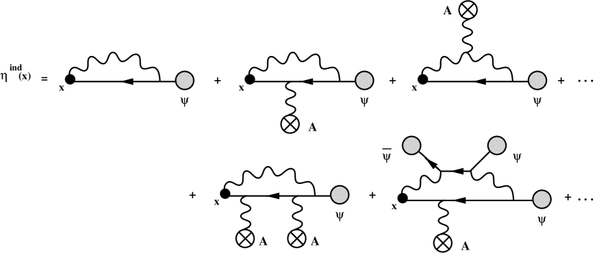
Figure 11: Some typical contributions to the induced fermionic source $\eta^{ind}$ in the one-loop approximation. The blobs represent either gauge field, or fermionic field insertions.

3.3.2 Gauge-covariant Wigner functions

As in the scalar theory in Sect. 2, the equations of motion for the 2-point functions are first rewritten in terms of Wigner functions, in order to facilitate the gradient expansion. If $G_{ab}(x,y)$ is a generic 2-point function, its Wigner transform reads (cf. eq. (2.136)):

$${\cal G}_{ab}(k,X)\,\equiv\,\int{\rm d}^{4}s\,{\rm e}^{ik\cdot s}G_{ab}\left(X+{s\over 2},X-{s\over 2}\right).$$ (3.71)

(From now on, we use calligraphic letters to denote the Wigner functions.) Unlike $G_{ab}(x,y)$, which is separately gauge-covariant at $x$ and $y$ (see, e.g., eq. (3.29)), its Wigner transform ${\cal G}_{ab}(k,X)$ — which mixes the two points $x$ and $y$ in its definition (3.71) — is not covariant. However, it is possible to construct a gauge covariant Wigner function. Consider first the following function:

$$\acute{G}_{ab}(s,X)\,\equiv\,U_{a\bar{a}}\Bigl{(}X,X+{s\over 2}\Bigr{)}\,G_{\bar{a}\bar{b}}\Bigl{(}X+{s\over 2},X-{s\over 2}\Bigr{)}\,U_{\bar{b}b}\Bigl{(}X-{s\over 2},X\Bigr{)},$$ (3.72)

where $U(x,y)$ is the non-Abelian parallel transporter, also referred to as a Wilson line:

$$U(x,y)={\rm P}\exp\left\{-ig\int_{\gamma}{\rm d}z^{\mu}A_{\mu}(z)\right\},$$ (3.73)

In eq. (3.73), $A_{\mu}^{a}=A_{\mu}^{a}T^{a}$, $\gamma$ is an arbitrary path going from $y$ to $x$, and the symbol P denotes the path-ordering of the colour matrices in the exponential. Under the gauge transformations of $A_{\mu}$, the Wilson line (3.73) transforms as (in matrix notations):

$$U(x,y)\longrightarrow h(x)\,U(x,y)\,h^{\dagger}(y),$$ (3.74)

so that the function (3.72) is gauge-covariant at $X$ for any given $s$:

$$\acute{G}(s,X)\longrightarrow h(X)\,\acute{G}(s,X)\,h^{\dagger}(X)\,.$$ (3.75)

Correspondingly, its Wigner transform

$$\acute{\cal G}_{ab}(k,X)\,\equiv\,\int{\rm d}^{4}s\,{\rm e}^{ik\cdot s}\,\acute{G}_{ab}(s,X)$$ (3.76)

transforms covariantly as well: For any given $k$, $\acute{\cal G}(k,X)\longrightarrow h(X)\,\acute{\cal G}(k,X)\,h^{\dagger}(X)$. In principle, any of the two Wigner functions (3.71) and (3.76) could be used to compute the induced sources (3.2.3). However, only the new Wigner function in eq. (3.76) will satisfy a gauge-covariant equation of motion, which makes its physical interpretation more transparent.

From now on, we shall use systematically gauge-covariant Wigner functions, denoted as $\acute{\cal S}(k,X)$, or $\acute{\cal G}_{\mu\nu}(k,X)$, $\acute{\cal K}(k,X)$. For instance,

$$\acute{\cal K}_{ia}^{\nu}(k,X)\equiv\int{\rm d}^{4}s\,{\rm e}^{ik\cdot s}\,U_{ij}\Bigl{(}X,X+{s\over 2}\Bigr{)}\,K^{\nu}_{jb}\Bigl{(}X+{s\over 2},X-{s\over 2}\Bigr{)}\,\tilde{U}_{ba}\Bigl{(}X-{s\over 2},X\Bigr{)},\qquad$$ (3.77)

where $U$ ($\tilde{U}$) is the parallel transporter in the fundamental (adjoint) representation. Under the gauge transformation (3.60),

$$\acute{\cal K}_{i}^{a}(k,X) \longrightarrow h_{ij}(X)\,\acute{\cal K}^{b}_{j}(k,X)\,\tilde{h}_{ab}(X).$$ (3.78)

By using eq. (3.2.3), one can express the induced sources in terms of these Wigner functions:

$$j_{{\rm f}}^{\mu\,a}(X) = g\int{{\rm d}^{4}k\over(2\pi)^{4}}\,{\rm Tr}\,\Bigl{(}\gamma_{\mu}t^{a}\acute{\cal S}(k,X)\Bigr{)},$$ (3.79)

$$j^{\mu\,a}_{\rm g}(X) = g\,\Gamma^{\mu\rho\lambda\nu}\int{{\rm d}^{4}k\over(2\pi)^{4}}\,{\rm Tr}\,T^{a}\biggl{\{}k_{\lambda}\acute{\cal G}_{\rho\nu}(k,X)+{i\over 2}\Bigl{[}D_{\lambda}^{X},\,\acute{\cal G}_{\rho\nu}(k,X)\Bigr{]}\biggr{\}},$$ (3.80)

$$\eta^{ind}(X) = g\int{{\rm d}^{4}k\over(2\pi)^{4}}\,\gamma^{\mu}t^{a}\acute{\cal K}_{\mu}^{a}(k,X).$$ (3.81)

At this stage, the path $\gamma$ in the Wilson line (3.73) is still arbitrary. In particular, if $\gamma$ is chosen as the straight line joining $x$ and $y$, the transition from non-covariant to gauge-covariant Wigner functions, e.g., from eq. (3.71) to eq. (3.76), can be interpreted as the replacement of the canonical momentum $\hat{k}^{\mu}=i\partial_{s}$ by the kinetic momentum $\hat{p}^{\mu}=\hat{k}^{\mu}-gA^{\mu}(X)$ [52, 147, 148]. In fact, most of our results will be independent of the exact form of $\gamma$. This is so because we need $U(x,y)$ only in situations where $x$ is close to $y$, as we argue now.

For soft and relatively weak background fields, the function $\acute{G}(s,X)$ remains close to its value in equilibrium, so it is peaked at $s=0$, and vanishes when $s\mathrel{\hbox to0.0pt{\raise 2.20013pt\hbox{$>$}\hss}{\lower 2.20013pt\hbox{$\sim$}}}1/T$. Over such a short scale, the mean field $A_{\mu}$ does not vary significantly, and we can write, for any path $\gamma$ joining $x$ and $y$,

$$g\int_{\gamma}{\rm d}z^{\mu}A_{\mu}(z)\,\approx\,g\bigl{(}s\cdot A(X)\bigr{)},$$ (3.82)

up to terms which involve, at least, one soft derivative $\partial_{X}A\sim gTA$ (and which do depend upon the path). Furthermore, for $s\sim 1/T$, $gs\cdot A\sim g$ (since $gA\sim gT$), so we can expand the exponential in eq. (3.73) in powers of $g$ and get, to leading non-trivial order,

$$U_{ab}(x,y)\,\simeq\,\delta_{ab}\,-\,ig\Bigl{(}s\cdot A_{ab}(X)\Bigr{)}.$$ (3.83)

The present use of the Wilson line should be contrasted with that in Sect. 3.1, where the parallel transporter in eq. (3.12) covers a relatively large space-time separation $|x-y|\sim 1/gT$ determined by the inhomogeneity in the system. In that case, the parallel transporter cannot be expanded as in eq. (3.83), for the reasons explained in Sect. 3.1. However, the corresponding path $\gamma$ is then fixed by the dynamics of the hard particles (cf. Sect. 4.1.1).

The constraint on the amplitudes of the mean fields entails a similar constraint on the off-equilibrium deviation $\delta G\equiv G-G_{eq}\/$: as we shall see later, $\delta G\sim(gA/T)G_{eq}\sim gG_{eq}$. Thus, by writing

$$G\equiv G_{eq}+\delta G,\qquad\qquad\acute{G}\equiv G_{eq}+\delta\acute{G},$$ (3.84)

in eq. (3.72), and recalling that $G_{eq}^{ab}=\delta^{ab}G_{eq}$, we can easily obtain the following relation between $\delta\acute{G}$ and $\delta G$, valid to leading order in $g$:

$$\delta\acute{G}(s,X)\,\simeq\,\delta G(x,y)\,+\,ig\Bigl{(}s\cdot A(X)\Bigr{)}G_{eq}(s),$$ (3.85)

or, after a Wigner transform,

$$\delta\acute{\cal G}(k,X)\simeq\delta{\cal G}(k,X)+g(A(X)\cdot\partial_{k})G_{eq}(k).$$ (3.86)

For an abnormal Wigner function, the equilibrium contribution vanishes, so that ordinary and gauge-covariant Wigner functions coincide to leading order in $g$ : e.g., $\acute{\cal K}_{\nu}\simeq{\cal K}_{\nu}$. Similar simplifications can be performed on eq. (3.80) for the gluonic current, to get:

$$j^{\mu\,a}_{\rm g}(X) = g\int{{\rm d}^{4}k\over(2\pi)^{4}}\,{\rm Tr}\,T^{a}\Bigl{\{}-k^{\mu}\delta\acute{\cal G}_{\nu}^{\,\,\,\nu}(k,X)+\delta\acute{\cal G}^{\mu\nu}(k,X)k_{\nu}\Bigr{\}},\,\,\,\,$$ (3.87)

where the following property has been used:

$$D^{\mu}_{x}G(x,y)\Big{|}_{y=x}\,=\,\partial^{\mu}_{s}\acute{G}(s,X)\Big{|}_{s=0}.$$ (3.88)

Note finally that, within the same approximations, the gauge-fixing conditions (3.3.1) imply that the gauge-covariant gluon Wigner function is (spatially) transverse, as at tree-level, $k^{i}\delta\acute{\cal G}_{i\nu}=0$, and similarly $k^{i}\acute{\cal K}_{i}=k^{i}\acute{\cal H}_{i}=0$. We can thus write:

$$\delta\acute{\cal G}_{ij}(k,X)\,\equiv\,(\delta_{ij}-\hat{k}_{i}\hat{k}_{j})\delta\acute{\cal G}(k,X)\,.$$ (3.89)

As we shall verify in Sect. 3.4.1, the spatial components above are the only ones to contribute to the induced current to leading order in $g$ (this is specific to Coulomb’s gauge [23, 26]). Thus, finally,

$$j^{a}_{{\rm g}\,\mu}(X)\,=\,2g\int{{\rm d}^{4}k\over(2\pi)^{4}}\,k_{\mu}{\rm Tr}\Bigl{\{}T^{a}\delta\acute{\cal G}(k,X)\Bigr{\}},$$ (3.90)

where the overall factor of 2 comes from the sum over transverse polarization states.

3.3.3 Gauge-covariant gradient expansion

In this section, we show how to extract the terms of leading order in $g$ in eqs. (3.65)–(3.3.1). This involves approximations similar to those already performed in the previous subsection (in relation with eqs. (3.83), (3.86) and (3.87)), and which take into account the dependence on $g$ associated with the soft inhomogeneities ($\partial_{X}\sim gT$), the amplitudes of the mean fields ($A\sim T$ or $F_{\mu\nu}\sim gT^{2}$), and the magnitude of the off-equilibrium deviations $\delta\acute{\cal G}\sim gG_{0}$. Since these approximations are related by gauge symmetry, we shall refer to them globally as the gauge-covariant gradient expansion.

Consider then the gluon 2-point function $G^{<\,ab}_{\mu\nu}(x,y)$ in the presence of a soft background field $A^{\mu}_{a}$, but without fermionic fields ($\Psi=\bar{\Psi}=0$). Like in the scalar theory in Sect. 2.3.2, we start with the following two Kadanoff-Baym equations for $G\equiv G^{<}$ (here, in the mean field approximation; cf. eq. (3.3.1)) :

$$\left(g_{\mu}^{\,\,\rho}D^{2}-D_{\mu}D^{\rho}+2igF_{\mu}^{\,\,\rho}\right)_{x}G_{\rho\nu}(x,y) = 0,$$

$$G_{\mu}^{\,\,\rho}(x,y)\left(g_{\rho\nu}\bigl{(}D^{\dagger}\bigr{)}^{2}-D_{\rho}^{\dagger}D_{\nu}^{\dagger}+2igF_{\rho\nu}\right)_{y} = 0,$$ (3.91)

and take their difference. This involves, in particular,

$$\Xi(x,y)\equiv D^{2}_{x}G(x,y)\,-\,G(x,y)(D^{\dagger}_{y})^{2},$$ (3.92)

where $D_{x}^{2}\,=\,\partial_{x}^{2}+2igA\cdot\partial_{x}+ig(\partial\cdot A)-g^{2}A^{2}\/$, and Minkowski indices are omitted to simplify the writing (they will be reestablished when needed). In this subsection we shall illustrate our approximations by focusing on $\Xi$.

After replacing the coordinates $x^{\mu}$ and $y^{\mu}$ by $s^{\mu}$ and $X^{\mu}$ (cf. eqs. (2.135) and (2.139)), we have, typically, $s\sim 1/T$, $\partial_{s}\sim T$ and $\partial_{X}\sim gT$. We then perform an expansion in powers of $\partial_{X}$ and keep only terms which involve, at most, one soft derivative $\partial_{X}$. For instance,

$$A_{\mu}(X+s/2)\approx A_{\mu}(X)+(1/2)(s\cdot\partial_{X})A_{\mu}(X).$$

Proceeding as in Sect. 2.3.2, and paying attention to the colour algebra, we obtain:

$$\Xi(s,X) = 2\partial_{s}\cdot\partial_{X}G+2ig\Bigl{[}A_{\mu}(X),\partial^{\mu}_{s}G\Bigr{]}+ig\Bigl{\{}A_{\mu}(X),\partial^{\mu}_{X}G\Bigr{\}}+ig\Bigl{\{}(s\cdot\partial_{X})A_{\mu},\partial^{\mu}_{s}G\Bigr{\}}$$ (3.93)

$$+ig\Bigl{\{}(\partial_{X}\cdot A),G\Bigr{\}}-g^{2}\left[A^{2}(X),G\right]-{g^{2}\over 2}\left\{(s\cdot\partial_{X})A^{2},G\right\}\,+\,...\,,$$

where the right parentheses (the braces) denote commutators (anticommutators) of colour matrices, and the dots stand for terms which involve at least two soft derivatives $\partial_{X}$.

At this point, we use the fact that $A\sim gT$ and $\delta G\equiv G-G_{eq}\,\sim\,gG_{eq}$ (as it will be verified a posteriori), with $G_{eq}\approx G_{0}$ in the present approximation (cf. eq. (3.70)). By keeping only terms of leading order in $g$, one simplifies eq. (3.93) to:

$$\Xi(s,X)\approx 2(\partial_{s}\cdot\partial_{X})\delta G+2ig\left[A_{\mu},\partial^{\mu}_{s}\delta G\right]+2ig(s\cdot\partial_{X})A_{\mu}\,(\partial^{\mu}_{s}G_{0})+2ig(\partial_{X}\cdot A)G_{0},\,\,$$ (3.94)

where all the terms in the r.h.s. are of order $g^{2}T^{2}G_{0}$. After a Fourier transform with respect to $s$, $\,\Xi(s,X)$ becomes $-i\,\Xi(k,X)$ with:

$$\Xi(k,X)\,\approx\,2\Bigl{[}k\cdot D_{X},\,\delta{\cal G}(k,X)\Bigr{]}+2gk^{\mu}\Bigl{(}\partial_{X}^{\nu}A_{\mu}(X)\Bigr{)}\partial_{\nu}G_{0}(k).$$ (3.95)

Here, $\delta{\cal G}(k,X)$ is the ordinary Wigner transform of $\delta G(x,y)$, eq. (3.71), but it can be expressed in terms of the gauge-covariant Wigner function $\delta\acute{\cal G}(k,X)$ with the help of eq. (3.86). This finally yields:

$$\Xi_{\mu\nu}(k,X)\,\approx\,2\Bigl{[}k\cdot D_{X},\delta\acute{\cal G}_{\mu\nu}(k,X)\Bigr{]}-2gk^{\alpha}F_{\alpha\beta}(X)\,\partial^{\beta}G_{\mu\nu}^{(0)}(k),$$ (3.96)

where the Minkowski indices have been reintroduced.

We recognize here the familiar structure of the Vlasov equation, generalized to a non-Abelian plasma: Eq. (3.96) involves a (gauge-covariant) drift term $(k\cdot D_{X})\delta\acute{\cal G}$, together with a “force term” proportional to the background field strength tensor. In fact, this “force term” involves the equilibrium distribution function $G_{0}\equiv G^{<}_{0}$, so, in this respect, it is closer to the linearized version of the Vlasov equation, eq. (1.13). However, unlike eq. (1.13), its non-Abelian counterpart in eq. (3.96) is still non-linear, because of the presence of the covariant drift operator $(k\cdot D_{X})$, and because the non-Abelian field strength tensor is itself non-linear.

3.4 The non-Abelian Vlasov equations

In this section, we construct the kinetic equations which determine the colour current induced by a soft gauge field $A^{\mu}_{a}$. (The fermionic mean fields $\Psi$ and $\bar{\Psi}$ are set to zero in what follows.) According to eqs. (3.79) and (3.90), we need the equations satisfied by the quark and gluon Wigner functions, $\delta\acute{\cal S}$ and $\delta\acute{\cal G}_{\mu\nu}$, in the presence of the background field $A^{\mu}_{a}$. From the discussion in the previous subsection, we anticipate that these equations are non-Abelian generalizations of the (linearized) Vlasov equation.

3.4.1 Vlasov equation for gluons

Since we expect the transverse components $\delta\acute{\cal G}_{ij}$ to be the dominant ones, we focus on the spatial components ($\mu=i$ and $\nu=j$) of eqs. (3.3.3):

$$D_{x}^{2}G_{ij}-D^{x}_{i}D^{x}_{0}G_{0j}+2igF_{i}^{\,\rho}(x)G_{\rho j} = 0,$$

$$G_{ij}\Bigl{(}D_{y}^{\dagger}\Bigr{)}^{2}-G_{i0}D_{0\,y}^{\dagger}D_{j\,y}^{\dagger}+2igG_{i\rho}F^{\rho}_{\,\nu}(y) = 0.$$ (3.97)

(We have also used eq. (3.3.1) to simplify some terms in these equations.) We now take their difference, to be succinctly referred to as the difference equation (cf. Sect. 2.3.2). In doing so, we first meet (cf. eqs. (3.92) and (3.96)):

$$D_{x}^{2}G_{ij}-G_{ij}\Bigl{(}D_{y}^{\dagger}\Bigr{)}^{2}\,\longrightarrow\,2\Bigl{[}k\cdot D_{X},\delta\acute{\cal G}_{ij}\Bigr{]}-2gk^{\alpha}F_{\alpha\beta}(X)\,\partial^{\beta}G^{(0)}_{ij}(k).$$ (3.98)

Note the following identity, which will be useful later:

$$k^{\alpha}F_{\alpha\beta}\partial^{\beta}G^{(0)}_{ij}(k)\equiv k^{\alpha}F_{\alpha\beta}\partial^{\beta}[(\delta_{ij}-\hat{k}_{i}\hat{k}_{j})G_{0}(k)]$$ (3.99)

$$=(\delta_{ij}-\hat{k}_{i}\hat{k}_{j})k^{\alpha}F_{\alpha\beta}\partial^{\beta}G_{0}-k^{\alpha}F_{\alpha l}\,{k_{i}\delta_{jl}+k_{j}\delta_{il}-2\hat{k}_{i}\hat{k}_{j}k_{l}\over{\bf k}^{2}}\,G_{0}.\,\,\,$$

This shows that the r.h.s. of eq. (3.98) involves also non-transverse components. These will be canceled by the other terms in eqs. (3.4.1), as we explain now.

The components $G_{i0}$ and $G_{0j}$ vanish in equilibrium, and remain small out of equilibrium (see below), but nevertheless their contribution to the difference equation is non-negligible. This is so since the hard derivatives $\partial^{s}_{0}\partial^{s}_{i}\sim T^{2}$ multiplying these components do not cancel in the difference equation, in contrast to what happens in the terms involving $\delta G_{ij}$ (cf. eq. (3.98), where we remember that $\partial_{x}^{2}-\partial_{y}^{2}=2\partial_{s}\cdot\partial_{X}\sim gT^{2}$). One can evaluate these components from eqs. (3.3.3) with $\mu=0$ and $\nu=j\/$. This gives [26] :

$${\cal G}_{0j}(k,X)\,\approx\,2igF_{0l}\,{\delta_{lj}-\hat{k}_{l}\hat{k}_{j}\over{\bf k}^{2}}\,G_{0}(k),\qquad{\cal G}_{i0}^{ab}(k,X)={\cal G}_{0i}^{ba}(-k,X),$$ (3.100)

which provides the following contribution to the difference equation:

$$-\Bigl{(}D^{x}_{i}D^{x}_{0}G_{0j}-G_{i0}D_{0\,y}^{\dagger}D_{j\,y}^{\dagger}\Bigr{)}\,\longrightarrow\,-2gk^{0}F_{0l}(X)\,{k_{i}\delta_{jl}+k_{j}\delta_{il}-2\hat{k}_{i}\hat{k}_{j}k_{l}\over{\bf k}^{2}}\,G_{0}(k).$$ (3.101)

Finally, there is a contribution from the terms involving the field strength tensor in eqs. (3.4.1). To the order of interest, it reads:

$$-2ig\Bigl{(}F_{il}(X)G_{lj}^{(0)}(s)-G_{il}^{(0)}(s)F_{lj}(X)\Bigr{)}\,\longrightarrow\,-2gG_{0}(k)\Bigl{(}F_{il}\hat{k}_{l}\hat{k}_{j}+F_{jl}\hat{k}_{l}\hat{k}_{i}\Bigr{)}.$$ (3.102)

Together, the contributions in eqs. (3.101) and (3.102) precisely cancel the non-transverse piece in the r.h.s. of eq. (3.98), as anticipated.

To conclude, $\delta\acute{\cal G}_{ij}$ is transverse indeed, as required by the gauge condition (3.89), and can be written as $\delta\acute{\cal G}_{ij}=(\delta_{ij}-\hat{k}_{i}\hat{k}_{j})\delta\acute{\cal G}$, with $\delta\acute{\cal G}(k,X)$ satisfying:

$$\Bigl{[}k\cdot D_{X},\,\delta\acute{\cal G}(k,X)\Bigr{]}\,=\,g\,k^{\alpha}F_{\alpha\beta}(X)\partial^{\beta}G_{0}(k).$$ (3.103)

Since $D_{X}\sim gT$ and $gF_{\alpha\beta}\sim(D_{X})^{2}\sim g^{2}T^{2}$, it follows that $\delta\acute{\cal G}\sim(D_{X}/T)G_{0}\sim gG_{0}$, as anticipated. (By comparison, ${\cal G}_{0j}\sim(gF_{0i}/T^{2})G_{0}\sim g^{2}G_{0}$ is of higher order in $g$.)

Since $G_{0}\equiv G^{<}_{0}(k)=2\pi\epsilon(k_{0})\delta(k^{2})N(k_{0})$, and therefore

$$k^{\alpha}F_{\alpha\beta}\partial_{k}^{\beta}G_{0}(k)\,=\,2\pi\delta(k^{2})k^{i}F_{i0}({\rm d}N/{\rm d}k_{0}),$$ (3.104)

it follows that $\delta\acute{\cal G}(k,X)$ has support only on the tree-level mass-shell $k^{2}=0$. By also using the symmetry property (3.58), we can write:

$$\delta\acute{\cal G}_{ab}(k,X) \equiv 2\pi\delta(k^{2})\Bigl{\{}\theta(k_{0})\delta N_{ab}({\bf k},X)\,+\,\theta(-k_{0})\delta N_{ba}(-{\bf k},X)\Bigr{\}},$$ (3.105)

where $\delta N_{ab}({\bf k},X)$ is a density matrix satisfying the following, Vlasov-type, equation [23] (with $v^{\mu}=(1,{\bf k}/k)$ and $E^{i}=F^{i0}=E^{i}_{a}T^{a}$):

$$\left[v\cdot D_{X},\,\delta N({{\bf k}},X)\right]=-\,g\,{\bf v}\cdot{\bf E}(X){{\rm d}N\over{\rm d}k}\,.$$ (3.106)

This equation implies that $\delta N$ has the same colour structure as the electric field ${\bf E}(x)$, that is, $\delta N\equiv\delta N^{a}T^{a}$, with the components $\delta N^{a}({\bf k},x)$ transforming as a colour vector in the adjoint representation. In terms of this density matrix, the induced current (3.90) can be finally written as :

$$j^{A\,a}_{{\rm g}\,\mu}(X)\,=\,2g\int{{\rm d}^{3}k\over(2\pi)^{3}}\,v_{\mu}\,{\rm Tr}\Bigl{(}T^{a}\delta N({\bf k},X)\Bigr{)}\,=\,2gN\int{{\rm d}^{3}k\over(2\pi)^{3}}\,v_{\mu}\,\delta N^{a}({\bf k},X).$$ (3.107)

Aside from its covariance under the gauge transformations of the background field, eq. (3.106) is also independent of the gauge-fixing for the quantum fields, as proven in Ref. [23].

3.4.2 Vlasov equation for quarks

We now briefly consider the corresponding equation for the quark 2-point function $S\equiv S^{<}$. Starting with eq. (3.65), namely

$$\hbox to0.0pt{\hbox to8.55695pt{\hfil/\hfil}\hss}D_{x}S(x,y)\,=\,0,\qquad S(x,y)\hbox to0.0pt{\hbox to8.55695pt{\hfil/\hfil}\hss}D^{\dagger}_{y}\,=\,0,$$ (3.108)

and using (with $\sigma^{\mu\nu}\equiv(i/2)[\gamma^{\mu},\gamma^{\nu}]$)

$$\hbox to0.0pt{\hbox to8.55695pt{\hfil/\hfil}\hss}D_{x}\,\hbox to0.0pt{\hbox to8.55695pt{\hfil/\hfil}\hss}D_{x}=\,D_{x}^{2}+{g\over 2}\,\sigma^{\mu\nu}F_{\mu\nu}(x),$$ (3.109)

one obtains the following difference equation:

$$D_{x}^{2}S(x,y)-S(x,y)\bigl{(}D_{y}^{\dagger})^{2}+{g\over 2}\,\Bigl{(}\sigma^{\mu\nu}F_{\mu\nu}(x)S(x,y)-S(x,y)\sigma^{\mu\nu}F_{\mu\nu}(y)\Bigr{)}=0.\,\,\,\,$$ (3.110)

Then one proceeds with a gauge-covariant gradient expansion, as in Sect. 3.3.3, which finally yields the following equation for the covariant Wigner function $\delta\acute{\cal S}(k,X)$ (valid to leading order in $g$):

$$\left[k\cdot D_{X},\,\delta\acute{\cal S}(k,X)\right]=gk\cdot F(X)\cdot\partial_{k}S_{0}^{<}-i\,{g\over 4}\,F^{\mu\nu}(X)\Bigl{[}\sigma_{\mu\nu},\,S_{0}\Bigr{]}.$$ (3.111)

By also using $S_{0}\equiv S_{0}^{<}(k)=\hbox to0.0pt{\hbox to5.52084pt{\hfil/\hfil}\hss}k\tilde{\Delta}(k)\equiv\hbox to0.0pt{\hbox to5.52084pt{\hfil/\hfil}\hss}k\rho_{0}(k)n(k^{0})$ (cf. eq. (3.56)), and calculating the Dirac commutator $[\sigma_{\mu\nu},\hbox to0.0pt{\hbox to5.52084pt{\hfil/\hfil}\hss}k]$, we finally get the simple equation:

$$\left[k\cdot D_{X},\,\delta\acute{\cal S}(k,X)\right]=g\,\hbox to0.0pt{\hbox to5.52084pt{\hfil/\hfil}\hss}k\,k\cdot F(X)\cdot\partial_{k}\tilde{\Delta}(k),$$ (3.112)

which implies that $\delta\acute{\cal S}$ is a colour matrix of the form $\delta\acute{\cal S}=\delta\acute{\cal S}_{a}t^{a}$, with the components $\delta\acute{\cal S}_{a}$ transforming as a colour vector. Eq. (3.112) also shows that $\delta\acute{\cal S}$ has the same spin and mass-shell structure as the free 2-point function $S_{0}^{<}$:

$$\delta\acute{\cal S}(k,X)\,=\,\hbox to0.0pt{\hbox to5.52084pt{\hfil/\hfil}\hss}k\,2\pi\delta(k^{2})\left\{\theta(k_{0})\delta n_{+}({\bf k},X)+\theta(-k_{0})\delta n_{-}(-{\bf k},X)\right\}.$$ (3.113)

The density matrices $\delta n_{\pm}({\bf k},X)\equiv\delta n_{\pm}^{a}({\bf k},X)\,t^{a}$ satisfy the following kinetic equation:

$$\left[v\cdot D_{X},\,\delta n_{\pm}({{\bf k}},X)\right]=\mp\,g\,{\bf v}\cdot{\bf E}(X)\,{{\rm d}n_{k}\over{\rm d}k},$$ (3.114)

which is the non-Abelian version of the Vlasov equation for quarks. The induced current $j_{\rm f\,\mu}^{A\,a}$ reads finally (cf. eq. (3.79)):

$$j_{{\rm f}\,\mu}^{A\,a}(X) = gN_{f}\int{{\rm d}^{3}k\over(2\pi)^{3}}\,v_{\mu}\Bigl{(}\delta n_{+}^{a}({\bf k},X)-\delta n_{-}^{a}({\bf k},X)\Bigr{)}.$$ (3.115)

3.5 Kinetic equations for the fermionic excitations

A noteworthy feature of the ultrarelativistic plasmas is the existence of collective modes with fermionic quantum numbers. The associated collective motion involves both quarks and gluons, whose mutual transformations, over a long space-time range, can be described as a propagating fermionic field $\Psi(x)$ [18, 23]. We shall now establish the kinetic equations which determine the corresponding induced sources $\eta^{ind}$ and $j_{\mu}^{\psi}$.

3.5.1 Equation for $\eta^{ind}$

The fermionic source $\eta^{ind}(x)$ is given by eq. (3.81), where, to the order of interest, we can replace the gauge covariant Wigner function $\acute{\cal K}_{\mu}^{a}(k,X)$ by the ordinary Wigner transform ${\cal K}_{\mu}^{a}(k,X)$ (cf. after eq. (3.85)). The kinetic equation for ${\cal K}_{\mu}^{a}(k,X)$ is obtained from the equations of motion (3.66) and (3.67) for $K^{a}_{\mu}(x,y)$, that is

$$\hbox to0.0pt{\hbox to8.55695pt{\hfil/\hfil}\hss}D_{x}K_{\mu}^{a}(x,y) = -igt^{a}\gamma^{\nu}\Psi(x)G^{(0)}_{\nu\mu}(x,y),$$ (3.116)

$$\Bigl{(}g_{\mu\nu}\tilde{D}^{2}-\tilde{D}_{\mu}\tilde{D}_{\nu}+2ig\tilde{F}_{\mu\nu}\Bigr{)}_{y}^{ab}K^{\nu}_{b}(x,y) = -gS_{0}(x,y)\gamma_{\mu}t^{a}\Psi(y),$$ (3.117)

where $D$ ($\tilde{D}$) is the covariant derivative in the fundamental (adjoint) representation. (To simplify notations, the colour indices for the fundamental representation are not shown explicitly; see, e.g., eq. (3.2.3).) These equations describe a process where a hard gluon scatters off a soft fermionic field $\Psi$ and gets “turned into” a hard quark, or a hard antiquark annihilates against $\Psi$ to generate a hard gluon.

In the right hand sides of the above equations, we have replaced the full gluon and fermion propagators $G_{\nu\mu}$ and $S$ by their free counterparts $G^{(0)}_{\nu\mu}$ and $S_{0}$. This is correct in leading order since the off-equilibrium deviations are suppressed by one power of $g\/$: e.g., $\delta S\sim gS_{0}$. (For the deviations induced by the fermionic fields, this relies on the constraint $\bar{\Psi}\Psi\sim gT^{3}$; see Sect. 3.5.2 below.) Because of that, these equations are linear in $\Psi$, although non-linear in $A^{\mu}_{a}$.

As for the gluon Wigner function in in Sect. 3.4.1, here too there is a hierarchy among the components of ${\cal K}_{\mu}^{a}(k,X)$: The spatial components ${\cal K}_{i}^{a}$ are the large ones, and are transverse: $k^{i}{\cal K}_{i}=0$. The temporal component ${\cal K}_{0}^{a}$ is smaller, ${\cal K}_{0}\sim g{\cal K}_{i}$, so it does not contribute to the induced source $\eta^{ind}$ directly; its only role is to remove the longitudinal component of the r.h.s. of eq. (3.116). (Thus, $K_{0}$ plays here the same role as $G_{0j}$ in Sect. 3.4.1.) Then eq. (3.116) with $\mu=i$ reduces to:

$$(\tilde{D}_{y}^{2})^{ab}K_{i}^{b}(x,y)\,=\,-gS^{(0)}_{ij}(x-y)\gamma^{j}t^{a}\Psi(y),$$ (3.118)

where

$$S^{(0)}_{ij}(s)\equiv\int{{\rm d}^{4}k\over(2\pi)^{4}}\,{\rm e}^{-ik\cdot s}(\delta_{ij}-\hat{k}_{i}\hat{k}_{j})S_{0}(k).$$ (3.119)

To the same order, eq. (3.116) simplifies to

$$D^{2}_{x}K^{a}_{i}(x,y)\,\approx\,-igt^{a}\gamma^{\lambda}\gamma^{j}\Psi(x)\partial^{x}_{\lambda}G^{(0)}_{ji}(x-y),$$ (3.120)

where the r.h.s. is transverse indeed (cf. eq. (3.42)).

We now subtract eq. (3.118) from eq. (3.120) and transform the difference equation as in the previous subsections. One then finds, for instance,

$$\Bigl{(}D^{2}_{x}\delta^{ab}-(\tilde{D}_{y}^{2})^{ab}\Bigr{)}K^{b}_{i}(x,y)\,\approx\,2\Bigl{(}(\partial_{X}+igA(X))\delta^{ab}+ig\tilde{A}^{ab}(X)\Bigr{)}\cdot\partial_{s}K^{b}_{i}(s,X),$$ (3.121)

which, in contrast to eq. (3.94), does not involve the soft derivative $\partial_{X}A$ of the background gauge field (this is so since $K^{a}_{\mu}$ vanishes in equilibrium). Thus, there will be no “Lorentz force” in the kinetic equation for ${\cal K}_{i}^{a}(k,X)$, which finally reads:

$$k\cdot\left[(\partial_{X}+igA(X))\delta^{ab}+ig\tilde{A}^{ab}(X)\right]{\cal K}^{b}_{i}(k,X)\,=\qquad\qquad\qquad$$

$$\qquad=\,-i{g\over 2}\,\rho_{0}(k)\Bigl{(}N(k_{0})+n(k_{0})\Bigr{)}\hbox to0.0pt{\hbox to5.52084pt{\hfil/\hfil}\hss}k\gamma^{j}(\delta_{ij}-\hat{k}_{i}\hat{k}_{j})t^{a}\Psi(X).$$ (3.122)

The differential operator in the l.h.s. is a covariant derivative acting on vectors in the direct product of the fundamental and the adjoint representation. Thus, eq. (3.5.1) is consistent with the transformation law (3.78) for ${\cal K}^{a}_{i}(k,X)$. In a pictorial representation of the solution ${\cal K}_{i}^{a}(k,X)$, the fundamental gauge field $A^{\mu}=A^{\mu}_{a}t^{a}$ (respectively, the adjoint field $\tilde{A}^{\mu}=A^{\mu}_{a}T^{a}$) in the l.h.s. of eq. (3.5.1) is responsible for gauge field insertions along the external quark leg (respectively, gluon leg) of ${\cal K}_{i}^{a}$ (cf. fig. 12).

Figure 12: Pictorial representation of the solution ${\cal K}^{a}_{i}(k,X)$ to eq. (3.5.1): $A$ ($\tilde{A}$) denotes insertions of the gauge mean field in the fundamental (adjoint) representation.

The induced source (3.81) involves the quantity ${\cal{\hbox to0.0pt{\hbox to9.20833pt{\hfil/\hfil}\hss}K}}(k,X)\equiv t^{a}\gamma^{\mu}{\cal K}_{\mu}^{a}\approx t^{a}\gamma^{i}{\cal K}_{i}^{a}$. To get the equation satisfied by this quantity, multiply eq. (3.5.1) by $t^{a}$ from the left, and use the identities $t^{a}t^{c}+if^{abc}t^{b}=t^{c}t^{a}$ and $t^{a}t^{a}=(N^{2}-1)/2N\equiv C_{\rm f}$ to obtain:

$$\left(k\cdot D_{X}\right){\cal{\hbox to0.0pt{\hbox to9.20833pt{\hfil/\hfil}\hss}K}}(k,X)=-ig{d-2\over 2}C_{\rm f}\rho_{0}(k)\Bigl{(}N(k_{0})+n(k_{0})\Bigr{)}\hbox to0.0pt{\hbox to5.52084pt{\hfil/\hfil}\hss}k\Psi(X).$$ (3.123)

The factor $(d-2)=2$ — which arises via $\gamma^{i}\hbox to0.0pt{\hbox to5.52084pt{\hfil/\hfil}\hss}k\gamma^{j}(\delta_{ij}-\hat{k}_{i}\hat{k}_{j})=(d-2)\hbox to0.0pt{\hbox to5.52084pt{\hfil/\hfil}\hss}k$ — indicates that only the transverse gluons are involved in this collective motion. This is a consequence of the fact that eq. (3.123) is gauge-fixing independent, as actually proven in Refs. [18, 23].

Note that the adjoint gauge field $\tilde{A}^{ab}(X)$ has disappeared in going from eq. (3.5.1) to eq. (3.123): the latter involves only the covariant derivative in the fundamental representation, which is consistent with the fact that ${\cal{\hbox to0.0pt{\hbox to9.20833pt{\hfil/\hfil}\hss}K}}(k,X)$ must transform in the same way as $\Psi(X)$ under a gauge rotation of the background fields.

Since the r.h.s. of eq. (3.123) is proportional to $\rho(k)$, it follows that:

$${\cal{\hbox to0.0pt{\hbox to9.20833pt{\hfil/\hfil}\hss}K}}(k,X)=2\pi\delta(k^{2})\Bigl{\{}\theta(k_{0})\hbox to0.0pt{\hbox to6.94444pt{\hfil/\hfil}\hss}\Lambda({\bf k},X)+\theta(-k_{0})\hbox to0.0pt{\hbox to6.94444pt{\hfil/\hfil}\hss}\Lambda(-{\bf k},X)\Bigr{\}},$$ (3.124)

with the density matrix ${\hbox to0.0pt{\hbox to6.94444pt{\hfil/\hfil}\hss}\Lambda}({\bf k},X)$ satisfying (with $d=4$, and $v^{\mu}=(1,{\bf k}/k)$):

$$(v\cdot D_{X}){\hbox to0.0pt{\hbox to6.94444pt{\hfil/\hfil}\hss}\Lambda}({\bf k},X)=-igC_{\rm f}\,(N_{k}+n_{k})\,{\hbox to0.0pt{\hbox to5.20601pt{\hfil/\hfil}\hss}v}\,\Psi(X),$$ (3.125)

Finally, the fermionic source $\eta^{ind}(X)$ is obtained as:

$$\eta^{ind}(X)=g\,\int{{\rm d}^{3}k\over(2\pi)^{3}}{1\over\epsilon_{k}}\hbox to0.0pt{\hbox to6.94444pt{\hfil/\hfil}\hss}\Lambda({\bf k},X).$$ (3.126)

Eq. (3.125) is the analog of the Vlasov equation, the fermionic field playing in the former the same role as the colour electric field in the r.h.s. of the latter. There is, however, a noticeable difference: the equilibrium distributions $N_{k}$ and $n_{k}$ enter the r.h.s. of eq. (3.125), while their variations, ${\rm d}N/{\rm d}k$ and ${\rm d}n/{\rm d}k$, enter the r.h.s.’s of the Vlasov equations (3.106) and (3.114), respectively. This reflects the difference in the mechanism by which the hard particles react to the propagation of a colour field, or of a fermionic field. In the first case, the field slightly changes the momentum of the hard particles causing a modification of their distribution functions. In the second case, the basic mechanism at work is a conversion of hard gluons into hard fermions, or vice-versa, the soft fermionic field bringing the necessary quantum numbers, but no momentum.

The same mechanism acts also in QED, where the long-range fermionic excitations are described by eq. (3.125) with $gC_{\rm f}\to e$, and the non-Abelian covariant derivative $D_{\mu}=\partial_{\mu}+igt^{a}A^{a}_{\mu}$ replaced by the Abelian one, $D_{\mu}=\partial_{\mu}+ieA_{\mu}$ [18].

3.5.2 Equations for $j^{\psi}_{\mu}$

Since the background fermionic fields carry also colour, they induce a colour current $j_{\mu}^{\psi\,a}$ when acting of the hard particles. In the general equations (3.65) and (3.3.1) for $S$ and $G$, the effects of the fermionic fields $\Psi$ and $\bar{\Psi}$ are mixed with those of the gauge fields $A^{\mu}$. It is convenient to separate these effects, by writing

$$\acute{\cal S}(k,X)=S_{0}(k)+\delta\acute{\cal S}^{A}(k,X)+\delta{\cal S}^{\psi}(k,X),$$ (3.127)

together with a similar decomposition for $\acute{\cal G}_{\mu\nu}$. Here, $\delta\acute{\cal S}^{A}$, and similarly $\delta\acute{\cal G}_{\mu\nu}^{A}$, denote the off-equilibrium deviations induced by the gauge fields when $\Psi=\bar{\Psi}=0$, and obey the kinetic equations established in Sect. 3.4. The other pieces, $\delta{\cal S}^{\psi}$ and $\delta{\cal G}_{\mu\nu}^{\psi}$, denote the additional deviations which emerge in the presence of soft fermionic fields, and which are responsible for the piece $j_{\mu}^{\psi}$ of the induced current:

$$j_{\mu}^{\psi\,a}(X) = g\int{{\rm d}^{4}k\over(2\pi)^{4}}\,\left\{{\cal J}^{\psi\,a}_{{\rm f}\,\mu}(k,X)\,+\,{\cal J}^{\psi\,a}_{{\rm g}\,\mu}(k,X)\right\},$$ (3.128)

We have introduced here the following phase-space current densities (cf. eqs. (3.79) and (3.90)):

$${\cal J}^{\psi\,a}_{{\rm f}\,\mu}(k,X)\,\equiv\,{\rm Tr}\,\gamma_{\mu}t^{a}\delta{\cal S}^{\psi}(k,X),\qquad{\cal J}^{\psi\,a}_{{\rm g}\,\mu}(k,X)\,\equiv\,2k_{\mu}{\rm Tr}\,T^{a}\delta{\cal G}^{\psi}(k,X),$$ (3.129)

in terms of which the kinetic equations pertinent to $j_{\mu}^{\psi}$ are most conveniently written [18, 23] (with ${\cal{\hbox to0.0pt{\hbox to9.20833pt{\hfil/\hfil}\hss}K}}^{a}\equiv\gamma^{\mu}{\cal K}_{\mu}^{a}$, etc.):

$$\,\left[k\cdot D_{X},\,{\cal J}^{\psi}_{{\rm f}\,\mu}(k,X)\right]^{a} = igk_{\mu}\,\left\{\bar{\Psi}(X)\,t^{a}\,\hbox to0.0pt{\hbox to7.7778pt{\hfil/\hfil}\hss}{\cal K}(k,X)-\hbox to0.0pt{\hbox to7.50002pt{\hfil/\hfil}\hss}{\cal H}(k,X)\,t^{a}\,\Psi(X)\right\}$$ (3.130)

$$- i\,{g\over 2}Nk_{\mu}\left\{\bar{\Psi}(X)\,\hbox to0.0pt{\hbox to7.7778pt{\hfil/\hfil}\hss}{\cal K}^{a}(k,X)-\hbox to0.0pt{\hbox to7.50002pt{\hfil/\hfil}\hss}{\cal H}^{a}(k,X)\,\Psi(X)\right\},$$

$$\Bigl{[}k\cdot D_{X},\,{\cal J}^{\psi}_{{\rm g}\,\mu}(k,X)\Bigr{]}^{a} = i\,{g\over 2}\,N\,k_{\mu}\left\{\bar{\Psi}(X)\,\hbox to0.0pt{\hbox to7.7778pt{\hfil/\hfil}\hss}{\cal K}^{a}(k,X)-\hbox to0.0pt{\hbox to7.50002pt{\hfil/\hfil}\hss}{\cal H}^{a}(k,X)\,\Psi(X)\right\}.$$ (3.131)

These equations are gauge-fixing independent, and covariant with respect to the gauge transformations of the background fields. The expressions in their r.h.s.’s are bilinear in $\Psi$ and $\bar{\Psi}$, as necessary for the conservation of the fermionic quantum number. (The general equations satisfied by the off-equilibrium propagators $\delta{\cal S}^{\psi}$ and $\delta{\cal G}_{\mu\nu}^{\psi}$ can be found in [23], where it is also verified that, for $\bar{\Psi}\Psi\sim gT^{3}$, these deviations are perturbatively small: $\delta{\cal S}^{\psi}\sim gS_{0}$ and $\delta{\cal G}^{\psi}\sim gG_{0}$.)

Quite remarkably, the genuinely non-Abelian terms, proportional to $N$, in the right hand sides of these two equations cancel in their sum, that is, in the equation satisfied by the total current ${\cal J}_{\mu}^{\psi}\equiv{\cal J}^{\psi}_{{\rm f}\,\mu}+{\cal J}^{\psi}_{{\rm g}\,\mu}\/$, which reads simply:

$$\left[k\cdot D_{X},\,{\cal J}^{\psi}_{\mu}(k,X)\right]=igk_{\mu}\,t^{a}\left\{\bar{\Psi}(X)\,t^{a}\,\hbox to0.0pt{\hbox to7.7778pt{\hfil/\hfil}\hss}{\cal K}(k,X)-\hbox to0.0pt{\hbox to7.50002pt{\hfil/\hfil}\hss}{\cal H}(k,X)\,t^{a}\,\Psi(X)\right\}.$$ (3.132)

Thus, the total current ${\cal J}_{\mu}^{\psi}$ is effectively determined by the Abelian-like piece of the quark current ${\cal J}^{\psi}_{{\rm f}\,\mu}$ alone (i.e., the first term in the r.h.s. of eq. (3.130)). Not surprisingly then, eq. (3.132) has a direct analog in QED, which reads [18]

$$(k\cdot\partial_{X}){\cal J}^{\psi}_{\mu}(k,X)\,=\,igk_{\mu}\,\left\{\bar{\Psi}(X)\,\hbox to0.0pt{\hbox to7.7778pt{\hfil/\hfil}\hss}{\cal K}(k,X)-\hbox to0.0pt{\hbox to7.50002pt{\hfil/\hfil}\hss}{\cal H}(k,X)\,\Psi(X)\right\}.$$ (3.133)

Since the r.h.s. of eq. (3.132) (or (3.133)) has support only at $k^{2}=0$, the current can be expressed in terms of on-shell density matrices, as follows:

$${\cal J}^{\psi}_{\mu}(k,X)=2k_{\mu}\,2\pi\delta(k^{2})\left\{\theta(k^{0})\delta n^{\psi}_{+}({\bf k},X)+\theta(-k^{0})\delta n^{\psi}_{-}(-{\bf k},X)\right\}.$$ (3.134)

Note that the net contribution to the induced current ${\cal J}_{\mu}^{\psi}$ is due to the hard fermions only, because of the cancellations alluded to before.

The colour density matrices $\delta n_{\pm}^{\psi}=\delta n_{\pm}^{\psi\,a}t^{a}$ satisfy the following kinetic equation (with $\bar{\hbox to0.0pt{\hbox to6.94444pt{\hfil/\hfil}\hss}\Lambda}\equiv{\hbox to0.0pt{\hbox to6.94444pt{\hfil/\hfil}\hss}\Lambda}^{\dagger}\gamma^{0}$) :

$$\Bigl{[}v\cdot D_{X},\,\delta n_{\pm}^{\psi}({\bf k},X)\Bigr{]}^{a}=\pm i\,{g\over 2\epsilon_{k}}\left\{\bar{\Psi}(X)\,t^{a}{\hbox to0.0pt{\hbox to6.94444pt{\hfil/\hfil}\hss}\Lambda}({\bf k},X)-\bar{\hbox to0.0pt{\hbox to6.94444pt{\hfil/\hfil}\hss}\Lambda}({\bf k},X)\,t^{a}\Psi(X)\right\}.$$ (3.135)

In terms of them, the induced current $j_{\mu}^{\psi}$ is finally written as:

$$j_{\mu}^{\psi\,a}(X)\,=\,2g\int{{\rm d}^{3}k\over(2\pi)^{3}}\,v_{\mu}\,{\rm Tr}\,t^{a}\left(\delta n_{+}^{\psi}({\bf k},X)-\delta n_{-}^{\psi}({\bf k},X)\right).$$ (3.136)

3.6 Summary of the kinetic equations

Let us summarize now the kinetic equations which represent the main result of this section. These are written here for the various density matrices, and read (cf. eqs. (3.114), (3.106), (3.125), and (3.135)) :

$$\left[v\cdot D_{x},\,\delta n_{\pm}({{\bf k}},x)\right] = \mp\,g\,{\bf v}\cdot{\bf E}(x)\,{{\rm d}n_{k}\over{\rm d}k},$$ (3.137)

$$\left[v\cdot D_{x},\,\delta N({{\bf k}},x)\right] = -\,g\,{\bf v}\cdot{\bf E}(x){{\rm d}N_{k}\over{\rm d}k},$$ (3.138)

$$(v\cdot D_{x}){\hbox to0.0pt{\hbox to6.94444pt{\hfil/\hfil}\hss}\Lambda}({\bf k},x) = -igC_{\rm f}\,(N_{k}+n_{k})\,{\hbox to0.0pt{\hbox to5.20601pt{\hfil/\hfil}\hss}v}\,\Psi(x),$$ (3.139)

$$\Bigl{[}v\cdot D_{x},\,\delta n_{\pm}^{\psi}({\bf k},x)\Bigr{]}^{a} = \pm i\,{g\over 2\epsilon_{k}}\left\{\bar{\Psi}(x)\,t^{a}{\hbox to0.0pt{\hbox to6.94444pt{\hfil/\hfil}\hss}\Lambda}({\bf k},x)-\bar{\hbox to0.0pt{\hbox to6.94444pt{\hfil/\hfil}\hss}\Lambda}({\bf k},x)\,t^{a}\Psi(x)\right\}.$$ (3.140)

In these equations, $v^{\mu}=(1,{\bf v})$, with ${\bf v}={\bf k}/k\/$ a unit vector which represents the velocity of the hard, and massless, thermal particles. In writing the equations above, we have used the lower case letter $x^{\mu}$ to denote the space-time variable (rather than the upper case variable $X^{\mu}$ which was introduced earlier for the Wigner transform). This notation, which will be used systematically from now on, should not give rise to confusion, as there is no other space-time variable left.

As repeatedly emphasized, eqs. (3.137)–(3.140) are gauge-fixing independent, although they have been derived here by working in the background-field Coulomb gauge. This is so since they describe the collective motion of the hard particles, which, to the order of interest, are the same as the physical degrees of freedom of an ideal plasma (quarks, antiquarks, and transverse gluons).

These equations are also covariant under the gauge transformations of the soft background fields $A^{\mu}$, $\Psi$ and $\bar{\Psi}$, and non-linear in the fields $A^{\mu}$ which enter the covariant drift term $v\cdot D_{x}$. The fermionic density matrix ${\hbox to0.0pt{\hbox to6.94444pt{\hfil/\hfil}\hss}\Lambda}$ is a colour vector in the fundamental representation, while all the other density matrices, which determine the induced colour current, are adjoint colour vectors. Thus, in the Abelian limit (hot QED), the equation satisfied by ${\hbox to0.0pt{\hbox to6.94444pt{\hfil/\hfil}\hss}\Lambda}$ remains non-linear (with the Abelian covariant derivative $D_{\mu}=\partial_{\mu}+ieA_{\mu}$), while all the other equations involve the ordinary drift operator $v\cdot\partial_{x}$.

These equations have an eikonal structure: in the presence of soft background fields, the hard particles follow on the average straight-line characteristics, although they may exchange momentum with the soft gauge fields. The covariant derivative within the drift term induces a colour precession of the various density matrices, which will become manifest in the solutions to eqs. (3.137)–(3.140), to be presented in the next section.

4 The dynamics of the soft excitations

By solving the kinetic equations, which we shall do in this section, one can express the induced sources in terms of the soft mean fields. Then, the Yang-Mills and Dirac equations including these sources form a closed system of equations which describe the dynamics of the soft excitations of the plasma. This defines a classical effective theory for the soft fields, which, as we shall see in the last part of this section, can be given a Hamiltonian formulation. By using this formulation, the calculation of correlation functions at large space-time distances can be reduced to averaging over the initial conditions products of fields obeying the classical equations of motion. This averaging involves functional integrals which can be calculated using lattice techniques, which is especially useful in applications to non-perturbative problems such as those mentioned at the end of this section.

4.1 Solving the kinetic equations

The kinetic equations (3.137), (3.138), (3.139) and (3.140) are all first-order differential equations which can be solved, at least formally, once the initial conditions are specified. We shall consider retarded boundary conditions and assume that, as $t\to-\infty$, both the average fields and the induced sources vanish adiabatically, leaving the system initially in equilibrium.

The kinetic equations involve, in their left hand sides, the covariant line derivative $v\cdot D_{x}$ which makes them non-linear with respect to $A^{a}_{\mu}$. If we were to solve these equations for a fixed $v^{\mu}\equiv(1,\,{\bf v})$, we could get rid of the non-linear terms by choosing the particular (light-cone) axial gauge $v^{\mu}A^{a}_{\mu}(x)=0$. In this gauge, $(v\cdot D)^{ab}=\delta^{ab}\,v\cdot\partial$ and
${\bf v}\cdot{\bf E}^{a}(x)=-\,{\bf v}\cdot(\partial_{0}{\bf A}^{a}+\mbox{\boldmath$\nabla$}A_{0}^{a})$, as for Abelian fields. However, in calculating induced sources like (3.107) or (3.126), we have to integrate over all the directions of ${\bf v}$. It is therefore necessary to solve the kinetic equations in an arbitrary gauge.

4.1.1 Green’s functions for $v\cdot D_{x}$

In order to proceed systematically, we start by defining a retarded Green’s function by

$$-i\,(v\cdot D_{x})\,G_{R}(x,y;{\bf v}) = \delta^{(4)}(x-y),$$ (4.1)

where $D_{\mu}=\partial_{\mu}+igA_{\mu}$ is the covariant derivative in either the fundamental or the adjoint representation, and $G_{R}$ is a colour matrix in the corresponding representation. A unit matrix in the appropriate representation is implicit in the right hand side.

In the absence of gauge fields ($A_{\mu}=0$), eq. (4.1) is easily solved by Fourier analysis. We thus get (with $\eta\to 0_{+}$):

$$G_{R}(x,y;{\bf v}) = \int{{\rm d}^{4}p\over(2\pi)^{4}}\,{\rm e}^{-ip\cdot(x-y)}\,{-1\over v\cdot p+i\eta}$$ (4.2)

$$= i\,\theta(x^{0}-y^{0})\,\delta^{(3)}\left({{\bf x}}-{{\bf y}}-{{\bf v}}(x^{0}-y^{0})\right).$$

This expression is readily extended to non vanishing gauge fields. The corresponding solution to eq. (4.1) can be written as:

$$G_{R}(x,y;{\bf v}) = i\,\theta(x^{0}-y^{0})\,\delta^{(3)}\left({{\bf x}}-{{\bf y}}-{{\bf v}}(x^{0}-y^{0})\right)U(x,y)$$ (4.3)

$$= i\,\int_{0}^{\infty}{\rm d}\tau\,\delta^{(4)}(x-y-v\tau)\,U(x,x-v\tau).$$

For later use, we note here also the corresponding advanced Green’s function:

$$G_{A}(x,y;{\bf v}) = -i\,\theta(y^{0}-x^{0})\,\delta^{(3)}\left({{\bf y}}-{{\bf x}}+{{\bf v}}(x^{0}-y^{0})\right)U(x,y)$$ (4.4)

$$= -i\,\int_{0}^{\infty}{\rm d}\tau\,\delta^{(4)}(x-y+v\tau)\,U(x,x+v\tau).$$

In these equations, $U(x,y)$ is the parallel transporter (3.73) along the straight line $\gamma$ joining $x$ and $y$. In particular,

$$U(x,x-v\tau)=P\exp\left\{-ig\int_{0}^{\tau}{\rm d}t\,\,v\cdot A(x-v(\tau-t))\right\},$$ (4.5)

where the path joining $x-v\tau$ to $x$ is parameterized by $(t,{\bf x}(t))$ with ${\bf x}(t)={\bf x}-{\bf v}\tau+{\bf v}t$. In order to verify, for instance, that (4.3) is the correct solution to eq. (4.1) we may use the following formula for the line-derivative of the parallel transporter:

$$(v\cdot\partial_{x})\,U(x,y)\Big{|}_{y=x-v\tau}=-ig\,v\cdot A(x)\,U(x,x-v\tau).$$ (4.6)

Under a gauge transformation $A_{\mu}\longrightarrow hA_{\mu}h^{-1}-({i}/{g})\,h\partial_{\mu}h^{-1}$, the above Green’s functions transform as $G_{R,\,A}(x,y;v)\longrightarrow h(x)G_{R,\,A}(x,y;v)h^{-1}(y)$, a property which may also be verified directly on the equations (4.1). Thus, the solutions (4.3)–(4.4) are related to the solutions (4.2) by the gauge transformation which connects the axial gauge $v\cdot A=0$ to an arbitrary gauge.

4.1.2 The induced colour current

In order to solve eqs. (3.137) and (3.138), it is convenient to express first the quark and gluon density matrices $\delta n_{\pm}$ and $\delta N$ in terms of new functions, $W_{a}^{\mu}(x,{\bf v})$, solutions of:

$$\left[v\cdot D_{x},\,W^{\mu}(x,{\bf v})\right]\,=\,F^{\mu\nu}(x)\,v_{\nu}.$$ (4.7)

Here we use matrix notations, with $W^{\mu}\equiv W_{a}^{\mu}t^{a}$ for quarks, and $W^{\mu}\equiv W_{a}^{\mu}T^{a}$ for gluons. It follows from eq. (4.7) that the quantities $W_{a}^{\mu}(x,{\bf v})$ satisfy

$$v_{\mu}\,W^{\mu}_{a}(x,{\bf v})\,=\,0,$$ (4.8)

so that $W_{a}^{0}=v^{i}W_{a}^{i}$. From the equations above, and eqs. (3.137)–(3.138) we have

$$\delta n_{\pm}^{a}({\bf k},x)=\mp\,gW^{0}_{a}(x,{\bf v})\,{{\rm d}n\over{\rm d}k}\,,\qquad\delta N^{a}({\bf k},x)=-gW^{0}_{a}(x,{\bf v})\,{{\rm d}N\over{\rm d}k}\,.$$ (4.9)

As already mentioned in Sect. 1.2, the functions $W_{a}^{0}$ measure the local distortions of the momentum distributions (see also Sect. 4.1.4).

Eq. (4.7) is easily solved with the help of the Green’s functions introduced above. Using the retarded Green’s function (4.3) one gets:

$$W_{\mu}^{a}(x,{\bf v}) = -i\int{\rm d}^{4}y\,G_{R}^{ab}(x,y,{\bf v})\,F_{\mu\nu}^{b}(y)\,v^{\nu}$$ (4.10)

$$= \int_{0}^{\infty}{\rm d}\tau\,U_{ab}(x,x-v\tau)\,F_{\mu\nu}^{b}(x-v\tau)\,v^{\nu}\,,$$

or, in matrix notations,

$$W^{\mu}(x,{\bf v})\,=\,\int_{0}^{\infty}{\rm d}\tau\,U(x,x-v\tau)\,F^{\mu\nu}(x-v\tau)\,v_{\nu}\,U(x-v\tau,x).$$ (4.11)

Once the solution of the kinetic equation is known, one can calculate the induced current $j^{A}_{\mu}\equiv j^{A}_{{\rm f}\,\mu}+j^{A}_{{\rm b}\,\mu}$ in closed form. By inserting eqs. (4.9) in the expressions (3.115) and (3.107), and performing the integration over $k=|{\bf k}|$, one obtains

$$j_{\mu}^{A\,a}(x)\,=\,m_{D}^{2}\int{{\rm d}\Omega\over 4\pi}\,v_{\mu}\,W^{a}_{0}(x,{\bf v}).$$ (4.12)

Here, the integral $\int{\rm d}\Omega$ runs over all the directions of the unit vector ${\bf v}$, and $m_{D}$ is the Debye screening mass (cf. Sect. 4.3.2 below),

$$m_{D}^{2} \equiv -\,{g^{2}\over 2\pi^{2}}\int_{0}^{\infty}{\rm d}k\,k^{2}\,\left\{2N\,{{\rm d}N_{k}\over{\rm d}k}\,+\,2N_{\rm f}{{\rm d}n_{k}\over{\rm d}k}\right\}$$ (4.13)

$$= (2N+N_{f})\,{g^{2}T^{2}\over 6}\,.$$

The induced current (4.12) is covariantly conserved,

$$\Bigl{[}D^{\mu},j_{\mu}^{A}(x)\Bigr{]} = 0,$$ (4.14)

as is most easily seen using eq. (4.12) and (4.7):

$$\Bigl{[}D^{\mu},j_{\mu}^{A}(x)\Bigr{]}\,\propto\,\int{{\rm d}\Omega\over 4\pi}\,\left[v\cdot D_{x},\,W^{0}(x,{\bf v})\right]\,=\,\int{{\rm d}\Omega\over 4\pi}\,{\bf v\cdot E}(x)\,=\,0\,.$$ (4.15)

According to eqs. (4.10) and (4.12), the induced current can also be written as:

$$j_{\mu}^{A\,a}(x)\,=\,m_{D}^{2}\int{{\rm d}\Omega\over 4\pi}\,v_{\mu}\int_{0}^{\infty}{\rm d}\tau\,U_{ab}(x,x-v\tau)\,{\bf v}\cdot{\bf E}^{b}(x-v\tau)\,.$$ (4.16)

It transforms as a colour vector in the adjoint representation. The parallel transporter in eq. (4.16), which ensures this property, also makes it a non-linear functional of the gauge fields.

4.1.3 The fermionic induced sources

The retarded solution to eq. (3.139) for $\hbox to0.0pt{\hbox to6.94444pt{\hfil/\hfil}\hss}\Lambda(k,x)$ reads

$$\hbox to0.0pt{\hbox to6.94444pt{\hfil/\hfil}\hss}\Lambda(k,x)\,=\,-gC_{\rm f}(N_{k}+n_{k})\,{\hbox to0.0pt{\hbox to5.20601pt{\hfil/\hfil}\hss}v}\int{\rm d}^{4}y\,G_{R}(x,y;v)\,\Psi(y),$$ (4.17)

where $G_{R}$ is now in the fundamental representation. When this is inserted in eq. (3.126), we obtain the fermionic source with retarded conditions:

$$\eta^{ind}(x) = -i\omega_{0}^{2}\int{{\rm d}\Omega\over 4\pi}\,\hbox to0.0pt{\hbox to5.20601pt{\hfil/\hfil}\hss}v\int_{0}^{\infty}{\rm d}\tau\,U(x,x-v\tau)\Psi(x-v\tau).$$ (4.18)

Here,

$$\omega_{0}^{2}={g^{2}C_{\rm f}\over 8\pi^{2}}\int_{0}^{\infty}{\rm d}k\,k\,\left(n_{k}+N_{k}\right)\,=\,{g^{2}C_{\rm f}\over 8}T^{2},$$ (4.19)

is the plasma frequency for fermions [39, 41].

In the Abelian case, $\eta^{ind}$ looks formally the same as in eq. (4.18), but with $\omega^{2}_{0}=e^{2}T^{2}/8$. That is, both in QCD and in QED the fermionic source $\eta^{ind}$ is linear in the fermionic field $\Psi$, but non-linear in the gauge fields $A^{\mu}$. As explained in Sect. 3.1, the non-linearity is a consequence of the gauge symmetry together with the non-locality of the response functions. The presence of the parallel transporter in eq. (4.18) ensures that $\eta^{ind}$ transforms in the same way as $\Psi$ under gauge rotations.

After similarly solving eq. (3.140), one obtains the colour current $j_{\mu}^{\psi}=j_{\mu}^{\psi\,a}t^{a}$ as

$$j_{\mu}^{\psi}(x) = g\,\omega_{0}^{2}\,t^{a}\int{{\rm d}\Omega\over 4\pi}\,v_{\mu}\int_{0}^{\infty}{\rm d}t\int_{0}^{\infty}{\rm d}s$$ (4.20)

$$\qquad\bar{\Psi}(x-vt)\,\hbox to0.0pt{\hbox to5.20601pt{\hfil/\hfil}\hss}v\,U(x-vt,x)\,t^{a}\,U(x,x-vs)\Psi(x-vs).$$

It satisfies the following continuity equation ($\bar{\eta}^{ind}\equiv\eta^{ind\,\dagger}\gamma_{0}$)

$$\Bigl{[}D^{\mu},\,j_{\mu}^{\psi}\,\Bigr{]}=ig\,t^{a}\Bigl{(}\bar{\Psi}\,t^{a}\eta^{ind}-\bar{\eta}^{ind}t^{a}\Psi\Bigr{)}.$$ (4.21)

In QED, the corresponding current $j_{\mu}^{\psi}$ reads

$$j_{\mu}^{\psi}(x) = e\,\omega_{0}^{2}\int{{\rm d}\Omega\over 4\pi}\,v_{\mu}\int_{0}^{\infty}{\rm d}t\int_{0}^{\infty}{\rm d}s$$ (4.22)

$$\qquad\bar{\Psi}(x-vt)\hbox to0.0pt{\hbox to5.20601pt{\hfil/\hfil}\hss}vU(x-vt,x-vs)\Psi(x-vs).$$

4.1.4 More on the structure of the kinetic equations

The equations of motion for a classical particle of mass $m$ and charge $e$, moving in an electromagnetic background field, may be given two equivalent forms. In terms of the kinetic momentum ${k^{\mu}}$, related to the velocity of the particle ($k^{\mu}=k^{0}v^{\mu}$), we have

$${{\rm d}k^{\mu}\over{\rm d}t}\,=\,e\,F^{\mu\nu}\,v_{\nu}.$$ (4.23)

In terms of the canonical momentum $p^{\mu}=k^{\mu}+eA^{\mu}$, the equation reads

$${{\rm d}p^{\mu}\over{\rm d}t}\,=\,e\,v^{\nu}\partial^{\mu}A_{\nu}.$$ (4.24)

While the kinetic momentum $k^{\mu}$ is independent of the choice of the gauge, and eq. (4.23) is manifestly gauge covariant, the canonical momentum $p^{\mu}$ depends on the gauge, as obvious from eq. (4.24).

We show now that the kinetic equations for colour (or charge) oscillations can be also written in two different forms, whose interpretation is similar to that of the above equations (4.23) and (4.24). We consider first a QED plasma. Then eq. (4.7) reduces to

$$(v\cdot\partial_{x})\,W^{\mu}(x,{\bf v})\,=\,F^{\mu\nu}(x)\,v_{\nu},$$ (4.25)

where, we recall, the velocity ${\bf v}$ is a constant unit vector. This may be rewritten as

$${{\rm d}\over{\rm d}t}\,W^{\mu}(t,{\bf x}(t),{\bf v})\,=\,F^{\mu\nu}(t,{\bf x}(t))\,v_{\nu},$$ (4.26)

where ${\rm d}/{\rm d}t$ is the total time derivative along the characteristic ${\bf x}(t)={\bf x}_{0}+{\bf v}t$. This is the same as eq. (4.23) for constant velocity in its r.h.s. Thus, $e\,W^{\mu}(x,{\bf v})$ may be interpreted as the kinetic 4-momentum acquired by a charged particle following, at constant velocity ${\bf v}$, a straight line trajectory which goes through ${\bf x}$ at time $t$. (For $W^{0}(x,{\bf v})$, this interpretation has been already given in Sect. 1.2.) Then, the condition (4.8) simply reflects the fact that the energy transferred by the field, $eW^{0}$, coincides with the mechanical work done by the Lorentz force, $e{\bf v}\cdot\Delta{\bf k}=ev^{i}W^{i}$.

In the non-Abelian case, the fluctuations $\delta n_{\pm}$ and $\delta N$ are matrices in colour space, that is, $W^{\mu}=W^{\mu}_{a}T^{a}$. The colour vector of components $W^{\mu}_{a}$ precesses in the background gauge field. This precession is induced by the covariant derivative in eq. (4.7). Viewing this precession along the characteristic as an additional source of time-dependence for the colour vector $W^{\mu}_{a}$, one can write

$${d\over dt}\,W_{a}^{\mu}(t,{\bf x}(t);v)\,\equiv\,\Bigl{[}\bigl{(}\partial_{t}+{\bf v}\cdot{\mbox{\boldmath$\nabla$}}\bigr{)}\delta_{ac}\,-\,gf_{abc}\,(v\cdot A_{b})\Bigr{]}\,W^{\mu}_{c},$$ (4.27)

so that eq. (4.7) may be given a form similar to eq. (4.26).

A different form of the kinetic equation, which corresponds to eq. (4.24) for the canonical momentum, is obtained by defining

$$a^{\mu}(x,{\bf v})\equiv A^{\mu}(x)\,+\,W^{\mu}(x,{\bf v}).$$ (4.28)

Since

$$F^{\mu\nu}\,v_{\nu}\,=\,\partial^{\mu}(v\cdot A)\,-\,\Bigl{[}v\cdot D,A^{\mu}\Bigr{]},$$ (4.29)

eqs. (4.7) and (4.28) give immediately

$$\bigl{[}v\cdot D,\,a^{\mu}\bigr{]}\,=\,\partial^{\mu}(v\cdot A).$$ (4.30)

In the Abelian case, eq. (4.30) can be rewritten in a form analogous to eq. (4.24) for $p^{\mu}$:

$${{\rm d}\over{\rm d}t}\,a^{\mu}(t,{\bf x}(t);v)\,=\,(v\cdot\partial_{x})\,a^{\mu}\,=\,\partial^{\mu}(v\cdot A),$$ (4.31)

showing that $ea^{\mu}$ is the change in the canonical momentum $p^{\mu}\equiv k^{\mu}+eA^{\mu}$ of a charged particle following the trajectory ${\bf x}(t)={\bf x}_{0}+{\bf v}t$. A similar interpretation holds for QCD, with $a^{\mu}_{a}$ a colour vector subject to the precession described by eq. (4.27).

The relevance of these new functions follows from the fact that $a^{\mu}(x,{\bf v})$ is a gauge potential of zero field strength [76], i.e.,

$$\partial_{\mu}a_{\nu}\,-\,\partial_{\nu}a_{\mu}\,+\,ig\,\bigl{[}a_{\mu},a_{\nu}\bigr{]}\,=\,0.$$ (4.32)

A particular projection of eq. (4.32) has been obtained by Taylor and Wong [22] by enforcing the gauge invariance of the effective action $\Gamma_{A}$, eq. (5.17). The zero field strength condition is at the origin of interesting formal developments relating the effective action of the HTL’s to the eikonal of a Chern-Simon theory [134, 137, 24].

Finally, by combining eq. (4.12) with $W^{0}=-A^{0}+a^{0}$ together with eq. (4.30) for $a^{0}$, one obtains the following expression for the induced current:

$$j_{\mu}^{A\,a}(x)\,=\,-\delta_{\mu 0}\,m_{D}^{2}\,A_{0}^{a}\,+\,m_{D}^{2}\int{{\rm d}\Omega\over 4\pi}\,v_{\mu}\int_{0}^{\infty}{\rm d}\tau\,U_{ab}(x,x-v\tau)(v\cdot\dot{A}_{b}(x-v\tau)),$$ (4.33)

where $\dot{A}_{\mu}\equiv\partial_{0}A_{\mu}$. This expression will be useful later.

4.2 Equations of motion for the soft fields

By solving the kinetic equations we have expressed the induced sources in terms of the soft average fields. The equations for the mean fields become then a closed system of equations describing the dynamics of long wavelength excitations ($\lambda\sim 1/gT$) of the plasma. These equations, which generalize the usual Dirac and Yang-Mills equations, read:

$$i\hbox to0.0pt{\hbox to8.55695pt{\hfil/\hfil}\hss}D\Psi(x)\,=\,-\,i\omega_{0}^{2}\int{{\rm d}\Omega\over 4\pi}\,\hbox to0.0pt{\hbox to5.20601pt{\hfil/\hfil}\hss}v\int_{0}^{\infty}{\rm d}\tau\,U(x,x-v\tau)\Psi(x-v\tau),$$ (4.34)

and

$$\left[\,D^{\nu},\,F_{\nu\mu}(x)\,\right]^{a}-g\bar{\Psi}(x)\gamma_{\mu}t^{a}\Psi(x)\,=\,j_{\mu}^{\psi\,a}(x)\qquad\qquad\qquad\qquad\qquad\qquad$$

$$\qquad-m_{D}^{2}\int{{\rm d}\Omega\over 4\pi}\,v_{\mu}\int_{0}^{\infty}{\rm d}\tau\,U_{ab}(x,x-v\tau)\,{\bf v}\cdot{\bf E}^{b}(x-v\tau).$$ (4.35)

The colour current $j_{\mu}^{\psi\,a}$, not written explicitly here, can be found in eq. (4.20).

These equations have a number of noteworthy properties:

(a) They are gauge-covariant; this follows immediately from the covariance of the various induced currents. They are also gauge-fixing independent, i.e., they are independent of the choice of the gauge in the quantum generating functional (3.16)).

(b) The induced sources in the r.h.s. of these equations are non-local, and non-linear. As already mentioned, the non linearity is a consequence of the gauge symmetry and the non-locality.

(c) The induced sources in the r.h.s. are of the same order in $g$ as the tree-level terms in the l.h.s. of the equations. That is, the propagation of the soft modes is non-perturbatively renormalized by their interactions with the hard particles. For mean fields as strong as allowed, i.e. $F\sim gT^{2}$ and $\bar{\Psi}\Psi\sim gT^{3}$, all the non-linear terms in eqs. (4.34)–(4.2) are of the same order.

(e) The linearized versions of the above equations read, in momentum space,

$$\Bigl{(}p^{2}g_{\mu\nu}-p_{\mu}p_{\nu}+\Pi_{\mu\nu}(p)\Bigr{)}\,A^{\nu}(p) = 0,$$

$$\Bigl{(}-\hbox to0.0pt{\hbox to5.03125pt{\hfil/\hfil}\hss}p+\Sigma(p)\Bigr{)}\,\Psi(p) = 0,$$ (4.36)

where $\Pi_{\mu\nu}(p)$ and $\Sigma(p)$ are the self-energies for soft gluons and, respectively, soft fermions in the HTL approximation (the retardation prescription on these self-energies is implicit here). They are given by eq. (1.19) (with $m_{D}^{2}$ from eq. (4.13)) in the case of $\Pi_{\mu\nu}$, and, respectively, by eq. (4.44) below in the case of $\Sigma$. Eqs. (4.2) define the excitation energies of the collective modes which carry the quantum numbers of the elementary constituents, gluons or quarks. These modes have been first studied in Refs. [39, 40, 41], and will be discussed in the next subsection (see also Refs. [149, 150, 21, 14] for more details).

4.3 Collective modes, screening and Landau damping

The collective behaviour at the scale $gT$ results in plasma waves, as well as screening and dissipative phenomena, which are encoded in the mean field equations (4.34)—(4.2), or their linear version (4.2). This section is devoted to a brief presentation of these collective phenomena.

4.3.1 Collective modes

The collective plasma waves are propagating solutions to eqs. (4.34)—(4.2). In the weak field, or Abelian limit, to which we shall restrict ourselves in this subsection, these are solutions to the linearized equations (4.2). That is, they are eigenvectors, with zero eigenvalues, of the matrices in the left hand sides of these equations. Note that some of the solutions to the first equation correspond to spurious excitations coming from the lack of gauge fixing. In order to proceed systematically and identify the physical degrees of freedom, we recognize that the matrices in the l.h.s. of eqs. (4.2) are nothing but the inverse propagators in the HTL approximation. Such propagators — to be generally referred to as the “HLT-resummed propagators”, and denoted by ${}^{*}\!G_{\mu\nu}$ for gluons, and ${}^{*}\!S$ for fermions — are constructed in detail in Appendix B.

We shall mostly use the gluon propagator in Coulomb’s gauge, where ${}^{*}\!G_{\mu\nu}$ has the following non-trivial components (compare with eq. (3.41)), corresponding to longitudinal (or electric) and transverse (or magnetic) degrees of freedom:

$${}^{*}\!G_{00}(\omega,{\bf p})\equiv{}^{*}\!\Delta_{L}(\omega,p),\qquad{}^{*}\!G_{ij}(\omega,{\bf p})\equiv(\delta_{ij}-\hat{p}_{i}\hat{p}_{j}){}^{*}\!\Delta_{T}(\omega,p),$$ (4.37)

where (with $\omega\to\omega+i\eta$ for retarded boundary conditions) :

$${}^{*}\!\Delta_{L}(\omega,p)\,=\,{-1\over p^{2}+\Pi_{L}(\omega,p)},\qquad{}^{*}\!\Delta_{T}(\omega,p)\,=\,{-1\over\omega^{2}-p^{2}-\Pi_{T}(\omega,p)}\,,$$ (4.38)

and the electric ($\Pi_{L}$) and magnetic ($\Pi_{T}$) polarization functions are defined as:

$$\Pi_{L}(\omega,p)\,\equiv\,-\Pi_{00}(\omega,p)\,,\qquad\Pi_{T}(\omega,p)\,\equiv\,{1\over 2}\,(\delta^{ij}-\hat{p}^{i}\hat{p}^{j})\Pi_{ij}(\omega,{\bf p})\,.$$ (4.39)

Explicit expressions for these functions can be found in eqs. (B.63).

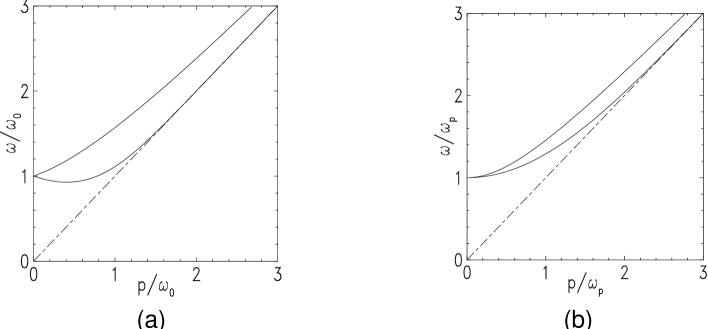
Figure 13: Dispersion relation for soft excitations in the linear regime: (a) soft fermions; the upper branch is the “normal” fermion, with dispersion relation $\omega_{+}(p)$, while the lower branch, with the characteristic plasmino minimum, is the “abnormal” mode, with energy $\omega_{-}(p)$; (b) soft gluons (or linear plasma waves), with the upper (lower) branch corresponding to transverse (longitudinal) polarization.

The dispersion relations for the modes are obtained from the poles of the propagators, that is,

$${p}^{2}+\Pi_{L}(\omega_{L},p)=0,\qquad\omega_{T}^{2}=p^{2}+\Pi_{T}(\omega_{T},p),$$ (4.40)

for longitudinal and transverse excitations, respectively. The solutions to these equations, $\omega_{L}(p)$ and $\omega_{T}(p)$, are displayed in fig. 13.b. The longitudinal mode is the analog of the familiar plasma oscillation. It corresponds to a collective oscillation of the hard particles, and disappears when $p\gg gT$. Both dispersion relations are time-like ($\omega_{L,T}(p)>p$), and show a gap at zero momentum (the same for transverse and longitudinal modes since, when $p\to 0$, we recover isotropy). As we shall see in Sect. 4.3.3, there is no Landau damping for the soft modes in the HTL approximation. Rather, these modes get attenuated via collisions in the plasma, a mechanism which matters at higher order in $g$ and which will be discussed in Sect. 6.

For small $p\ll m_{D}$, the dispersion relations read:

$$\omega_{T}^{2}\,=\,\omega_{pl}^{2}+{3\over 5}\,p^{2}+\cdots\qquad\qquad\omega_{L}^{2}\,=\,\omega_{pl}^{2}+{6\over 5}\,p^{2}+\cdots$$ (4.41)

where $\omega_{pl}\equiv m_{D}/{\sqrt{3}}$ is the plasma frequency (the gap in fig. 13.b). For large momenta, $p\gg m_{D}$, one has

$$\omega^{2}_{T}\,\simeq\,p^{2}+m_{D}^{2}/2,\qquad\qquad\omega^{2}_{L}\,\simeq\,p^{2}(1+4x_{L}),$$ (4.42)

where $x_{L}\equiv\exp\left\{-(2p^{2}/m_{D}^{2})-2\right\}.$ Thus, with increasing momentum, the transverse branch becomes that of a relativistic particle with an effective mass $m_{\infty}\equiv m_{D}/\sqrt{2}$ (commonly referred to as the “asymptotic mass”). Although, strictly speaking, the HTL approximation does not apply at hard momenta, the above dispersion relation $\omega_{T}(p)$ remains nevertheless correct for $p\sim T$ where it coincides with the light-cone limit of the full one-loop result [151] :

$$m_{\infty}^{2}\,\equiv\,\Pi_{T}^{1-loop}(\omega^{2}=p^{2})\,=\,{m_{D}^{2}\over 2}.$$ (4.43)

The longitudinal branch, on the other hand, approaches the light cone exponentially, but, as already mentioned, it disappears from the spectrum, as its residue is exponentially suppressed [149].

We turn now to soft fermionic excitations. The corresponding HTL is easily obtained from eq. (4.18) with $A^{\mu}\to 0$, and reads (cf. Sect. 5.3.1) :

$$\Sigma(\omega,{\bf p})\,=\,\omega_{0}^{2}\int{{\rm d}\Omega\over 4\pi}{\hbox to0.0pt{\hbox to5.20601pt{\hfil/\hfil}\hss}v\over\omega-{\bf v}\cdot{\bf p}+i\eta}\,.$$ (4.44)

Let us first consider in more detail what happens in the long wavelength limit, $p\to 0$. From eq. (4.44) one gets then:

$$\Sigma(\omega,p=0)\,=\,{\omega_{0}^{2}\over\omega}\,\gamma_{0}.$$ (4.45)

The spectrum at $p=0$ is thus obtained from the poles of

$${}^{*}\!S(\omega)\,=\,{\gamma_{0}\over-\omega+\omega_{0}^{2}/\omega}\,.$$ (4.46)

For each eigenstate of $\gamma_{0}$, corresponding to the eigenvalues $\pm 1$, there are two poles, at $\omega=\pm\omega_{0}$. Thus, the pole at $\omega=\omega_{0}$ is double degenerate, and similarly for the pole at $\omega=-\omega_{0}$. This degeneracy is removed by a small (zero-temperature) mass, or, as we shall see, by a finite momentum $p$, which leads to the split spectrum shown in fig. 13.a.

Consider then the HTL-resummed propagator ${}^{*}\!S$ at finite momentum. This has the following structure (cf. Sect. B.2.3):

$${}^{*}\!S(\omega,{\bf p})\gamma_{0}\,=\,{}^{*}\!\Delta_{+}(\omega,p)\Lambda_{+}(\hat{\bf p})\,+\,{}^{*}\!\Delta_{-}(\omega,p)\Lambda_{-}(\hat{\bf p})\,,$$ (4.47)

with the functions ${}^{*}\!\Delta_{\pm}$ given by eq. (B.104), and the matrices $\Lambda_{\pm}\equiv(1\pm\gamma^{0}\mbox{\boldmath$\gamma$}\cdot\hat{\bf p})/{2}$ are projectors. Charge conjugation exchanges the poles of ${}^{*}\!\Delta_{+}$ and ${}^{*}\!\Delta_{-}$. ${}^{*}\!\Delta_{+}$ has two poles, one at positive $\omega$, with energy $\omega_{+}(p)$, and another one at negative $\omega$, with energy $-\omega_{-}(p)$; these go over to $\pm\omega_{0}$ as $p\to 0$. Correspondingly, ${}^{*}\!\Delta_{-}$ has poles at $\omega_{-}$ and $-\omega_{+}$.

In the limit $p\gg\omega_{0}$, the branches $\pm\omega_{+}(p)$ describe the “normal” (anti)fermion, with a dispersion relation

$$\omega_{+}^{2}(p)\,\simeq\,p^{2}+M_{\infty}^{2}\,,\qquad M_{\infty}^{2}\,\equiv\,2\omega_{0}^{2}\,,$$ (4.48)

describing the propagation of a massive particle with the “asymptotic” mass $M_{\infty}=\sqrt{2}\omega_{0}$. In the same limit, the “abnormal” branches $\pm\omega_{-}(p)$ disappear from the spectrum since their residues are exponentially suppressed [150]. Incidentally, eq. (4.48) is also correct for $p\sim T$, where it coincides with the full one-loop result [151].

For generic soft momenta, on the other hand, all the four branches are present in the spectrum, and describe collective excitations in which the hard quarks get converted into hard gluons, or vice-versa, giving rise to longwavelength oscillations in the number density of the hard fermions. In particular, for $p\ll\omega_{0}$,

$$\omega_{+}(p)\,\simeq\,\omega_{0}\,+\,{p\over 3}\,+\cdots,\qquad\omega_{-}(p)\,\simeq\,\omega_{0}\,-\,{p\over 3}\,+\cdots,$$ (4.49)

so that the “abnormal” (or “plasmino”) branch is actually decreasing at small $p$, down to a minimum at $p=p_{min}\approx.408\,\omega_{0}\,$, and then it increases and approaches $\omega=p$, as shown in fig. 13.a. The origin of this peculiar behaviour is a collective phenomenon whereby the single particle strength at small momentum $p$ is split by the coupling of the soft modes to the hard particles which form a continuum of states with energy $|\omega|<p$. Due to this coupling, a fraction of the anti–fermion strength, initially at energy $\omega=-p$, is pushed up to the positive energy $\omega=\omega_{-}(p)$, producing the abnormal branch. For small $p$ the behaviour of $\omega_{-}(p)$ is therefore that of a negative energy state: it decreases as $p$ increases. This physical interpretation is made explicit by the construction of the plasmino state at zero temperature and large chemical potential in Ref. [152].

We note finally that particular solutions of the non-linear equations (4.2) have also been found, in Refs. [153, 154, 21]. These solutions describe non-linear plane-waves propagating through the plasma, and represent truly non-Abelian collective excitations.

4.3.2 Debye screening

The screening of a static chromoelectric field by the plasma constituents is the natural non-Abelian generalization of the Debye screening, a familiar phenomenon in classical plasma physics [43]. In coordinate space, screening means that the range of the gauge interactions is reduced as compared to the vacuum. In momentum space, this corresponds to a softening of the infrared behaviour of the various $n$-point functions.

Consider a static colour field, that is, a field configuration which, at least in some particular gauge, can be represented by time-independent gauge potentials $A^{a}_{\mu}({\bf x})$. For such fields, the expression (4.33) of the colour current reduces to its first, local, term (a static colour charge density):

$$j_{\mu}^{A\,a}({\bf x})\,=\,-\,\delta_{\mu 0}\,m^{2}_{D}A_{0}^{a}({\bf x})\,.$$ (4.50)

The equations of motion (4.2) simplify accordingly:

$$[D_{i},E^{i}({\bf x})]\,+\,m_{D}^{2}A^{0}({\bf x})\,=\,0,$$

$$\epsilon^{ijk}[D_{j},B^{k}]\,=\,i\,g\,[A^{0},E^{i}].$$ (4.51)

They differ from the corresponding equations in the vacuum only by the presence of a “mass” term $m_{D}^{2}\,A^{2}_{0}$ for the electrostatic fields.

To appreciate the role of this mass, consider first the Abelian case, where the equations above are linear:

$$(-\Delta\,+\,m^{2}_{D})\,A_{0}({\bf x}) = \rho({\bf x}),$$

$$\Delta A^{i}\,-\,\nabla^{i}(\mbox{\boldmath$\nabla$}\cdot{\bf A}) = 0.$$ (4.52)

The first equation, in which we have added an external source with charge density $\rho({\bf x})=Q\,\delta^{(3)}({\bf x})$, is easily solved by Fourier transform and yields the familiar screened Coulomb potential:

$$A_{0}(r)=Q\int{{\rm d}^{3}p\over(2\pi)^{3}}\,{{\rm e}^{i{\bf p}\cdot{\bf r}}\over p^{2}+m^{2}_{D}}\,=\,Q\,{{\rm e}^{-m_{D}r}\over 4\pi r}\,.$$ (4.53)

The second equation (4.3.2) shows that the static magnetic fields are not screened, which can be related to the fact that plasma particles carry no magnetic charges.

The same conclusion can be reached by an analysis of the effective photon (or gluon) propagators (4.38) in the static limit $\omega\to 0$. Eqs. (B.63) imply

$$\Pi_{L}(0,p)\,=\,m_{D}^{2}\,,\qquad\,\,\,\,\Pi_{T}(0,p)=0,$$ (4.54)

and therefore:

$${}^{*}\!\Delta_{L}(0,p)\,=\,{-1\over p^{2}+m_{D}^{2}}\,,\qquad{}^{*}\!\Delta_{T}(0,p)\,=\,{1\over p^{2}}\,,$$ (4.55)

which clearly shows that the Debye mass acts as an infrared cut-off $\sim gT$ in the electric sector, while there is no such cut-off in the magnetic sector.

In non-Abelian plasmas, Debye screening may be accompanied by interesting non-linear effects. A particular solution to eqs. (4.3.2) is [140]

$$A_{0}^{a}\,=\,{\cal A}\,\hat{r}^{a}\,{{\rm e}^{-m_{D}r}\over r}\,,\qquad\,\,A_{i}^{a}\,=\,\epsilon^{aij}\hat{r}^{j}\,{1\over r}\,,$$ (4.56)

where ${\cal A}$ is a constant and $\hat{r}^{i}=x^{i}/r$. This solution is a superposition of the Wu-Yang magnetic monopole [155] and a screened electrostatic field. More generally, it has been shown in Ref. [140] that all the ($SU(2)$-radially symmetric) solutions which are regular at infinity approach at the origin the monopole solution (4.56). That is, all such solutions show electric screening, but there is no sign of magnetic screening, in spite of the non-Abelian coupling between electric and magnetic fields in eqs. (4.3.2). Moreover, there are no finite energy solutions (no static solitons), in complete analogy to what happens in the vacuum (i.e., for $m_{D}=0$) [156].

4.3.3 Landau damping

For time-dependent fields, there exists a different screening mechanism associated to the energy transfer to the plasma constituents. In Abelian plasmas, this mechanism is known as Landau damping [43]. For simplicity, let us start with this Abelian case, and compute the mechanical work done by a longwavelength electromagnetic field acting on the charged particles. The rate of energy transfer has the familiar expression [43]:

$${{\rm d}\,{\rm E}_{W}(t)\over{\rm d}\,t}\,=\,\int{\rm d}^{3}{\bf x}\,{\bf E}(t,\,{\bf x})\cdot{\bf j}(t,\,{\bf x}),$$ (4.57)

where $j^{i}(p)=\Pi_{R}^{i\nu}(p)A_{\nu}(p)$ is the induced current. Consider, for instance, a periodic electric field of the form ${\bf E}(t,\,{{\bf p}})\,=\,{\bf E}({\bf p})\,\cos\omega_{0}t$. From eq. (4.57), one can compute the average energy loss over one period $T_{0}=2\pi/\omega_{0}$, with the following result:

$$\left\langle{{\rm d}\,{\rm E}_{W}\over{\rm d}\,t}\right\rangle = {1\over 2\omega_{0}}\int{{\rm d}^{3}p\over(2\pi)^{3}}\,E^{i}(-{\bf p})\left(-{\rm Im}\,\Pi_{R}^{ij}(\omega_{0},\,{\bf p})\right)\,E^{j}({\bf p})$$ (4.58)

$$= {\pi m_{D}^{2}\over 2}\int{{\rm d}\Omega\over 4\pi}\,\delta(\omega-{\bf v}\cdot{\bf p})\,\Big{|}{\bf v}\cdot{\bf E}({\bf p})\Big{|}^{2},$$

where we have used the following expression for the imaginary part of the retarded polarization tensor (cf. eq. (1.19))

$${\rm Im}\,\Pi_{R}^{\mu\nu}(\omega,{\bf p})\,=\,-\,\pi m_{D}^{2}\,\omega\int{{\rm d}\Omega\over 4\pi}\,\,v^{\mu}v^{\nu}\,\delta(\omega-{\bf v}\cdot{\bf p})\,.$$ (4.59)

The expression in eq. (4.58) is non-negative: on the average, the energy is transferred from the electromagnetic field to the particles. The $\delta$-function in Eq. (4.58) shows that the particles which absorb energy are those moving in phase with the field (i.e., the particles whose velocity component along ${\bf p}$ is equal to the field phase velocity: ${\bf v}\cdot\hat{\bf p}=\omega/p$). Since in ultrarelativistic plasmas ${\bf v}$ is a unit vector, only space-like ($|\omega|<p$) fields are damped in this way.

To see how this mechanism leads to screening, consider the effective photon (or gluon) propagator in the hard thermal loop approximation (cf. eq. (4.38)), and focus on the magnetic propagator. For small but non-vanishing frequencies the corresponding polarization function $\Pi_{T}(\omega,p)$ is dominated by its imaginary part, which vanishes linearly as $\omega\to 0$ (see eq. (4.59)), in contrast to the real part which vanishes quadratically. Specifically, the second equation (B.63) yields:

$$\Pi_{T}(\omega\ll p)\,=\,-i\,{\pi\over 4}\,m_{D}^{2}\,{\omega\over p}+\,{\rm O}(\omega^{2}/p^{2})\,,$$ (4.60)

and therefore

$${}^{*}\!\Delta_{T}(\omega\ll p)\simeq\,{1\over p^{2}-i\,(\pi\omega/4p)\,m_{D}^{2}}.$$ (4.61)

In the computation of scattering cross sections, the relevant matrix element squared is proportional to (see, e.g., eq. (6.3))

$$|{}^{*}\!\Delta_{T}(\omega,p)|^{2}\,\simeq\,{1\over p^{4}+(\pi m_{D}^{2}\omega/4p)^{2}}\,,$$ (4.62)

which shows that Im$\,\Pi_{T}(p)$ acts as a frequency-dependent IR cutoff at momenta $p\sim(\omega m_{D}^{2})^{1/3}$. That is, as long as the frequency $\omega$ is different from zero, the soft momenta are dynamically screened by Landau damping [63].

Dynamical screening occurs also for the longitudinal interactions, but in this case it is less important, since Debye screening dominates at small frequency.

Furthermore, in the case of QCD, the study of Landau damping is complicated by non-linear effects. The non-Abelian expression for the rate of mechanical work (see eq. (4.67) below) involves the non-linear colour current (4.16); accordingly, all the $n$-point HTL amplitudes (self-energy and vertices) develop imaginary parts (see Sect. 5). Moreover, the Landau damping is also operative for soft fermions, both in QCD and in QED; this is described, e.g., by the imaginary part of the fermion self-energy, eq. (4.44).

4.4 Hamiltonian theory for the HTL’s

There exists a concise and elegant formulation of the effective theory for the soft fields dynamics as a Hamiltonian theory [24, 75, 77]. At first sight, this may be surprising since the corresponding equation of motion, namely eq. (4.2), (the fermionic fields are set to zero in this section):

$$\left[\,D^{\nu},\,F_{\nu\mu}(x)\,\right]^{a}\,=\,m^{2}_{D}\int{{\rm d}\Omega\over 4\pi}\,v_{\mu}\int_{0}^{\infty}{\rm d}\tau\,U_{ab}(x,x-v\tau)\,{\bf v}\cdot{\bf E}^{b}(x-v\tau)\,,$$ (4.63)

is non-local in space and time, and also dissipative: Because of Landau damping, energy is transferred between the particles and the background fields. However, at the expense of keeping the field $W^{a}_{0}(x,{\bf v})$ as a soft degree of freedom (summarizing the effects of the plasma particles), one can rewrite eq. (4.63) as to the following system of local equations (cf. eqs. (4.7) and (4.12)):

$$\left[\,D^{\nu},\,F_{\nu\mu}(x)\,\right]^{a} = m^{2}_{D}\int{{\rm d}\Omega\over 4\pi}\,v_{\mu}\,W^{a}_{0}(x,{\bf v}),$$

$$\left[v\cdot D_{x},\,W_{0}(x,{\bf v})\right]^{a} = {\bf v\cdot E}^{a}(x).$$ (4.64)

The fields $A^{\mu}_{a}(x)$ and $W^{a}_{0}(x,{\bf v})$ will be regarded as independent degrees of freedom in the following.

4.4.1 The energy of the colour fields

In order to obtain the Hamilton function for these degrees of freedom, we start by computing the energy ${\rm E}$ carried by the longwavelength colour excitations [138, 139, 24, 75]. We can write:

$${\rm E}\,=\,{\rm E}_{YM}(t)\,+\,{\rm E}_{W}(t)\,\equiv\,\int{\rm d}^{3}{\bf x}\,{\cal E}(t,\,{\bf x}),$$ (4.65)

where ${\rm E}_{YM}(t)$ is the energy stored in the colour fields at time $t$,

$${\rm E}_{YM}(t)\,=\,\int{\rm d}^{3}{\bf x}\,{1\over 2}\Bigl{(}{\bf E}^{a}(t,\,{\bf x})\cdot{\bf E}^{a}(t,\,{\bf x})\,+\,{\bf B}^{a}(t,\,{\bf x})\cdot{\bf B}^{a}(t,\,{\bf x})\Bigr{)},$$ (4.66)

while ${\rm E}_{W}(t)$ is the polarization energy, that is, the energy transferred by the colour field to the plasma constituents, as mechanical work. Energy conservation d${\rm E}/{\rm d}t=0$, together with the first equation (4.4), imply

$${{\rm d}\,{\rm E}_{W}(t)\over{\rm d}\,t}\,=\,\int{\rm d}^{3}{\bf x}\,{\bf E}^{a}(t,\,{\bf x})\cdot{\bf j}_{a}(t,\,{\bf x}),$$ (4.67)

where ${\bf j}_{a}$ is the induced current (4.12):

$${\bf j}_{a}(t,\,{\bf x})\,=\,m^{2}_{D}\int{{\rm d}\Omega\over 4\pi}\,{\bf v}\,W^{a}_{0}(x,{\bf v}).$$ (4.68)

We recognize in eq. (4.67) the non-Abelian generalization of eq. (4.58). By using the equation of motion for $W^{a}_{0}(x,{\bf v})$ (i.e. the second equation (4.4)), we can write:

$${\rm E}_{W}(t) = \int_{-\infty}^{t}dt^{\prime}\,\int{\rm d}^{3}{\bf x}^{\prime}\,{\bf E}^{a}(t^{\prime},\,{\bf x^{\prime}})\cdot{\bf j}_{a}(t^{\prime},\,{\bf x^{\prime}})$$ (4.69)

$$= m^{2}_{D}\int{{\rm d}\Omega\over 4\pi}\int_{-\infty}^{t}dt^{\prime}\,\int{\rm d}^{3}{\bf x}^{\prime}\,\,W^{a}_{0}(t^{\prime},\,{\bf x^{\prime}},{\bf v})\left[v\cdot D_{x^{\prime}},\,W_{0}(t^{\prime},\,{\bf x^{\prime}},{\bf v})\right]^{a}$$

$$= {m^{2}_{D}\over 2}\int{{\rm d}\Omega\over 4\pi}\int_{-\infty}^{t}dt^{\prime}\,\int{\rm d}^{3}{\bf x}^{\prime}\,(v\cdot\partial_{x^{\prime}})\left(W^{a}_{0}\,W_{0}^{a}\right).$$

The integral over $t^{\prime}$ can now be done (we assume the fields to vanish at spatial infinity and at $t\to-\infty$), and yields:

$${\rm E}_{W}(t)\,=\,{m^{2}_{D}\over 2}\int{\rm d}^{3}{\bf x}\int{{\rm d}\Omega\over 4\pi}\,\,W_{a}^{0}(x,{\bf v})\,W_{a}^{0}(x,{\bf v}).$$ (4.70)

Together, eqs. (4.65), (4.66) and (4.70) express the energy associated with the propagation of a longwavelength colour wave in a hot QCD plasma [75]. Clearly, this quantity is positive definite, which reflects the stability of the plasma with respect to longwavelength colour oscillations [24].

The energy flux density, or Poynting vector, of the propagating colour waves can be computed similarly, with the result [75]

$${\bf S}(x)\,=\,{\bf E}^{a}(x)\times{\bf B}^{a}(x)\,+\,{m_{D}^{2}\over 2}\int{d\Omega\over 4\pi}\,{\bf v}\,W_{a}^{0}(x,{\bf v})\,W_{a}^{0}(x,{\bf v}).$$ (4.71)

Then, the energy conservation can be also written in local form, as

$$\partial_{0}\,{\cal E}(x)\,+\,\partial_{i}\,S^{i}(x)\,=\,0,$$ (4.72)

where ${\cal E}(x)$ is the energy density in eq. (4.65). Note, however, that the above expressions are local only when expressed in terms of both the gauge fields $A^{\mu}_{a}(x)$ and the auxiliary fields $W^{0}_{a}(x,{\bf v})$.

4.4.2 Hamiltonian analysis

In the temporal gauge $A^{a}_{0}=0$, eqs. (4.4) become (with $W_{0}^{a}(x,{\bf v})\equiv W^{a}(x,{\bf v})$ in what follows)

$$\partial_{0}A^{a}_{i} = -E^{a}_{i},$$

$$-\partial_{0}E^{a}_{i}+\epsilon_{ijk}(D_{j}B_{k})^{a} = m_{D}^{2}\int{{\rm d}\Omega\over 4\pi}\,v_{i}\,W^{a}(x,{\bf v}),$$

$$\left(\partial_{0}+{\bf v\cdot D}\right)^{ab}W_{b} = {\bf v\cdot E}^{a},$$ (4.73)

together with Gauss’ law (the $\mu=0$ component of the first equation (4.4)):

$$G^{a}({\bf x})\equiv({\bf D\cdot E})^{a}\,+\,m_{D}^{2}\int{{\rm d}\Omega\over 4\pi}\,W^{a}(x,{\bf v})\,=\,0.$$ (4.74)

This last equation contains no time derivative and should therefore be regarded as a constraint.

We show now that eqs. (4.4.2) can be given a Hamiltonian structure. To this aim, consider the conserved energy in eq. (4.65) which we denote here by $H$:

$$H\,=\,{1\over 2}\int{\rm d}^{3}{\bf x}\left\{{\bf E}^{a}\cdot{\bf E}^{a}\,+\,{\bf B}^{a}\cdot{\bf B}^{a}\,+\,m_{D}^{2}\int{{\rm d}\Omega\over 4\pi}\,W^{a}(x,{\bf v})\,W^{a}(x,{\bf v})\right\}.$$ (4.75)

This expression is independent of the choice of gauge. However, in the gauge $A_{0}^{a}=0$, we can make it act as a Hamiltonian, that is, as the generator of the time evolution. As independent degrees of freedom, we choose the vector potentials $A^{i}_{a}({\bf x})$, the electric fields $E_{a}^{i}({\bf x})$, and the density matrices $W^{a}({\bf x,v})$. (Note that the latter are fields on the extended configuration space $E^{3}\times S^{2}$, with $E^{3}$ being the ordinary three-dimensional coordinate space and $S^{2}$ the unit sphere spanned by ${\bf v}$.) Then, following Nair [24], we organize this as a Hamiltonian system by introducing the following Poisson brackets:

$$\left\{E^{a}_{i}({\bf x}),A^{b}_{j}({\bf y})\right\} = -\,\delta^{ab}\delta_{ij}\delta^{(3)}({\bf x-y})\,,$$

$$\left\{E^{a}_{i}({\bf x}),W^{b}({\bf y,v})\right\} = v_{i}\,\delta^{ab}\delta^{(3)}({\bf x-y})\,,$$

$$m^{2}_{D}\left\{W^{a}({\bf x,v}),W^{b}({\bf y,v^{\prime}})\right\} = \left(gf^{abc}W^{c}+({\bf v\cdot D}_{x})^{ab}\right)\delta^{(3)}({\bf x-y})\delta({\bf v},{\bf v}^{\prime})\,.$$ (4.76)

Here, $\delta({\bf v},{\bf v}^{\prime})$ is the delta function on the unit sphere, normalized such that

$$\int{{\rm d}\Omega\over 4\pi}\,\delta({\bf v},{\bf v}^{\prime})\,f({\bf v})\,=\,f({\bf v}^{\prime}),$$ (4.77)

and all other brackets are assumed to vanish. We also assume the standard properties for the Poisson brackets, namely antisymmetry, bilinearity and Leibniz identity: $\{AB,C\}=A\{B,C\}+\{A,C\}B$. It is then straightforward to verify that (a) the Poisson brackets (4.4.2) satisfy the Jacobi identity (a necessary consistency condition) and (b) the equations of motion (4.4.2) follow as canonical equations for the Hamiltonian (4.75). For instance, $\partial_{0}W^{a}=\{H,W^{a}\}$, and similarly for $E_{i}^{a}$ and $A_{i}^{a}$.

The Hamiltonian in eq. (4.75) is remarkably simple: it is quadratic in the auxiliary fields $W^{a}_{0}$. Up to the colour indices, this piece would be the same in QED. Thus, all the non-Abelian complications are encoded in the Yang-Mills piece of $H$ and in the non-trivial Poisson brackets (4.4.2).

4.4.3 Effective classical thermal field theory

We shall now use the above Hamiltonian formulation of the HTL effective theory to write down a generating functional for the thermal correlations of the soft fields, in the classical approximation. As emphasized in Sect. 2.2.5, the classical approximation is correct only at soft momenta, so we shall introduce an ultraviolet cutoff $\Lambda$, with $gT\ll\Lambda\ll T$, to eliminate the hard ($k\mathrel{\hbox to0.0pt{\raise 2.20013pt\hbox{$>$}\hss}{\lower 2.20013pt\hbox{$\sim$}}}T$) fluctuations from the classical theory. Correspondingly, $\Lambda$ will act as an infrared cutoff for the hard, quantum, modes (see below).

We denote by ${\cal E}^{a}_{i}({\bf x})$, ${\cal A}^{a}_{i}({\bf x})$ and ${\cal W}^{a}({\bf x,v})$ the initial conditions for the HTL equations of motion (4.4.2). The partition function reads as follows (compare with eq. (2.130)):

$$Z_{cl}\,=\,\int{\cal D}{\cal E}^{a}_{i}\,{\cal D}{\cal A}^{a}_{i}\,{\cal D}{\cal W}^{a}\,\delta({\cal G}^{a})\,{\rm e}^{-\beta{\cal H}},$$ (4.78)

where ${\cal G}^{a}$ and ${\cal H}$ are expressed in terms of the initial fields as in eqs. (4.74) and (4.75). Eq. (4.78) can be rewritten as

$$Z_{cl}\,=\,\int{\cal D}{\cal A}^{a}_{0}\,{\cal D}{\cal A}^{a}_{i}\,\exp\left\{-{\beta\over 2}\int{\rm d}^{3}x\,\Bigl{(}{\cal B}^{a}_{i}{\cal B}^{a}_{i}+(D_{i}{\cal A}_{0})^{a}(D_{i}{\cal A}_{0})^{a}+m_{D}^{2}{\cal A}_{0}^{a}{\cal A}_{0}^{a}\Bigr{)}\right\},$$ (4.79)

where the temporal components ${\cal A}_{0}^{a}$ of the gauge fields have been reintroduced as Lagrange multipliers to enforce Gauss’ law, and the Gaussian functional integrals over ${\cal E}^{a}_{i}$ and ${\cal W}^{a}$ have been explicitly performed. In particular, the integral over the ${\cal W}^{\prime}$s has generated the screening mass for the electrostatic fields, as expected. We recognize in eq. (4.79) the static limit (5.19) of the HTL action.

More generally, time-dependent correlations of the soft fields are obtained by averaging products of fields $A^{i}_{a}(t,{\bf x})$ obeying eqs. (4.4.2). These correlations can be generated from

$$Z_{cl}[J^{a}_{i}]\,=\,\int{\cal D}{\cal E}^{a}_{i}\,{\cal D}{\cal A}^{a}_{i}\,{\cal D}{\cal W}^{a}\,\delta({\cal G}^{a})\,\exp\left\{-\beta{\cal H}\,+\,\int{\rm d}^{4}xJ^{a}_{i}(x)A^{a}_{i}(x)\right\},$$ (4.80)

where $A^{i}_{a}(t,{\bf x})$ is the solution to eqs. (4.4.2) (in particular, $A^{a}_{i}(t_{0},{\bf x})={\cal A}^{a}_{i}({\bf x})$), and the external current $J^{a}_{i}$ is introduced as a device to generate the correlations of interest via functional differentiations, but does not enter the equations of motion for the fields. It can be verified [77] that the phase-space measure ${\cal D}{\cal E}^{a}_{i}{\cal D}{\cal A}^{a}_{i}{\cal D}{\cal W}^{a}$ is invariant under the time evolution described by eqs. (4.4.2), so that $Z_{cl}[J]$ is independent of the initial time $t_{0}$, as it should. Since the dynamics is also gauge-invariant, it is sufficient to enforce Gauss’ law at $t=t_{0}$, as we did in eq. (4.80).

As a simple, but still non-trivial, check of eq. (4.80), let us consider the Abelian limit, where the equations of motion can be solved analytically, and the functional integral in eq. (4.80) can be computed exactly, since Gaussian [77]. We know already the result that we want to obtain: This should read (compare with eq. (2.133)) :

$$Z_{cl}[J_{i}] = Z_{cl}[0]\,\exp\left\{-{1\over 2}\int{\rm d}^{4}x\int{\rm d}^{4}y\,J^{i}(x)\,G_{ij}^{cl}(x-y)J^{j}(y)\right\},$$ (4.81)

$$G_{ij}^{cl}(x-y) \equiv \int{{\rm d}^{4}k\over(2\pi)^{4}}\,{\rm e}^{-ik\cdot(x-y)}\,\,{}^{*}\!\rho_{ij}(k)N_{cl}(k_{0}),$$ (4.82)

where $N_{cl}(k_{0})=T/k_{0}$, and ${}^{*}\!\rho_{ij}(p)$ is the photon spectral density in the HTL approximation and in the temporal gauge (cf. eqs. (B.68)–(B.71)) :

$${}^{*}\!\rho_{ij}(\omega,{\bf k})=(\delta_{ij}-\hat{k}_{i}\hat{k}_{j})\,{}^{*}\!\rho_{T}(\omega,k)\,+\,{k_{i}k_{j}\over\omega^{2}}\,\,{}^{*}\!\rho_{L}(\omega,k)\,.$$ (4.83)

The 2-point function (4.82) is the classical limit of the corresponding quantum correlator, which reads

$${}^{*}\!G_{\mu\nu}(x,y)=\int{{\rm d}^{4}k\over(2\pi)^{4}}\,{\rm e}^{-ik\cdot(x-y)}\,\,{}^{*}\!\rho_{\mu\nu}(k)\Bigl{[}\theta(x_{0}-y_{0})+N(k_{0})\Bigr{]}\,.$$ (4.84)

In the classical limit $N(k_{0})\approx T/k_{0}\gg 1$, so that the 2-point functions $G^{>}$ and $G^{<}$ reduce to the unique classical correlator $G^{cl}$ (see sections 2.1.4 and 2.2.5). For instance, in the transverse sector,

$${}^{*}\!G^{>}_{T}(\omega,k)\,\simeq\,{}^{*}\!G^{<}_{T}(\omega,k)\,\simeq\,{T\over\omega}\,\,{}^{*}\!\rho_{T}(\omega,k)\,=\,G_{T}^{cl}(\omega,k).$$ (4.85)

It is our purpose here to verify that eqs. (4.81)–(4.83) emerge indeed from the computation of the Abelian version of the functional integral (4.80).

To this aim, we have to solve first the linearized equations of motion (4.4.2) :

$$\Bigl{[}(\partial_{0}^{2}-\mbox{\boldmath$\nabla$}^{2})\delta^{ij}+\partial^{i}\partial^{j}\Bigr{]}A^{j}(x) = m_{D}^{2}\int{{\rm d}\Omega\over 4\pi}\,v^{i}\,W(x,{\bf v}),$$

$$\left(\partial_{0}+{\bf v}\cdot\mbox{\boldmath$\nabla$}\right)W(x,{\bf v}) = {\bf v\cdot E}(x),$$ (4.86)

with the initial conditions

$$A^{i}(t_{0},{\bf x})={\cal A}^{i}({\bf x}),\qquad\dot{A}^{i}(t_{0},{\bf x})=-{\cal E}^{i}({\bf x}),\qquad W(t_{0},{\bf x,v})={\cal W}({\bf x,v}).$$ (4.87)

To simplify the presentation we shall limit ourselves here to the transverse sector, and consider the transverse projection of the first equation (4.4.3),

$$(\partial_{0}^{2}+{\bf k}^{2})A^{i}_{T}\,=\,m_{D}^{2}\int{{\rm d}\Omega\over 4\pi}\,v_{T}^{i}\,W({\bf k,v}),$$ (4.88)

with ${\bf k\cdot A}_{T}=0$ and $v_{T}^{i}=(\delta^{ij}-\hat{k}^{i}\hat{k}^{j})v^{j}$. We choose as initial conditions ${\cal A}_{T}^{i}=0$ and ${\cal E}^{i}_{T}=0$, but let ${\cal W}({\bf x,v})$ be arbitrary. That is, for the gauge fields, we choose as initial values the corresponding average values in thermal equilibrium. All the fluctuations are generated by the randomly chosen initial conditions for $W({\bf x,v})$, that is, by the longwavelength initial fluctuations in the charge density of the hard fermions. These fluctuations will generate time-dependent gauge fields, via the equations of motion (4.4.3).

Consider then the solution $W(x,{\bf v})$ to the Vlasov equation (i.e., the second equation (4.4.3)) which we write as:

$$W\,=\,W_{ind}+W_{fl},$$ (4.89)

where $W_{ind}$ is the solution to the Vlasov equation with zero initial condition: $W_{ind}(t_{0},{\bf x,v})=0$), and $W_{fl}$ is the fluctuating piece, solution of the homogeneous equation

$$\left(\partial_{0}+{\bf v}\cdot\mbox{\boldmath$\nabla$}\right)W_{fl} = 0,$$ (4.90)

with the initial condition $W_{fl}(t_{0},{\bf x,v})={\cal W}({\bf x,v})$. It follows that (for $x_{0}>t_{0}$):

$$W_{ind}(x,{\bf v}) = -i\int{\rm d}^{4}y\,\theta(y_{0}-t_{0})\,G_{R}(x,y|{\bf v})\,\,{\bf v\cdot E}(y),$$

$$W_{fl}(x,{\bf v}) = {\cal W}({\bf x-v}(x_{0}-t_{0}),{\bf v}),$$ (4.91)

where $G_{R}(x,y|{\bf v})$ is the retarded Green’s function in eq. (4.2). Eq. (4.89) implies a similar decomposition for the current: $j^{i}=j^{i}_{ind}+\xi^{i}$, with

$$j^{i}_{ind}(x) = -\int{\rm d}^{4}y\,\theta(y_{0}-t_{0})\,\Pi_{R}^{ij}(x-y)A^{j}(y)$$

$$\xi^{i}(x) = m_{D}^{2}\int{{\rm d}\Omega\over 4\pi}\,v^{i}\,{\cal W}({\bf x-v}(x_{0}-t_{0}),{\bf v}),$$ (4.92)

where $\Pi_{R}^{ij}$ is the (retarded) HTL polarization tensor given in eq. (1.19).

The Maxwell equation (4.88) now becomes

$$(\partial_{0}^{2}+{\bf k}^{2})A^{i}_{T}\,+\,\int_{t_{0}}^{\infty}{\rm d}y_{0}\,\Pi_{T}(x_{0}-y_{0},{\bf k})A^{i}_{T}(y_{0})=\xi_{T}^{i},$$ (4.93)

which should be compared with the equation that we had before, namely the first equation (4.2): the crucial difference is the presence of the fluctuating current $\xi^{i}(x)$ in the right hand side, which is independent of the gauge fields, and acts as a “noise term” to induce the thermal correlations of the classical electromagnetic fields. Specifically, eqs. (4.78) and (4.75) imply that the initial conditions ${\cal W}$ are Gaussian random variables with zero expectation value and the following, local, 2-point correlation:

$$\langle{\cal W}({\bf x,v})\,{\cal W}({\bf y,v}^{\prime})\rangle=(T/m^{2}_{D})\,\delta^{(3)}({\bf x-y})\delta({\bf v},{\bf v}^{\prime}).$$ (4.94)

This immediately implies:

$$\langle\xi^{i}(x)\xi^{j}(y)\rangle\,=\,m^{2}_{D}T\int{{\rm d}\Omega\over 4\pi}v^{i}v^{j}\delta^{(3)}({\bf x-y}-{\bf v}(x_{0}-y_{0})),$$ (4.95)

which is non-local; that is, the fluctuating current $\xi^{i}(x)$ is not a “white noise”. For $t_{0}\to-\infty$, eq. (4.93) can be easily solved by Fourier transform to yield (recall that ${\cal A}_{T}^{i}={\cal E}_{T}^{i}=0$):

$$A_{T}^{i}(k)\,=\,\,{}^{*}\!\Delta_{T}(k)\,\xi_{T}^{i}(k),$$ (4.96)

where ${}^{*}\!\Delta_{T}(k)$ is the retarded magnetic propagator in the HTL approximation, cf. eq. (4.38). The gauge field correlation induced by the “noise term” $\xi^{i}(x)$ is finally obtained as:

$$\langle A_{T}^{i}(k)A_{T}^{j\,*}(p)\rangle\,=\,(2\pi)^{4}\delta^{(4)}(p+k)\,(\delta^{ij}-\hat{k}^{i}\hat{k}^{j})\,\tilde{G}_{T}^{cl}(k),$$ (4.97)

with

$$\tilde{G}_{T}^{cl}(\omega,k) \equiv m^{2}_{D}T\,|{}^{*}\!\Delta_{T}(k)|^{2}\,\int{{\rm d}\Omega\over 4\pi}\,\,{\bf v}_{T}^{2}\,\,2\pi\,\delta(\omega-{\bf v\cdot k})$$ (4.98)

$$= -2\,(T/\omega)\,|{}^{*}\!\Delta_{T}(k)|^{2}\,\,{\rm Im}\,\Pi_{T}(\omega,k),$$

where in writing the second line we have recognized ${\rm Im}\,\Pi_{T}$ from eq. (4.59). This can be rewritten as

$$\tilde{G}_{T}^{cl}(\omega,k)\,=\,(T/\omega)\,\beta_{T}(\omega,k),$$ (4.99)

where $\beta_{T}$ is the off-shell (or Landau damping) piece of the transverse photon spectral density in the HTL approximation (cf. eqs. (B.71) and (B.1.3) in the Appendix).

Thus, by averaging over the initial conditions ${\cal W}$ alone, one has generated the Landau damping piece of the magnetic propagator. Similarly, by averaging over the initial fields ${\cal A}_{T}^{i}$ and ${\cal E}_{T}^{i}$, one generates also the pole piece, ${}^{*}\!\rho_{T}^{\,pole}\propto\delta(\omega^{2}-\omega_{T}^{2}(k))$ [77]. Altogether, this gives the classical transverse 2-point function in the expected form (cf. eq. (4.85)):

$$G_{T}^{cl}(\omega,k)\,=\,(T/\omega)\,\,{}^{*}\!\rho_{T}(\omega,k).$$ (4.100)

An entirely similar result holds for the longitudinal 2-point function as well [77], which completes the verification of the result announced in eqs. (4.81)–(4.83). One thus sees, on the example of the 2-point function in QED, that the physics of HTL’s is correctly reproduced by the classical theory.

We note that in this calculation the intermediate scale $\Lambda$ did not play any role. In QCD, however, because the equations of motion for the soft modes are non-linear, the average over the initial conditions generate soft thermal loops which are linearly ultraviolet divergent (as for the scalar theory in Sect. 2.1.4; recall, especially, eq. (2.80) there). In this case, the intermediate scale $\Lambda$, with $gT\ll\Lambda\ll T$, is necessary. As compared with the classical theory in Sect. 2.2.5, the new complication here is that the cutoff procedure must be implemented in a way consistent with gauge symmetry. Furthermore, in numerical solutions of the equations of motion using the lattice techniques, an additional complication arises from the fact that the lattice regularization breaks rotational and dilation symmetries. As a consequence, the ultraviolet divergences of the lattice theory cannot be all absorbed into just one parameter, a “lattice Debye mass”. In spite of many efforts [74, 83, 77, 84], no complete solution to such problems has been found.

Nevertheless, the HTL effective theory has been already implemented on a lattice [27] (see also Refs. [57, 28, 157]), and applied to the calculation of the anomalous baryon number violation rate in a high-temperature Yang-Mills theory (cf. Sect. 1.6). Remarkably, the results obtained in this way, even without any matching, appear to be rather insensitive to lattice artifacts, and are moreover consistent with some previous numerical calculations [57] (where the HTL’s are simulated via classical coloured “test particles” [54]), and also with the theoretical predictions in Refs. [78, 25].

5 Hard thermal loops

In the previous section we have obtained explicit expressions for the induced sources as functionals of the mean fields. These functionals may be used to obtain, by successive differentiations with respect to the fields, the effective propagators and vertices for the soft fields. The resulting expressions are the so-called “hard thermal loops” (HTL) [42, 19, 20, 22], i.e., the leading order thermal corrections to the one-particle-irreducible (1P-I) amplitudes with soft external lines.

These amplitudes may be used as building blocks to improve perturbative calculations through various resummation schemes. These will be discussed in the last section of this chapter, which contains also digressions on the limitation of weak coupling calculations and how these can be overcome using lattice calculations.

5.1 Irreducible amplitudes from induced sources

By taking the derivatives of the effective action $\Gamma\bigl{[}A,\Psi,\bar{\Psi}\bigr{]}$ with respect to its field arguments, we obtain the equations of motion for the mean fields (all the subsequent formulae hold for time arguments along a complex contour of the type discussed in Sect. 2) :

$$j^{\mu}=-{\delta\Gamma\over\delta A_{\mu}},\qquad\eta=-{\delta\Gamma\over\delta\bar{\Psi}},\qquad\bar{\eta}={\delta\Gamma\over\delta\Psi},$$ (5.1)

where $j^{\mu},\eta,\bar{\eta}$ are external sources. By writing $\Gamma=S_{cl}+\Gamma_{ind}$, where $S_{cl}$ is the classical action (A.11), we get:

$$j_{a}^{\mu}(x) = \left[\,D_{\nu},\,F^{\nu\mu}(x)\,\right]^{a}-g\bar{\Psi}(x)\gamma^{\mu}t^{a}\Psi(x)\,-\,{\delta\Gamma_{ind}\over\delta A_{\mu}^{a}(x)},$$

$$\eta(x) = i\hbox to0.0pt{\hbox to8.55695pt{\hfil/\hfil}\hss}D\,\Psi(x)\,-\,{\delta\Gamma_{ind}\over\delta\bar{\Psi}(x)}.$$ (5.2)

Then, a comparison with eqs. (3.45)–(3.46) allows us to identify the induced sources as the first derivatives of $\Gamma_{ind}\,$:

$$j^{ind}_{\mu\,a}(x)={\delta\Gamma_{ind}\over\delta A^{\mu}_{a}(x)},\qquad\eta^{ind}(x)={\delta\Gamma_{ind}\over\delta\bar{\Psi}(x)},\qquad\bar{\eta}^{ind}(x)=-{\delta\Gamma_{ind}\over\delta\Psi(x)}.$$ (5.3)

Accordingly, all the $n$-point 1P-I Green’s functions with $n\geq 2$ can be obtained by differentiating the induced sources with respect to the mean fields. Unless otherwise specified, we set the fields to zero after differentiation. That is, we compute the equilibrium 1P-I Green’s functions.

For instance, the gluon 1P-I 2-point function (which coincides with the gluon inverse propagator) is obtained as

$$(D^{-1})_{\mu\nu}^{ab}(x,y)\,=\,{\delta^{2}\Gamma\over\delta A^{\mu}_{a}(x)\delta A^{\nu}_{b}(y)}\,=\,(D_{0}^{-1})_{\mu\nu}^{ab}(x,y)+\Pi_{\mu\nu}^{ab}(x,y),$$ (5.4)

where:

$$(D_{0}^{-1})_{\mu\nu}^{ab}(x,y)\,=\,\delta^{ab}\left(-g_{\mu\nu}\partial^{2}+(1-\lambda^{-1})\partial_{\mu}\partial_{\nu}\right)\delta_{C}(x-y)$$ (5.5)

is the corresponding free propagator written here in a covariant gauge with gauge fixing term $(\partial\cdot A^{a})^{2}/2\lambda$, and

$$\Pi_{\mu\nu}^{ab}(x,y)={\delta j_{\mu}^{ind\,a}(x)\over\delta A_{b}^{\nu}(y)}$$ (5.6)

is the gluon polarization tensor. For fermions we write similarly:

$$S^{-1}(x,y)\,=\,{\delta^{2}\Gamma\over\delta\Psi(y)\delta\bar{\Psi}(x)}\,=\,S_{0}^{-1}+\Sigma,$$ (5.7)

with the free propagator $S_{0}^{-1}(x,y)=-i{\hbox to0.0pt{\hbox to5.30904pt{\hfil/\hfil}\hss}\partial}_{x}\,\delta(x-y)$ and the self-energy

$$\Sigma(x,y)={\delta\eta^{ind}(x)\over\delta\Psi(y)}\,.$$ (5.8)

More differentiations yield the irreducible (or proper) vertices. For instance, the quark-gluon vertex is

$${\delta^{3}\Gamma\over\delta\Psi(z)\delta\bar{\Psi}(y)\delta A_{\mu}^{a}(x)}=g\gamma^{\mu}t^{a}\delta_{C}(x-y)\delta_{C}(y-z)+g\Gamma_{a}^{\mu}(x,y,z),$$ (5.9)

whose induced part is obtained either from the induced color current $j^{ind}_{\mu}$, or from the fermionic source $\eta^{ind}$, according to

$$g\Gamma^{a}_{\mu}(x,y,z)={\delta^{2}j^{ind}_{\mu\,a}(x)\over\delta\Psi(z)\delta\bar{\Psi}(y)}={\delta^{2}\eta^{ind}(y)\over\delta A_{\mu}^{a}(x)\delta\Psi(z)}\,.$$ (5.10)

Similarly, the proper three-gluon vertex is obtained as

$$g\Gamma_{\mu\nu\rho}^{abc}(x,y,z)={\delta^{2}j_{\mu}^{ind\,a}(x)\over\delta A_{b}^{\nu}(y)\delta A_{c}^{\rho}(z)}\,.$$ (5.11)

The induced piece $\Gamma_{ind}$ of the effective action depends in general on the specific form of the gauge fixing term $G^{a}[A]$ in the generating functional (3.16), and, within a given class of gauges (i.e. for a given $G^{a}[A]$), on the gauge parameter $\lambda$. Moreover, as a functional of the classical fields $A^{\mu}_{a}$, $\Psi$ and $\bar{\Psi}$, $\Gamma_{ind}$ is generally not invariant under the gauge transformations of its arguments.

However, in the HTL approximation, the induced sources are both independent of the quantum gauge fixing, and also covariant under the gauge transformations of the classical fields. Besides, the induced current is covariantly conserved, $[D^{\mu},j^{ind}_{\mu}]=0$, cf. eqs. (4.14) and (4.21). Together, these conditions guarantee that the HTL effective action (to be denoted as $\Gamma_{HTL}$) is both gauge-fixing independent, and invariant under the gauge transformations of its field arguments. The latter property can be easily verified as follows: Under the infinitesimal gauge transformation (we omit the fermionic fields, for simplicity)

$$A_{\nu}\rightarrow A_{\nu}+\delta A_{\nu},\qquad\delta A_{\nu}\,=\,-\,{1\over g}\,[D_{\nu},\theta],$$ (5.12)

the induced action changes as (cf. eq. (5.3))

$$\delta\Gamma_{ind}=\int_{C}{\rm d}^{4}x\,j^{ind}_{\nu\,a}\delta A_{a}^{\nu}\,=\,-\int_{C}{\rm d}^{4}x\,[D^{\nu},\,j^{ind}_{\nu}]_{a},$$ (5.13)

where the second equality follows after an integration by parts (the surface term has been assumed to vanish). Clearly, the gauge invariance of $\Gamma_{ind}$ requires that $j^{ind}_{\nu}$ is covariantly conserved, a condition satisfied indeed at the HTL level, i.e. for $\Gamma_{ind}=\Gamma_{HTL}$.

5.2 The HTL effective action

Since the induced sources are known explicitly in terms of the classical fields $A^{\mu}_{a}$, $\Psi$ and $\bar{\Psi}$, it is tempting to try and use eq. (5.3) to construct also the effective action in explicit form. Note, however, that the induced sources are known only for real-time arguments, and for retarded (or advanced) boundary conditions (cf. Sect. 4.1). Thus, the contour action cannot be derived by simply integrating eqs. (5.3) with the induced sources in Sect. 4.1. Still, if we temporarily ignore the boundary conditions, it is possible to write down a functional which generates these induced sources, and summarizes in a compact form many of the remarkable features of the HTL’s.

Consider QED first, and let us construct the effective action which generates the electromagnetic induced current $j^{\mu}_{ind}=\Pi^{\mu\nu}A_{\nu}$. Since this is linear in $A^{\mu}$, the first eq. (5.3) can be trivially integrated to give (with $\Gamma_{A}$ denoting the purely photonic piece of $\Gamma_{HTL}$) :

$$\Gamma_{A} = {1\over 2}\int{{\rm d}^{4}p\over(2\pi)^{4}}\,A^{\mu}(-p)\Pi_{\mu\nu}(p)A^{\nu}(p)$$ (5.14)

$$= {1\over 4}\,m_{D}^{2}\int{{\rm d}\Omega\over 4\pi}\int{{\rm d}^{4}p\over(2\pi)^{4}}\,F_{\lambda\mu}(-p)\,{v^{\mu}v_{\nu}\over(v\cdot p)^{2}}\,F^{\nu\lambda}(p)\,,$$

where the second line follows by using eq. (1.19) for $\Pi^{\mu\nu}$ and some simple algebraic manipulations. The expression (5.14) is well defined only for fields $F^{\nu\lambda}$ which carry time-like momenta, $|\omega|>p$, for which the denominator $(v\cdot p)^{2}$ is non-vanishing. As discussed in Sect. 4.3.3, these are the fields which propagate without dissipation. The polarization tensor obtained by differentiating $\Gamma_{ind}$ twice (cf. eq. (5.6)) comes out necessarily symmetric:

$$\Pi^{\mu\nu}(x-y)\,=\,{\delta^{2}\Gamma_{ind}\over\delta A_{\mu}(x)\delta A_{\nu}(y)}\,=\,\Pi^{\nu\mu}(y-x)\,,$$ (5.15)

or equivalently: $\Pi^{\mu\nu}(p)=\Pi^{\nu\mu}(-p)$. This symmetry property is satisfied by the contour self-energy $\Pi_{\mu\nu}^{\,C}(x,y)$, but it is inconsistent with the retarded prescription (one rather has $\Pi_{R}^{\nu\mu}(y-x)=\Pi_{A}^{\mu\nu}(x-y)$). However, under the conditions for which $\Gamma_{A}$ is well defined, the boundary conditions play no role.

Eq. (5.14) admits a straightforward generalization to QCD. Specifically, the induced color current in eq. (4.12) can be formally rewritten as:

$$j_{\mu}^{A\,a}(x)\,=\,m_{D}^{2}\int{{\rm d}\Omega\over 4\pi}\int{\rm d}^{4}y\,\langle x,a|{v_{\mu}\over v\cdot D}|y,b\rangle\,{\bf v\cdot E}^{b}(y)\,.$$ (5.16)

This can be generated, via eq. (5.3), by the following “action” (see Ref. [23] for an explicit proof) :

$$\qquad\Gamma_{A} \equiv {1\over 2}\,m_{D}^{2}\int{{\rm d}\Omega\over 4\pi}\int{\rm d}^{4}x\int{\rm d}^{4}y\,\,{\rm Tr}\left[F_{\lambda\mu}(x)\langle x|{v^{\mu}v_{\nu}\over-(v\cdot D)^{2}}|y\rangle F^{\nu\lambda}(y)\right].$$ (5.17)

Formally, this functional is obtained from the Abelian action (5.14) by simply replacing the ordinary derivative $(v\cdot\partial)^{2}$ with the covariant one $(v\cdot D)^{2}$ [135].

For time-independent fields $A^{\mu}_{a}({\bf x})$, eq. (5.17) reduces to a (screening) mass term for the electrostatic potentials (cf. eq. (4.50)):

$$\Gamma_{A}^{static}\,=\,{1\over 2}\,m^{2}_{D}\,A_{0}^{a}({\bf x})A_{0}^{a}({\bf x})\,.$$ (5.18)

Within the imaginary time formalism, this provides an effective three-dimensional action for soft ($k\sim gT$) and static ($\omega_{n}=0$) Matsubara modes:

$$\Gamma_{static}\,=\,\beta\int{\rm d}^{3}x\,\left\{{1\over 4}\,F_{a}^{ij}F_{ij}^{a}\,+\,{1\over 2}\,(D^{i}A_{0}^{a})^{2}\,+\,{1\over 2}\,m^{2}_{el}\,A_{0}^{a}A_{0}^{a}\right\},$$ (5.19)

This coincides, as expected, with the leading-order result of the dimensional reduction (cf. Sect. 2.1.4) in QCD (see Refs. [105, 104], and references therein).

Let us finally add the fermionic fields. The HTL effective action is written as $\Gamma_{HTL}=\Gamma_{A}+\Gamma_{\psi}$, with $\Gamma_{\psi}$ satisfying:

$$\delta\Gamma_{\psi}/\delta\bar{\Psi}(x)=\eta^{ind}(x),\qquad\qquad\delta\Gamma_{\psi}/{\delta A^{\mu}_{a}(x)}=j_{\mu}^{\psi\,a}(x).$$ (5.20)

After rewriting $\eta^{ind}$ in eq. (4.18) as follows:

$$\eta^{ind}(x) = \omega_{0}^{2}\int{{\rm d}\Omega\over 4\pi}\int{\rm d}^{4}y\,\langle x|{\hbox to0.0pt{\hbox to5.20601pt{\hfil/\hfil}\hss}v\over i(v\cdot D)}|y\rangle\Psi(y)\,,$$ (5.21)

it becomes clear that the first equation (5.20) is satisfied by

$$\Gamma_{\psi} = \omega_{0}^{2}\int{{\rm d}\Omega\over 4\pi}\int{\rm d}^{4}x\int{\rm d}^{4}y\,\bar{\Psi}(x)\langle x|{\hbox to0.0pt{\hbox to5.20601pt{\hfil/\hfil}\hss}v\over i(v\cdot D)}|y\rangle\,\Psi(y)\,.$$ (5.22)

It is then simply to verify that the above $\Gamma_{\psi}$ provides also the correct current $j_{\mu}^{\psi}(x)$ of eq. (4.20).

The above construction of the HTL effective action from kinetic theory follows closely Refs. [23]. Originally, this action has been derived by Taylor and Wong [22] (although in a form different from eq. (5.17)), by exploiting the properties of the hard thermal loops, in particular, their gauge symmetry (cf. Sect. 5.3. below). The manifestly gauge invariant action in eq. (5.17) has been first presented in Refs. [135, 136]. (See also [158].)

5.3 Hard thermal loops

By differentiating the expressions for the induced sources obtained in Sect. 4.1, it is straightforward to construct the 1P-I amplitudes of the soft fields. Given the boundary conditions that we have chosen in solving the kinetic equations, this procedure naturally generates the corresponding retarded amplitudes.

5.3.1 Amplitudes with one pair of external fermion lines

From eq. (4.18), the soft quark self-energy in a background gauge field $A_{\mu}$ is obtained as

$$\Sigma(x,y)={\delta\eta^{ind}(x)\over\delta\Psi(y)}=-\omega_{0}^{2}\int{{\rm d}\Omega\over 4\pi}\,{\hbox to0.0pt{\hbox to5.20601pt{\hfil/\hfil}\hss}v}\,G_{R}(x,y;v).$$ (5.23)

For $A_{\mu}=0$, this reduces to:

$$\Sigma(p)=\omega_{0}^{2}\int{{\rm d}\Omega\over 4\pi}\,{\hbox to0.0pt{\hbox to5.20601pt{\hfil/\hfil}\hss}v\over v\cdot p+i\eta},$$ (5.24)

where the small imaginary part $i\eta$ implements the retarded conditions. The angular integral in eq. (5.24) is performed in Appendix B.

Since $\eta^{ind}$ is linear in $\Psi$, there is no polarization amplitude with more than one pair of soft external fermions. On the other hand, eq. (4.18) is non-linear in the gauge mean fields (through the parallel transporter), and it generates an infinite series of vertex functions between a quark pair and any number of soft gluons (or photons). To be specific, we define the correction to the amplitude between a quark pair and $n$ soft gluons by

$$g^{n}\Gamma^{a_{1}...a_{n}}_{\mu_{1}...\mu_{n}}(x_{1},...,x_{n};y_{1},y_{2}) = {\,\,\,\,\delta^{n}\over\delta A_{a_{n}}^{\mu_{n}}(x_{n})...\delta A_{a_{1}}^{\mu_{1}}(x_{1})}\,\Sigma(y_{1},y_{2}),$$ (5.25)

with $\Sigma(y_{1},y_{2})$ given by eq. (5.23). In doing these differentiations, we use the formula

$${\delta\,G_{R}(x_{1},x_{2};v)\over\delta A_{a}^{\mu}(y)}\,=\,-g\,v_{\mu}\,G_{R}(x_{1},y;v)\,t^{a}\,G_{R}(y,x_{2};v),$$ (5.26)

which follows from eqs. (4.3) and (4.5). The normalization we choose for the amplitudes (5.25) is such that $\Gamma^{(n)}$ depends on $g$ only through $\omega_{0}^{2}$. In all the amplitudes (5.25), $y_{1}^{0}$ is the largest time, while $y_{2}^{0}$ is the smallest one. The relative chronological ordering of the $n$ gluon lines is arbitrary, and, in fact, the amplitudes are totally symmetric under their permutations. Up to minor changes due to the color algebra, all the amplitudes obtained in this way coincide with the corresponding abelian amplitudes [18].

We give now the explicit expressions for the amplitudes involving a quark pair and one or two gluons. After one differentiation with respect to $A_{\mu}$, eq. (5.23) yields the quark-gluon vertex correction:

$$\Gamma_{\,\mu}^{a}(x;y_{1},y_{2}) = \omega_{0}^{2}\gamma^{\nu}\int{{\rm d}\Omega\over 4\pi}\,v_{\mu}v_{\nu}\,G_{R}(y_{1},x;v)\,t^{a}\,G_{R}(x,y_{2};v).$$ (5.27)

The time arguments above satisfy $y_{1}^{0}\geq x^{0}\geq y_{2}^{0}$. For $A=0$, we define the Fourier transform of $\Gamma^{a}_{\mu}$ by

$$(2\pi)^{4}\,\delta^{(4)}(p+k_{1}+k_{2})\,\Gamma^{a}_{\mu}(p;k_{1},k_{2})\equiv\qquad\qquad$$ (5.28)

$$\int{\rm d}^{4}x\,{\rm d}^{4}y_{1}\,{\rm d}^{4}y_{2}\,\exp\Bigl{\{}i(p\cdot x+k_{1}\cdot y_{1}+k_{2}\cdot y_{2})\Bigr{\}}\Gamma^{a}_{\mu}(x;y_{1},y_{2}),$$

and we get

$$\Gamma_{\mu}^{a}(p;k_{1},k_{2})\,=\,-t^{a}\omega_{0}^{2}\gamma^{\nu}\int{{\rm d}\Omega\over 4\pi}{v_{\mu}\,v_{\nu}\over(v\cdot k_{1}+i\eta)(v\cdot k_{2}-i\eta)}\equiv t^{a}\Gamma_{\mu}(p;k_{1},k_{2}).$$ (5.29)

Since all the external momenta are of the order $gT$, $g\Gamma_{\mu}\,\sim\,g\omega_{0}^{2}/k^{2}\,\sim\,g$ is of the same order as the bare vertex $g\gamma_{\mu}$. Thus, the complete quark-gluon vertex at leading order in $g$ is $g\,t^{a}\,{}^{*}\!\Gamma_{\mu}$, where ${}^{*}\!\Gamma_{\mu}\equiv\gamma_{\mu}+\Gamma_{\mu}$.

Consider now the vertex between a quark pair and two gluons. This vertex does not exist at tree level, and in leading order it arises entirely from the hard thermal loop. We have:

$$\Gamma_{\mu\nu}^{ab}(p_{1},p_{2};k_{1},k_{2}) = -\omega_{0}^{2}\gamma^{\rho}\int{{\rm d}\Omega\over 4\pi}{v_{\mu}\,v_{\nu}\,v_{\rho}\over(v\cdot k_{1}+i\eta)(v\cdot k_{2}-i\eta)}$$ (5.30)

$$\left\{{t^{a}t^{b}\over v\cdot(k_{1}+p_{1})+i\eta}+{t^{b}t^{a}\over v\cdot(k_{1}+p_{2})+i\eta}\right\}.$$

Alternatively, we can derive the amplitudes (5.25) from the expression (4.20) for the induced current $j_{\mu}^{\psi}$. The resulting amplitudes will obey different boundary conditions since the time argument of $j^{\psi}_{\mu}(x)$ is now the largest one. It is convenient to rewrite eq. (4.20) as

$$j_{\mu}^{\psi}(x) = gt^{a}\,\omega_{0}^{2}\int{{\rm d}\Omega\over 4\pi}\,v_{\mu}\int{\rm d}^{4}y_{1}{\rm d}^{4}y_{2}$$ (5.31)

$$\bar{\Psi}(y_{1})\,{\hbox to0.0pt{\hbox to5.20601pt{\hfil/\hfil}\hss}v}\,G_{A}(y_{1},x;v)\,t^{a}\,G_{R}(x,y_{2};v)\,\Psi(y_{2}),$$

where the definitions (4.3) and (4.4) have been used. Then, the correction to the quark-gluon vertex is (recall the first equality in eq. (5.10))

$$\Gamma_{\,\mu}^{a}(x;y_{1},y_{2}) = \omega_{0}^{2}\gamma^{\nu}\int{{\rm d}\Omega\over 4\pi}\,v_{\mu}v_{\nu}\,G_{A}(y_{1},x;v)\,t^{a}\,G_{R}(x,y_{2};v),$$ (5.32)

where now the time arguments satisfy $x^{0}\geq max(y_{1}^{0},y_{2}^{0})$, the chronological order of $y_{1}$ and $y_{2}$ being arbitrary (compare, in this respect, with eq. (5.27) above). For $A=0$, we have

$$\Gamma_{\mu}^{a}(p;k_{1},k_{2}) = -t^{a}\omega_{0}^{2}\gamma^{\nu}\int{{\rm d}\Omega\over 4\pi}{v_{\mu}\,v_{\nu}\over(v\cdot k_{1}-i\eta)(v\cdot k_{2}-i\eta)},$$ (5.33)

which differs from (5.29) solely by the $i\eta$’s in the denominators reflecting the respective boundary conditions. If we further differentiate eq. (5.32) with respect to $A_{\mu}$, we generate amplitudes of the type (5.25), in which $x_{1}^{0}$ is the largest time.

5.3.2 Amplitudes with only gluonic external lines

The amplitudes involving only soft gluons may be derived from the induced current $j_{\mu}^{A}$ given in eqs. (4.16) or (4.33). A first differentiation in eq. (4.33) yields (cf. (5.6))

$$\Pi^{ab}_{\mu\nu}(p)=m_{D}^{2}\,\delta^{ab}\left\{-\delta^{0}_{\mu}\delta^{0}_{\nu}\,+\,p^{0}\int{{\rm d}\Omega\over 4\pi}{v_{\mu}\,v_{\nu}\over v\cdot p+i\eta}\right\}.$$ (5.34)

This coincides with the electromagnetic polarization tensor (1.19) derived in Sect. 1.3.

A second differentiation of eq. (4.33) with respect to $A$ yields the three-gluon vertex (recall eq. (5.11)). With the Fourier transform defined as in eq. (5.28), we obtain

$$\Gamma^{abc}_{\mu\nu\rho}(p_{1},p_{2},p_{3})=if^{abc}\,m_{D}^{2}\int{{\rm d}\Omega\over 4\pi}{v_{\mu}v_{\nu}v_{\rho}\over v\cdot p_{1}+i\eta}\left\{{p_{3}^{0}\over v\cdot p_{3}-i\eta}\,-\,{p_{2}^{0}\over v\cdot p_{2}-i\eta}\right\},$$ (5.35)

where the imaginary parts in the denominators correspond to the time orderings $x_{1}^{0}\geq x_{2}^{0}\geq x_{3}^{0}$ for the first term inside the parentheses, and $x_{1}^{0}\geq x_{3}^{0}\geq x_{2}^{0}$ for the second term. We can rewrite this more symmetrically as $\Gamma^{abc}_{\mu\nu\rho}\equiv if^{abc}\Gamma_{\mu\nu\rho}$ with

$$\Gamma_{\mu\nu\rho}(p_{1},p_{2},p_{3})\,=\,{m_{D}^{2}\over 3}\int{{\rm d}\Omega\over 4\pi}\,v_{\mu}v_{\nu}v_{\rho}\,\Biggl{\{}{p_{1}^{0}-p_{2}^{0}\over(v\cdot p_{1}+i\eta)(v\cdot p_{2}-i\eta)}$$ (5.36)

$$\mbox{}+{p_{2}^{0}-p_{3}^{0}\over(v\cdot p_{2}-i\eta)(v\cdot p_{3}-i\eta)}+{p_{3}^{0}-p_{1}^{0}\over(v\cdot p_{3}-i\eta)(v\cdot p_{1}+i\eta)}\Biggr{\}}.$$

This vanishes for zero external frequencies (static external gluons), in agreement with eq. (5.18). For $p_{i}\sim gT$, $g\Gamma_{\mu\nu\rho}\,\sim\,g^{2}T\,\sim\,gp_{i}$ is of the same order as the corresponding tree-level vertex.

5.3.3 Properties of the HTL’s

Originally, the “hard thermal loops” have been identified in one-loop diagrams in thermal equilibrium. The self-energy corrections (5.24) and (5.34) have been obtained first by Klimov [39] and by Weldon [40, 41]. These early works have been put in a new perspective by Braaten and Pisarski [42, 19, 133], and by Frenkel, Taylor and Wong [20, 22], who recognized that, in hot gauge theories, both the propagators and the vertex functions receive thermal contributions of order $T^{2}$ in the limit of high temperature and soft external momenta.

It is worth emphasizing that a HTL is just a part of the corresponding one-loop correction, namely that part which arises by integration over hard loop momenta (this is the origin of the name “hard thermal loop”), and after performing kinematical approximations allowed by the smallness of the external momenta $p_{i}\mathrel{\hbox to0.0pt{\raise 2.20013pt\hbox{$<$}\hss}{\lower 2.20013pt\hbox{$\sim$}}}gT$ with respect to the hard loop momentum $k\sim T$. In fact, if we consider that all the $p_{i}$’s are precisely of the order $gT$, then the HTL is the leading order piece in the expansion in powers of $g$ which takes into account the assumed $g$-dependence of the external four-momenta [19]. Alternatively, since all the hard thermal loops are proportional to $T^{2}$, they can be also obtained as the leading order terms in the high-temperature expansion of the one-loop amplitudes [39, 40, 41, 20].

When compared to the general one-loop corrections in vacuum, the hard thermal loops have remarkably simple features which we examine now.

(i) Independence with respect to gauge fixing. The hard thermal loops are gauge-fixing independent for arbitrary values of their external momenta. For the self-energies, this has been noticed already in Refs. [39, 40, 41]. For higher-point vertex functions, it has been verified either by explicit calculations in various gauges [20, 19], or by induction [19]. An explicit proof for all the HTL’s has been given within kinetic theory, in Ref. [23]. As emphasized in Sect. 3, the gauge-fixing independence reflects the fact that only the physical, on-shell, excitations of the ideal quark-gluon plasma contribute to the collective motions to the order of interest.

(ii)Ward identities. The hard thermal loops are connected by simple Ward identities, similar to those satisfied by the tree-level propagators and vertices, or by the QED amplitudes. The first such identities can be easily read off the equations in the previous subsection. For instance, eqs. (5.24), (5.29) and (5.30) imply

$$p^{\mu}\Gamma_{\mu}(p;k_{1},k_{2}) = \Sigma(k_{1})-\Sigma(k_{1}+p)$$

$$p_{1}^{\mu}\,\Gamma_{\mu\nu}^{ab}(p_{1},p_{2};k_{1},k_{2}) = if^{abc}\Gamma_{\nu}^{c}(p_{1}+p_{2};k_{1},k_{2})$$ (5.37)

$$+ \Gamma^{b}_{\nu}(p_{2};k_{1},k_{2}+p_{1})t^{a}-t^{a}\Gamma^{b}_{\nu}(p_{2};k_{1}+p_{1},k_{2}),$$

while eqs. (5.34) and (5.36) yield:

$$p^{\mu}\,\Pi_{\mu\nu}(p) = 0,$$

$$p_{1}^{\mu}\Gamma_{\mu\nu\rho}(p_{1},p_{2},p_{3}) = \Pi_{\nu\rho}(p_{3})-\Pi_{\nu\rho}(p_{2})\,.$$ (5.38)

These identities follow directly from the conservation laws for the induced colour current, and ultimately express the fact that the HTL effective action is invariant under the gauge transformations of its field arguments. For instance, by successively differentiating eq. (4.14) for $j^{A}_{\mu}$ with respect to $A_{\mu}$ one obtains Ward identities relating HTL’s with gluonic external lines, like those in eq. (5.3.3). Similarly, identities like those in eq. (5.3.3) can be obtained by differentiating eq. (4.21) for $j^{\psi}_{\mu}$.

(iii) Non local structure. The specific non-locality of the HTL’s, in $1/(v\cdot p)$ (where $v^{\mu}$ is the velocity of the hard particle around the loop, and $p^{\mu}$ a linear combination of the external momenta) finds its origin in the (covariant) drift term in the kinetic equations, and reflects the eikonal propagation of the hard particles in the soft background fields. In particular, the limit $v\cdot p\to 0$ may lead to singularities in the HTL’s. We distinguish two types of such singularities: a) infrared divergences when the external momenta tend to zero (for instance, note the singular behaviour of the transverse gluon self-energy $\Pi_{T}(\omega,p)$ in eq. (4.60) as $\omega,p\to 0$ with $\omega\ll p$); b) collinear divergences for light-like ($P^{2}\equiv\omega^{2}-p^{2}=0$) external momenta, in which case the angular integration over ${\bf v}$ (like, e.g., in eqs. (5.24), (5.34) or (5.36)) leads to logarithmic singularities (note the logarithmic branching points at $\omega=\pm p$ in the gluon self-energies in eqs. (B.63)–(B.64), or in the fermion self-energies in eqs. (B.97)–(B.98)).

Figure 14: One-loop corrections to the quark-gluon vertex, with the external gluon attached to the internal gluon line (a), respectively to the internal fermion line (b).

(iv) Cancellations. In the diagrammatic calculation of the HTL’s, one has observed some “accidental” compensations with interesting consequences:

— For instance, in QED, the only photon HTL is the polarization tensor: while HTL-like contributions show up also in individual diagrams with more external photons ($n\geq 3$), these contributions appear to cancel each other when all the diagrams contributing to a given vertex function in the HTL approximation are added together [135].

— Also, in QCD, interesting cancellations occur when computing HTL’s with quark and gluon external lines [22]. The simplest example is provided by the quark-gluon vertex $\Gamma^{\mu}_{a}$. To one loop order, the vertex correction is obtained from the two diagrams in fig. 14. Both these diagrams contain hard thermal loops, namely,

$$\Gamma_{(a)\,\mu}^{a}(p;k_{1},k_{2})\,=\,t^{a}\,{g^{2}T^{2}\over 8}\,{N\over 2}\,\int{d\Omega\over 4\pi}{v_{\mu}\,{\hbox to0.0pt{\hbox to5.20601pt{\hfil/\hfil}\hss}v}\over(v\cdot k_{1})(v\cdot k_{2})}\,,$$

$$\Gamma_{(b)\,\mu}^{a}(p;k_{1},k_{2})\,=\,-t^{a}\,{g^{2}T^{2}\over 8}\,\left(C_{\rm f}+{N\over 2}\right)\,\int{d\Omega\over 4\pi}{v_{\mu}\,{\hbox to0.0pt{\hbox to5.20601pt{\hfil/\hfil}\hss}v}\over(v\cdot k_{1})(v\cdot k_{2})}\,.$$ (5.39)

When combining the two contributions, the terms proportional to $N/2$ cancel, so that we are left only with the term proportional to $C_{\rm f}$, which originates from diagram  14.b. Similar cancellations occur also for the diagrams with more external gluons. As a consequence, so that the corresponding hard thermal loops are all proportional to $C_{\rm f}$ [22] (as one can verify on eqs. (5.29) or (5.30)). If, at a first glance, these cancellations may seem accidental, note however that they are essential to fulfil the Ward identities (5.3.3).

All these compensations find a clear interpretation at the level of the kinetic equations. They reflect the fact that the only non-linear effects which persist in the present approximations are those required by gauge symmetry:

— In QED, the electromagnetic current $j^{A}_{\mu}$ is linear in the gauge fields, and also gauge-invariant (cf. Sect. 3.1); thus, there is no room for purely multi-photon HTL vertices.

— In QCD, the cancellation of HTL-like contributions associated with soft gluon insertions in diagrams with fermionic legs corresponds to the disappearance of the adjoint background field $k\cdot\tilde{A}(X)$ in going from eq. (3.5.1) for ${\cal K}^{a}_{i}(k,X)$ to eq. (3.123) for ${\cal{\hbox to0.0pt{\hbox to9.20833pt{\hfil/\hfil}\hss}K}}(k,X)$, and also to the compensation of the terms proportional to $N$ between the two components (fermionic and gluonic) of the induced current $j_{\mu}^{\psi}$ (cf. eqs. (3.130)–(3.132)). Such compensations are imposed by gauge symmetry; they ensure, e.g., that ${\cal K}^{a}_{i}(k,X)$ transforms as a fundamental colour vector (i.e., like $\Psi(X)$) under a gauge rotation of the background fields.

(v) Non-perturbative character. For external momenta of order $gT$, the hard thermal loops are of the same order in $g$ as the corresponding tree-level amplitudes, whenever the latter exist. That is, the effects induced by the collective motion at the scale $gT$ are leading order effects, and not just perturbative corrections. This observation is the basis of the resummation programme proposed by Braaten and Pisarski [42, 19], to be discussed in the next subsection.

5.4 HTL and beyond

In high-temperature gauge theories, the naïve perturbation theory breaks down at the soft scale $gT$, because of the large collective effects. This crucial observation, due to Pisarski [159, 42] led subsequently Braaten and Pisarski [42, 19, 133] to propose a reorganization of the perturbative expansion where the hard thermal loops are included at the tree level.

In some respects, the resummation of hard thermal loops can be seen as a generalization of the resummation of ring diagrams in the computation of the correlation energy for a high-density electron gas, by Gell-Mann and Brueckner [160]. Many other examples can be found in the literature, both in non-relativistic many-body physics [161, 45, 46, 47], and in relativistic plasmas [162]–[172].

5.4.1 The Braaten-Pisarski resummation scheme

At a formal level, the resummed theory is defined by the effective action $\Gamma_{eff}=S_{cl}+\Gamma_{HTL}$ where $S_{cl}$ is the classical action for QCD, eq. (A.11), and $\Gamma_{HTL}$ is the generating functional of HTL’s described in Sects. 5.1 and 5.2 (cf. eqs. (5.17) and (5.22)). In practice, this means that the Feynman rules to be used for the soft fields are defined so as to include the HTL self-energies and vertices. On the other hand, the bare Feynman rules are to be applied for the hard fields [42, 19]. Indeed, the leading corrections to the self-energy of a hard field are ${\cal O}(g^{2})$, while the corrections to a vertex in which any leg is hard are, at most, ${\cal O}(g)$ [19]; these are truly perturbative corrections, and do not call for resummation. Thus, when computing a Feynman graph, one is instructed to use the bare (thermal) propagators for all the internal lines which carry hard momenta, and the bare vertices for all the interaction vertices which involve, at least, one pair of hard fields. But for the soft internal lines, and the vertices with only soft external legs, one must use effective propagators and vertices.

The effective quark and gluon propagators ${}^{*}\!S$ and ${}^{*}\!G_{\mu\nu}$ are obtained by inverting

$${}^{*}\!G_{\mu\nu}^{-1}(p)\,=\,G_{0\,\mu\nu}^{-1}(p)\,+\,\Pi_{\mu\nu}(p),\qquad{}^{*}\!S^{-1}(p)\,=\,S_{0}^{-1}(p)\,+\,\Sigma(p)\,,$$ (5.40)

and are given explicitly in Appendix B (cf. Sects. B.1.3 and B.2.3).

Consider now the effective vertices connecting (soft) quarks and gluons. The three-particle vertex reads:

$${}^{*}\!\Gamma_{\mu}^{a}(p;k_{1},k_{2})\,=\,t^{a}\gamma_{\mu}\,+\,\Gamma_{\mu}^{a}(p;k_{1},k_{2})\,\equiv\,t^{a}\Gamma_{\mu}(p;k_{1},k_{2})\,,$$ (5.41)

with $\Gamma_{\mu}^{a}$ given by eq. (5.29). It satisfies the following Ward identity:

$$p^{\mu}\,{}^{*}\!\Gamma_{\mu}(p;k_{1},k_{2})\,=\,{}^{*}\!S^{-1}(k_{1})-{}^{*}\!S^{-1}(k_{1}+p),$$ (5.42)

which follows from eqs. (5.3.3) and (5.40). At tree-level, $\Gamma_{\mu}^{0}\equiv\gamma_{\mu}$ is the only quark-gluon vertex. In the effective theory, on the other hand, we have an infinite series of new vertices, which are related through Ward identities, and which connect a quark-antiquark pair to any number of gluons. For instance, the corresponding four-particle (2 quarks-2 gluons) vertex reads ${}^{*}\!\Gamma_{\mu\nu}^{ab}(p_{1},p_{2};k_{1},k_{2})=\Gamma_{\mu\nu}^{ab}(p_{1},p_{2};k_{1},k_{2})$ (cf. eq. (5.30)), and is related to the three-particle vertex in eq. (5.41) by the second Ward identity (5.3.3). A similar discussion applies to the effective vertices with only gluon legs.

When performing perturbative calculations, one has to fix the gauge. This only affects the form of the gluon propagator (recall that the HTL’s are gauge-fixing independent). Also, in gauges with ghosts, one must use bare Feynman rules for the ghost propagator and vertices. Indeed, it can be verified that there are no HTL corrections for the amplitudes with ghost external lines [19, 20, 23], a property which reflects the gauge-invariance of the HTL effective action.

Consider now the systematics of the resummed perturbation theory. Since the HTL’s are now included at the tree-level of the effective theory, one must be careful to avoid overcounting. A standard procedure consists in adding and subtracting the action $\Gamma_{HTL}$ to the bare action $S_{cl}$, by writing

$$S_{cl}\,\equiv\,(S_{cl}+\Gamma_{HTL})-\Gamma_{HTL}\,=\,\Gamma_{eff}+\delta S.$$ (5.43)

In the effective expansion, the tree-level amplitudes are generated by $\Gamma_{eff}\equiv S_{cl}+\Gamma_{HTL}$, while the reminder $\delta S\equiv-\Gamma_{HTL}$ is treated perturbatively as a counterterm (i.e., a quantity which is formally of one-loop order) to ensure that the HTL’s are not double counted.

Figure 15: Effective one-loop diagrams contributing to the soft gluon self-energy to next-to-leading order. All the lines in these diagrams are soft, so all the propagators and vertices are defined to include the corresponding HTL’s.

In practice, this requires a systematic separation of soft and hard momenta. As an example, consider the first correction to the soft gluon self-energy beyond the HTL of eq. (5.34). By power counting, this is of order $g^{3}T^{2}$, and involves three types of contributions [19]: (a) one-loop diagrams with soft loop momentum (fig. 15); (b) one-loop diagrams with hard internal momentum and with the HTL subtracted; (c) two-loop diagrams with only hard internal momenta. In case (a), all the momenta (internal and external) are soft, so one has to use effective propagators and vertices (cf. fig. 15). In case (b), the subtraction of the HTL is ensured by the corresponding counterterm in $-\Gamma_{HTL}$. This calculation has been done in Refs. [173, 174] where in particular the next-to-leading order correction to the plasma frequency in QCD has been obtained: $\delta\omega_{pl}^{2}=\eta g{\sqrt{N}}\omega_{pl}^{2}$, where $\omega_{pl}^{2}=g^{2}NT^{2}/9$ is the leading order result (we consider here a purely Yang-Mills plasma), and the coefficient $\eta\approx-0.18$ is found to be gauge-fixing independent, as expected from general arguments [175]. (See also Ref. [121] for a similar calculation in the scalar theory with quartic self-interactions.)

5.4.2 Some applications of HTL-resummed perturbation theory

We shall briefly mention here some other applications of the HTL-resummed perturbation theory. More can be found in the textbook by LeBellac [14], and also in the review paper by Thoma [176].

The simplest version of the HTL resummation applies to the calculation of static quantities (like the thermodynamical functions, or the time-independent correlations) in the imaginary-time formalism. Then, only the internal lines with zero Matsubara frequency ($\omega_{n}=0$) can be soft, and require resummation [177, 178]. Since in the static limit the HTL’s collapse to the Debye mass term (cf. eq. (5.18)), the resummation then reduces to including $m_{D}^{2}$ in the electric propagator. By using this technique, the free energy has been computed up to order $g^{5}$ for massless scalar $\phi^{4}$ theory [179, 180], Abelian gauge theories [181, 182], and QCD [178, 183]. These results have been reobtained by using the dimensionally-reduced effective theory in Refs. [184, 185].

The whole machinery of the HTL resummation comes into play when considering dynamical quantities, like time-dependent correlators. The most celebrated example in this respect is the calculation of the quasiparticle damping rate $\gamma$ (see Sect. 6 below). The original attempts to compute $\gamma$ have met with various conceptual problems which have been a major stimulus for several interesting progress in hot gauge theories. It was this problem, dubbed for some time the “plasmon puzzle”, which triggered the discovery of the hard thermal loops, and the study of their remarkable properties. An historical account of this subject, together with references to previous work, can be found in Ref. [62]. The HTL-resummed calculation of $\gamma$ for excitations with zero momentum (gluons or fermions) is presented in [19, 61, 186, 187].

Quite generally, one expects the predictions of the effective theory to be different from those of the bare theory for all the quantities which are sensitive to soft momenta. In particular, most of the logarithmic infrared divergences of the bare expansion are eliminated by the resummation of the HTL’s. An important example in this sense, which is also the earliest one to have shown the role of dynamical screening in removing IR divergences, is the calculation of the viscosity in hot QCD, by Baym et al [63]. This example is quite generic for the transport phenomena based on momentum-relaxation processes (other examples are the charge and quark diffusivities) [188, 189, 70]. By contrast, the transport coefficients for colour remain IR sensitive even after the inclusion of the HTL’s [55, 65, 25], as it will be explained in Sect. 7 below.

Here are some more examples of applications of the HTL perturbation theory to the calculation of dynamical quantities: the calculation of the collisional energy-loss of charged or colored partons [190, 191, 192, 193], the Primakoff production of axions from a QED plasma [194, 195, 196], and the photon production by a quark-gluon plasma, for both hard [197, 198, 199], or soft [200, 201] photons. In the particular case of the photon production rate, it is the Landau damping of a soft fermion which provides infrared finiteness [197, 198] (in the bare perturbation theory, there is a logarithmic divergence associated with the exchange of a massless quark). Another example where the resummation enters in a decisive way is the calculation of the production rate of soft dileptons in a hot quark-gluon plasma [202]. Note, however, that collinear divergences identified in higher orders [200, 204] raise doubts about the consistency of the original calculations in [202, 197, 198]. In spite of significant recent work and progress [200, 203, 204, 205, 206], the complete calculation of the production rates for photons and dileptons in the quark-gluon plasma remains an open problem.

5.4.3 Other resummations and lattice calculations

If the resolution of the “plasmon puzzle” was one of the first, and most remarkable, successes of the HTL perturbation theory, it is still in relation with the damping rate calculation that the limits of the HTL resummation first emerged. Simultaneously with the first successful calculation of the damping rates for excitations with zero momentum, it was found that for finite-momentum excitations, infrared divergences remain even after including the HTL’s [42, 131], [207]–[215]. As we shall see later, in Sect. 6, this difficulty is related to the fact that the HTL’s do not play any role in the static magnetic sector.

The non-perturbative contributions of the magnetic fluctuations, which occur at ${\cal O}(g^{6})$ in the free energy (cf. Sect. 1.1), occur already at ${\cal O}(g^{4})$ in the static magnetic self-energy $\Pi_{T}(0,p)$. Various theoretical arguments [86, 216, 217, 218, 219, 220] predict that (static) magnetic screening should be nonperturbatively generated at the scale $g^{2}T$, and this is indeed confirmed by lattice calculations [221, 222, 223]. For practical purposes, this may be represented as a simple magnetic mass $\Pi_{T}(0,p)\approx m^{2}_{mag}\sim(g^{2}T)^{2}$, although the precise nature of the screening mechanism is not yet fully understood. By contrast, in Abelian gauge theories it can be proven that, to all orders in the coupling constant, there is no static magnetic screening [67].

Similarly, the next-to-leading order contribution to the Debye mass in QCD, of ${\cal O}(g^{3})$, is logarithmically IR divergent, but the coefficient in front of the logarithm can be computed perturbatively [64], from the one-loop effective diagram in fig. 16. This yields the positive correction $\delta m_{D}^{2}\simeq 2\alpha NTm_{D}\ln(1/g)$, where $\alpha=g^{2}/4\pi$, $m_{D}$ is the LO Debye mass, eq. (4.13), and the logarithm has been generated as $\ln(m_{D}/m_{mag})\simeq\ln(1/g)$ to logarithmic accuracy (see also Ref. [224]). In fact, as shown in Ref. [66], a similar problem occurs in the Abelian context of scalar QED, where no magnetic mass is expected. There, the IR divergence of perturbation theory has been cured via an all-order resummation of soft photon effects in the vicinity of the mass-shell [66].

Figure 16: Effective one-loop contribution, of ${\cal O}(g^{3})$, to the electric polarization function $\Pi_{L}(0,p)$ in QCD. All the lines in this diagram are static. The external lines, as well as the internal line marked by a blob, are electric and dressed by the Debye mass. The other internal one is magnetic and therefore massless.

A systematic framework for the non-perturbative calculation of the thermodynamical quantities and of the static correlations is provided by finite-temperature lattice QCD [9]. By using four-dimensional lattice simulations, the QCD pressure has been computed for a pure SU$(3)$ Yang-Mills theory in Refs. [225, 226], and, more recently, also for QCD with two and three light quarks [227]. The electric and magnetic screening masses have been similarly computed in Refs. [228, 223].

Since lattice calculations are easier to perform in lower dimensions, their efficiency can be increased by using dimensional reduction. The corresponding effective theory for QCD (or the electroweak theory) is a three-dimensional SU$(N)$ gauge theory coupled to a massive adjoint “Higgs” (the electrostatic field $A^{0}_{a}$ of the original theory in $D=4$) with all the interactions permitted by the symmetries in the problem [105, 104, 184]. The parameters in this effective theory (the mass of the scalar field and the strengths of the various effective interactions) can be obtained by matching the soft correlation functions calculated in the original theory and the effective theory, to the order of interest [104, 229, 184, 106]. To lowest order, this yields the effective theory in eq. (5.19).

The combination of dimensional reduction and three-dimensional lattice calculations has allowed for systematic studies of the phase transition in the electroweak theory [105, 106, 230, 5, 231] and its minimal supersymmetric extension [232], and of the static long-range correlations in high-temperature QCD [221, 222, 33, 34, 223]. In QCD, estimates have been obtained in this way for the non-perturbative ${\cal O}(g^{6})$-contribution to the free energy [221], for the magnetic screening mass [222, 223], and for the Debye mass [33, 34]. (See also [233] for a non-perturbative definition of the Debye mass, which has been used for the numerical calculations in [34].) Whenever lattice calculations in both $D=3$ (with dimensional reduction) and $D=4$ are available, the results agree reasonably well (see Refs. [222, 234, 223] for explicit comparisons). The Debye mass found on the lattice is very well fitted by the following formula [34] :

$$m_{D}^{lattice}\,=\,m_{D}\,+\,\alpha NT\,\biggl{(}\ln{m_{D}\over g^{2}T}+7.0\biggr{)}\,+\,{\rm O}(g^{3}T).$$ (5.44)

It differs significantly from the lowest order perturbative prediction (the HTL value $m_{D}$) up to temperatures as high as $T\sim 10^{7}T_{c}$. This shows that the Debye mass, as well as other long-range correlators, receive at most temperatures of interest important non-perturbative contributions from the longwavelength fluctuations in the plasma.

Returning to the thermodynamical functions which are dominated by the hard degrees of freedom, one may expect such non-perturbative contributions to be quantitatively small. And indeed the lattice data [225, 226, 227] show a (slow) approach of the ideal-gas result from below with deviations of not more than some 10-15% for temperatures a few times the deconfinement temperature. Recent lattice calculations using dimensional reduction provide further evidence that the total, non-perturbative, contribution of the soft modes to the free energy is rather small [35].

This being said, it is worth reminding that naïve perturbation theory is inadequate to describe the thermodynamics of the quark-gluon plasma. Already the next-to-leading order perturbative correction, the so-called plasmon effect which is of order $g^{3}$ [169], signals the inadequacy of the conventional thermal perturbation theory because, in contrast to the leading-order correction of ${\cal O}(g^{2})$, it leads to a free energy in excess of the ideal-gas value. In fact, for the ${\cal O}(g^{3})$ effect to be less important that the ${\cal O}(g^{2})$ negative correction, the QCD coupling constant must be as low as $\alpha\mathrel{\hbox to0.0pt{\raise 2.20013pt\hbox{$<$}\hss}{\lower 2.20013pt\hbox{$\sim$}}}0.05$, which would correspond to temperatures as high as $\mathrel{\hbox to0.0pt{\raise 2.20013pt\hbox{$>$}\hss}{\lower 2.20013pt\hbox{$\sim$}}}10^{5}T_{c}$.

This suggests a further reorganization of perturbation theory where more information on the plasma quasiparticles is included already at tree-level, and this is the place where the HTL come back into the game. A possible strategy is the so-called “screened perturbation theory”[235] where the HTL-resummed Lagrangian $\Gamma_{eff}$ in eq. (5.43) is now used at all momenta, soft and hard. The efficiency of this method in improving the convergence of perturbation theory has been demonstrated in the context of scalar field theories, via calculations up to two-loop [235, 236] and three-loop [237] order. Recently, this scheme has been extended to QCD [30], where, however, only one-loop calculations have been presented so far. A problem with this approach is that, at any finite loop order, the UV structure of the theory is modified: new (eventually temperature-dependent) divergences occur and must be subtracted, thus introducing a new source of renormalization scheme dependence [237, 238]. In gauge theories, this is further complicated by the non-locality of the HTL’s [30].

An alternative approach has been worked out in Refs. [31, 32] and uses the HTL’s only in the kinematical regimes where they are accurate. This approach is based on a self-consistent (“$\Phi$-derivable” [239]) two-loop approximation to the thermodynamic potential, but focuses on the entropy which has the simple form (given here for a scalar field) :

$$S\,=\,-\int{{\rm d}^{4}k\over(2\pi)^{4}}\,{\partial n\over\partial T}\,\left\{{\rm Im}\ln G^{-1}\,-\,{\rm Im}\Pi\,{\rm Re}G\right\}\,$$ (5.45)

This effectively one-loop expression is correct up to terms of loop-order 3 (i.e., of ${\cal O}(g^{4})$ or higher) provided $G$ and $\Pi$ are the self-consistent one-loop propagator and self-energy [239]. Thus, any explicit two-loop interaction contribution to the entropy has been absorbed into the spectral properties of quasiparticles. Remarkably, this holds equally true for fermionic [240] and gluonic [31, 32] interactions. The expression (5.45) is manifestly UV finite, the statistical factors providing an ultraviolet cut-off.

Based on the formula (5.45), approximately self-consistent calculations have been proposed [31, 32] where the self-energy $\Pi$ is determined in HTL-resummed perturbation theory (with manifestly gauge-invariant results), but the entropy is evaluated exactly, by numerically integrating eq. (5.45) with this approximate self-energy. The results compare very well with the lattice data for all temperatures above $T\simeq 2.5T_{c}$ (with $T_{c}$ the critical temperature for the deconfinement phase transition). This method has been applied successfully also to plasmas with non vanishing baryonic density (i.e., with a non-zero chemical potential) [31, 32], for which lattice calculations are not yet available.

6 The lifetime of the quasiparticles

Because of their interactions with the particles in the thermal bath, all the excitations of a plasma have finite lifetimes. In the weak coupling regime, one expects these lifetimes to be long. This was indeed verified in Sect. 2.3.4 for a scalar theory with a quartic interaction. However, in gauge theories, the perturbative calculation of the lifetimes is plagued with infrared divergences, both in Abelian and non-Abelian plasmas [42, 131] [207]–[215]. Although screening corrections contribute to cure much of the problem, these are not enough. In this section we shall identify the physical origin of the problem and show how it can be solved, at least in the case of QED, by an all order resummation of soft photon effects. This resummation is reminiscent of the Bloch-Nordsieck calculation at zero temperature [241, 242], and calls upon kinematical approximations which have been met several times along this review. The calculation that we shall present is also interesting from the point of view of kinetic theory, as it provides an example where coherence effects between successive scatterings need to be taken into account, thus preventing a simple description via a Boltzmann equation.

6.1 The fermion damping rate in the Born approximation

In this subsection, we compute the damping rate of a hard electron ($p\sim T$) in a hot QED plasma, to leading order in $e$. The damping is caused by collisions involving a photon exchange with the electrons of the heat bath.

Figure 17: Fermion-fermion elastic scattering in the resummed Born approximation. As usual the blob on the photon propagator represents the screening correction, in the hard thermal loop approximation.

The relevant Feynman graph is depicted in fig. 17. The collision rate is obtained by integrating the corresponding matrix element squared ${|{\cal M}|^{2}}$ over the thermal phase space for the scattering partners. At the order of interest, we can treat the (hard) external fermion lines as free massless Dirac particles. On the other hand, since, as we shall verify later, the scattering rate is dominated by soft momentum transfers, $q\mathrel{\hbox to0.0pt{\raise 2.20013pt\hbox{$<$}\hss}{\lower 2.20013pt\hbox{$\sim$}}}eT$, it is essential to include the screening corrections on the photon line. We are thus led to the following expression for the damping rate:

$$\gamma_{p} = {1\over 4\varepsilon}\int{\rm d}\tilde{p}_{1}\,{\rm d}\tilde{p}_{2}\,{\rm d}\tilde{p}_{3}\,(2\pi)^{4}\delta^{(4)}(p+p_{1}-p_{2}-p_{3})$$ (6.1)

$$\,\,\,\,\Bigl{\{}n_{1}(1-n_{2})(1-n_{3})+(1-n_{1})n_{2}n_{3}\Bigr{\}}\,{|{\cal M}|^{2}},$$

where the matrix element squared ${|{\cal M}|^{2}}$ is computed with the effective photon propagator ${}^{*}\!G_{\mu\nu}(q)$ given by eq. (4.37).

The other notations in eq. (6.1) are as follows: all the external particles are on their mass-shell (i.e., $\varepsilon=p$ and $\varepsilon_{i}=p_{i}$ for $i=1,\,2,\,3$), and $\int{\rm d}\tilde{p}_{i}\equiv\int{\rm d}^{3}p_{i}/((2\pi)^{3}\,2\varepsilon_{i})$. The statistical factors $n_{i}\equiv n(\varepsilon_{i})$ take care of the Pauli principle for the two processes (direct and inverse) associated with the diagram of fig. 17. Note that, for fermions, the rates of these two processes have to be added together to give the depopulation of the state with momentum $p^{\mu}$ [88]. Except for this change of sign, the expression (6.1) of the damping rate has the same structure as that for a scalar particle obtained from eqs. (2.3.4) and (2.186).

In the regime where $q\mathrel{\hbox to0.0pt{\raise 2.20013pt\hbox{$<$}\hss}{\lower 2.20013pt\hbox{$\sim$}}}eT\ll p_{i}$, the matrix element simplifies to [97]:

$$|{\cal M}|^{2}\simeq 64\,e^{4}p^{2}p_{1}^{2}\,\Big{|}\,{}^{*}\!\Delta_{L}(q_{0},q)+({\bf v\times\hat{q}})\cdot({\bf v_{1}\times\hat{q}})\,{}^{*}\!\Delta_{T}(q_{0},q)\Big{|}^{\,2},$$ (6.2)

where ${\bf v\equiv\hat{p}}$, ${\bf v_{1}\equiv\hat{p}_{1}}$, and ${}^{*}\!\Delta_{L,\,T}(q_{0},q)$ are respectively the electric ($l$) and the magnetic ($t$) photon propagators in the HTL approximation, as defined in eq. (4.38). By using eq. (6.2), and performing some of the momentum integrals in eq. (6.1), we can rewrite $\gamma_{p}$ as a double integral over the energy $q_{0}$ and the magnitude $q=|{\bf q}|$ of the momentum of the virtual photon:

$$\gamma\simeq\,{e^{4}T^{3}\over 12}\,\int_{\mu}^{\infty}{\rm d}q\int_{-q}^{q}{{\rm d}q_{0}\over 2\pi}\left\{|{}^{*}\!\Delta_{L}(q_{0},q)|^{2}\,+\,{1\over 2}\left(1-{q_{0}^{2}\over q^{2}}\right)^{2}|{}^{*}\!\Delta_{T}(q_{0},q)|^{2}\right\}\,.$$ (6.3)

Note that, as a result of our kinematical approximations, the damping rate has become independent of $p$. The integration limits on $q_{0}$, namely $|q_{0}|\leq q$, arise from the kinematics: the exchanged photon is necessarily space-like. Finally, the momentum integral is infrared divergent, which is why we have introduced the lower cutoff $\mu$.

If we were to use a bare photon propagator in (6.3), i.e. $|\Delta_{L}(q_{0},q)|^{2}=1/q^{4}$ and $|\Delta_{T}(q_{0},q)|^{2}=1/(q_{0}^{2}-q^{2})^{2}$, one would find that the resulting $q$-integral is quadratically divergent:

$$\gamma\simeq{e^{4}T^{3}\over 8\pi}\,\int_{\mu}^{\infty}{{\rm d}q\over q^{3}}\,\propto{e^{4}T^{3}\over\mu^{2}}\,.$$ (6.4)

This divergence is softened by screening effects which are different in the longitudinal (electric) and in the transverse (magnetic) channel. In the electric sector, the Debye screening provides a natural IR cutoff, namely the electric mass $m_{D}\sim eT$. Accordingly, the electric contribution to $\gamma$ is finite, and of the order $\gamma_{L}\sim e^{4}T^{3}/m_{D}^{2}\sim e^{2}T$. In the magnetic sector, the dynamical screening due to Landau damping is not sufficient to completely remove the IR singularity in $\gamma_{T}$. A logarithmic divergence remains, which we now analyze.

The leading IR contribution to $\gamma_{T}$ comes from small photon momenta, $q\mathrel{\hbox to0.0pt{\raise 2.20013pt\hbox{$<$}\hss}{\lower 2.20013pt\hbox{$\sim$}}}m_{D}$, where we can use the approximate expression (4.61) to write:

$$\gamma_{T}\simeq{e^{4}T^{3}\over 24}\int_{\mu}^{\infty}{\rm d}q\int_{-q}^{q}{{\rm d}q_{0}\over 2\pi}\,{1\over q^{4}+(\pi m_{D}^{2}q_{0}/4q)^{2}}\,.$$ (6.5)

In general, eq. (4.61) holds only for sufficiently low frequencies $q_{0}\ll q\,$; but it can nevertheless be used to study the IR divergence of $\gamma_{T}$ since, in the limit of small momenta $q\ll m_{D}$, $|{}^{*}\!\Delta_{T}(q_{0},q)|^{2}$ is strongly peaked at $q_{0}=0$, with a width $\Delta q_{0}\sim q^{3}/m_{D}^{2}\ll q$. In fact, when $q\to 0$,

$$|{}^{*}\!\Delta_{T}(q_{0},q)|^{2}\,\simeq\,{1\over q^{4}+(\pi m_{D}^{2}q_{0}/4q)^{2}}\longrightarrow{4\over qm_{D}^{2}}\,\delta(q_{0})\,,$$ (6.6)

and this limiting behaviour is sufficient to extract the IR-divergent piece of eq. (6.5) which reads:

$$\gamma_{T}\simeq\,{e^{2}T\over 4\pi}\int_{\mu}^{m_{D}}{{\rm d}q\over q}\,=\,{e^{2}T\over 4\pi}\,\ln{m_{D}\over\mu}.$$ (6.7)

We have introduced the upper cutoff $m_{D}\sim eT$ to approximately account for the correct UV behaviour of the integrand in eq. (6.5): namely, as $q\gg m_{D}$, the integrand is decreasing like $m_{D}^{2}/q^{3}$, so that the $q$-integral is indeed cutoff at $q\sim m_{D}$. (Incidentally, the final result in eq. (6.7) is the same as the exact result for $\gamma=\gamma_{T}+\gamma_{L}$ obtained by evaluating the integrals in eq. (6.3) with a sharp IR momentum cutoff equal to $\mu$ [98].)

Thus the logarithmic divergence is due to collisions involving the exchange of very soft, quasistatic ($q_{0}\to 0$), magnetic photons, which are not screened by plasma effects. This situation is quite generic: in both QED and QCD, the IR complications which remain after the resummation of the HTL’s are generated by very soft magnetic photons, or gluons, with momenta $q\ll gT$ and frequencies $q_{0}\mathrel{\hbox to0.0pt{\raise 2.20013pt\hbox{$<$}\hss}{\lower 2.20013pt\hbox{$\sim$}}}q^{3}/m_{D}^{2}\ll q$ (see also the discussion at the end of Sect. B.1.4 in the appendix, and fig. 32 there).

Note also that, if we ignore temporarily this IR problem, both the electric and the magnetic damping rates are of order $e^{2}T$, rather than $e^{4}T$ as one would naively expect by looking at the diagram in fig. 17. This situation, sometimes referred to as anomalous damping [131], is a consequence of the strong sensitivity of the cross section to the IR behavior of the photon propagator. By comparison, the other processes contributing to the damping of the fermion, namely the Compton scattering and the annihilation process, are less IR singular because they involve the exchange of a virtual fermion; as a result, these contributions are indeed of order $e^{4}T$.

Note finally that there is no IR problem in the calculation of the damping rate at zero temperature and large chemical potential [244, 245]. In that case too, the dominant contribution to $\gamma$ comes from the exchange of soft magnetic photons (or gluons in QCD). In the vicinity of the Fermi surface, $\gamma$ is proportional to $|E-\mu|$, where $E$ is the fermion energy and $\mu$ the chemical potential. (The electric photons alone would give a contribution proportional to $(E-\mu)^{2}$, a behaviour familiar in nonrelativistic Fermi liquids [246].)

6.2 Higher-order corrections

While the above calculation of the interaction rate in the (resummed) Born approximation is physically transparent, for the analysis of the higher order corrections it is more convenient to obtain $\gamma$ from the imaginary part of the retarded self-energy. To lowest order, one can write

$$\gamma_{p}\,=\,-\,{1\over 4p}\,{\rm tr}\left({\hbox to0.0pt{\hbox to5.03125pt{\hfil/\hfil}\hss}p}\,{\rm Im}\,{}^{*}\!\Sigma_{R}(p_{0}+i\eta,{\bf p})\right)\Big{|}_{p_{0}=p}\,,$$ (6.8)

with ${}^{*}\!\Sigma(p)$ given by the (resummed) one-loop diagram in fig. 18. This diagram is evaluated in Appendix B, where we also verify that the resulting expression for $\gamma$ (eq. (6.8)) coincides with the interaction rate obtained above, in eq. (6.3).

Figure 18: The resummed one-loop self-energy of a hard fermion

Let us turn now to higher order contributions to $\Sigma$, and focus on those diagrams which can be obtained by dressing the fermion propagator by an arbitrary number of soft photon lines. An example of such a diagram is given in fig. 19. We refer to this class of diagrams as to the “quenched approximation” (no fermion loops are included except for the hard thermal loops dressing the soft photons lines). One can verify [68, 97] that the leading infrared contribution to $\gamma_{p}$ comes from these diagrams where the internal fermion lines are hard and nearly on-shell. The individual contributions of these diagrams to the damping rate contain power-like infrared divergences. An explicit calculation to two-loop order can be found in Appendix C of Ref. [97].

As we shall see, it is possible to resum all these leading IR contributions and obtain a finite result. This is most conveniently done by formulating the perturbation theory in the time (rather than the energy) representation. As we shall see, the inverse of the time acts effectively as an IR cutoff, needed to account for coherence effects between successive scatterings. In the energy representation, one essentially assumes that the particles return on their mass shell after each scattering, and this assumption is not satisfied in the present case where the typical mean free path is comparable to the range of the relevant interactions. We come back to this in the discussion later.

Figure 19: A generic $n$-loop diagram (here, $n=6$) which is responsible for infrared divergences in perturbation theory. All the photon lines are soft and dressed by the hard thermal loop. The fermion line is hard and nearly on-shell.

Because of the aforementioned coherence effects, it is furthermore convenient to consider approximations for the propagator rather than for the corresponding self energy.

Consider then the contour propagator

$$-iS(x-y)\,\equiv\,\langle{\rm T}_{C}\psi(x)\bar{\psi}(y)\rangle\,=\,\theta_{C}(x_{0},y_{0})\,S^{>}(x-y)\,-\,\theta_{C}(y_{0},x_{0})\,S^{<}(x-y),$$ (6.9)

where the time variables $x_{0}$ and $y_{0}$ lie on a contour $C$ in the complex time plane, as explained in section 2. In the “quenched” approximation (in the sense of fig. 19), $S(x-y)$ is given by the following functional integral:

$$S(x-y)=Z^{-1}\int{\cal D}A\,G(x,y|A)\,{\rm e}^{iS_{C}[A]},$$ (6.10)

where $G(x,y|A)$ is the tree-level propagator in the presence of a background electromagnetic field, that is, the solution of the Dirac equation:

$$-i{\hbox to0.0pt{\hbox to8.55695pt{\hfil/\hfil}\hss}D}_{x}G(x,y|{A})\,=\,\delta_{C}(x,y),$$ (6.11)

with antiperiodic boundary conditions:

$$G(t_{0},y_{0}|A)=-\,G(t_{0}-i\beta,y_{0}|A),$$ (6.12)

and similarly for $y_{0}$. Furthermore, $S_{C}[A]$ is the effective action for soft photons in the HTL approximation (which we write here in a covariant gauge) :

$$S_{C}[A] = \int_{C}{\rm d}^{4}x\left\{-{1\over 4}\,F_{\mu\nu}F^{\mu\nu}-{1\over 2\zeta}(\partial\cdot A)^{2}\right\}\,+\,\int_{C}{\rm d}^{4}x\int_{C}{\rm d}^{4}y\,\,{1\over 2}\,A^{\mu}(x)\Pi_{\mu\nu}(x,y)A^{\nu}(y)$$ (6.13)

$$\equiv \int_{C}{\rm d}^{4}x\int_{C}{\rm d}^{4}y\,\,{1\over 2}\,A^{\mu}(x)\,{}^{*}\!G_{\mu\nu}^{-1}(x-y)A^{\nu}(y).$$

The gauge fields to be integrated over in eq. (6.10) satisfy the periodicity condition $A_{\mu}(t_{0},{\bf x})=A_{\mu}(t_{0}-i\beta,{\bf x})$. Correspondingly, the photon propagator satisfies the KMS condition (cf. eq. (2.39)) :

$${}^{*}\!G_{\mu\nu}(t_{0}-y_{0})\,=\,{}^{*}\!G_{\mu\nu}(t_{0}-y_{0}-i\beta),$$ (6.14)

and can be given the following spectral representation (cf. eq. (2.106)):

$${}^{*}\!G_{\mu\nu}(x-y)=-i\int{{\rm d}^{4}q\over(2\pi)^{4}}\,{\rm e}^{-iq\cdot(x-y)}\,\,{}^{*}\!\rho_{\mu\nu}(q)\Bigl{[}\theta_{C}(x_{0},y_{0})+N(q_{0})\Bigr{]}\,,$$ (6.15)

where ${}^{*}\!\rho_{\mu\nu}(q)$ is the photon spectral density in the HTL approximation, eqs. (B.68)–(B.71), and $N(q_{0})=1/\bigl{(}{\rm e}^{\beta q_{0}}-1\bigr{)}$.

The resulting fermion propagator, given by eq. (6.10), satisfies the KMS condition:

$$S(t_{0}-y_{0})\,=\,-\,S(t_{0}-y_{0}-i\beta),$$ (6.16)

and can be given the following spectral representation:

$$S(x-y) = i\int{{\rm d}^{4}p\over(2\pi)^{4}}\,{\rm e}^{-ip\cdot(x-y)}\,\acute{\rho}(p)\Bigl{[}\theta_{C}(x_{0},y_{0})-n(p_{0})\Bigr{]}\,,$$ (6.17)

where $\acute{\rho}(p)$ is the fermion spectral density in the present approximation, and $n(p_{0})=1/\bigl{(}{\rm e}^{\beta p_{0}}+1\bigr{)}$.

To illustrate the previous equations, we display in fig. 20 a typical diagram contributing to $G(x,y|A)$ in perturbation theory. This diagram involves $n$ photon insertions and contributes to order $e^{n}$. By integrating over the fields $A_{\mu}(x)$ in eq. (6.10) one effectively closes the external photon lines in fig. 20 into effective photon propagators. In this way, one generates all the Feynman graphs such as those illustrated in fig. 19, that is, all the diagrams of the quenched approximation.

Figure 20: A typical diagram contributing to $G(x,y|A)$ to order $e^{n}$ in perturbation theory (here, $n=4$). This diagram involve $n=4$ photon field insertions, and $n+1=5$ bare fermion propagators $S_{0}$ (including the external lines).

6.3 The Bloch-Nordsieck approximation

As suggested by the previous analysis, a quasiparticle decays mainly through collisions involving the exchange of soft ($q\mathrel{\hbox to0.0pt{\raise 2.20013pt\hbox{$<$}\hss}{\lower 2.20013pt\hbox{$\sim$}}}eT$) virtual photons with the hard fermions of the heat bath. When the quasiparticle is hard ($p\sim T$), we can perform kinematical approximations similar to those widely used in relation with soft photon effects (see, e.g., Refs. [242, 243]). The main outcome of these approximations is the replacement of the Dirac equation (6.11) by the following equation, known as the Bloch-Nordsieck (BN) equation [241, 242] :

$$-i\,(v\cdot D_{x})\,G(x,y|A) = \delta_{C}(x,y),$$ (6.18)

where $v^{\mu}=(1,{\bf v})$ and ${\bf v}$ is a fixed parameter, to be identified with the velocity of the hard quasiparticle (here ${\bf v}$ is a unit vector).

To get some justification for this approximation one may analyze the perturbative solution of (6.11) in the relevant kinematical domain. Consider then, in the energy-momentum representation, a hard ($p\sim T$) electron, nearly on-shell ($p_{0}\simeq p$), and propagating through a soft ($q\mathrel{\hbox to0.0pt{\raise 2.20013pt\hbox{$<$}\hss}{\lower 2.20013pt\hbox{$\sim$}}}eT$) electromagnetic background field. A typical Feynman diagram contributing to the the Dirac propagator, solution of equation (6.11), is displayed in fig. 20. In such a diagram, the free propagator, when expanded near the mass shell, takes the form:

$$S_{0}(p_{0}+q_{0},{\bf p+q}) = -\,{(p_{0}+q_{0})\gamma_{0}-{\bf(p+q)}\cdot{\mbox{\boldmath$\gamma$}}\over(p_{0}+q_{0})^{2}-({\bf p+q})^{2}}$$

$$\simeq {\gamma_{0}-{\bf v}\cdot{\mbox{\boldmath$\gamma$}}\over 2}\,{-1\over p_{0}+q_{0}-{\bf v\cdot(p+q)}}\equiv h_{+}({\bf v})\,G_{0}(p_{0}+q_{0},{\bf p+q})\,,$$

where $q^{\mu}=(q_{0},{\bf q})$ is a linear combination of the external photon momenta, ${\bf v=p}/p$, $v^{\mu}=(1,{\bf v})$. The matrices $h_{+}({\bf v})$ coming from the fermion propagators combine with the various photon-fermion vertices to give a global contribution:

$$h_{+}({\bf v})\gamma^{\mu_{1}}h_{+}({\bf v})\gamma^{\mu_{2}}\,...\,h_{+}({\bf v})\gamma^{\mu_{n}}h_{+}({\bf v})\,=\,v^{\mu_{1}}\,v^{\mu_{2}}\,...\,v^{\mu_{n}}h_{+}({\bf v})\,,$$ (6.20)

for $n$ external photon lines. Note the factorization of the matrix $h_{+}({\bf v})$ which is independent of the photon momenta and plays no dynamical role. Thus, within the present kinematical approximations, the diagram in fig. 20 could as well have been evaluated with

$$G_{0}(p+q)\,=\,{-1\over(p_{0}+q_{0})-{\bf v}\cdot({\bf p+q})}\,,$$ (6.21)

as the fermion propagator and $\Gamma^{\mu}=v^{\mu}$ as the photon-fermion vertex . We recognize here the Feynman rules generated by the BN equation (6.18), provided we identify in the latter the vector ${\bf v}$ with the velocity of the hard particle.

The Bloch-Nordsieck equation (6.18) defines a Green’s function of the covariant derivative $v\cdot D$, and in this sense it is formally identical to eq. (4.1) in Sect. 4.1. However, the solutions of eqs. (6.18) and (4.1) differ because of the respective boundary conditions. In Sect. 4.1, eq. (4.1) is solved for retarded (or advanced) boundary conditions. In principle, the thermal BN equation (6.18) is to be solved with antiperiodic boundary conditions (cf. eq. (6.12)).

However, as discussed in Refs. [97, 98] these antiperiodic boundary conditions, which greatly complicate the solution of the BN equation, are not needed to obtain the dominant behaviour at large time of the fermion propagator: this is indeed identical to that of a test particle, by which we mean a particle which is distinguishable from the plasma particles, and is therefore not part of the thermal bath. The propagator of a test particle has only one analytic component, namely $S^{>}$ ($S^{<}$ vanishes since the thermal bath acts like the vacuum for the field operators of the test particle). Therefore, for real times $x_{0},\,y_{0}\in C_{+}$, the contour propagator of a test particle coincides with the retarded propagator (cf. eqs. (2.1.2) and (6.9)):

$$S(x-y)\,=\,i\theta(x_{0}-y_{0})S^{>}(x-y)\,=\,S_{R}(x-y).$$ (6.22)

The resulting propagator $S\equiv S_{R}$ is still given by eq. (6.10), but now $G\equiv G_{R}$ obeys retarded conditions and is therefore given explicitly by eq. (4.3): it depends on the background field only through the parallel transporter (4.5). Accordingly, the functional integration in (6.10) is straightforward and yields:

$$S_{R}(t,{\bf p}) = i\theta(t)\,{\rm e}^{-it({\mbox{$\bf v\cdot p$}})}\,\Delta(t),$$ (6.23)

where the quantity

$$\Delta(t) \equiv Z^{-1}\int{\cal D}{A}\,\,U(x,x-vt)\,\,{\rm e}^{iS_{C}[A]}$$ (6.24)

$$= {\rm exp}\left\{-\,{e^{2}\over 2}\int_{0}^{t}{\rm d}s_{1}\int_{0}^{t}{\rm d}s_{2}\,v^{\mu}\,\,{}^{*}\!G_{\mu\nu}({\bf v}(s_{1}-s_{2}))\,v^{\nu}\right\}$$

contains all the non-trivial time dependence. The $s_{1}$ and $s_{2}$ integrations in eq. (6.24) can be performed by using the spectral representation (6.15). We then obtain (omitting an irrelevant phase factor):

$$\Delta(t)\,=\,{\rm exp}\left\{-e^{2}\int{{\rm d}^{4}q\over(2\pi)^{4}}\,\,\tilde{\rho}(q)\,N(q_{0})\,\,{1-{\rm cos}\,t({v\cdot q})\over(v\cdot q)^{2}}\,\right\},$$ (6.25)

where

$$\tilde{\rho}(q)\equiv v^{\mu}\,{}^{*}\!\rho_{\mu\nu}(q)v^{\nu}.$$ (6.26)

It is interesting to observe that this result can be also obtained in the framework of the classical field theory of Sect. 4.4.3. Indeed, the integral over $q$ in eqs. (6.24) and (6.25) being dominated by soft momenta, one can replace there $N(q_{0})$ by $T/q_{0}$, so that, when written in the temporal gauge $A^{0}=0$, the Feynman propagator ${}^{*}\!G_{ij}$ in these equations reduces to the classical correlator $G_{ij}^{cl}$ in eq. (4.82). Then, eq. (6.24) is effectively the same as eq. (4.81) with the eikonal current density

$$J^{i}(z)\,=\,ev^{i}\int_{0}^{t}{\rm d}s\,\delta^{(4)}(z-x+v(t-s)).$$ (6.27)

Thus, the result (6.24) can be seen as the result of the classical averaging over the initial conditions for the HTL effective theory, that is,

$$\Delta(t) = Z_{cl}^{-1}\int{\cal D}{\cal E}_{i}\,{\cal D}{\cal A}_{i}\,{\cal D}{\cal W}\,\delta({\cal G}^{a})\,\,U(x,x-vt|A_{cl})\,{\rm e}^{-\beta{\cal H}},$$ (6.28)

where

$$U(x,x-vt|A_{cl})\,=\,{\rm exp}\Bigl{\{}i\int{\rm d}^{4}z\,J^{i}(z)A_{cl}^{i}(z)\Bigr{\}},$$ (6.29)

and $A_{cl}^{i}(x)$ is the solution to the classical equations of motion (4.4.3) with the initial conditions $\{{\cal E}_{i},\,{\cal A}_{i},\,{\cal W}\}$.

6.4 Large-time behaviour

We are now in a position to study the large-time behaviour of the fermion propagator, as described by the function $\Delta(t)$. Let us first observe that for a fixed time $t$, the function:

$$f(t,{v\cdot q}) \equiv {1-{\rm cos}\,t(v\cdot q)\over(v\cdot q)^{2}}\,,$$ (6.30)

in eq. (6.25) is strongly peaked around ${v\cdot q}\equiv q_{0}-{\bf v\cdot q}=0$, with a width $\sim 1/t$. In the limit $t\to\infty$, $f(t,{v\cdot q})\,\to\,\pi t\delta(v\cdot q)$. In the absence of infrared complications, we could use this limit in eq. (6.25) to obtain $\Delta(t\to\infty)\,\sim\,{\rm e}^{-\gamma t}$, with:

$$\gamma \equiv \pi e^{2}\int{{\rm d}^{4}q\over(2\pi)^{4}}\,\,\tilde{\rho}(q)\,N(q_{0})\,\delta(v\cdot q)\,.$$ (6.31)

We recognize in eq. (6.31) the one-loop damping rate (see eq. (B.107)). We know, however, that $\gamma$ is infrared divergent (cf. eq. (6.5)), so a different strategy must be used to extract the large time behaviour of $\Delta(t)$.

In the Coulomb gauge, the photon spectral density reads (cf. eqs. (B.68)–(B.1.3)) :

$$\tilde{\rho}(q_{0},{\bf q})\,=\,{}^{*}\!\rho_{L}(q_{0},q)\,+\,\left(1-({\bf v}\cdot\hat{\bf q})^{2}\right)\,{}^{*}\!\rho_{T}(q_{0},q).$$ (6.32)

The infrared problems come from the magnetic sector and, more precisely, from the IR limit, $q\to 0$, where we can use the approximation:

$${}^{*}\!\rho_{T}(q_{0},q)N(q_{0})\,\simeq\,{\pi\over 2}\,{m_{D}^{2}\,qT\over q^{6}\,+\,(\pi m_{D}^{2}q_{0}/4)^{2}}\,\longrightarrow\,T\,{2\pi\over q^{2}}\,\delta(q_{0})\,\,\,\,\,\,{\rm as}\,\,\,\,q\to 0.\,\,$$ (6.33)

(Since ${}^{*}\!\rho_{T}(q_{0},q)=2{\rm Im}\,{}^{*}\!\Delta_{T}(q_{0}+i\eta,q)$, the above equation is, of course, equivalent to eq. (6.6) for the magnetic propagator.) In the computation of $\Delta(t)$, it is convenient to isolate the singular behaviour in eq. (6.33) by writing (with $N(q_{0})\simeq T/q_{0}$):

$${}^{*}\!\rho_{T}(q_{0},q)N(q_{0})\,\equiv\,2\pi T\delta(q_{0})\left({1\over q^{2}}\,-\,{1\over q^{2}+m_{D}^{2}}\right)\,+\,{T\over q_{0}}\,\nu_{T}(q_{0},q).$$ (6.34)

A contribution $\propto 1/(q^{2}+m_{D}^{2})$ has been subtracted from the singular piece — and implicitly included in $\nu_{T}(q_{0},q)$ — to avoid spurious ultraviolet divergences: written as they stand, both terms in the r.h.s. of eq. (6.34) give UV-finite contributions. In fact, it turns out [98] that with this particular choice of a regulator, the non-singular contribution to $\Delta(t)$, i.e., that coming from

$$\tilde{\rho}_{non-sing}\,\equiv\,{}^{*}\!\rho_{L}\,-\,({\bf v}\cdot\hat{\bf q})^{2}\,{}^{*}\!\rho_{T}\,+\,\nu_{T},$$ (6.35)

is precisely zero, so that the net contribution arises entirely from the piece proportional to $\delta(q_{0})$ in eq. (6.34). The latter is easily evaluated as

$$\ln\Delta(t) = -g^{2}T\int{{\rm d}^{3}q\over(2\pi)^{3}}\left({1\over q^{2}}\,-\,{1\over q^{2}+m_{D}^{2}}\right)\,{1-{\rm cos}\,t({\mbox{$\bf v\cdot q$}})\over({\mbox{$\bf v\cdot q$}})^{2}}$$ (6.36)

$$= -\alpha Tt\Bigl{(}\ln(m_{D}t)\,+\,(\gamma_{E}-1)\,+\,{\cal O}(g,\,1/m_{D}t)\Bigr{)},$$

where $\alpha=e^{2}/4\pi$ and $\gamma_{E}=0.5772157$ is Euler’s constant.

Thus, at very large times, the decay of the retarded propagator is not exponential. In fact, $\Delta(t)$ is decreasing faster than an exponential. It follows that the Fourier transform

$$S_{R}(\omega,{\bf p})\,=\,\int_{-\infty}^{\infty}{\rm d}t\,{\rm e}^{-i\omega t}S_{R}(t,{\bf p})\,=\,i\int_{0}^{\infty}{\rm d}t\,{\rm e}^{it(\omega-{\bf v\cdot p}+i\eta)}\,\Delta(t),$$ (6.37)

exists for any complex (and finite) $\omega$. In contrast to what one would expect from perturbation theory, the quasiparticle propagator has no pole, nor any other kind of singularity, at the mass-shell. However, the associated spectral density

$$\acute{\rho}(\omega,{\bf p})=2\,{\rm Im}\,S_{R}(\omega,{\bf p})=2\int_{0}^{\infty}{\rm d}t\,\cos\,t(v\cdot p)\,\Delta(t),$$ (6.38)

(with $v\cdot p=\omega-{\mbox{$\bf v\cdot p$}}$) retains the shape of a resonance strongly peaked around the perturbative mass-shell $\omega\sim{\mbox{$\bf v\cdot p$}}$, with a typical width of order $\sim e^{2}T\ln(1/e)$. (See fig. 21, where we also represent, for comparison, the Lorentzian spectral function $\rho_{L}(\varepsilon)={2\gamma}/(\varepsilon^{2}+\gamma^{2})$, with $\varepsilon=v\cdot p$ and $\gamma=\alpha T\ln(1/e)$.)

Figure 21: The spectral density $\acute{\rho}(\varepsilon)$ (full line) and the lorentzian $\rho_{L}(\varepsilon)$ (dashed line) for $e=0.08$. All the quantities are made adimensional by multiplication with appropriate powers of $m_{D}$ (e.g., $\varepsilon/m_{D}$ is represented on the abscissa axis, and $m_{D}\rho$ on the vertical axis).

As the previous analysis shows, the leading logarithmic behaviour at large times — i.e., the term $\ln(m_{D}t)$ in eq. (6.36), which is the counterpart of the IR divergence $\ln(m_{D}/\mu)$ in the energy representation — is due to scattering involving the exchange of quasistatic magnetic photons. Thus, in the path integrals in eqs. (6.24) and (6.28), the dominant contribution comes from integration over static magnetic field configurations. To isolate this contribution in eq. (6.28), it is enough to replace there the classical solution $A_{cl}^{i}(t,{\bf x})$ by its initial condition ${\cal A}_{i}({\bf x})\,$; this gives (the integrals over ${\cal E}_{i}$ and ${\cal W}$ contribute only to the normalization factor):

$$\Delta(t) \approx Z^{-1}\int{\cal D}{\cal A}_{i}\,\,U(x,x-vt|{\cal A}_{i})\,\,{\rm e}^{-\beta\int{\rm d}^{3}z\,{1\over 4}\,{\cal F}^{2}_{ij}}\,.$$ (6.39)

The same integral would have been obtained by restricting the integration in the quantum path-integral in eq. (6.24) to the static Matsubara modes of the transverse fields. It can be easily verified that the integral (6.39) yields indeed the asymptotic behaviour exhibited in eq. (6.36): $\Delta(m_{D}t\gg 1)\simeq{\rm exp}\{-\alpha Tt\ln(m_{D}t)\}$. (The scale $m_{D}\sim gT$ enters this calculation as an ad-hoc upper momentum cutoff, which is necessary since the integral in eq. (6.39) has a spurious, logarithmic, ultraviolet divergence, due to the reduction to the static modes [68]. In the full calculation including also the non-static modes and leading to eq. (6.36), this cutoff has been provided automatically by the screening effects at the scale $gT$.)

We conclude this subsection with two comments: First, we notice that the previous analysis has been extended to massive test particles [98], and also to soft quasiparticles, that is, to collective fermionic excitations with typical momenta $p\sim eT$ [97]. It has also been shown that the result presented here is gauge invariant [98]. Second, we note that a similar problem has been investigated in a completely different context, that of the propagation of electromagnetic waves in random media [247] (see also [248]).

6.5 Discussion

At this point, a few comments on the results that we have obtained are called for. In particular we have earlier alluded to the fact that the inverse of the time acts effectively as an infrared cutoff. We wish to see now more explicitly how this occurs, both in the calculation of the propagator, and in that of the damping rate from kinetic theory.

Consider the one-loop correction to the retarded propagator $S_{R}(t,{\bf p})$; for $t>0$, this is given by:

$$\delta S_{R}^{(2)}(t,{\bf p})\,=\,-\int_{0}^{t}{\rm d}t_{1}\,\int_{0}^{t_{1}}{\rm d}t_{2}\,S_{0}(t-t_{1},{\bf p})\Sigma_{R}^{(2)}(t_{1}-t_{2},{\bf p})S_{0}(t_{2},{\bf p}),$$ (6.40)

where $S_{0}(t,{\bf p})$ is the free retarded propagator and $\Sigma_{R}^{(2)}(t,{\bf p})$ is the retarded one-loop self-energy. Since, in the BN approximation, $S_{0}(t,{\bf p})=i\theta(t){\rm e}^{-it({\bf v\cdot p})}$, we immediately obtain $\delta S_{R}^{(2)}(t)=-S_{0}(t)\,\delta\Delta(t)$, with

$$\delta\Delta(t,{\bf p}) \equiv i\int_{0}^{t}{\rm d}t^{\prime}\,(t-t^{\prime})\,{\rm e}^{it^{\prime}({\bf v\cdot p})}\,\Sigma_{R}^{(2)}(t^{\prime},{\bf p})$$ (6.41)

$$\simeq it\int_{0}^{t}{\rm d}t^{\prime}\,{\rm e}^{ipt^{\prime}}\,\Sigma_{R}^{(2)}(t^{\prime},{\bf p}),$$

where the last, approximate, equality holds in the large time limit. The above expression is well defined although the limit $t\to\infty$ of the integral over $t^{\prime}$ (which is precisely the on-shell self-energy $\Sigma_{R}^{(2)}(\omega=p)$) does not exist. In fact [98]

$$\Sigma_{R}^{(2)}(t,{\bf p})\,\simeq\,-i\alpha T\,{{\rm e}^{-ipt}\over t}\,\,\,\qquad{\rm for}\,\,\,\,\,\,\,t\gg{1\over m_{D}}\,$$ (6.42)

does not decrease fast enough with time to have a Fourier transform. However,

$$\delta\Delta(t,{\bf p})\,\simeq\,\alpha Tt\int_{1/m_{D}}^{t}{{\rm d}t^{\prime}\over t^{\prime}}\,=\,-\alpha Tt\ln(m_{D}t)$$ (6.43)

is finite and, as shown in Refs. [97, 98], this second order correction to the retarded propagator exponentiates in an all-order calculation:

$$S_{R}(t,{\bf p})\,\propto\,{\rm exp}\Bigl{(}-\alpha Tt\ln m_{D}t\Bigr{)}\,\,\,\qquad{\rm for}\,\,\,\,\,\,\,t\gg{1\over m_{D}}\,.$$ (6.44)

In other terms, the full BN result in eq. (6.25) is nothing but the exponential of the one-loop correction to the propagator in the time representation: $\Delta(t)=\exp\{-\delta\Delta(t)\}$.

We shall recover this mechanism of exponentiation from a different point of view, that of kinetic theory. As shown at the end of Sect. 2, the single-particle excitation with momentum ${\bf p}$ can be described as an off-equilibrium deviation $\delta N({\bf p},t)\equiv N({\bf p},t)-N(p)$ in the distribution function, which obeys eq. (2.202). Here, we compute the time-dependent damping rate $\gamma({\bf p},t)$ for an electron, to leading order in perturbation theory. According to eq. (2.203) we need the discontinuity

$$\Gamma(p_{0},{\bf p})\,=\,-\,{\rm tr}\left({\hbox to0.0pt{\hbox to5.03125pt{\hfil/\hfil}\hss}p}\,{\rm Im}\,{}^{*}\!\Sigma_{R}(p_{0}+i\eta,{\bf p})\right)\,,$$ (6.45)

which can be extracted from eqs. (B.2.1) and (B.89) in Appendix B. For large enough times $t\gg 1/m_{D}$, we need this quantity only in the vicinity of the mass-shell ($|p_{0}-p|\ll m_{D}$), where it reads (compare to eq. (6.31)):

$${1\over 2p}\,\Gamma(p_{0},{\bf p}) = 2\pi e^{2}\int{{\rm d}^{4}q\over(2\pi)^{4}}\,\tilde{\rho}(q)\,N(q_{0})\,\delta(p_{0}-p-q_{0}+{\bf v\cdot q})$$ (6.46)

$$= {e^{2}T\over 2\pi}\,\ln{m_{D}\over|p_{0}-p|}\,,$$

up to terms which vanish as $p_{0}\to p$. When inserted into eq. (2.203), this yields:

$$\gamma(t)\,=\,e^{2}\int{{\rm d}^{4}q\over(2\pi)^{4}}\,\tilde{\rho}(q)\,N(q_{0})\,\,{\sin(v\cdot q)t\over v\cdot q}\,,$$ (6.47)

which is independent of $p$. The naive infinite-time limit of this expression, using
$\sin(v\cdot q)t/(v\cdot q)\,\to\,\pi\delta(v\cdot q)$, coincides with the usual one-loop damping rate in eq. (6.31), and is IR divergent. But for any finite $t$, the expression of $\gamma(t)$ given by eq. (6.47) is well defined and can be used in eq. (2.202) to get:

$$\delta N({\bf p},t)\,=\,{\rm e}^{-2\int_{0}^{t}{\rm d}t^{\prime}\gamma(t^{\prime})}\,\delta N({\bf p},0)\,,$$ (6.48)

with (cf. eq. (6.47))

$$\int_{0}^{t}{\rm d}t^{\prime}\gamma(t^{\prime})\,=\,e^{2}\int{{\rm d}^{4}q\over(2\pi)^{4}}\,\,\tilde{\rho}(q)\,N(q_{0})\,\,{1-{\rm cos}\,t({v\cdot q})\over(v\cdot q)^{2}}\,.$$ (6.49)

A short comparison with eq. (6.25) reveals that:

$$\Delta(t)\,=\,{\rm exp}\left\{-\int_{0}^{t}{\rm d}t^{\prime}\gamma(t^{\prime})\right\}.$$ (6.50)

Note that, in both approaches, the final result emerges as the exponential of a one-loop correction in the time representation. In this one-loop correction the inverse of the time plays the role of an infrared cut-off, and perturbation theory in the time representation can be applied for sufficiently small times (here, $t\mathrel{\hbox to0.0pt{\raise 2.20013pt\hbox{$<$}\hss}{\lower 2.20013pt\hbox{$\sim$}}}1/gT$). Another approach leading to a similar exponentiation of the one-loop result is the so-called “dynamical renormalization group” developed in Refs. [99, 69, 132].

6.6 Damping rates in QCD

Let us now turn to QCD. As already mentioned, the one-loop calculations of damping rates are afflicted by the same IR problem as in QED. However, in QCD we may expect these divergences to be screened at the scale $g^{2}T$ by the self-interactions of the magnetic gluons. That is, we expect the quasiparticle (quark or gluon) propagator to decay exponentially according to

$$\Delta(t\to\infty)\simeq{\rm exp}\left\{-\,C_{\rm r}\,{g^{2}T\over 4\pi}\,t\,\Bigl{(}\ln{m_{D}\over m_{mag}}\,+\,{\cal O}(1)\Bigr{)}\right\},$$ (6.51)

where $C_{\rm r}$ is the Casimir factor of the appropriate color representation (i.e., $C_{\rm f}=(N^{2}-1)/2N$ for a quark, and $C_{\rm g}=N$ for a gluon), and $m_{mag}\sim g^{2}T$ is the “magnetic mass”. (We consider here a hard quasiparticle, with momentum $p\mathrel{\hbox to0.0pt{\raise 2.20013pt\hbox{$>$}\hss}{\lower 2.20013pt\hbox{$\sim$}}}T$. Except for the magnetic mass, the leading term displayed in eq. (6.51) is determined by the one-loop calculation.)

Note however that the magnetic mass matters only at times $t\mathrel{\hbox to0.0pt{\raise 2.20013pt\hbox{$>$}\hss}{\lower 2.20013pt\hbox{$\sim$}}}1/g^{2}T$. For intermediate times, $1/gT\ll t\ll 1/g^{2}T$, relying on the analogy with the Abelian problem, we may expect a non-exponential decay law:

$$\Delta(1/gT\ll t\ll 1/g^{2}T)\simeq{\rm exp}\left\{-\,C_{r}\,{g^{2}T\over 4\pi}\,t\,\Bigl{(}\ln(m_{D}t)\,+\,{\cal O}(1)\Bigr{)}\right\}.$$ (6.52)

To verify the behaviour in eqs. (6.51)–(6.52), a non-perturbative analysis is necessary. As shown in Ref. [98], the BN approximation leads to the following functional representation of the quasiparticle propagator (compare with eq. (6.24)) :

$$\Delta(t) \equiv Z^{-1}\int{\cal D}{A}\,{\rm Tr}\left(\,U(x,x-vt)\right)\,\,{\rm e}^{iS_{C}[A]},$$ (6.53)

where $U(x,x-vt)$ is the non-Abelian parallel transporter, eq. (4.5), and $S_{C}[A]$ is the contour effective action for soft gluons in the HTL approximation. Now, in QCD the action is not quadratic and the functional integral (6.53) cannot be computed analytically.

A possible continuation would be to treat the soft gluons in the classical approximation, and thus replace eq. (6.53) by the non-Abelian version of eq. (6.28), to be eventually computed on a classical lattice (cf. Sect. 4.4.3). A more economical proposal [98] is to use “dimensional reduction”, as in eq. (6.39). This should be enough to generate the non-perturbative magnetic screening, and therefore the leading logarithm $\ln(m_{D}/m_{mag})\simeq\ln(1/g)$ of the asymptotic behaviour in eq. (6.51) (but not also the constant term of ${\cal O}(1)$ under the logarithm which is sensitive to the non-static modes).

To conclude, let us recall that for quasiparticles with zero momentum the damping rates are finite and of order $g^{2}T$. The IR problems are absent in this case since the magnetic interactions do not contribute. The corresponding damping rates have been computed for both gluons [61] and fermions [186, 187], to one-loop order in the effective theory. Since all the external and internal lines are soft, the corresponding diagrams involve resummed propagators and vertices (see, e.g., fig. 22 for the case of a soft external fermion). The resulting damping rates were shown to be gauge-fixing independent, a property which relies strongly on the Ward identities satisfied by the HTL’s [19, 61].

Figure 22: One-loop diagrams for the soft fermion self-energy in the effective expansion.

7 The Boltzmann equation for colour excitations

As we have already argued, as long as we are interested in the collective excitations with wavelength $\sim 1/gT$ we can ignore, in leading order in $g$, collisions among the plasma particles. However collisions become a dominant effect for colour excitations with wavelength $\sim 1/g^{2}T$, and colorless excitations with wavelength $\sim 1/g^{4}T$. In this section we focus on excitations with wavelength $\sim 1/g^{2}T$ to which we shall refer as ultrasoft excitations.

We shall then reconsider briefly the approximations which led us in Sect. 3 to kinetic equations, and study the dynamics of hard particles ($k\sim T$) in the background of ultrasoft fields $A^{\mu}_{a}(X)$ such that $\partial_{X}\sim gA\sim g^{2}T$. As we shall see, in leading order, the role of the soft degrees of freedom ($k\sim gT$) is merely to mediate collisions between the plasma particles. The resulting kinetic equation is a Boltzmann equation, whose solution implicitly resums an infinite number of diagrams of perturbation theory. These diagrams generalize the HTL’s to the case where the external lines are ultrasoft and are called “ultrasoft amplitudes”.

In order to specify the separation between soft and ultrasoft fields, we shall introduce an intermediate scale $\mu$ such that $g^{2}T\ll\mu\ll gT$. The ultrasoft amplitudes depend logarithmically on this scale which plays the role of an infrared cutoff in their calculation.

An alternative description of the ultrasoft dynamics relies on the fact that it is essentially that of classical fields. Already the soft modes are classical, and to leading order their dynamics is entirely contained in the classical equations of motion given in Sect. 4. Furthermore, in order to calculate correlation functions in real time, one can use the hamiltonian formulation of Sect. 4.4 in order to perform the necessary averages over the initial conditions. Then, the non-perturbative dynamics can be studied for instance via classical lattice simulations. The effective theory presented in Sec. 4.4.3 turns out to have a relatively strong (linear) dependence upon its ultraviolet cutoff, which may lead to lattice artifacts. However, as suggested by Bödeker [25], by integrating out the soft modes in classical perturbation theory, one obtains an effective theory for the ultrasoft fields which is only logarithmically sensitive to the scale $\mu$ introduced above, and could therefore be better suited for numerical calculations. This effective theory involves the Boltzmann equation alluded to before supplemented by a noise term which, as we shall see, is related to the collision term by the fluctuation-dissipation theorem.

7.1 The collision term

For simplicity, throughout this section we shall restrict ourselves to a Yang-Mills plasma without quarks, and use the background field Coulomb gauge, as defined in eq. (3.39). The Kadanoff-Baym equations for the gluon 2-point function $G^{<}_{\mu\nu}(x,y)$ read (compare to eqs. (2.2.3)):

$$\left(g_{\mu}^{\,\rho}D^{2}-D_{\mu}D^{\rho}+2igF_{\mu}^{\,\rho}\right)_{x}G^{<}_{\rho\nu}(x,y) =$$

$$\int{\rm d}^{4}z\,\Bigl{\{}g_{\mu\lambda}\Sigma_{R}^{\lambda\rho}(x,z)\,G^{<}_{\rho\nu}(z,y) + \Sigma_{\mu\rho}^{<}(x,z)G_{A}^{\rho\lambda}(z,y)g_{\lambda\nu}\Bigr{\}},$$ (7.1)

and

$$G_{\mu}^{<\rho}(x,y)\left(g_{\rho\nu}\Bigl{(}D^{\dagger}\Bigr{)}^{2}-D_{\rho}^{\dagger}D_{\nu}^{\dagger}+2igF_{\rho\nu}\right)_{y} =$$

$$\int{\rm d}^{4}z\,\Bigl{\{}g_{\mu\lambda}G_{R}^{\lambda\rho}(x,z)\,\Sigma^{<}_{\rho\nu}(z,y) + G_{\mu\rho}^{<}(x,z)\Sigma_{A}^{\rho\lambda}(z,y)g_{\lambda\nu}\Bigr{\}}.$$ (7.2)

The subsequent analysis of eqs. (7.1)–(7.1) proceeds as in Secs. 3.3–3.4: we construct the difference of the two equations, introduce gauge-covariant Wigner functions, and then perform a gauge-covariant gradient expansion which is controlled by powers of $g^{2}$ (since $D_{X}\sim g^{2}T$). The new feature is the emergence of the collision term, coming from the terms involving self-energies in eqs. (7.1)–(7.1).

To leading order accuracy, we can restrict ourselves to a quasiparticle approximation, in the sense of Sect. 2.3.4; that is, we can ignore the off-shell effects for the hard particles (here, the transverse gluons), together with the Poisson brackets generated by the gradient expansion of the self-energy terms (cf. Sect. 2.3.2). This means that, to leading non-trivial order, the (gauge-covariant) Wigner functions conserve the same structure as in the mean field approximation (cf. Sect. 3.4.1), namely:

$$\acute{\cal G}_{ij}^{<}(k,X) = (\delta_{ij}-\hat{k}_{i}\hat{k}_{j})\,[G^{<}_{0}(k)+\delta\acute{\cal G}(k,X)]\,,$$ (7.3)

with (compare with eq. (3.105))

$$\delta\acute{\cal G}_{ab}(k,X)=-\rho_{0}(k)W_{ab}(k,X){{\rm d}N\over{\rm d}k_{0}}.$$ (7.4)

A similar equation holds for $\acute{\cal G}_{ij}^{>}$ with $G^{<}_{0}$ replaced by $G^{>}_{0}$.

The final kinetic equation is conveniently written as an equation for $\delta\acute{\cal G}(k,X)$, and reads (in matrix notations):

$$2\Bigl{[}k\cdot D_{X},\,\delta\acute{\cal G}(k,X)\Bigr{]}\,-\,2gk^{\mu}F_{\mu\nu}(X)\partial^{\nu}_{k}G_{0}^{<}(k)\,=\,C(k,X),$$ (7.5)

with the collision term $C(k,X)$ (a colour matrix with elements $C_{ab}(k,X)$) to be constructed now. To this aim, consider a typical convolution term in the r.h.s. of eq. (7.1) or (7.1); to leading order in the gradient expansion, this yields (with Minkowski indices omitted, for simplicity):

$$\int{\rm d}^{4}z\,G(x,z)\,\Sigma(z,y)\,\longrightarrow{\cal G}(k,X)\Sigma(k,X)\,+\,\,...\,,$$ (7.6)

where as compared to eq. (2.142) we have neglected the Poisson bracket term. By collecting all the terms coming from the r.h.s. of eqs. (7.1) and (7.1), and paying attention to the ordering of the colour matrices, we obtain:

$$C(k,X) = i\Bigl{(}\Sigma_{R}{\cal G}^{<}-{\cal G}^{<}\Sigma_{A}+\Sigma^{<}{\cal G}_{A}-{\cal G}_{R}\Sigma^{<}\Bigr{)}$$ (7.7)

$$= -\,{1\over 2}\Bigl{(}\{{\cal G}^{>},\,\Sigma^{<}\}-\{\Sigma^{>},\,{\cal G}^{<}\}\Bigr{)}-i[{\rm Re}\Sigma_{R},\,{\cal G}^{<}]+i[{\rm Re}\,{\cal G}_{R},\,\Sigma^{<}],$$

where $[\,,\,]$ and $\{\,,\,\}$ stand here for colour commutators and anticommutators, respectively. In writing the second line above, we have also used the relations (2.3.2) and (2.146).

We now proceed with further approximations. Since $A^{\mu}\sim gT$, $gF^{\mu\nu}\sim g\partial_{X}A^{\mu}\sim g^{4}T^{2}$, and eq. (7.5) implies that $\delta{\cal G}^{<}\sim g^{2}G_{eq}^{<}$. Similarly, writing $\Sigma^{<}=\Sigma^{<}_{equ}+\delta\Sigma^{<}$, one finds $\delta\Sigma^{<}\sim g^{2}\Sigma_{eq}^{<}$ . Thus, we can linearize $C(k,X)$ in eq. (7.7) with respect to the off-equilibrium fluctuations. Since the equilibrium two-point functions are diagonal in colour (e.g., $G_{eq}^{ab}=\delta^{ab}G_{eq}$), the two commutators in eq. (7.7) vanish after linearization, while the anticommutators yield:

$$C(k,X)\,\simeq\,-\,\Bigl{(}G_{eq}^{>}\delta\Sigma^{<}\,+\,\delta{\cal G}^{>}\Sigma^{<}_{eq}\Bigr{)}\,+\,\Bigl{(}\delta\Sigma^{>}G_{eq}^{<}\,+\,\Sigma^{>}_{eq}\delta{\cal G}^{<}\Bigr{)}.$$ (7.8)

It is straightforward to rewrite this in a manifestly gauge-covariant way. To this aim, it is enough to replace the non-covariant fluctuations $\delta{\cal G}$ and $\delta\Sigma$ by the corresponding gauge-covariant expressions $\delta\acute{\cal G}$ and $\delta\acute{\Sigma}$ (cf. eq. (3.86)):

$$\delta{\cal G}(k,X)=\delta\acute{\cal G}(k,X)-g(A(X)\cdot\partial_{k})G_{eq}(k),$$ (7.9)

and similarly for $\delta\Sigma(k,X)$. One then gets:

$$C(k,X) = -\,\Bigl{(}G_{eq}^{>}\,\delta\acute{\Sigma}^{<}\,+\,\delta\acute{\cal G}^{>}\Sigma^{<}_{eq}\Bigr{)}\,+\,\Bigl{(}\delta\acute{\Sigma}^{>}G_{eq}^{<}\,+\,\Sigma^{>}_{eq}\,\delta\acute{\cal G}^{<}\Bigr{)}.$$ (7.10)

This turns out to be the same expression as above, eq. (7.8), except for the replacement of ordinary Wigner functions by gauge-covariant ones: The corrective terms in eq. (7.9) cancel out in $C(k,X)$ since they contribute a term proportional to the collision term in equilibrium, which is zero:

$$g(A(X)\cdot\partial_{k})\Bigl{(}G_{eq}^{>}\,\Sigma^{<}_{eq}\,-\,G_{eq}^{<}\,\Sigma^{>}_{eq}\Bigr{)}\,=\,0.$$ (7.11)

Actually, eq. (7.10) can be simplified even further: to the order of interest, $G_{eq}^{>}\simeq G_{0}^{>}$, $G_{eq}^{<}\simeq G_{0}^{<}$ and eq. (7.3) implies that, $\delta\acute{\cal G}^{<}\simeq\delta\acute{\cal G}^{>}=\delta\acute{\cal G}$. It follows that

$$C(k,x)\simeq-\Gamma(k)\,\delta\acute{\cal G}(k,x)\,+\,\Bigl{(}\delta\acute{\Sigma}^{>}(k,x)\,G_{0}^{<}(k)\,-\,\delta\acute{\Sigma}^{<}(k,x)\,G_{0}^{>}(k)\Bigr{)},$$ (7.12)

with $\Gamma(k)=\Sigma^{<}_{eq}-\Sigma^{>}_{eq}$.

The structure of the collision term is independent of the specific form of the collisional self-energies $\delta\acute{\Sigma}^{>}$ and $\delta\acute{\Sigma}^{<}$, and is solely a consequence of the (gauge-covariant) gradient expansion. However, for consistency with the gradient expansion, these self-energies have to be computed to leading order in $g^{2}$. As we shall verify, these are obtained from the two-loop diagram in fig. 23.

Figure 23: Self-energy describing collisions in the (resummed) Born approximation. All the lines represent off-equilibrium propagators. The continuous lines refer to the hard colliding particles in fig. 17. The wavy lines with a blob denote soft gluon propagators dressed by the hard thermal loops.

After linearization the collision term may be represented by the four processes displayed in fig. 24, where each diagram involves a fluctuation denoted by a cross while all other propagators are equilibrium propagators.

Figure 24: Pictorial representation of the linearized collision term. Each one of the four diagrams correspond to off-equilibrium fluctuations in one of the colliding fields (the one which is marked with a cross). All the unmarked propagators are in equilibrium.

The collision term associated to the diagrams in fig. 24 is constructed in detail in Ref. [26] and can be written as follows:

$$C_{ab}(k,X) = -\int{\rm d}{\cal T}\left|{\cal M}_{pk\to p^{\prime}k^{\prime}}\right|^{2}\,N(k_{0})\,N(p_{0})\,[1+N(k^{\prime}_{0})]\,[1+N(p^{\prime}_{0})]$$ (7.13)

$$\qquad\times\Bigl{\{}N\Bigl{(}NW_{ab}(k,X)-(T^{a}T^{b})_{cd}W_{cd}(k^{\prime},X)\Bigr{)}\,+$$

$$\qquad\,\,\,\,\,\,\,\,+\,(T^{a}T^{b})_{c\bar{c}}(T^{c}T^{\bar{c}})_{d\bar{d}}\Bigl{(}W_{\bar{d}d}(p,X)-W_{d\bar{d}}(p^{\prime},X)\Bigr{)}\Bigr{\}}.$$

In this equation, $\left|{\cal M}_{pk\to p^{\prime}k^{\prime}}\right|^{2}\propto g^{4}$ is the matrix element squared corresponding to the one-gluon exchange depicted in fig. 17, and ${\rm d}{\cal T}$ is a compact notation for the measure of the phase-space integral:

$$\int{\rm d}{\cal T}\,\equiv\,\beta\int{{\rm d}^{4}p\over(2\pi)^{4}}\int{{\rm d}^{4}q\over(2\pi)^{4}}\,\rho_{0}(k)\rho_{0}(p)\rho_{0}(p+q)\rho_{0}(k-q).$$ (7.14)

The four terms within the braces in eq. (7.13) are in one to one correspondence with the diagrams 24.a, b, c and d.

The collision term (7.13) is formally of order $g^{4}$, since proportional to $\left|{\cal M}\right|^{2}$. However, because of the sensitivity of the phase space integrals to soft momenta, it may be enhanced and become of order $g^{2}$. The mechanism here is similar to that leading to the anomalous damping rate discussed in Sect. 6. And in fact the first term in eq. (7.13) (the one involving $W_{ab}(k,x)$) is the same as $-\Gamma(k)\,\delta\acute{\cal G}(k,x)$ (cf. eq. (7.12)), that is, it is proportional to the damping rate of a hard excitation. Whether the collision integral is of order $g^{2}$ or $g^{4}$ depends however on subtle cancellations which are studied in the next subsection.

7.2 Coloured and colourless excitations

The construction of the collision term $C_{ab}(k,x)$ in eq. (7.13) involves two kinds of gradient expansions [26]: one in powers of $D_{x}/k\sim g^{2}$, and another in powers of $\partial_{x}/q$, where $q$ is the momentum exchanged in the collision. The latter assumes that the range of the interactions (as measured by $1/q$) is much shorter than the range of the inhomogeneities $\sim 1/\partial_{x}$. It is this approximation that makes the collision term local in $x$. As we shall argue now, this is a good approximation for colourless fluctuations, but is only marginally correct for coloured ones.

For colourless fluctuations, $\delta\acute{G}_{ab}=\delta_{ab}\delta\acute{G}$, and $W_{ab}=\delta_{ab}W$. The various colour traces in eq. (7.13) are then elementary (e.g., $(T^{a}T^{b})_{cc}=N\delta_{ab}$), and yield $C_{ab}=\delta_{ab}C$, with

$$C(k,x) = -N^{2}\int{\rm d}{\cal T}\left|{\cal M}_{pk\to p^{\prime}k^{\prime}}\right|^{2}\,N_{0}(k_{0})\,N_{0}(p_{0})\,[1+N_{0}(k^{\prime}_{0})]\,[1+N_{0}(p^{\prime}_{0})]$$ (7.15)

$$\qquad\times\Bigl{\{}W(k,x)-W(k^{\prime},x)+W(p,x)-W(p^{\prime},x)\Bigr{\}}.$$

What is remarkable about eq. (7.15) is that the phase-space integral is dominated by relatively hard momentum transfers $gT\mathrel{\hbox to0.0pt{\raise 2.20013pt\hbox{$<$}\hss}{\lower 2.20013pt\hbox{$\sim$}}}q\mathrel{\hbox to0.0pt{\raise 2.20013pt\hbox{$<$}\hss}{\lower 2.20013pt\hbox{$\sim$}}}T$, even though each of the four individual terms in the r.h.s. is actually dominated by soft momenta. This is a consequence of the cancellation of the leading infrared contributions among the various terms [26]. For instance, for soft $q$, $W(k^{\prime},x)\equiv W(k-q,x)\approx W(k,x)$, so that the IR contributions to the first two terms in eq. (7.15) cancel each other. A similar cancellation occurs between the last two terms in eq. (7.15), namely $W(p,x)$ and $W(p^{\prime},x)$. Thus, in order to get the leading IR ($q\ll T$) behaviour of the full integrand in eq. (7.13) one needs to expand $W(k^{\prime},x)$ and $W(p^{\prime},x)$ in powers of $q$. By doing so, one generates, in leading order, an extra factor of $q^{2}$ in the integrand which removes the most severe IR divergences in the collision integral. (This is the familiar factor $1-\cos\theta\approx q^{2}/2$, with $\theta$ the scattering angle, which characterizes the transport cross sections.) As a result, the integral in eq. (7.15) leads to relaxation rates typically of order $g^{4}T\ln(1/g)$, where the logarithm originates from screening effects at the scale $gT$. Such rates control the transport coefficients like the shear viscosity [63, 70] or the electric conductivity [71]. (See also Refs. [131, 151, 249] where similar cancellations are identified via diagrammatic calculations in Abelian gauge theories.) Under such conditions, the effects of the collisions become important for inhomogeneities at the scale $g^{4}T$; the inequality $\partial_{x}\ll q$ is then very well satisfied because $q$ is here relatively hard, $gT\mathrel{\hbox to0.0pt{\raise 2.20013pt\hbox{$<$}\hss}{\lower 2.20013pt\hbox{$\sim$}}}q\mathrel{\hbox to0.0pt{\raise 2.20013pt\hbox{$<$}\hss}{\lower 2.20013pt\hbox{$\sim$}}}T$. However, the fact that the relaxation rates are not saturated by small angle scattering implies that to calculate them, even to leading order in $g$, one has to consider all the collisions with one particle exchange (including, e.g., Compton scattering). In terms of self-energy diagrams for the collision term, this means that one has to include all the two-loop diagrams contributing to $\Sigma^{>}$ and $\Sigma^{<}$, and not only the diagram in fig. 23.

The situation is different for colour relaxation. The longwavelength colour excitations are described by a density matrix $W(k,x)$ in the adjoint representation: $W(k,x)\equiv W_{a}(k,x)T^{a}$. The colour algebra in eq. (7.13) can then be performed by using the following identities:

$${\rm Tr}(T^{a}T^{b}T^{c})\,=\,if^{abc}\,{N\over 2}\,,\qquad(T^{a}T^{b})_{c\bar{c}}(T^{c}T^{\bar{c}})_{d\bar{d}}(T^{e})_{\bar{d}d}\,=\,if^{abe}\,{N^{2}\over 4}\,.$$ (7.16)

The resulting collision term is $C\equiv C_{a}T^{a}$, with

$$C_{a}(k,x) = -N^{2}\int{\rm d}{\cal T}\left|{\cal M}_{pk\to p^{\prime}k^{\prime}}\right|^{2}\,N_{0}(k_{0})\,N_{0}(p_{0})\,[1+N_{0}(k^{\prime}_{0})]\,[1+N_{0}(p^{\prime}_{0})]$$ (7.17)

$$\qquad\times\left\{W_{a}(k,x)-\,{1\over 2}\,W_{a}(k^{\prime},x)-\,{1\over 4}\Bigl{(}W_{a}(p,x)+W_{a}(p^{\prime},x)\Bigr{)}\right\}.$$

The cancellation of the leading infrared contributions no longer takes place and we can simply set $k^{\prime}=k$ and $p^{\prime}=p$ in eq. (7.17) which then simplifies to [250, 26]:

$$C_{a}(k,x)\simeq-\,{N^{2}\over 2}\int{\rm d}{\cal T}\left|{\cal M}_{pk\to p^{\prime}k^{\prime}}\right|^{2}\,{{\rm d}N\over{\rm d}k_{0}}\,{{\rm d}N\over{\rm d}p_{0}}\,\left\{W_{a}(k,x)\,-\,W_{a}(p,x)\right\}.$$ (7.18)

For soft $q$, the matrix element $|{\cal M}|^{2}$ has been already evaluated in eq. (6.2):

$$|{\cal M}|^{2}\,=\,16g^{4}\varepsilon_{k}^{2}\varepsilon_{p}^{2}\,\Big{|}{}^{*}\!{\Delta}_{l}(q)+({\bf\hat{q}\times v})\cdot({\bf\hat{q}\times v}^{\prime})\,\,{}^{*}\!{\Delta}_{t}(q)\Big{|}^{2},$$ (7.19)

where ${\bf v}\equiv\hat{\bf k}$ and ${\bf v}^{\prime}\equiv\hat{\bf p}$. The phase-space measure (7.14) can be similarly simplified. This eventually yields a simpler equation for $W_{a}(k,x)$ which, remarkably, is consistent with $W_{a}(k,x)$ being independent of the magnitude $|{\bf k}|$ of the hard momentum, as in the HTL approximation (cf. eq. (4.9)). We thus write:

$$W_{a}(k,x)=g\left\{\theta(k_{0})W_{a}(x,{\bf v})-\theta(-k_{0})W_{a}(x,-{\bf v})\right\},$$ (7.20)

where a factor of $g$ is introduced to keep in line with the normalization in eq. (4.9). In particular, the induced colour current preserves the structure in eq. (4.12).

Finally. the Boltzmann equation reads [26]:

$$(v\cdot D_{x})^{ab}W_{b}(x,{\bf v}) = {\bf v}\cdot{\bf E}^{a}(x)-m_{D}^{2}{g^{2}NT\over 2}\int{{\rm d}\Omega^{\prime}\over 4\pi}\,\Phi({\bf v\cdot v}^{\prime})\Bigl{\{}W^{a}(x,{\bf v})-W^{a}(x,{\bf v}^{\prime})\Bigr{\}}.$$

The angular integral above runs over all the directions of the unit vector ${\bf v}^{\prime}$, and $m_{D}$ is the Debye mass, $m_{D}^{2}=g^{2}T^{2}N/3$ for the pure Yang-Mills theory. Furthermore:

$$\Phi({\bf v\cdot v}^{\prime})\equiv(2\pi)^{2}\int{{\rm d}^{4}q\over(2\pi)^{4}}\,\delta(q_{0}-{\bf q\cdot v})\delta(q_{0}-{\bf q\cdot v}^{\prime})\Big{|}{}^{*}\!{\Delta}_{l}(q)+({\bf\hat{q}\times v})\cdot({\bf\hat{q}\times v}^{\prime})\,{}^{*}\!{\Delta}_{t}(q)\Big{|}^{2},\,$$

(7.22)

with the two delta functions expressing the energy conservation at the two vertices of the scattering process in fig. 17.

The collision term in eq. (7.2) is local in $x$, but non-local in ${\bf v}$. As it stands, it is infrared divergent. At this point, one should recall that we are eventually interested in the effective theory for the ultrasoft fields which can be separated from the soft degrees of freedom that we are “eliminating” by an intermediate scale $\mu$ such that $g^{2}T\ll\mu\ll gT$. This scale acts as an IR cutoff for the collision term, which is therefore finite, but logarithmically dependent on $\mu\,$. For instance, the damping rate of a hard gluon, given by the first term (local in ${\bf v}$) of the collision integral is :

$$m_{D}^{2}\,{g^{2}NT\over 2}\int{{\rm d}\Omega^{\prime}\over 4\pi}\,\Phi({\bf v\cdot v}^{\prime})\,=\,{\Gamma(k_{0}=k)\over 4k}\,=\,\gamma\,,$$ (7.23)

(Up to a colour factor, this is the same equation as eq. (6.3). Note also that a cancellation has taken place making the contribution of the damping rate to the collision integral only half of what it would normally give; compare, in this respect, eqs. (7.2) and (7.23) above to eq. (2.177) in Sect. 2.3.4.) The integral over ${\bf v}^{\prime}$ can be analytically computed, with the simple result [98, 72] (with $\alpha=g^{2}/4\pi$)

$$\gamma\,=\,\alpha NT\ln{m_{D}\over\mu}\,.$$ (7.24)

Note that for colour excitations at the scale $g^{2}T$, the inequality $\partial_{x}\ll q$ is only marginally satisfied since the collision term is logarithmically sensitive to all momenta $\mu\mathrel{\hbox to0.0pt{\raise 2.20013pt\hbox{$<$}\hss}{\lower 2.20013pt\hbox{$\sim$}}}q\mathrel{\hbox to0.0pt{\raise 2.20013pt\hbox{$<$}\hss}{\lower 2.20013pt\hbox{$\sim$}}}gT$.

We have no such a simple exact result for the full quantity $\Phi({\bf v\cdot v}^{\prime})$, but it is nevertheless straightforward to extract its $\mu$ dependence from eq. (7.2): this is obtained by retaining only the singular piece of the matrix element for magnetic scattering, namely using eq. (6.6) to get:

$$\Phi({\bf v\cdot v}^{\prime})\,\simeq\,{2\over\pi^{2}m_{D}^{2}}\,{({\bf v\cdot v}^{\prime})^{2}\over\sqrt{1-({\bf v\cdot v}^{\prime})^{2}}}\,\ln\,{m_{D}\over\mu}\,,$$ (7.25)

By using eq. (7.23), the Boltzmann equation for colour relaxation is finally written as:

$$(v\cdot D_{x})^{ab}W_{b}(x,{\bf v}) = {\bf v}\cdot{\bf E}^{a}(x)-\gamma\Bigl{\{}W^{a}(x,{\bf v})\,-\,\langle W^{a}(x,{\bf v})\rangle\Bigr{\}},$$ (7.26)

where we have introduced the following compact notation: for an arbitrary function of ${\bf v}$, say $F({\bf v})$, we denote by $\langle F({\bf v})\rangle$ its angular average with weight function $\Phi({\bf v\cdot v}^{\prime})$ (that is, its average with respect to the scattering cross section):

$$\langle F({\bf v})\rangle\,\equiv\,{\int{{\rm d}\Omega^{\prime}\over 4\pi}\,\Phi({\bf v\cdot v}^{\prime})F({\bf v}^{\prime})\over\int{{\rm d}\Omega^{\prime}\over 4\pi}\,\Phi({\bf v\cdot v}^{\prime})}\,,$$ (7.27)

which is still a function of ${\bf v}$. From eq. (7.26), it is clear that the quasiparticle damping rate $\gamma$ sets also the time scale for colour relaxation: $\tau_{col}\sim 1/\gamma\sim 1/(g^{2}T\ln(1/g))$ [55].

We conclude this subsection by noticing that eq. (7.26) is invariant under the gauge transformations of the background field, and also with respect to the choice of a gauge for the fluctuations with momenta $k\mathrel{\hbox to0.0pt{\raise 2.20013pt\hbox{$>$}\hss}{\lower 2.20013pt\hbox{$\sim$}}}\mu$. In Ref. [26], eq. (7.2) was derived in Coulomb gauge, but we expect it to be gauge-fixing independent since it involves only the off-equilibrium fluctuations of the (hard) transverse gluons, together with the (gauge-independent) matrix element squared (7.19). Finally we note that the Boltzmann equation (7.2) (with the collision term approximated as in eq. (7.25)) has been also obtained in Ref. [59] by using a classical transport theory of colour particles [51, 52, 54].

7.3 Ultrasoft amplitudes

By solving the Boltzmann equation, one can obtain $W_{a}(x,{\bf v})$, and thus the induced current $j^{\mu}_{a}(x)$ as a functional of the fields $A^{\mu}_{a}(x)$, which can be expanded in the form:

$$j^{a}_{\mu}\,=\,\Pi_{\mu\nu}^{ab}A_{b}^{\nu}+{1\over 2}\,\Gamma_{\mu\nu\rho}^{abc}A_{b}^{\nu}A_{c}^{\rho}+\,...$$ (7.28)

The coefficients $\Pi_{\mu\nu}^{ab}$, $\Gamma_{\mu\nu\rho}^{abc}$, etc., in this expansion are one-particle-irreducible amplitudes for the ultrasoft fields in thermal equilibrium (cf. Sect. 5.1), and will be referred to as the ultrasoft amplitudes (USA) in what follows. These are the generalizations of the HTL’s to the case where the external legs carry momenta of order $g^{2}T$ or less. Specifically, these are the leading contributions of the hard and soft degrees of freedom to the amplitudes of the ultrasoft fields.

7.3.1 General properties

The ultrasoft amplitudes share many of the remarkable properties of the HTL’s: i) They are gauge-fixing independent (like the Boltzmann equation itself), ii) satisfy the simple Ward identities shown in eq. (5.3.3) (these follow from the conservation law $D_{\mu}\,j^{\mu}=0$ for the current), and iii) reduce to the usual Debye mass $m_{D}^{2}$ (cf. eq. (4.50)) in the static limit $\omega\to 0$. To verify this last point, it is convenient to use the decomposition (4.28) for $W^{a}(x,{\bf v})$:

$$W^{a}(x,{\bf v})\,\equiv\,-A_{0}^{a}(x)\,+\,{\cal A}^{a}(x,{\bf v}).$$ (7.29)

The first term does not contribute to the collision term since $A_{a}^{0}(x)\,-\,\langle A^{0}_{a}(x)\rangle\,=\,0$. One is then left with the following equation for ${\cal A}^{a}(x,{\bf v})$:

$$(v\cdot D_{x})^{ab}{\cal A}_{b}(x,{\bf v}) = \partial^{0}(v\cdot A^{a})\,-\,\gamma\Bigl{\{}{\cal A}^{a}(x,{\bf v})\,-\,\langle{\cal A}^{a}(x,{\bf v})\rangle\Bigr{\}}.$$ (7.30)

Thus, for time-independent fields $A_{\mu}^{a}({\bf x})$, the homogeneous eq. (7.30) with retarded boundary conditions admits the trivial solution ${\cal A}^{a}(x,{\bf v})=0$, and therefore

$$j_{\mu}^{a}({\bf x})\,=\,-\,\delta_{\mu 0}\,m^{2}_{D}A_{0}^{a}({\bf x})\,,$$ (7.31)

as in the HTL approximation (cf. eq. (4.50)): all the ultrasoft vertices with $n\geq 3$ external lines vanish, while $\Pi_{\mu\nu}(\omega=0,{\bf p})=-\delta_{\mu 0}\delta_{\nu 0}\,m_{D}^{2}$. Thus, to this order, the physics of the static Debye screening is not affected by the collisions among the hard particles. This is consistent with the results in [64, 224] according to which the first correction to $m_{D}^{2}$, of order $g^{3}T^{2}\ln(1/g)$, is due to soft and ultrasoft loops (cf. fig. 16).

Consider now time-dependent fields. In order to analyze the solutions of the Boltzmann equation (7.26), it is convenient to write the collision term as an operator acting on $W^{a}(x,{\bf v})\,$:

$$C_{a}(x,{\bf v}) = -\gamma\Bigl{\{}W_{a}(x,{\bf v})\,-\,\langle W_{a}(x,{\bf v})\rangle\Bigr{\}}$$ (7.32)

$$\equiv -\int{\rm d}^{4}x^{\prime}\int{{\rm d}\Omega^{\prime}\over 4\pi}\,{\cal C}_{ab}(x,x^{\prime};{\bf v,v^{\prime}})\,W^{b}(x^{\prime},{\bf v}^{\prime})\,\equiv\,-\,({\cal C}W)_{a}(x,{\bf v}),$$

with the following kernel, which is non-local but symmetric in ${\bf v}$ and ${\bf v}^{\prime}$:

$${\cal C}_{ab}(x,x^{\prime};{\bf v,v^{\prime}})=-\,\,{\delta\,C^{a}(x,{\bf v})\over\delta\,W^{b}(x^{\prime},{\bf v^{\prime}})}=\delta^{ab}\delta^{(4)}(x-x^{\prime})\,\gamma\,\Bigl{\{}\delta^{(2)}({\bf v,v^{\prime}})-\Bigl{\langle}\delta^{(2)}({\bf v,v^{\prime}})\Bigr{\rangle}\Bigr{\}}.\,\,$$ (7.33)

Then, the solution to the Boltzmann equation (7.26) can be formally written as:

$$W(x,{\bf v})\,=\,\int{\rm d}^{4}x^{\prime}\int{{\rm d}\Omega^{\prime}\over 4\pi}\,\Bigl{\langle}x,{\bf v}\Big{|}{1\over v\cdot D+{\cal C}}\Big{|}x^{\prime},{\bf v^{\prime}}\Bigr{\rangle}\,{\bf v}^{\prime}\cdot{\bf E}(x^{\prime})\,\,.$$ (7.34)

This expression exhibits in particular the role of the collisions in smearing out the divergences of the HTL’s at $v\cdot D\to 0$ (cf. Sect. 5.3.3).

7.3.2 The ultrasoft polarization tensor and its diagrammatic interpretation

The solution (7.34) can be used to derive an expression for the ultrasoft polarization tensor $\Pi_{\mu\nu}$. To this aim, one needs the induced current only to linear order in $A^{\mu}$, so one can replace $v\cdot D$ by $v\cdot\partial$ in eq. (7.34), and use the momentum representation. It is also convenient to use the decomposition (7.29), so as to obtain the tensor $\Pi_{\mu\nu}$ in a manifestly symmetric form (compare with eq. (5.34):

$$\Pi^{ab}_{\mu\nu}(P)\,=\,m_{D}^{2}\,\delta^{ab}\left\{-\delta_{\mu 0}\delta_{\nu 0}\,+\,\omega\int{{\rm d}\Omega\over 4\pi}\int{{\rm d}\Omega^{\prime}\over 4\pi}\,\Bigl{\langle}v\Big{|}v_{\mu}\,{1\over v\cdot P+i{\cal C}}\,v_{\nu}\Big{|}v^{\prime}\Bigr{\rangle}\right\}.$$ (7.35)

A diagrammatic interpretation of this formula is obtained by formally expanding out the collision term. One thus obtains $\Pi_{\mu\nu}\,=\,\Pi_{\mu\nu}^{(0)}+\Pi_{\mu\nu}^{(1)}+\ldots\,$, where $\Pi_{\mu\nu}^{(0)}$ is the HTL given by eq. (5.34), and

$$\Pi_{\mu\nu}^{(1)}(P) = -i\gamma\omega m_{D}^{2}\int{{\rm d}\Omega\over 4\pi}\,{v_{\mu}\over v\cdot P}\left\{{v_{\nu}\over v\cdot P}\,-\,\left\langle{v_{\nu}\over v\cdot P}\right\rangle\right\}$$ (7.36)

$$= -i\omega m_{D}^{4}\,{g^{2}NT\over 2}\int{{\rm d}\Omega\over 4\pi}\int{{\rm d}\Omega^{\prime}\over 4\pi}\,\Phi({\bf v\cdot v}^{\prime})\,{v_{\mu}\over v\cdot P}\left\{{v_{\nu}\over v\cdot P}\,-\,{v^{\prime}_{\nu}\over v^{\prime}\cdot P}\right\},$$

where in the second line we have used the definition (7.27) of the angular averaging together with eq. (7.23) for $\gamma$. For time-like momenta $\Pi_{\mu\nu}^{(0)}$ is a real quantity while the first-order iteration in eq. (7.36) is purely imaginary, reflecting the dissipative role of the collisions.

Figure 25: A generic one-loop diagram contributing to the HTL $\Pi_{\mu\nu}^{(0)}$. The internal continuous lines denote hard transverse gluons; the external wavy line is an ultrasoft gluon.

Higher order iterations $\Pi_{\mu\nu}^{(N)}$, proportional to $\gamma^{N}$, can be written down similarly. Note however that, for $P\sim g^{2}T$, the contribution in eq. (7.36) is of the same order in $g$ as the HTL (5.34). Thus, the iterative expansion is only formal. It is only used here for the comparison with perturbative calculations of $\Pi_{\mu\nu}$ in terms of Feynman diagrams, and to identify the nature of the resummations achieved by the Boltzmann equation [26, 72] (see also Refs. [128, 122, 124]).

Figure 26: The diagrams contributing to the first iteration $\Pi_{\mu\nu}^{(1)}(P)$ of the polarization tensor, eq. (7.36); the continuous lines are hard transverse gluons; the internal wavy lines are soft gluons with momenta $g^{2}T\mathrel{\hbox to0.0pt{\raise 2.20013pt\hbox{$<$}\hss}{\lower 2.20013pt\hbox{$\sim$}}}q\mathrel{\hbox to0.0pt{\raise 2.20013pt\hbox{$<$}\hss}{\lower 2.20013pt\hbox{$\sim$}}}gT$ (with the blob denoting HTL resummation).

Thus the zeroth order iteration $\Pi_{\mu\nu}^{(0)}$ is the HTL, which is the leading order contribution in an expansion in powers of $P/k$ of the one loop diagram of fig. 25. The first order iteration $\Pi_{\mu\nu}^{(1)}$ is obtained via a similar expansion from the three diagrams displayed in figs. 26 [129]. The internal wavy lines in these diagrams are soft gluons dressed with the HTL. In the language of the Boltzmann equation, these are the soft quanta exchanged in the collisions between the hard particles (the latter being represented by the continuous lines in figs. 26). As shown in [26, 72], these are precisely the diagrams generated by the first iteration of the collision term in eq. (7.13).

Figure 27: A generic ladder diagram contributing to the ultrasoft polarization tensor, as obtained from the Boltzmann equation.

The higher order iterations $\Pi_{\mu\nu}^{(N)}$ with $N\geq 2$ can be similarly given a diagrammatic interpretation, by iterating the diagrams for the collision term in fig. 24 [26]. A typical diagram contributing to $\Pi_{\mu\nu}$ which is obtained in this way is shown in fig. 27. The continuous lines with a blob represent the following dressed eikonal propagator (compare with eq. (4.2)):

$${-1\over v\cdot P+2i\gamma}\,,$$ (7.37)

as obtained after resumming the self-energy corrections to the hard propagators, i.e., by iterating the self-energy insertion in fig. 26.a, or, equivalently, the first piece $W_{a}(k,x)$ of the collision term (7.17). The continuous lines without a blob in fig. 27 are thermal correlation functions like $G^{>}_{0}$ and $G^{<}_{0}$, or derivatives of them. The vertex corrections (the wavy lines, or ladders) inside any of the hard loops in fig. 27 are generated by iterating the second piece, $(-1/2)W_{a}(k^{\prime},x)$, of the collision term (7.17). The net effects of these vertex corrections is to replace $2\gamma$ by $\gamma$ in the eikonal propagator (7.37). This relies on the approximation $W_{a}(k,x)-(1/2)W_{a}(k^{\prime},x)\approx(1/2)W_{a}(k,x)$ (which has been used in going from eq. (7.17) to (7.18)), and is illustrated in fig. 28, where the thick internal line denotes the following eikonal propagator:

$${-1\over v\cdot P+i\gamma}\,.$$ (7.38)

Finally, the wavy lines relating different hard loops in fig. 27 are generated by iterating the diagrams in figs. 24.c and  24.d, or, equivalently, the last two pieces $(-1/4)(W_{a}(p,x)+W_{a}(p^{\prime},x))\approx(-1/2)W_{a}(p,x)$ of the collision term (7.17).

A similar diagrammatic interpretation holds for the $n$-point ultrasoft vertices (see Ref. [72] for more details).

Figure 28: (a) A ladder diagram generated by iterations of the first two pieces, $W_{a}(k,x)$ and $(-1/2)W_{a}(k^{\prime},x)$, of the collision term (7.17); the smooth lines are eikonal propagators with a damping rate $2\gamma$. (b) The sum of all the ladders in (a); the thick line is an eikonal propagator with a damping rate $\gamma$.

7.3.3 Leading log approximation and colour conductivities

A simple approximation where the polarization tensor can be calculated in closed form is the “leading-logarithmic approximation” [25, 250, 129], which relies on the following observation: for colour inhomogeneities at the scale $g^{2}T$, the collision term, which is of order $\gamma\sim g^{2}T\ln(1/g)$, wins over the drift term $v\cdot D_{x}\sim g^{2}T$ by a “large” logarithm $\ln(1/g)$. Thus, to leading logarithmic accuracy (LLA), one can neglect the drift term in the l.h.s. of eq. (7.26) and, for consistency, use the approximation (7.25) in the collision term. Then the Boltzmann equation (7.26) reduces to:

$${\bf v}\cdot{\bf E}^{a}(x)\,=\,\gamma\Bigl{\{}W^{a}(x,{\bf v})\,-\,\langle W^{a}(x,{\bf v})\rangle\Bigr{\}}.$$ (7.39)

The electric field in this equation is assumed to be transverse. Neglecting the drift term is in general not allowed for longitudinal fields; in particular we have seen that the collision term vanishes for static longitudinal fields.

The equation (7.39) has the following solution:

$$W^{a}({\bf v})\,=\,{{\bf v}\cdot{\bf E}^{a}\over\gamma}\,.$$ (7.40)

This is easily verified: the above $W^{a}({\bf v})$ is an odd function of ${\bf v}$, while the approximate $\Phi({\bf v\cdot v}^{\prime})$ in eq. (7.25) is even, so that $\langle W^{a}({\bf v})\rangle\approx 0$ to LLA. (Note that this would not hold with the whole collisional cross-section in eq. (7.2).) After insertion in eq. (4.12), the approximation (7.40) for $W^{a}({\bf v})$ generates the following, local, colour current:

$${\bf j}^{a}=\sigma{\bf E}^{a}\,,\qquad{\rm with}\quad\sigma\,\equiv\,{m_{D}^{2}\over 3\gamma}\,=\,{4\pi T\over 9}\,{1\over\ln(m_{D}/\mu)}\,.$$ (7.41)

Although $\sigma$ is not really a physically measurable quantity, at the level of approximation at which we are working it behaves as such. One could therefore expect it to be independent of the arbitrary scale $\mu$ separating soft and ultrasoft degrees of freedom. For that to happen, however, one needs to perform a complete calculation at the scale $g^{2}T$, that is, one needs to compute the contributions of the ultrasoft fields themselves. These are given by loop diagrams of the ultrasoft effective theory, with $\mu$ acting then as an ultraviolet (UV) cutoff. Because the UV divergences in the effective theory are only logarithmic (this can be verified by power counting), the loop corrections in the effective theory will lead to terms proportional to $\ln\mu$. Without doing any calculation, one expects these terms to cancel the $\mu$-dependence in the ultrasoft amplitudes, leaving in place of $\mu$ the natural scale of the effective theory, that is, $g^{2}T$. To LLA, the constant term under $\ln(1/g)$ can be neglected. Thus, in LLA, the color conductivity is obtained by simply replacing $\ln(m_{D}/\mu)\approx\ln(1/g)$ in eq. (7.41) [55, 65, 25, 250].

We should notice here an important difference with the HTL’s. Recall that the HTL’s, obtained after integrating out the hard ($p\sim T$) modes, are leading order amplitudes at the scale $gT$ in a strict expansion in powers of $g$. Moreover, to this order, they are independent of the scale $\Lambda$ separating $T$ from $gT$. This is so since, if computed with an infrared cutoff $\Lambda$, the HTL’s would depend linearly of this scale (see, e.g., eq. (2.80)), and the corresponding dependence would be suppressed by a factor $\Lambda/T$ as compared to the leading order contribution, of order $g^{2}T^{2}$. Because of that, in writing the HTL’s we have generally omitted their explicit dependence on the separation scale $\Lambda$.

The ultrasoft amplitudes, on the other hand, depend logarithmically on the separation scale $\mu$ ($g^{2}T\ll\mu\ll gT$), so $\mu$ has to be kept explicitly as an IR cutoff when computing the USA’s. This logarithmic dependence also implies that the contributions of the ultrasoft fields to the respective amplitudes are of the same order in $g$ as the USA’s themselves; thus, the latter are not dominant quantities, but only part of the full amplitudes at the scale $g^{2}T$. Now, the remaining contributions, due to the interactions of the ultrasoft fields, are fully non-perturbative, and can in general be obtained only from a numerical calculation using for instance the lattice techniques. Thus, in order to compute ultrasoft physical correlations already to leading order, one has to perform a numerical calculation within the effective theory. A possible way to do that will be discussed in the next subsection.

7.4 The Boltzmann-Langevin equation: noise and correlations

In order to compute thermal correlations of the ultrasoft fields in real time, like, e.g., $\langle A^{i}(x)A^{j}(y)\rangle$, one could rely on the fluctuation-dissipation theorem (see Sect. 2.1.3) in order to construct the thermal correlators from the retarded response functions; these can in turn be obtained from the solution of the Boltzmann equation with retarded boundary conditions (cf. eq. (7.28)). For instance, the two-point function is obtained as (in the classical approximation where $G^{>}\approx G^{<}\approx G_{cl}$):

$$G_{cl}^{\mu\nu}(x,y)\equiv\langle A^{\mu}(x)A^{\nu}(y)\rangle\,=\,\int{{\rm d}^{4}k\over(2\pi)^{4}}\,\,{\rm e}^{-ik\cdot(x-y)}\,\,{T\over k_{0}}\,\,\rho^{\,\mu\nu}(k),$$ (7.42)

where $\rho^{\mu\nu}=2{\rm Im}\,G_{R}^{\mu\nu}$, and $G_{R}^{-1}=G_{0}^{-1}+\Pi_{R}$, with $\Pi_{R}^{\mu\nu}$ (formally) constructed in Sec. 7.3.2. Similar representations can be written for the thermal self-energy:

$$\Pi^{\mu\nu}(x,y)\,=\,\langle j^{\mu}(x)j^{\nu}(y)\rangle\,=\,\int{{\rm d}^{4}k\over(2\pi)^{4}}\,\,{\rm e}^{-ik\cdot(x-y)}\,\,{T\over k_{0}}\,\,\Bigl{(}-2{\rm Im}\,\Pi_{R}^{\,\mu\nu}(k)\Bigr{)},$$ (7.43)

and also for the higher order n-point correlators. In practice, however, this strategy is not useful because the Boltzmann equation in general can only be solved numerically, and it is not easy to extract the spectral function; besides, the correlators one needs to evaluate do not necessarily have the simple form of a product of gauge fields (see, e.g., eq. (1.50)).

An alternative procedure relies on the fact that the ultrasoft dynamics is that of classical fields which obey the equations of motion discussed in Sect. 4. Correlation functions can then be obtained by averaging over the initial conditions appropriate products of the fields which solve the classical equations of motion (cf. Sect. 4.4). Following Bödeker [25], let us split the classical fields into soft and ultrasoft components ($A\to A+a$, $W\to W+w$, etc), where capitals (lower cases) denotes ultrasoft (soft) components. The equations for the ultrasoft fields take the form:

$$D_{\nu}F^{\mu\nu} = m^{2}_{D}\int{{\rm d}\Omega\over 4\pi}\,v^{\mu}\,W(x,{\bf v}),$$

$$(v\cdot D_{x})^{ab}W_{b} = {\bf v}\cdot{\bf E}^{a}+gf^{abc}\left(v\cdot a^{b}w^{c}\right)_{\!\mu},$$ (7.44)

where $\left(a^{b}w^{c}\right)_{\!\mu}$ means that only the ultrasoft components (with $k\mathrel{\hbox to0.0pt{\raise 2.20013pt\hbox{$<$}\hss}{\lower 2.20013pt\hbox{$\sim$}}}\mu$) have to be kept in the product of fields. The soft fields $a$ and $w$ obey themselves equations of motion which relates them to the ultrasoft background fields. In leading order the self-interactions of the soft fields can be neglected and their equations of motion read simply:

$$\partial^{\nu}f_{\nu\mu}^{a}(x) = m^{2}_{D}\int{{\rm d}\Omega\over 4\pi}\,v_{\mu}\,w^{a}(x,{\bf v}),$$

$$v\cdot\partial_{x}w^{a}(x,{\bf v}) = {\bf v}\cdot{\bf e}^{a}(x)+h^{a}(x,{\bf v}),$$ (7.45)

where $f^{\nu\mu}=\partial^{\nu}a^{\mu}-\partial^{\mu}a^{\nu}$ and $h^{a}$ describes the coupling between soft and ultrasoft fields:

$$h^{a}(x,{\bf v})\,\equiv\,gf^{abc}\left[v\cdot A^{b}(x)w^{c}(x,{\bf v})+v\cdot a^{b}(x)W^{c}(x,{\bf v})\right]\,.$$ (7.46)

Both the soft and the ultrasoft fields are thermal fluctuations whose typical amplitudes have been estimated in Sect. 1.2 as $a\sim g^{1/2}T$ and $A\sim gT$. The corresponding estimates for the fields $w$ and $W$ follow from eq. (4.94), which gives $W\sim(Tk^{3}/m_{D}^{2})^{1/2}$ where $k$ is a typical spatial gradient: thus for $k\sim gT$, $w\sim g^{1/2}T$ and for $k\sim g^{2}T$, $W\sim g^{2}T$. Since $e\sim g^{3/2}T^{2}$, while $h\sim gAw\sim g^{5/2}T^{2}$ at most, eqs. (7.4) can be solved perturbatively in $h$ for arbitrary initial conditions for the soft fields $a$ and $w$. By inserting the corresponding solutions into eqs. (7.4) and performing the average over the initial conditions for the soft fields, one recovers the Boltzmann equation from the second equation (7.4) [25]. Thus, it does not make any difference whether one eliminates the soft fields in the quantum theory or in the classical one. However, as noticed by Bödeker, the equation of motion for $W$ contains a source term independent of the ultrasoft fields: the term $(aw)$ where $a$ and $w$ are the solution of their equations of motion in the absence of ultrasoft background, i.e. the solution of the second equation (7.4) with $h=0$. The average over the soft initial conditions of this terms vanishes, but it is present for arbitrary conditions, and it has a non-vanishing correlator. Such a term plays the role of a noise term and can be used in a Boltzmann-Langevin equation to effectively perform the averaging over the ultrasoft initial conditions. Note that this averaging is not a trivial task here: While the effective theory at the scale $gT$ could be put in a Hamiltonian form, thus providing the Boltzmann weight for the initial conditions, no such a simple structure exists in the effective theory at the scale $g^{2}T$.

Having identified the strategy that we wish to follow, we can go back to general principles and use the fluctuation-dissipation theorem together with the known structure of the collision term in the Boltzmann equation (7.26) in order to deduce the statistics of the noise term in the Boltzmann-Langevin equation. Consider then such an equation:

$$(v\cdot D_{x})^{ab}W_{b}(x,{\bf v})\,+\,\gamma\Bigl{\{}W^{a}(x,{\bf v})\,-\,\langle W^{a}(x,{\bf v})\rangle\Bigr{\}}\,=\,{\bf v}\cdot{\bf E}^{a}(x)\,+\,\nu^{a}(x,{\bf v}).$$ (7.47)

where $\nu_{a}(x,{\bf v})$ is the noise term, to be constrained by the collision term in eq. (7.32). The latter has the following properties: It is (i) linear in the colour distribution $W^{a}(x,{\bf v})$, (ii) local in space and time, (iii) diagonal in colour, (iv) non-local in the velocity ${\bf v}$, and (v) independent of the gauge mean fields $A^{\mu}_{a}$. Correspondingly, the noise can be chosen as Gaussian, “white” (i.e., local in $x^{\mu}=(t,{\bf x})$), and colourless (i.e., diagonal in colour), but non-local in ${\bf v}$. That is, its only non-trivial correlator is the two-point function $\langle\nu_{a}(x,{\bf v})\nu_{b}(x^{\prime},{\bf v}^{\prime})\rangle$, which is of the form:

$$\langle\nu_{a}(x,{\bf v})\nu_{b}(x^{\prime},{\bf v}^{\prime})\rangle\,=\,{\cal J}({\bf v,v^{\prime}})\,\delta^{ab}\,\delta^{(4)}(x-x^{\prime}),$$ (7.48)

with ${\cal J}({\bf v,v^{\prime}})$ independent of the gauge fields, and therefore also independent of $x$ (since the background field is the only source of inhomogeneity in the problem).

The following steps are quite similar to the discussion in Sec. 4.6.3. According to eq. (7.47), there are two sources for colour excitations $W_{a}(x,{\bf v})$ at the scale $g^{2}T$: the mean field ${\bf E}^{a}(x)$ and the noise term $\nu_{a}(x,{\bf v})$. The full solution can thus be written as:

$$W^{a}(x,{\bf v})\,=\,W_{ind}^{a}(x,{\bf v})\,+\,{\cal W}^{a}(x,{\bf v}),$$ (7.49)

where $W^{ind}_{a}(x,{\bf v})$ is the solution in the absence of noise (i.e., the solution to the Boltzmann equation (7.26)), and ${\cal W}^{a}(x,{\bf v})$ is a fluctuating piece satisfying

$$(v\cdot D_{x})^{ab}{\cal W}_{b}(x,{\bf v})\,+\,\gamma\Bigl{\{}{\cal W}^{a}(x,{\bf v})\,-\,\langle{\cal W}^{a}(x,{\bf v})\rangle\Bigr{\}}\,=\,\nu^{a}(x,{\bf v}).$$ (7.50)

Thus, ${\cal W}^{a}(x,{\bf v})$ is proportional to $\nu$, and generally also dependent upon the mean field $A^{\mu}$. The colour current is correspondingly decomposed as:

$$j_{\mu}^{a}(x)\,=\,m_{D}^{2}\int{{\rm d}\Omega\over 4\pi}\,v_{\mu}\,\Bigl{(}W^{ind}_{a}(x,{\bf v})\,+\,{\cal W}_{a}(x,{\bf v})\Bigr{)}\,\equiv\,j_{\mu}^{ind\,a}(x)\,+\,\xi_{\mu}^{a}(x),$$ (7.51)

with $\xi_{\mu}^{a}(x)$ denoting the fluctuating current, which acts as a noise term in the Yang-Mills equation :

$$(D^{\nu}F_{\nu\mu})^{a}(x) = j_{\mu}^{ind\,a}(x)\,+\,\xi_{\mu}^{a}(x),$$ (7.52)

and generates the thermal correlators $\langle A^{\mu}(x)A^{\nu}(y)\,\cdots\,A^{\rho}(z)\rangle$ of the ultrasoft fields. The correlators of $\xi_{\mu}$ can be obtained from the original two-point function $\langle\nu\nu\rangle$ in eq. (7.48) by solving the equations of motion. A priori, this is complicated by the non-linear structure of the equations.

However, since the unknown function ${\cal J}({\bf v,v^{\prime}})$ is independent of the background field $A^{\mu}_{a}$, it can be obtained already in the weak field limit, that is, by an analysis of the linearized equations of motion. In this limit, $j^{\mu}_{ind}=\Pi^{\mu\nu}_{R}A_{\nu}$, with $\Pi^{\mu\nu}_{R}$ as constructed in Sec. 7.3.2, while the fluctuation-dissipation theorem (7.43) implies:

$$\langle\xi^{\mu}_{a}(P)\xi^{\nu\,*}_{b}(P^{\prime})\rangle\,=\,(2\pi)^{4}\delta^{(4)}(P+P^{\prime})\,\delta_{ab}\,\left(-2\,{T\over\omega}\,\right){\rm Im}\,\Pi^{\mu\nu}_{R}(\omega,p).$$ (7.53)

Furthermore, ${\cal W}$ satisfies the linearized version of eq. (7.50) (in momentum space, and with colour indices omitted):

$$(v\cdot P){\cal W}(P,{\bf v})\,+\,i\gamma\Bigl{\{}{\cal W}(P,{\bf v})\,-\,\langle{\cal W}(P,{\bf v})\rangle\Bigr{\}}\,=\,i\nu(P,{\bf v}),$$ (7.54)

which is formally solved by

$${\cal W}(P,{\bf v})\,=\,\int{{\rm d}\Omega_{1}\over 4\pi}\,\langle v|{i\over v\cdot P+i{\cal C}}|v_{1}\rangle\,\nu(P,{\bf v}_{1})\,,$$ (7.55)

where (cf. eq. (7.33))

$${\cal C}({\bf v,v^{\prime}})\,=\,\gamma\,\Bigl{\{}\delta^{(2)}({\bf v,v^{\prime}})-\Bigl{\langle}\delta^{(2)}({\bf v,v^{\prime}})\Bigr{\rangle}\Bigr{\}}.\,\,$$ (7.56)

This, together with eqs. (7.48) and (7.51), implies

$$\langle\xi_{\mu}(P)\xi_{\nu}^{*}(P^{\prime})\rangle = (2\pi)^{4}\delta^{(4)}(P+P^{\prime})\,m_{D}^{4}\int{{\rm d}\Omega\over 4\pi}\int{{\rm d}\Omega_{1}\over 4\pi}\int{{\rm d}\Omega^{\prime}\over 4\pi}\int{{\rm d}\Omega_{2}\over 4\pi}\,$$ (7.57)

$$v_{\mu}\,v^{\prime}_{\nu}\,\langle v|{i\over v\cdot P+i{\cal C}}|v_{1}\rangle\,{\cal J}({\bf v}_{1},{\bf v}_{2})\,\langle v^{\prime}|{-i\over v\cdot P-i{\cal C}}|v_{2}\rangle\,$$

which is to be compared with eq. (7.53) and the known expression for the imaginary part of the retarded polarization tensor (cf. eq. (7.35) :

$${\rm Im}\,\Pi^{\mu\nu}_{R}(\omega,p) = -\omega m_{D}^{2}\int{{\rm d}\Omega\over 4\pi}\int{{\rm d}\Omega_{1}\over 4\pi}\int{{\rm d}\Omega^{\prime}\over 4\pi}\int{{\rm d}\Omega_{2}\over 4\pi}\,\,v_{\mu}\,v^{\prime}_{\nu}\,$$ (7.58)

$$\langle v|{1\over v\cdot P+i{\cal C}}|v_{1}\rangle\,\,{\cal C}({\bf v}_{1},{\bf v}_{2})\,\langle v^{\prime}|{1\over v\cdot P-i{\cal C}}|v_{2}\rangle\,.$$

Clearly, the above equations are consistent with each other provided

$${\cal J}({\bf v,v^{\prime}}) = {2T\over m_{D}^{2}}\,\,{\cal C}({\bf v,v^{\prime}})\,,$$ (7.59)

which is the result obtained by Bod̈eker. Incidentally, the above derivation together with eq. (7.33) show that the noise correlator (7.48) admits the following representation

$$\langle\nu_{a}(x,{\bf v})\nu_{b}(x^{\prime},{\bf v}^{\prime})\rangle\,=\,-\,{2T\over m_{D}^{2}}\,{\delta\,C^{a}(x,{\bf v})\over\delta\,W^{b}(x^{\prime},{\bf v^{\prime}})},$$ (7.60)

which is consistent with some general properties discussed in Ref. [251].

The inclusion of thermal fluctuations via a local noise term, like in eq. (7.47), is very convenient for numerical simulations. In order to compute the thermal correlators of the ultrasoft fields, it is now sufficient to solve the coupled system of Boltzmann-Langevin and Yang-Mills equations only once, i.e., for a single set of (arbitrary) initial conditions, but for large enough times. Thus, in order to compute, e.g., the two-point function $\langle A^{i}(t,{\bf x})A^{j}(t^{\prime},{\bf x}^{\prime})\rangle$, it is enough the take the product of the solution $A^{i}(t,{\bf x})$ with itself at two space-time points $(t_{1},{\bf x}_{1})$ and $(t_{2},{\bf x}_{2})$ such that $t_{1}-t_{2}=t-t^{\prime}$, ${\bf x}_{1}-{\bf x}_{2}={\bf x}-{\bf x}^{\prime}$, and $t_{1}$ and $t_{2}$ are large enough.

In practice, the only numerical calculations within this effective theory [28] have been performed until now in the leading logarithmic approximation, where the theory drastically simplifies [25]: it then reduces to a local stochastic equation for the magnetic fields, of the form (below, the cross product stands for both the vector product, and the colour commutator):

$${\bf D}\times{\bf B} = \sigma{\bf E}\,+\,\mbox{\boldmath$\xi$},$$

$$\langle\xi_{a}^{i}(x)\xi_{b}^{j}(y)\rangle = 2T\sigma\,\delta_{ab}\,\delta^{ij}\,\delta^{(4)}(x-y),$$ (7.61)

with the colour conductivity in the LLA (cf. eq. (7.41)): $\sigma=\omega_{pl}^{2}/\gamma_{0}$ and $\gamma_{0}=\alpha NT\ln(1/g)$. Note that, in this approximation, the noise term $\xi_{a}^{i}(x)$ in the Yang-Mills equations is both white and Gaussian. This is to be contrasted with the general noise $\xi_{\mu}^{a}(x)$ in eqs. (7.50)–(7.51) which in general is a non-linear functional of the gauge fields, and has an infinite series of non-local $n$-point correlators (see, e.g., the two-point function in eq. (7.57)).

Besides being local, the effective theory in eq. (7.4) is also ultraviolet finite [25, 252], thus allowing for numerical simulations which are insensitive to lattice artifacts [28]. It turns out, however, that this LLA is not very accurate when applied to the computation of the hot baryon number violation rate: the numerical result in [28] is only about $20\%$ of the corresponding result obtained in lattice simulations of the full HTL effective theory [58, 27].

Recently, it has been argued [253, 254] that the local form (7.4) of the ultrasoft theory remains valid also to “next-to-leading logarithmic accuracy” (NLLA), i.e., at the next order in an expansion in powers of the inverse logarithm $\ln^{-1}\equiv 1/\ln(1/g)$. The only modification refers to the value of the parameter $\sigma$, which now must be computed to NLLA. This in turns involves the matching between two calculations: the expansion of the solution to the Boltzmann equation to NLLA [72, 254], and a perturbative calculation within the “high energy” sector of the ultrasoft theory [254] (by which we mean loop diagrams with internal momenta of order $g^{2}T\ln(1/g)$ which must be computed with USA-resummed propagators and vertices). The complete result for $\sigma$ to NLLA has been obtained in Refs. [254] (see also [255]). Quite remarkably, by using this result within the simplified effective theory (7.4), one obtains an estimate for the hot sphaleron rate which is rather close (within $20\%$) to the HTL result in Refs. [58, 27].

8 Conclusions

This report has been mostly concerned with the longwavelength collective excitations of ultrarelativistic plasmas, with emphasis on the high temperature, deconfined phase of QCD, where the coupling “constant” is small, $g(T)\ll 1$, and the basic degrees of freedom are those which are manifest in the Lagrangian, i.e., the quarks and the gluons. In this regime, the dominant degrees of freedom, the plasma particles, have typical momenta of order $T$. Other important degrees of freedom are soft, collective excitations, with typical momenta $\sim gT$. In this work we have constructed a theory for those collective excitations which carry the quantum numbers of the elementary constituents.

The effective theory for the collective excitations takes the familiar form of coupled Yang Mills and Vlasov equations. The separation of scales between hard and soft degrees of freedom leads to kinematical simplifications which allowed us to reduce the Dyson Schwinger equations for the Green’s functions to kinetic equations for the plasma particles, by performing a gradient expansion compatible with gauge symmetry. The resulting theory is gauge invariant. In this construction, the gauge coupling plays an essential role which was not recognized in previous works aiming at developing a kinetic theory for the quark-gluon plasma. Aside from the fact that it measures the strength of the coupling, $g$ also characterizes the typical momentum of the collective modes ($\sim gT$), and also the amplitude of the field oscillations.

The solution of the kinetic equations provides the source for Yang Mills fields, the so-called induced current, which can be regarded as the generating functional for the hard thermal loops. These are the dominant contributions of the one loop amplitudes at high temperature and soft external momenta, and they need to be resummed on soft internal lines when doing perturbative calculations. Such resummations may be taken into account by a reorganization of perturbation theory, sometimes called “HTL perturbation theory”, and this has led to numerous applications. Note however that since the HTL effective action is non local, high order calculations within that scheme may become rapidly difficult.

Recent progress indicates that HTL may also be useful in thermodynamical calculations. In the most naive approach, HTL effective action reduces, for the calculation of static quantities, to the three dimensional effective action for QCD. This however is of limited use for analytical calculations because of the infrared divergences of the three dimensional theory. However other schemes exist which allow to take into account the full spectral information on the quasiparticles which is correctly coded in the HTL. In particular it was shown recently that self-consistent calculations of the entropy of a quark-gluon plasma are able to reproduce accurately the lattice data for $T\mathrel{\hbox to0.0pt{\raise 2.20013pt\hbox{$>$}\hss}{\lower 2.20013pt\hbox{$\sim$}}}2.5T_{c}$. This suggests that the quasiparticle picture of the quark-gluon plasma remains valid even in regimes where the coupling is not small.

Further support of this picture is provided by the calculation of the quasiparticle damping rate. This calculation plaid an important role in the development of the subject and led in particular to the identification of the hard thermal loops. However HTL are not sufficient to obtain the full answer. We have seen that further resummations are necessary in order to eliminate the IR divergences left over by the HTL resummations. Theses divergences signal the necessity to take into account coherence effects related to the fact that particles never come quite on shell between collisions. We have presented various ways to do this. But in spite of the fact that the damping of single particle excitations is unconventional, it remains small in weak coupling.

The calculation of the damping rate provides one example of a calculation where one needs to take into account the effect of soft thermal fluctuations. Because these can be treated as classical fields, a possible way to proceed is to use the classical theory developed in this paper. Then the integration of soft fluctuations amounts to averaging over the initial conditions for the classical fields, with a Boltzmann weight which was explicitly given. In some applications, it is necessary to go beyond and to consider explicitly the effective theory for ultrasoft fluctuations, obtained after integrating not only the hard degrees of freedom, but also the soft ones. In this case, no Hamiltonian could be found. Rather the kinetic theory for the hard particles is a Boltzmann equation, and the averaging over the ultrasoft initial conditions is done via a noise term in a Boltzmann Langevin equation.

Acknowledgements

During the preparation of this work, we have benefited from useful discussions and correspondence with many people, whom we would like to thank: P. Arnold, G. Baym, D. Bödeker, D. Boyanovsky, E. Braaten, P. Danielewicz, H. de Vega, F. Guerin, U. Heinz, H. Heiselberg, K. Kajantie, F. Karsch, M. Laine, M. LeBellac, L. McLerran, G. Moore, S. Mrówczyński, B. Müller, J.Y. Ollitrault, R. Parwani, R. Pisarski, A. Rebhan, K. Rummukainen, D. Schiff, M. Shaposhnikov, D. Schiff, A. Smilga, A. Weldon, and L. Yaffe. We address special thanks to Tony Rebhan for his careful reading of the manuscript and his numerous remarks. Part of this work was done while one of us (E.I.) was a fellow in the Theory Division at CERN, which we thank for hospitality and support.

Appendix A Notation and conventions

In order to facilitate the reading of this report, we summarize here our notation and conventions, and list some of the most important symbols indicating for each of them where it is first introduced.

We shall always use the Minkowski metric (even within the imaginary time formalism),

$$g^{\mu\nu}=g_{\mu\nu}={\rm diag}(1,-1,-1,-1),$$ (A.1)

and natural units, $\hbar=c=1$.

We consider a SU($N$) gauge theory with $N_{f}$ flavours of massless quarks, whose Lagrangian is:

$${\cal L}\,=\,-\,{1\over 4}F_{\mu\nu}^{a}F^{\mu\nu\,a}\,+\,\bar{\psi}_{i}(i\hbox to0.0pt{\hbox to8.55695pt{\hfil/\hfil}\hss}D)^{ij}\psi_{j}\,.$$ (A.2)

The corresponding action reads $S=\int{\rm d}^{4}x\,{\cal L}$. In this equation, the colour indices for the adjoint representation ($a$, $b$, …) run from 1 to $N^{2}-1$, while those for the fundamental representation ($i$, $j$, …) run from 1 to $N$. The sum over the quark flavours is implicit, and so will be also that over colours whenever this cannot lead to confusion. The generators of the gauge group in different representations are taken to be Hermitian and traceless. They are denoted by $t^{a}$ and $T^{a}$, respectively, for the fundamental and the adjoint representations, and are normalized thus:

$${\rm Tr}\,(t^{a}t^{b})\,=\,{1\over 2}\,\delta^{ab},\qquad\qquad{\rm Tr}\,(T^{a}T^{b})\,=\,N\delta^{ab}.$$ (A.3)

It follows that:

$$(T^{a})_{bc}=-if^{abc},\quad{\rm Tr}(T^{a}T^{b}T^{c})=if^{abc}\,{N\over 2}\,,\quad T^{a}T^{a}=N,\quad t^{a}t^{a}=C_{\rm f}\equiv\,{N^{2}-1\over 2N},$$ (A.4)

where $f^{abc}$ are the structure constants of the group:

$$[t^{a},t^{b}]=if^{abc}t^{c}.$$ (A.5)

We use, without distinction, upper and lower positions for the color indices.

Furthermore, in eq. (A.2), $\hbox to0.0pt{\hbox to8.55695pt{\hfil/\hfil}\hss}D\equiv\gamma^{\mu}D_{\mu}$, with the usual Dirac matrices $\gamma^{\mu}$ satisfying $\{\gamma^{\mu},\,\gamma^{\nu}\}=2g^{\mu\nu}$, and $D_{\mu}\equiv\partial_{\mu}+igA_{\mu}^{a}t^{a}$ the covariant derivative in the fundamental representation.

More generally, we shall use the symbol $D_{\mu}$ to denote the covariant derivative in any of the group representations, i.e. $D_{\mu}\,=\,\partial_{\mu}+igA_{\mu}$, where $A_{\mu}$ is a colour matrix, i.e., $A_{\mu}\equiv A_{\mu}^{a}t^{a}$ in the fundamental representation and $A_{\mu}\equiv A_{\mu}^{a}T^{a}$ in the adjoint representation. For any matrix $O(x)$ acting in a representation of the colour group, we write

$$[D_{\mu},O(x)]\equiv\partial_{\mu}O(x)+ig[A_{\mu}(x),O(x)].$$ (A.6)

The gauge field strength tensor $F_{\mu\nu}^{a}$ is defined as:

$$F_{\mu\nu}\equiv[D_{\mu},D_{\nu}]/(ig)=F_{\mu\nu}^{a}t^{a},\quad{\rm with}\,\,\,\,F_{\mu\nu}^{a}=\partial_{\mu}A_{\nu}^{a}-\partial_{\nu}A_{\mu}^{a}-gf^{abc}A_{\mu}^{b}A_{\nu}^{c}\,.$$ (A.7)

The electric and magnetic fields are:

$$E^{i}_{a}\,=\,F^{i0}_{a}\,,\qquad B^{i}_{a}\,=\,-(1/2)\epsilon^{ijk}F^{jk}_{a}\,.$$ (A.8)

The gauge transformations are implemented by unitary matrices $h(x)=\exp(i\theta^{a}(x)t^{a})$, and read:

$$A_{\mu}\,\rightarrow\,hA_{\mu}h^{-1}\,-\,{i\over g}\,h\partial_{\mu}h^{-1},\qquad\psi\,\rightarrow\,h\psi,\qquad D_{\mu}\psi\,\rightarrow\,hD_{\mu}\psi.$$ (A.9)

Whenever we need to distinguish between various representations of the colour group, we use a tilde to denote quantities in the adjoint representation. For instance, we write $\tilde{D}_{\mu}=\partial_{\mu}+igA_{\mu}^{a}T^{a}$, and $\tilde{h}(x)=\exp(i\theta^{a}(x)T^{a})$, so that, in the gauge transformation (A.9),

$$E^{i}_{a}(x)\,\rightarrow\,\tilde{h}_{ab}(x)E^{i}_{b}(x),\qquad B^{i}_{a}(x)\,\rightarrow\,\tilde{h}_{ab}(x)B^{i}_{b}(x).$$ (A.10)

If, in the same transformation, the matrix $O(x)$ transforms covariantly, $O(x)\rightarrow h(x)O(x)h^{-1}(x)$, then the same holds for its covariant derivative $[D_{\mu},O(x)]\rightarrow h(x)[D_{\mu},O(x)]h^{-1}(x)$.

When working in the imaginary-time formalism, we write $x^{\mu}=(x_{0},{\bf x})=(t_{0}-i\tau,{\bf x})$, with $t_{0}$ real and arbitrary, and $0\leq\tau\leq\beta;$ therefore, $\partial_{0}=i\partial_{\tau}$ and ${\rm d}x_{0}=-i{\rm d}\tau$. We define the Euclidean action by writing ${\rm e}^{iS}\,\equiv\,{\rm e}^{i\int{\rm d}^{4}x\,{\cal L}}\,\equiv\,{\rm e}^{-S_{E}}$, with

$$S_{E}\,=\,\int_{0}^{\beta}{\rm d}\tau{\rm d}^{3}x\left\{{1\over 4}F_{\mu\nu}^{a}F^{\mu\nu\,a}+\bar{\psi}(-i\hbox to0.0pt{\hbox to8.55695pt{\hfil/\hfil}\hss}D)\psi\right\}.$$ (A.11)

Unless it may induce confusion, we generally omit the subscript $E$ on the imaginary-time quantities.

The thermal occupation numbers for gluons, $N(k_{0})$, and quarks, $n(k_{0})$, are written as:

$$N(k_{0})\,=\,{1\over{\rm e}^{\beta k_{0}}\,-\,1},\qquad\qquad n(k_{0})\,=\,{1\over{\rm e}^{\beta(k_{0}-\mu)}\,+\,1},$$ (A.12)

where $\beta\equiv 1/T$, and $\mu$ is a chemical potential. In fact,, we consider here mostly a plasma with $\mu=0$, but many of the results are easy to generalize to arbitrary $\mu$.

We now pursue with an enumeration of the symbols used in the text, presented here in alphabetical order. In parentheses we indicate the sections where they are introduced.

• the gauge vector potential, usually identified with the soft classical background field, i.e., the gauge mean field (1.1, 3.1, 3.2.1).

• the (typically hard) quantum fluctuations of the gauge field (3.2.1).

• the inverse temperature.

• the collision term for the colour Boltzmann equation and its kernel (7.3.1).

• the statistical density operator, in or out of thermal equilibrium (2, 2.2.1).

• the covariant derivative with the gauge field $A^{\mu}_{a}$.

• the induced fermionic source in QED or QCD (3.2.2).

• initial conditions for the classical equations of motion in the HTL effective theory; the associated Gauss’ operator and Hamiltonian (4.4.3).

• off-equilibrium density matrices for hard electrons (1.2), quarks (3.4.2) and gluons (3.4.1).

• the gauge field strength tensor.

• gauge-fixing terms in the quantum path integral for a gauge theory (3.2.1).

• time-ordered Green’s functions (2-point, free, $n$-point), in real- or complex-time, for scalars (2.1.1, 2.2.2) and gluons (3.2.1).

• i) retarded and advanced 2-point functions, in or out of thermal equilibrium, for scalars (2.1.2, 2.2.2) or gluons (7.1); ii) retarded and advanced Green’s functions for the drift operator in the kinetic equations (4.1.1).

• the classical thermal 2-point correlation, for scalars (2.2.4) or gluons (4.4.3, 7.4).

• analytic 2-point functions, for scalars (2.1.2, 2.2.2) and gluons (3.2.3).

• various Wigner functions for scalars (2.3.1).

• various Wigner functions for gluons (3.3.2, 7.1).

• the HTL-resummed propagator for soft gluons, and its longitudinal and transverse components (4.3.1, B.1.3).

• the discontinuity of the self-energy (2.1.3, 2.3.2).

• the quasiparticle damping rate (2.1.3, 2.3.4, 2.3.5, 6.1).

• the effective action, its induced piece, the HTL effective action and its various components (5.5.1, 5.5.2).

• i) the Hamiltonian for a generic field theory (total, free, interacting, in the presence of an external source) (2, 2.1, 2.2.1, 2.2.3); ii) the Hamiltonian for the HTL effective theory (4.4.3).

• with $\theta\equiv\theta^{a}T^{a}$ or $\theta\equiv\theta^{a}t^{a}$: a SU($N$) gauge transformation.

• noise-noise correlator for the colour Boltzmann-Langevin equation (7.4).

• the external source driving the system out of equilibrium (2, 2.2), and also the argument of the generating functional $Z[j]$ (2.2.2 and 3.2.1).

• the induced source in the scalar field theory (2.2.3).

• the induced electromagnetic (1.2) and colour (3.2.2) currents.

• the colour current induced by the gauge ($A$) or fermionic ($\psi$) mean fields acting on hard quarks (f) or gluons (g) (3.2.2).

• the “abnormal” propagators and their Wigner transforms (3.2.3, 3.3.2).

• separation scale between hard and soft momenta (2.1.4, 4.4.3).

• “abnormal” density matrix (3.5.1).

• Debye mass, plasma frequencies (for gluons and fermions), asymptotic masses (for gluons and fermions) (4.1.2, 4.1.3, 4.3.1).

• the magnetic screening mass (5.4.3).

• i) infrared cutoff (1.1, 6.1); ii) separation scale between soft and ultrasoft momenta (7).

• thermal occupation factors for single-particle bosonic, or fermionic, states (1.1).

• colour “noise terms”, for the Boltzmann-Langevin (7.4) and, respectively, Yang-Mills (4.4.3, 7.4) equations.

• scalar fields: the quantum field (2), its static Matsubara mode (2.1.4), the average field (2.2.1, 2.2.3), the classical field (2.2.4).

• collisional cross-section for hard particles with velocities ${\bf v}$ and ${\bf v}^{\prime}$ (7.2).

• the photon (1.2) or gluon (4.2, 5.3.2, 7.3.2, B.1) polarization tensor.

• the (typically hard) quantum fermionic fields (3.2.1).

• the soft fermionic mean fields (3.2.1).

• the (free) spectral density, in or out of thermal equilibrium (2.1.1, 2.1.3, 2.3.2).

• the gluon spectral density in the HTL approximation (4.4.3, B.1.3).

• the fermion propagator: in general (3.2.3) and in the HTL approximation (4.3.1, B.2.3).

• self-energies for scalars (2.1.3, 2.2.3), quarks (3.3.1), or gluons (7.1); the associated Wigner functions are denoted as $\Sigma^{<}(k,X)$, etc. (2.3.2, 7.1).

• electromagnetic (1.4, 3.1) and colour (7.3.3) conductivities.

• symbols for operator ordering, in real- or complex-time (2.1, 2.2, 2.2.2).

• Parallel transporters, or Wilson lines (1.3, 3.1, 3.3.2, 4.1.1).

• evolution operators, in real- or complex-time (2.1, 2.2.1, 2.2.2).

• reduced density matrices for charge (1.2) or colour (4.1.2, 7.2) oscillations of the hard particles.

• Matsubara frequencies for bosons or fermions (2.1.1, Appendix B).

• the thermal partition function: quantum (2.1) and classical (2.1.4, 2.2.4).

• the generating functional of thermal correlations: quantum (2.2.2, 3.2.1) and classical (4.4.3).

• the generating functional in the background field gauge (3.2.1).

• the anticommuting “ghost” fields (3.2.1).

Appendix B Diagrammatic calculations of hard thermal loops

In this appendix, we present a few explicit calculations of Feynman diagrams in the imaginary time formalism. In particular, we obtain in this fashion the gluon and fermion self-energies in the hard thermal loop (HTL) approximation. Unless otherwise stated, all calculations are for massless QCD at zero chemical potential. Ultraviolet divergences are regulated by dimensional continuation ($4\to d=4-2\epsilon$), but we keep the fermions as four-component objects, ${\rm Tr}(\gamma_{\mu}\gamma_{\nu})=4g_{\mu\nu}$. We denote a generic four-momentum as $k^{\mu}=(k_{0},{\bf k})$, $k_{0}=i\omega_{n}=in\pi T$, with $n$ even (odd) for bosonic (fermionic) fields. The scalar product is defined with the Minkowski metric, so that, for instance, $k^{2}=k^{2}_{0}-{\bf k}^{2}=-\omega_{n}^{2}-{\bf k}^{2}$. The measure of loop integrals is denoted by the following condensed notation:

$$\int[{\rm d}k]\equiv T\sum_{n,even}\int({\rm d}{\bf k})\,,\qquad\,\,\,\,\int\{{\rm d}k\}\equiv T\sum_{n,odd}\int({\rm d}{\bf k})\,,$$ (B.1)

where

$$\int({\rm d}{\bf k})\equiv\int{{\rm d}^{d-1}k\over(2\pi)^{d-1}}.$$

For a free scalar particle with mass $m$, the Matsubara propagator is given by eq. (2.30), namely (in this appendix, we prefer to denote this propagator as $\Delta$, rather than $G_{0}$) :

$$\Delta(k)\,=\,{1\over\omega_{n}^{2}+{\bf k}^{2}+m^{2}}\,=\,{-1\over k^{2}-m^{2}}\,,\qquad k_{0}=i\omega_{n}=i\,2n\pi T\,,$$ (B.2)

while for a massive fermion we have:

$$S_{0}(k)\,=\,{({\hbox to0.0pt{\hbox to5.52084pt{\hfil/\hfil}\hss}k}+m)}\,\tilde{\Delta}(k)\,,\qquad\tilde{\Delta}(k)\equiv{-1\over k^{2}-m^{2}}\,,\,\,\,\,\,k_{0}=i\omega_{n}=i(2n+1)\pi T\,,$$ (B.3)

with ${\hbox to0.0pt{\hbox to5.52084pt{\hfil/\hfil}\hss}k}\equiv\gamma^{\mu}k_{\mu}=i\omega_{n}\gamma^{0}-{\bf k}\cdot{\mbox{\boldmath$\gamma$}}$. Note that the only difference between the functions $\Delta(k)$ and $\tilde{\Delta}(k)$ lies in the odd or even character of the corresponding Matsubara frequencies. The gluon propagator in the covariant gauge, with a gauge-fixing term $(\partial^{\mu}A_{\mu}^{a})^{2}/2\lambda$, is:

$$G^{0}_{\mu\nu}(k)=-\,g_{\mu\nu}\,\Delta(k)\,+\,(\lambda-1)k_{\mu}k_{\nu}\,\Delta^{2}(k)\,,$$ (B.4)

with $\Delta(k)$ given by eq. (B.2) with $m=0$. The Coulomb gauge propagator will be also used.

When computing Feynman graphs, we have to calculate sums over the internal Matsubara frequencies. These may be done by appropriate contour integration, or by introducing a mixed Fourier representation of the propagators, as we shall explain shortly. As an example of the use of contour integration, let us compute the imaginary-time propagator $\Delta(\tau)$ by performing the following frequency sum (cf. eq. (2.26)):

$$\Delta(\tau,{\bf k})\,=\,T\sum_{n}{\rm e}^{-i\omega_{n}\tau}\Delta(i\omega_{n},{\bf k}),$$ (B.5)

where $\omega_{n}=2n\pi T$. For $0<\tau<\beta$, we have $\Delta(\tau)=\Delta^{>}(\tau)$, and we can replace the sum in eq. (B.5) by:

$$\Delta^{>}(\tau,{\bf k})=-\oint{{\rm d}\omega\over 2\pi i}{{\rm e}^{-\omega\tau}\over{\rm e}^{-\beta\omega}-1}\Delta(\omega,{\bf k}),$$ (B.6)

where $\Delta(\omega,{\bf k})=(\varepsilon_{k}^{2}-\omega^{2})^{-1}$, $\varepsilon_{k}=\sqrt{{\bf k}^{2}+m^{2}}$, and the integration contour is indicated in fig. 29.

Figure 29: Integration contour for eqs. (B.5)–(B.6). Dashed line: original contour used to reproduce the Matsubara sum. Solid line: deformed contour used to calculate the integral. The dots on the imaginary axis correspond to Matsubara frequencies $\omega_{n}$, the crosses on the real axis to $\pm\varepsilon_{k}$.

Note that the choice of the function is such that one can close the contour without getting contribution from grand circles at infinity. The integration is then trivial and yields:

$$\Delta^{>}(\tau,{\bf k})={1\over 2\varepsilon_{k}}\left\{(1+N_{k})\,{\rm e}^{-\varepsilon_{k}\tau}+N_{k}\,{\rm e}^{\varepsilon_{k}\tau}\right\},$$ (B.7)

where $N_{k}\equiv N(\varepsilon_{k})=1/({\rm e}^{\beta\varepsilon_{k}}-1)$. For $\tau<0$ one could use instead

$$\Delta^{<}(\tau)=\oint{{\rm d}\omega\over 2\pi i}{{\rm e}^{-\omega\tau}\over{\rm e}^{\beta\omega}-1}\Delta(\omega),$$ (B.8)

which gives:

$$\Delta^{<}(\tau,{\bf k})={1\over 2\varepsilon_{k}}\left\{N_{k}\,{\rm e}^{-\varepsilon_{k}\tau}+(1+N_{k})\,{\rm e}^{\varepsilon_{k}\tau}\right\}.$$ (B.9)

By putting together the previous results, we derive an expression for $\Delta(\tau,{\bf k})$ valid for $-\beta\leq\tau\leq\beta$:

$$\Delta(\tau,{\bf k}) = \int_{-\infty}^{+\infty}{{\rm d}k_{0}\over 2\pi}\,{\rm e}^{-k_{0}\tau}\rho_{0}(k)\,\Bigl{(}\theta(\tau)+N(k_{0})\Bigr{)}\,,$$ (B.10)

where $\rho_{0}(k)$ is the spectral density for a free particle, eq. (2.32). For fermions, we obtain similarly

$$\tilde{\Delta}(\tau,{\bf k}) = \int_{-\infty}^{+\infty}{{\rm d}k_{0}\over 2\pi}\,{\rm e}^{-k_{0}\tau}\rho_{0}(k)\,\Bigl{(}\theta(\tau)-n(k_{0})\Bigr{)}\,.$$ (B.11)

where $n(k_{0})=1/({\rm e}^{\beta k_{0}}+1)$. By using the simple identities

$${\rm e}^{\beta k_{0}}N(k_{0})\,=\,1+N(k_{0})\,,\qquad{\rm e}^{\beta k_{0}}n(k_{0})\,=\,1-n(k_{0})\,,$$ (B.12)

one can easily verify that the functions $\Delta(\tau)$ and $\tilde{\Delta}(\tau)$ obey the expected (anti)periodicity conditions for $-\beta\leq\tau\leq\beta$. For instance, for $0<\tau\leq\beta$ :

$$\Delta(\tau-\beta,{\bf k})\,=\,\Delta(\tau,{\bf k}),\qquad\tilde{\Delta}(\tau-\beta,{\bf k})\,=\,-\,\tilde{\Delta}(\tau,{\bf k}).$$ (B.13)

The corresponding representations for the quark and for the gluon propagators are then (cf. eqs. (B.3) and (B.4)):

$$S_{0}(\tau,{\bf k}) = \int_{-\infty}^{+\infty}{{\rm d}k_{0}\over 2\pi}\,{\rm e}^{-k_{0}\tau}\rho_{0}(k)\,({\hbox to0.0pt{\hbox to5.52084pt{\hfil/\hfil}\hss}k}+m)\,\Bigl{(}\theta(\tau)-n(k_{0})\Bigr{)}\,,$$

$$G^{0}_{\mu\nu}(\tau,{\bf k}) = \int_{-\infty}^{+\infty}{{\rm d}k_{0}\over 2\pi}\,{\rm e}^{-k_{0}\tau}\rho_{\mu\nu}(k)\,\Bigl{(}\theta(\tau)+N(k_{0})\Bigr{)}\,,$$ (B.14)

where

$$\rho_{\mu\nu}(k)=\rho_{\mu\nu}^{F}(k)+\left(1-{\lambda}\right)\rho_{\mu\nu}^{\lambda}(k),$$ (B.15)

and $\rho_{\mu\nu}^{F}(k)=-g_{\mu\nu}2\pi\epsilon(k_{0})\delta(k^{2})$ is the gluon spectral density in Feynman gauge ($\lambda=1$), while $\rho_{\mu\nu}^{\lambda}(k)\equiv-2\pi\epsilon(k_{0})\,k_{\mu}k_{\nu}\,\delta^{\prime}(k^{2})\,$ [$\delta^{\prime}(k^{2})$ is the derivative of $\delta(k^{2})$ with respect to $k^{2}$]. In the Feynman gauge, $G^{0}_{\mu\nu}(\tau,{\bf k})$ reduces to $-g_{\mu\nu}\Delta(\tau,{\bf k})$.

The mixed Fourier representation of the propagators given by eqs. (B.10)–(B) can be used to facilitate the evaluation of Matsubara sums in Feynman diagrams. To this aim, we write, for instance,

$$\Delta(i\omega_{n},{\bf k}) = \int_{0}^{\beta}{\rm d}\tau\,{\rm e}^{i\omega_{n}\tau}\,\Delta^{>}(\tau,{\bf k})\,,$$ (B.16)

and perform the sums over Matsubara frequencies by using (with integer $l$) :

$${T}\sum_{n}{\rm e}^{i\omega_{n}\tau}\,=\,\sum_{l}(\pm)^{l}\delta(\tau-l\beta)\,,$$ (B.17)

where the plus (minus) sign corresponds to even (odd) Matsubara frequencies. Explicit examples of the procedure will be given below. As a trivial application, we use eqs. (B.16), (B.17) and (B.7) to obtain (henceforth, we set $m=0$, and therefore $\varepsilon_{k}=k$):

$${T}\sum_{n}{1\over\omega_{n}^{2}+{\bf k}^{2}}\,=\,\Delta^{>}(\tau=0,{\bf k})\,=\,{1+2N_{k}\over 2k},$$ (B.18)

so that:

$$\int[{\rm d}k]\,\Delta(k) = \int{{\rm d}^{d-1}k\over(2\pi)^{d-1}}\,{1+2N_{k}\over 2k}$$ (B.19)

$$= \int{{\rm d}^{3}k\over(2\pi)^{3}}\,{N_{k}\over k}\,=\,{T^{2}\over 12}\,.$$

In going from the first to the second line of eq. (B.19), we have used the fact that, under dimensional regularization,

$$\int{{\rm d}^{d-1}k\over(2\pi)^{d-1}}\,{1\over 2k}\,=\,0,$$ (B.20)

and we have set $d=4$ in the evaluation of the temperature-dependent piece, which is UV finite. (If some other UV regularization scheme is being used — e.g., an upper cut-off $\Lambda$ — then the zero-temperature piece in eq. (B.19) gives a non-vanishing contribution, which is quadratically divergent as $\Lambda\to\infty$. This divergence can be removed by renormalization at $T=0$, and the final result is the same as above. See also the discussion in Sect. 2.3.3, after eq. (2.165).) The integral (B.19) appears, for instance, in the calculation of the tadpoles in fig. 2 and in fig. 30.c below, or in the evaluation of the gauge field fluctuations in Sect. B.1.4. In an entirely similar way, we obtain:

$$\int\{{\rm d}k\}\,\tilde{\Delta}(k)\,=\,\int{{\rm d}^{d-1}k\over(2\pi)^{d-1}}\,{1-2n_{k}\over 2k}\,=\,-\,\int{{\rm d}^{3}k\over(2\pi)^{3}}\,{n_{k}\over k}\,=\,-\,{T^{2}\over 24}\,.$$ (B.21)

Finally, let us consider the Fourier transform of the 2-point function $\Delta^{<}(t,{\bf k})$ obtained from eq. (B.9) by analytic continuation to real time. Let us denote by $\Delta_{T}^{<}(t,{\bf k})$ the finite temperature contribution. We have:

$$\Delta_{T}^{<}(t,{\bf k})={N_{k}\over k}\cos(kt),$$ (B.22)

where we have taken $\varepsilon_{k}=k$. The Fourier transform of this expression is easily obtained in the form:

$$\Delta_{T}^{<}(t,{\bf x})={1\over 4\pi^{2}x}\sum_{n\geq 1}\left({x+t\over(\beta n)^{2}+(x+t)^{2}}+{x-t\over(\beta n)^{2}+(x-t)^{2}}\right).$$ (B.23)

By using the summation formula:

$$\sum_{n\geq 0}{1\over n^{2}\beta^{2}+y^{2}}={1\over 2y^{2}}+{\pi\over 2\beta y}\coth\left({\pi y\over\beta}\right),$$ (B.24)

one gets:

$$\Delta_{T}^{<}(t,{\bf x})={T\over 8\pi x}\left(h(\pi Tx_{+})+h(\pi Tx_{-})\right),$$ (B.25)

with $x_{\pm}\equiv x\pm t$, and:

$$h(u)\equiv\coth(u)-{1\over u}.$$ (B.26)

For $u\ll 1$, $h(u)\approx u/3$, so eq. (B.25) yields

$$\Delta_{T}^{<}(t=0,x=0)\,=\,{T^{2}\over 12}\,,$$ (B.27)

in agreement with eq. (B.19). For $u\gg 1$, $h(u)=1-1/u+{\cal O}(e^{-u})$, so at large $x$ the equal-time ($t=0$) two-point function decreases as:

$${\Delta_{T}^{<}(t=0,x)\over\Delta_{T}^{<}(t=0,x=0)}\,\simeq\,{3\over\pi}\,{1\over xT}\quad{\rm for}\quad x\gg 1/\pi T\,.$$ (B.28)

This slow decrease ($\sim 1/x$) is due to the static ($\omega_{n}=0$) Matsubara mode. To clearly see this, let us rederive eq. (B.28) starting with eq. (2.26) (with $\tau=0$) where the contributions of the various Matsubara modes are explicitly separated. We have:

$$\Delta(0,{\bf x}) = T\sum_{n}\int{{\rm d}^{3}k\over(2\pi)^{3}}\,{{\rm e}^{i{\bf k}\cdot{\bf x}}\over\omega_{n}^{2}+{\bf k}^{2}}\,=\,{T\over 4\pi x}\,\sum_{n}{\rm e}^{-|\omega_{n}|x}$$ (B.29)

$$= {T\over 4\pi x}\,\biggl{\{}1+2\sum_{n\geq 1}{\rm e}^{-\omega_{n}x}\biggr{\}}\,=\,{T\over 4\pi x}\,\coth(\pi Tx),$$

where the first term within the braces in the second line, $\sim 1/x$, is the contribution of the static mode.

B.1 The soft gluon polarization tensor

To one-loop order, the gluon polarization tensor $\Pi_{\mu\nu}^{ab}(p)$ is given by the four diagrams in fig. 30, which we shall evaluate in the hard thermal loop approximation, valid when the external gluon line carries energy and momentum of order $gT$. Since the colour structure of this tensor is trivial, $\Pi_{\mu\nu}^{ab}=\delta^{ab}\Pi_{\mu\nu}$, we shall omit colour indices in what follows. For complementarity with the analysis in Sect. 3, where the Vlasov equations which determine the HTL $\Pi_{\mu\nu}$ have been constructed in the Coulomb gauge, here we shall rather work in the Feynman gauge (i.e., the covariant gauge with $\lambda=1$; cf. eq. (B.4)). As already emphasized in the main text, the final result for the HTL will be gauge-independent.

B.1.1 The quark loop

Figure 30: The one-loop gluon polarization tensor

Consider first the contribution of the quark loop in fig. 30.a, which we denote by $\Pi_{\mu\nu}^{(a)}$. A straightforward application of the Feynman rules gives, for $N_{f}$ quark flavors,

$$\Pi_{\mu\nu}^{(a)}(i\omega_{n},{\bf p})={g^{2}N_{f}\over 2}\int\{{\rm d}k\}\,{\rm Tr}\,\biggl{\{}\gamma_{\mu}\,S_{0}(i\omega_{r},{\bf k})\,\gamma_{\nu}\,S_{0}(i\omega_{r}-i\omega_{n},{\bf k}-{\bf p})\biggr{\}},$$ (B.30)

with $p_{0}=i\omega_{n}=i\,2n\pi T$ and $k_{0}=i\omega_{r}=i\,(2r+1)\pi T$, with integers $n$ and $r$. The trace in eq. (B.30) refers to spin variables only (the colour trace has been already evaluated and it is responsible for the factor $1/2$). It is easily verified that $\Pi_{\mu\nu}^{(a)}(p)$ is transverse, $p^{\mu}\Pi_{\mu\nu}^{(a)}(p)=0$, so that it has only two independent components (see below).

In the calculation, the external energy $p_{0}=i\omega_{n}$ is purely imaginary and discrete to start with. To implement the property that $p_{0}$ is soft, an analytic continuation to real energy is necessary. This becomes possible after performing the sum over the internal Matsubara frequency $i\omega_{r}$. To do so, we use the mixed Fourier representations of the two quark propagators in eq. (B.30) together with the identity (B.17), and obtain:

$$\Pi_{\mu\nu}^{(a)}(i\omega_{n},{\bf p})=-\,{g^{2}N_{f}\over 2}\int({\rm d}{\bf k})\int_{0}^{\beta}{\rm d}\tau\,{\rm e}^{-i\omega_{n}\tau}{\rm Tr}\,\Bigl{\{}\gamma_{\mu}\,S_{0}(\beta-\tau,{\bf k})\,\gamma_{\nu}\,S_{0}(\tau,{\bf k}-{\bf p})\Bigr{\}}.$$ (B.31)

We then use the integral representation (B) for the two propagators in eq. (B.31), and denote by $k_{0}$ and $q_{0}$ the respective energy variables. The $\tau$-integral is then easily evaluated:

$$\int_{0}^{\beta}{\rm d}\tau\,{\rm e}^{-i\omega_{n}\tau}\,{\rm e}^{-k_{0}(\beta-\tau)}\,{\rm e}^{-q_{0}\tau}=\,{{\rm e}^{-\beta(i\omega_{n}+q_{0})}-{\rm e}^{-\beta k_{0}}\over k_{0}-q_{0}-i\omega_{n}}=\,{{\rm e}^{-\beta q_{0}}-{\rm e}^{-\beta k_{0}}\over k_{0}-q_{0}-i\omega_{n}}\,,$$ (B.32)

where we used the fact that ${\rm exp}(-i\beta\omega_{n})=1$. By also using the identity:

$$\Bigl{(}1-n(k_{0})\Bigr{)}\Bigl{(}1-n(q_{0})\Bigr{)}({\rm e}^{-\beta q_{0}}-{\rm e}^{-\beta k_{0}})\,=\,n(q_{0})-n(k_{0}),$$ (B.33)

we finally get:

$$\Pi^{(a)}_{\mu\nu}(i\omega_{n},{\bf p})={g^{2}N_{f}\over 2}\,\int({\rm d}{\bf k})\int_{-\infty}^{\infty}{{\rm d}k_{0}\over 2\pi}\,\int_{-\infty}^{\infty}{{\rm d}q_{0}\over 2\pi}\,\rho_{0}(k)\,\rho_{0}(q)\qquad$$

$$\,\times{\rm Tr}\,\Bigl{(}\gamma_{\mu}\,{\hbox to0.0pt{\hbox to5.52084pt{\hfil/\hfil}\hss}k}\,\gamma_{\nu}\,{\hbox to0.0pt{\hbox to5.00002pt{\hfil$q$\hfil}\hss}/}\Bigr{)}{n(k_{0})-n(q_{0})\over k_{0}-q_{0}-i\omega_{n}}\,,$$ (B.34)

with the notations $k^{\mu}=(k_{0},{\bf k})$, $q^{\mu}=(q_{0},{\bf q})$ and ${\bf q}\equiv{\bf k}-{\bf p}$.

The expression (B.1.1) can now be continued in the complex energy plane by simply replacing $i\omega_{n}\to p_{0}$ with $p_{0}$ off the real axis:

$$\Pi^{(a)}_{\mu\nu}(p_{0},{\bf p})=2g^{2}N_{f}\int({\rm d}{\bf k})\int_{-\infty}^{\infty}{{\rm d}k_{0}\over 2\pi}\,\int_{-\infty}^{\infty}{{\rm d}q_{0}\over 2\pi}\,\rho_{0}(k)\,\rho_{0}(q)\qquad$$

$$\times\Bigl{[}k_{\mu}q_{\nu}+q_{\mu}k_{\nu}-g_{\mu\nu}(k\cdot q)\Bigr{]}\,{n(k_{0})-n(q_{0})\over k_{0}-q_{0}-p_{0}}\,.$$ (B.35)

In going from eq. (B.1.1) to eq. (B.1.1), we have also performed the spin trace.

Let us now focus on the spatial components of the polarization tensor (B.1.1). After integration over $k_{0}$ and $q_{0}$, one obtains:

$$\Pi^{(a)}_{ij}(p_{0},{\bf p})={g^{2}N_{f}\over 2}\int({\rm d}{\bf k})\,{1\over\varepsilon_{k}\varepsilon_{q}}$$

$$\Biggl{\{}\Bigl{(}k_{i}q_{j}+q_{i}k_{j}+\delta_{ij}(\varepsilon_{k}\varepsilon_{q}-{\bf k\cdot q})\Bigr{)}\left({n(\varepsilon_{k})-n(\varepsilon_{q})\over\varepsilon_{k}-\varepsilon_{q}+p_{0}}\,+\,{n(\varepsilon_{k})-n(\varepsilon_{q})\over\varepsilon_{k}-\varepsilon_{q}-p_{0}}\right)$$

$$+\,\Bigl{(}k_{i}q_{j}+q_{i}k_{j}-\delta_{ij}(\varepsilon_{k}\varepsilon_{q}+{\bf k\cdot q})\Bigr{)}\left({1-n(\varepsilon_{k})-n(\varepsilon_{q})\over\varepsilon_{k}+\varepsilon_{q}+p_{0}}\,+\,{1-n(\varepsilon_{k})-n(\varepsilon_{q})\over\varepsilon_{k}+\varepsilon_{q}-p_{0}}\right)\Biggr{\}}\,.$$

As $T\to 0$, the statistical factors vanish, and

$$\Pi_{T=0}^{ij}(p)={g^{2}N_{f}\over 2}\int({\rm d}{\bf k}){k^{i}q^{j}+q^{i}k^{j}-\delta^{ij}(\varepsilon_{k}\varepsilon_{q}+{\bf k\cdot q})\over\varepsilon_{k}\varepsilon_{q}}\left({1\over\varepsilon_{k}+\varepsilon_{q}+p_{0}}+{1\over\varepsilon_{k}+\varepsilon_{q}-p_{0}}\right).$$

(B.37)

In four space-time dimensions, this expression develops ultraviolet divergences, which are eliminated by the gluon wave-function renormalization [256]. The thermal contribution $\Pi_{T}\equiv\Pi-\Pi_{T=0}$ has no ultraviolet divergences since the statistical factors $n(\varepsilon_{k})$ are exponentially decreasing for $k\gg T$. Thus, in evaluating $\Pi_{T}$, we can set $d=4$.

To isolate the HTL in eq. (B.1.1), we set $p_{0}\to\omega+i\eta$, with real $\omega$ and $\eta\to 0^{+}$ (retarded boundary conditions), and assume that both $\omega$ and $p\equiv|{\bf p}|$ are of the order $gT$. By definition, the hard thermal loop is the leading piece in the expansion of $\Pi_{\mu\nu}(p)$ in powers of $g$, including the assumed $g$-dependence of the external four-momentum [19]. It can be verified that the HTL in eq. (B.1.1) arises entirely from the integration over hard loop momenta $k\sim T$. The contribution of the soft momenta $k\mathrel{\hbox to0.0pt{\raise 2.20013pt\hbox{$<$}\hss}{\lower 2.20013pt\hbox{$\sim$}}}gT$ is suppressed (here, by a factor $g^{2}$) because of the smallness of the associated phase space. Furthermore, the contribution of the very high momenta, $k\gg T$, is exponentially suppressed by the thermal occupation numbers. This last argument does not apply to the vacuum piece, eq. (B.1.1); however, after renormalization, the finite contribution of $\Pi_{T=0}(p)$ is of the order $g^{2}p^{2}$, which for $p\sim gT$ is down by a factor of $g^{2}$ as compared to the HTL (we anticipate that the latter is ${\cal O}(g^{2}T^{2})$).

Let us evaluate now the contribution of the hard loop momenta $k\sim T$. Since $p\sim gT\ll k$, we can write:

$$\varepsilon_{q}\equiv|{\bf k}-{\bf p}|\simeq k-{\bf v}\cdot{\bf p}\,$$ (B.38)

which allows us to simplify the energy denominators in eq. (B.1.1) as follows:

$$\varepsilon_{k}+\varepsilon_{q}\pm\omega\,\simeq\,2k,\qquad\varepsilon_{k}-\varepsilon_{q}\pm\omega\,\simeq\,{\bf v}\cdot{\bf p}\pm\omega\,.$$ (B.39)

In these equations, ${\bf v}\equiv{\bf k}/k$ denotes the velocity of the hard particle, $|{\bf v}|=1$.

Note that we have two types of energy denominators: Those involving the difference of the two internal quark energies, which are soft  $(\varepsilon_{k}-\varepsilon_{q}\simeq\,{\bf v}\cdot{\bf p}\sim gT)$, and those involving the sum of the respective energies, which are hard  $(\varepsilon_{k}+\varepsilon_{q}\simeq 2k\sim T)$. The soft denominators, whose form is reminiscent of the Bloch-Nordsieck approximation described in section 6.3, are associated with the scattering of the soft gluon on the hard thermal quarks. Because of the Pauli principle, such processes occur with the following statistical weight:

$$n(\varepsilon_{k})[1-n(\varepsilon_{q})]-[1-n(\varepsilon_{k})]n(\varepsilon_{q})=n(\varepsilon_{k})-n(\varepsilon_{q})\,\simeq\,{\bf v}\cdot{\bf p}\,{{\rm d}n\over{\rm d}k}\,,$$ (B.40)

that is, they are suppressed by one power of $g$ at soft momenta $p\sim gT$. Because of this suppression, they contribute to the same order as the terms involving hard denominators, associated to vacuum-like processes where the soft gluon field turns into a virtual quark-antiquark pair. These are accompanied by statistical factors like

$$[1-n(\varepsilon_{k})][1-n(\varepsilon_{q})]-n(\varepsilon_{k})n(\varepsilon_{q})=1-n(\varepsilon_{k})-n(\varepsilon_{q})\,\simeq\,1-2n(k)\,.$$ (B.41)

Note however that, to the order of interest, the hard denominators are independent of the external energy and momentum, so that they give only a constant contribution to $\Pi_{\mu\nu}$. After performing the following simplifications:

$$k_{i}q_{j}+q_{i}k_{j}+\delta_{ij}(\varepsilon_{k}\varepsilon_{q}-{\bf k\cdot q}) \simeq 2k_{i}k_{j}\,,$$

$$k_{i}q_{j}+q_{i}k_{j}-\delta_{ij}(\varepsilon_{k}\varepsilon_{q}+{\bf k\cdot q}) \simeq 2(k_{i}k_{j}-\delta_{ij}k^{2})\,,$$ (B.42)

we obtain:

$$\Pi^{(a)}_{ij}(\omega,{\bf p}) \approx -2{g^{2}N_{f}}\int({\rm d}{\bf k})\left\{{k_{i}k_{j}\over k^{2}}\,{{\rm d}n\over{\rm d}k}\,{{\bf v}\cdot{\bf p}\over\omega-{\bf v}\cdot{\bf p}}+{k_{i}k_{j}-\delta_{ij}k^{2}\over k^{2}}\,{n(k)\over k}\right\}$$

$$= {g^{2}T^{2}N_{f}\over 6}\int{{\rm d}\Omega\over 4\pi}\,{\omega\,v_{i}v_{j}\over\omega-{\bf v}\cdot{\bf p}}\,,$$

where the second line follows from the first one by using:

$$\int_{0}^{\infty}{\rm d}k\,k\,n(k)=-{1\over 2}\,\int_{0}^{\infty}{\rm d}k\,k^{2}\,{{\rm d}n\over{\rm d}k}\,=\,{\pi^{2}T^{2}\over 12}.$$ (B.44)

The angular integral $\int{\rm d}\Omega$ runs over all the directions of the unit vector ${\bf v}$.

The other space-time components of $\Pi_{\mu\nu}^{(a)}$ can be computed in a similar fashion. The complete result to leading order in $g$ reads

$$\Pi_{\mu\nu}^{(a)}(\omega,{\bf p})\approx{g^{2}T^{2}N_{f}\over 6}\left\{-\delta^{0}_{\mu}\delta^{0}_{\nu}\,+\,\omega\int{{\rm d}\Omega\over 4\pi}{v_{\mu}\,v_{\nu}\over\omega-{\bf v}\cdot{\bf p}+i\eta}\right\}\,.$$ (B.45)

This coincides with the corresponding result of the kinetic theory (namely, the quark piece of eq. (5.34)).

B.1.2 The ghost and gluon loops

Consider now the other pieces of the one-loop polarization tensor, as given by the diagrams with one gluon or ghost loop in Figs. 30.b – d. The tadpole diagram 30.c is easily evaluated as (in Feynman’s gauge) :

$$\Pi_{\mu\nu}^{(c)}\,=\,-\,g_{\mu\nu}\,g^{2}(d-1)N\int[{\rm d}k]\,\Delta(k)\,.$$ (B.46)

It is momentum-independent. The factor $N$ (number of colours) arises from the colour trace, while the factor $(d-1)$ originates from the four-gluon vertex.

The contribution of the gluon loop in fig. 30.b is:

$$\Pi_{\mu\nu}^{(b)}(p)={g^{2}N\over 2}\int[{\rm d}k]\,\Gamma_{\sigma\mu\lambda}^{0}(-p+k,p,-k)\,G_{0}^{\lambda\rho}(k)\,$$ (B.47)

$$\Gamma_{\rho\nu\eta}^{0}(-k,p,-p+k)\,G_{0}^{\eta\sigma}(p-k)\,,$$

where $\Gamma^{0}_{\mu\nu\rho}$ is the bare three-gluon vertex,

$$\Gamma^{0}_{\mu\nu\rho}(p,q,k)\,=\,g_{\mu\nu}(p-q)_{\rho}\,+\,g_{\nu\rho}(q-k)_{\mu}\,+\,g_{\mu\rho}(k-p)_{\nu}\,.$$ (B.48)

Instead of performing the Matsubara sum directly in eq. (B.47), which would be complicated by the energy dependence of the vertices, we follow Ref. [19] and make first some of the simplifications which are allowed as long as we are interested only in the hard thermal loop. Since, by assumption, the external momentum $p$ is soft, while the integral over $k$ is dominated by hard internal momenta, the terms linear in $p$ in the three-gluon vertex can be neglected next to those linear in $k$:

$$\Gamma^{0}_{\sigma\mu\lambda}(-p+k,p,-k)\,\simeq\,\Gamma^{0}_{\sigma\mu\lambda}(k,0,-k)\,=\,\Gamma_{\alpha\mu\sigma\lambda}\,k^{\alpha}\,,$$ (B.49)

with the notation

$$\Gamma_{\mu\nu\rho\lambda}\equiv\,2g_{\mu\nu}g_{\rho\lambda}-g_{\mu\rho}g_{\nu\lambda}-g_{\mu\lambda}g_{\nu\rho}.$$ (B.50)

(The reader might doubt of the validity of eq. (B.49) at this stage since, strictly speaking, the external energy is generally hard to start with, $p_{0}=i2n\pi T$. Note, however, that $p_{0}$ is a dummy variable in the summation over the internal Matsubara frequencies $k_{0}$. After the analytic continuation, $p_{0}\to\omega$ becomes soft, with $\omega\sim gT$, while $k_{0}$ remains hard, $k_{0}\sim T$.) Since

$$\Gamma_{\alpha\mu\sigma\lambda}\,\Gamma_{\beta\nu\rho\eta}g^{\lambda\rho}g^{\eta\sigma}\,=\,4(d-2)g_{\alpha\mu}g_{\beta\nu}\,+\,2(g_{\alpha\beta}g_{\mu\nu}\,+\,g_{\alpha\nu}g_{\beta\nu})\,,$$ (B.51)

and $G^{0}_{\mu\nu}(k)=-g_{\mu\nu}\Delta(k)$ in Feynman’s gauge, we deduce that

$$\Pi_{\mu\nu}^{(b)}(p)\approx\,-\,{g^{2}N\over 2}\int[{\rm d}k]\,\Bigl{(}(4d-6)k_{\mu}k_{\nu}+2g_{\mu\nu}k^{2}\Bigr{)}\Delta(k)\Delta(p-k)\,.$$ (B.52)

After performing similar manipulations on the ghost loop in fig. 30.d, we obtain (in covariant gauges, the ghost propagator coincides with the scalar propagator $\Delta(k)$) :

$$\Pi_{\mu\nu}^{(d)}(p)\approx{g^{2}N}\int[{\rm d}k]\,k_{\mu}k_{\nu}\,\Delta(k)\Delta(p-k)\,.$$ (B.53)

By adding together eqs. (B.46), (B.52) and (B.53), we end up with the following expression for the one-gluon-loop polarization tensor:

$$\Pi_{\mu\nu}^{(g)}(p)\approx-\,(d-2){g^{2}N}\int[{\rm d}k]\,\left\{2\,k_{\mu}k_{\nu}\,\Delta(k)\Delta(p-k)\,+\,g_{\mu\nu}\,\Delta(k)\right\},$$ (B.54)

where the upperscript $g$ stays for “gluons”. Although this has been derived here in Feynman’s gauge, the final result (B.54) is actually gauge-fixing independent [39, 40, 19], as also shown by the kinetic theory [23]. The factor $d-2=2$ in eq. (B.54) shows that only the two physical, transverse, degrees of freedom of the hard gluons are involved in the hard thermal loop. The contributions of the unphysical degrees of freedom (longitudinal gluons and ghosts) mutually cancel in the sum of eqs. (B.46), (B.52) and (B.53).

At this point, it is interesting to consider also the contribution of the quark loop in fig. 30.a that would have been obtained if, before summing over the Matsubara frequencies, we had implemented the same kinematical approximations as above. For the quark loop in eq. (B.30), this amounts to the replacement

$${\rm Tr}\,(\gamma_{\mu}\,{\hbox to0.0pt{\hbox to5.52084pt{\hfil/\hfil}\hss}k}\,\gamma_{\nu}\,({\hbox to0.0pt{\hbox to5.52084pt{\hfil/\hfil}\hss}k}-{\hbox to0.0pt{\hbox to5.03125pt{\hfil/\hfil}\hss}p}))\,\simeq\,4(2k_{\mu}k_{\nu}-g_{\mu\nu}k^{2}),$$ (B.55)

and one gets (we recall that $S(k)=\hbox to0.0pt{\hbox to5.52084pt{\hfil/\hfil}\hss}k\tilde{\Delta}(k)$)

$$\Pi_{\mu\nu}^{(a)}(p)\approx 2{g^{2}N_{f}}\int\{{\rm d}k\}\,\left\{2\,k_{\mu}k_{\nu}\,\tilde{\Delta}(k)\tilde{\Delta}(k-p)\,+\,g_{\mu\nu}\,\tilde{\Delta}(k)\right\}.$$ (B.56)

The similitude between eqs. (B.56) and (B.54) suggests that the HTL content of eq. (B.54) can be obtained by following the same steps as for the quark loop in Sect. B.1.1. The resulting expression is identical to eq. (B.45), with the factor $g^{2}T^{2}N_{f}/6$ replaced by $g^{2}T^{2}N/3$. Thus, the complete hard thermal loop for the soft gluon self-energy reads [39, 40]

$$\Pi_{\mu\nu}(\omega,{\bf p})\,=\,m_{D}^{2}\left\{-\delta^{0}_{\mu}\delta^{0}_{\nu}\,+\,\omega\int{{\rm d}\Omega\over 4\pi}{v_{\mu}\,v_{\nu}\over\omega-{\bf v}\cdot{\bf p}+i\eta}\right\}\,,$$ (B.57)

with the Debye mass in eq. (4.13). Eq. (B.57) coincides with the expression (5.34) derived from kinetic theory.

The small imaginary part $i\eta$ in the denominator of eq. (B.57) implements the retarded boundary conditions. This is relevant only for space-like ($\omega^{2}<{\bf p}^{2}$) external momenta, since it is only for such momenta that the energy denominator $\omega-{\bf v}\cdot{\bf p}$ can vanish. In that case, the polarization tensor (B.57) develops an imaginary part,

$${\rm Im}\,\Pi_{\mu\nu}(\omega,{\bf p})\,=\,-\,\pi m_{D}^{2}\,\omega\int{{\rm d}\Omega\over 4\pi}\,{v_{\mu}v_{\nu}}\,\delta(\omega-{\bf v}\cdot{\bf p})\,,$$ (B.58)

which describes the absorption or the emission of a space-like gluon, with four-momentum $p^{\mu}=(\omega,{\bf p})$, by a hard particle (quark or gluon) from the thermal bath (see, fig. 31 for an example). According to the eq. (B.58), ${\rm Im}\,\Pi_{\mu\nu}(\omega,{\bf p})$ vanishes linearly in the static limit, $\omega\to 0$. This may be easily understood by inspection of the thermal phase space available for the processes in fig. 31. This is proportional to:

$$n_{1}(1-n_{2})-(1-n_{1})n_{2}\,=\,n_{1}-n_{2}\,,$$ (B.59)

where $n_{1}$ and $n_{2}$ are the statistical factors for the two thermal fermions, with energies $\epsilon_{1}$ and $\epsilon_{2}=\epsilon_{1}+\omega$, respectively. As $\omega\to 0$, we may write $n_{1}-n_{2}\simeq-\omega({\rm d}n/{\rm d}\epsilon_{1})$, which vanishes linearly with $\omega$.

Figure 31: Illustration of the Landau damping mechanism: a space-like photon (or gluon) can be absorbed or emitted by an on-shell thermal fermion.

B.1.3 The HTL gluon propagator

In order to construct the propagator of the soft gluon in the HTL approximation, we have to invert the equation:

$${}^{*}\!G_{\mu\nu}^{-1}\equiv G^{-1}_{0\,\mu\nu}+\Pi_{\mu\nu},$$ (B.60)

where $\Pi_{\mu\nu}$ is the polarization tensor of eq. (B.57), which is transverse:

$$p^{\mu}\Pi_{\mu\nu}(p)\,=\,0\,.$$ (B.61)

Actually, this property holds for the whole one-loop contribution to $\Pi_{\mu\nu}$ [86, 40], but, in contrast to what happens at zero temperature, it is generally not satisfied (except in ghost-free gauges, like axial gauges) beyond the one-loop approximation [171, 174].

In order to invert eq. (B.60), we need to fix the gauge. The physical interpretation is more transparent in the Coulomb gauge, where the only non-trivial components of ${}^{*}\!G_{\mu\nu}$ are the electric (or longitudinal) one, ${}^{*}\!G_{00}(p_{0},{\bf p})\equiv{}^{*}\!\Delta_{L}(p_{0},p)$, and the magnetic (or transverse) one, ${}^{*}\!G_{ij}(p_{0},{\bf p})=(\delta_{ij}-\hat{p}_{i}\hat{p}_{j}){}^{*}\!\Delta_{T}(p_{0},p)$. At tree-level, we have $\Delta_{L}(p_{0},p)=-1/p^{2}$, corresponding to the instantaneous Coulomb interaction, and $\Delta_{T}(p_{0},p)=-1/(p_{0}^{2}-p^{2})$, whose poles at $p_{0}=\pm p$ are associated with the massless transverse gluon excitations.

Being transverse, the polarization tensor (B.57) is determined by only two scalar functions, which we choose to be its longitudinal ($L$) and transverse ($T$) components with respect to ${\bf p}$. Specifically, we write:

$$\Pi_{00}(p_{0},{\bf p})=-\Pi_{L}(p_{0},{p}),\qquad\Pi_{0i}(p_{0},{\bf p})=-\,{p_{0}p_{i}\over p^{2}}\,\Pi_{L}(p_{0},{p}),$$ (B.62)

$$\Pi_{ij}(p_{0},{\bf p})=(\delta_{ij}-\hat{p}_{i}\hat{p}_{j})\Pi_{T}(p_{0},{p})-\hat{p}_{i}\hat{p}_{j}\,{p_{0}^{2}\over p^{2}}\,\Pi_{L}(p_{0},{p})\,,$$

where $p=|{\bf p}|$ and $\hat{p}_{i}=p_{i}/p$. These definitions are appropriate for the Coulomb gauge. The explicit forms of the scalar functions $\Pi_{L,\,T}(p_{0},p)$ follow easily from eqs. (B.57) and (B.62):

$$\Pi_{L}(p_{0},p)\,=\,m_{D}^{2}\,\Bigl{(}1\,-\,Q({p_{0}}/{p})\Bigr{)}\,,$$ (B.63)

$$\Pi_{T}(p_{0},p)\,=\,{m_{D}^{2}\over 2}\,{p_{0}^{2}\over p^{2}}\,\left(1\,-\,{p_{0}^{2}-p^{2}\over p_{0}^{2}}\,Q({p_{0}}/{p})\right)\,,$$

with

$$Q(x)\equiv{x\over 2}\,\ln{x+1\over x-1}\,.$$ (B.64)

For real energy $p_{0}=\omega+i\eta$ and space-like momenta ($|\omega|<p$), the function $Q(\omega/p)$ has a non-vanishing imaginary part:

$${\rm Im}\,Q(\omega/p)\,=\,-\,{\pi\omega\over 2p}\,\theta(p-|\omega|).$$ (B.65)

Correspondingly, the polarization functions $\Pi_{L}$ and $\Pi_{T}$ acquire imaginary parts which describe the Landau damping of soft space-like gluons.

At high temperature, and in the hard thermal loop approximation, we have then:

$${}^{*}\!\Delta_{L}(p_{0},p)\,=\,{-1\over p^{2}+\Pi_{L}(p_{0},p)},\qquad{}^{*}\!\Delta_{T}(p_{0},p)\,=\,{-1\over p_{0}^{2}-p^{2}-\Pi_{T}(p_{0},p)}\,.$$ (B.66)

These functions can be given the following spectral representations

$${}^{*}\!\Delta_{T}(\omega,{p}) = \int_{-\infty}^{\infty}{{\rm d}p_{0}\over 2\pi}\,{{}^{*}\!\rho_{T}(p_{0},p)\over p_{0}-\omega}\,,$$

$${}^{*}\!\Delta_{L}(\omega,p) = -\,{1\over p^{2}}\,+\int_{-\infty}^{\infty}{{\rm d}p_{0}\over 2\pi}\,{{}^{*}\!\rho_{L}(p_{0},p)\over p_{0}-\omega}\,,$$ (B.67)

where ${}^{*}\!\rho_{L}$ and ${}^{*}\!\rho_{T}$ are the corresponding spectral densities,

$${}^{*}\!\rho_{L,T}(p_{0},p)=2{\rm Im}\,{}^{*}\!\Delta_{L,T}(p_{0}+i\eta,p)\,.$$ (B.68)

Note the subtraction performed in the spectral representation of ${}^{*}\!\Delta_{L}(\omega,p)$: this is necessary since ${}^{*}\!\Delta_{L}(\omega,p)\to-1/p^{2}$ as $|\omega|\to\infty$. By taking $\omega\to 0$ in eqs. (B.1.3), and using ${}^{*}\!\Delta_{L}(0,p)=-1/(p^{2}+m_{D}^{2})$ and ${}^{*}\!\Delta_{T}(0,p)=1/p^{2}$, one obtains the following “sum rules”:

$$\int{{\rm d}p_{0}\over 2\pi p_{0}}\,\,{}^{*}\!\rho_{L}(p_{0},p) = {1\over p^{2}}-{1\over p^{2}+m_{D}^{2}}\,,$$

$$\int{{\rm d}p_{0}\over 2\pi p_{0}}\,\,{}^{*}\!\rho_{T}(p_{0},p) = {1\over p^{2}}\,.$$ (B.69)

Besides, the transverse density ${}^{*}\!\rho_{T}$ satisfies the usual sum-rule (2.47) :

$$\int{{\rm d}p_{0}\over 2\pi}\,p_{0}\,{}^{*}\!\rho_{T}(p_{0},p) = 1.$$ (B.70)

The spectral functions ${}^{*}\!\rho_{L}$ and ${}^{*}\!\rho_{T}$ have the following structure (with $s=L$ or $T$):

$${}^{*}\!\rho_{s}(p_{0},p) \equiv 2\,{\rm Im}\,{}^{*}\!\Delta_{s}(p_{0}+i\eta,p)$$ (B.71)

$$= 2\pi\epsilon(p_{0})\,z_{s}(p)\,\delta(p_{0}^{2}-\omega_{s}^{2}(p))+\beta_{s}(p_{0},p)\theta(p^{2}-p_{0}^{2}),$$

where, in the second line, the $\delta$-function corresponds to the (time-like) poles of the resummed propagator ${}^{*}\!\Delta_{s}(p_{0},p)$, with energy $p_{0}=\pm{\omega_{s}(p)}$ and residue $z_{s}(p)$ (cf. Sect. 4.3.1), while the function $\beta_{s}(p_{0},p)$, with support at space-like momenta, corresponds to Landau damping (cf. Sect. 4.3.3). Specifically, the mass-shell residues are defined by :

$${}^{*}\!\Delta_{s}(p_{0},p)\,\approx\,{-z_{s}(p)\over p_{0}^{2}-\omega_{s}^{2}(p)}\qquad{\rm for\,\,\,\,}p_{0}^{2}\approx\omega_{s}^{2}(p)\,,$$ (B.72)

which, together with the pole condition ${}^{*}\!\Delta_{s}^{-1}(p_{0}=\pm{\omega_{s}},p)=0$ and eqs. (B.63) for $\Pi_{T}$ and $\Pi_{L}$, implies the following expressions for $z_{T}$ and $z_{L}$ :

$$z_{T}^{-1}(p)\,=\,{2\omega_{T}^{2}(\omega_{T}^{2}-p^{2})\over m_{D}^{2}\omega_{T}^{2}-(\omega_{T}^{2}-p^{2})^{2}}\,,\qquad z_{L}^{-1}(p)\,=\,{2\omega_{L}^{2}(\omega_{L}^{2}-p^{2})\over p^{2}(m_{D}^{2}+p^{2}-\omega_{L}^{2})}\,.$$ (B.73)

It can be verified on the above formulae that the residues $z_{s}(p)$ are positive functions [75], with the following limiting behaviour: At small $p$, $p\ll\omega_{pl}$ (with $\omega_{pl}\equiv m_{D}/{\sqrt{3}}$ the frequency of the longwavelength plasma oscillations; cf. Sect. 4.3.1),

$$z_{T}(p)\,\approx\,1\,-\,{p^{2}\over 5\omega_{pl}^{2}}\,,\qquad z_{L}(p)\,\approx\,{\omega_{pl}^{2}\over p^{2}}\,,$$ (B.74)

while for large momenta, $p\gg\omega_{pl}$,

$$z_{T}(p)\,\approx\,1\,-\,{3\omega_{pl}^{2}\over 4p^{2}}\left(\ln{8p^{2}\over 3\omega_{pl}^{2}}-3\right),\qquad z_{L}(p)\,\approx\,{8p^{2}\over 3\omega_{pl}^{2}}\,\exp\left\{-{2p^{2}\over 3\omega_{pl}^{2}}-2\right\}.$$ (B.75)

Thus, as mentioned in Sect. 4.3.1, the longitudinal mode is exponentially suppressed at $p\gg gT$.

The functions $\beta_{L}$ and $\beta_{T}$ are explicitly given by (cf. eq. (B.63)) :

$$\beta_{L}(p_{0},p) = \pi m_{D}^{2}\,{p_{0}\over p}\,\Big{|}{}^{*}\!\Delta_{L}(p_{0},p)\Big{|}^{2},$$

$$\beta_{T}(p_{0},p) = \pi m_{D}^{2}\,{p_{0}(p^{2}-p_{0}^{2})\over 2p^{3}}\,\Big{|}{}^{*}\!\Delta_{T}(p_{0},p)\Big{|}^{2},$$ (B.76)

and satisfy the following sum-rules, which follow by inserting the decomposition (B.71) in eqs. (B.1.3) and (B.70) :

$$\int{{\rm d}p_{0}\over 2\pi p_{0}}\,\beta_{L}(p_{0},p) = {1\over p^{2}}-{1\over p^{2}+m_{D}^{2}}-{z_{L}(p)\over\omega_{L}^{2}}\,,$$

$$\int{{\rm d}p_{0}\over 2\pi p_{0}}\,\beta_{T}(p_{0},p) = {1\over p^{2}}-{z_{T}(p)\over\omega_{T}^{2}}\,,$$

$$\int{{\rm d}p_{0}\over 2\pi}\,p_{0}\,\beta_{T}(p_{0},p) = 1-z_{T}(p).$$ (B.77)

B.1.4 The gauge field fluctuations

We can use the spectral functions that we have just obtained to calculate the magnitude of the gauge field fluctuations. These are given by

$$\langle A^{2}\rangle\,=\,\int{{\rm d}^{4}k\over(2\pi)^{4}}\,N(k_{0})\,\rho(k)$$ (B.78)

where $\rho(k)$ is one of the spectral functions (B.68).

The dominant fluctuations in the plasma have momenta $k\sim T$, and can be estimated using the free spectral density $\rho_{0}(k)=2\pi\epsilon(k_{0})\delta(k^{2})$. One then finds (ignoring the vacuum contribution, see eq. (B.19):

$$\langle A^{2}\rangle_{T}\,=\,\int{{\rm d}^{3}k\over(2\pi)^{3}}\,{N(\varepsilon_{k})\over\varepsilon_{k}}\,\sim\,T^{2}.$$ (B.79)

The longwavelength fluctuations can be evaluated using the classical field approximation whereby $N(k_{0})\approx T/k_{0}$. One then obtains

$$\langle A^{2}\rangle_{soft}\approx T\int{\rm d}^{3}k\,\int{{\rm d}k_{0}\over 2\pi k_{0}}\rho(k),$$ (B.80)

where the momentum integral is to be limited to soft momenta $k\ll T$. The $k_{0}$ integral can be calculated with the help of the “sum rules” (B.1.3). In the case of longitudinal (electric) fields with typical momenta $k\sim gT$, one obtains

$$\langle A^{2}\rangle_{gT}\approx Tm_{D}^{2}\int{{\rm d}^{3}k\over k^{2}(k^{2}+m_{D}^{2})}\sim Tm_{D}\sim gT^{2}.$$ (B.81)

Transverse (magnetic) fields are not screened at small frequencies in the HTL approximation. Therefore:

$$\int{{\rm d}k_{0}\over 2\pi k_{0}}\,{}^{*}\!\rho_{T}(k_{0},k)\,=\,{1\over k^{2}}.$$ (B.82)

Then the typical fluctuations at the scale $k\sim\mu$ are

$$\langle A^{2}\rangle_{\mu}\approx T\int^{\mu}{{\rm d}^{3}k\over k^{2}}\sim\mu T.$$ (B.83)

In particular, for $\mu\sim g^{2}T$, the magnetic fluctuations $\langle A^{2}\rangle_{g^{2}T}\sim g^{2}T^{2}$ become non perturbative: $g\sqrt{\langle A^{2}\rangle_{\mu}}\sim\mu$ for $\mu\sim g^{2}T$. Fluctuations with longer wavelengths $\lambda\gg 1/g^{2}T$ are expected to be damped by the non-perturbative magnetic screening at the scale $g^{2}T$.

Note that the ultrasoft magnetic fluctuations $\langle A^{2}\rangle_{g^{2}T}$ carry very soft frequencies $k_{0}\mathrel{\hbox to0.0pt{\raise 2.20013pt\hbox{$<$}\hss}{\lower 2.20013pt\hbox{$\sim$}}}g^{4}T$. Indeed, for $k\sim g^{2}T$, the contribution of the magnetic modes to the integral in eq. (B.78) is saturated by the Landau damping piece $\beta_{T}$ of the spectral density ${}^{*}\!\rho_{T}$, as it can be easily verified on the second equation (B.1.3). This gives (cf. eqs. (B.1.3) and (4.62)) :

$${1\over k_{0}}\,\beta_{T}(k_{0}\ll k)\,\simeq\,{\pi\over 2}\,{m_{D}^{2}\,k\over k^{6}\,+\,(\pi m_{D}^{2}k_{0}/4)^{2}}\,.$$ (B.84)

For $k\sim g^{2}T$, this is strongly peaked at small frequencies $k_{0}\mathrel{\hbox to0.0pt{\raise 2.20013pt\hbox{$<$}\hss}{\lower 2.20013pt\hbox{$\sim$}}}k^{3}/m_{D}^{2}\simeq g^{4}T$, as illustrated in fig. 32.

Figure 32: The functions $\beta_{T}(q_{0},q)$ and $\beta_{T}(q_{0},q)/q_{0}$ in terms of $q_{0}/\omega_{pl}$ for $q=0.5\,\omega_{pl}$. All the quantities are made adimensional by multiplying them by appropriate powers of $\omega_{pl}$.

B.2 The soft fermion propagator

The one-loop fermion self-energy is displayed in fig. 33, and is evaluated as:

Figure 33: The one-loop quark self-energy

$$\Sigma(p)=-\,g^{2}C_{\rm f}\,\int[{\rm d}q]\,\gamma^{\mu}\,S_{0}(p-q)\,\gamma^{\nu}\,G_{\mu\nu}(q)\,,$$ (B.85)

where $p^{0}=i\omega_{n}=i(2n+1)\pi T$, $q^{0}=i\omega_{m}=i\,2m\pi T$, with integers $n$ and $m$, and the gluon propagator $G_{\mu\nu}$ is here taken, for convenience, in the Coulomb gauge. In view of further applications, we shall compute eq. (B.85) with a resummed gluon propagator of the general form (B.1.3).

B.2.1 The one-loop self-energy

After performing the Matsubara sum and the continuation to complex values of the external energy $p_{0}$, we obtain the analytic one-loop self-energy in the form:

$$\Sigma(p)=\Sigma_{C}({\bf p})+\Sigma_{L}(p)+\Sigma_{T}(p),$$ (B.86)

where $\Sigma_{C}$ denotes the contribution of the instantaneous Coulomb interaction, as arising from the term $-1/p^{2}$ in the second line of eq. (B.1.3):

$$\Sigma_{C}({\bf p})=g^{2}C_{\rm f}\int({\rm d}{\bf k})\,{1\over({\bf p-k})^{2}}\,\int_{-\infty}^{+\infty}{{\rm d}k_{0}\over 2\pi}\,\rho_{0}(k)\Bigl{(}1-n(k_{0})\Bigr{)}\gamma^{0}{\hbox to0.0pt{\hbox to5.52084pt{\hfil/\hfil}\hss}k}\gamma^{0}\,,$$ (B.87)

while $\Sigma_{L}(p)$ and $\Sigma_{T}(p)$ are respectively the contributions of the longitudinal and transverse gluons:

$$\Sigma_{L}(p)=-g^{2}C_{\rm f}\int({\rm d}{\bf q})\int_{-\infty}^{+\infty}{{\rm d}k_{0}\over 2\pi}\int_{-\infty}^{+\infty}{{\rm d}q_{0}\over 2\pi}\,\rho_{0}(k)\rho_{L}(q)\,\gamma^{0}{\hbox to0.0pt{\hbox to5.52084pt{\hfil/\hfil}\hss}k}\gamma^{0}\,{1+N(q_{0})-n(k_{0})\over k_{0}+q_{0}-p_{0}}\,,$$

(B.88)

and

$$\Sigma_{T}(p)=-g^{2}C_{\rm f}\int({\rm d}{\bf q})\int_{-\infty}^{+\infty}{{\rm d}k_{0}\over 2\pi}\int_{-\infty}^{+\infty}{{\rm d}q_{0}\over 2\pi}\,\rho_{0}(k)\rho_{T}(q)$$ (B.89)

$$\times(\delta_{ij}-\hat{q}_{i}\hat{q}_{j})\,\gamma^{i}{\hbox to0.0pt{\hbox to5.52084pt{\hfil/\hfil}\hss}k}\gamma^{j}\,\,{1+N(q_{0})-n(k_{0})\over k_{0}+q_{0}-p_{0}}\,.$$

In these equations, $k^{\mu}=(k_{0},{\bf k})$ (with ${\bf k=p-q}$) is the four-momentum carried by the internal quark line.

Consider now the strict one-loop calculation, i.e., the one involving the tree-level gluon propagator. For a bare gluon, $\rho_{L}=0$, and therefore $\Sigma_{L}=0$ as well. Furthermore, $\rho_{T}=\rho_{0}$, so that eq. (B.89) becomes (after performing the Dirac trace):

$$\Sigma_{T}(p_{0},{\bf p}) = -2\,g^{2}C_{\rm f}\int({\rm d}{\bf q})\int_{-\infty}^{+\infty}{{\rm d}k_{0}\over 2\pi}\int_{-\infty}^{+\infty}{{\rm d}q_{0}\over 2\pi}\,\rho_{0}(k)\rho_{T}(q)\,$$ (B.90)

$$\qquad\qquad\Bigl{(}k_{0}\gamma_{0}-(\mbox{\boldmath$\gamma$}\cdot\hat{\bf q})({\bf k}\cdot\hat{\bf q})\Bigr{)}{1+N(q_{0})-n(k_{0})\over k_{0}+q_{0}-p_{0}}\,.$$

The energy integrations can be easily performed with the result:

$$\Sigma_{T}(p_{0},{\bf p})=-\,2\,g^{2}C_{\rm f}\int({\rm d}{\bf q})\,{1\over 2\varepsilon_{k}\,2\varepsilon_{q}}$$

$$\,\,\Biggl{\{}\Bigl{(}\varepsilon_{k}\gamma_{0}-(\mbox{\boldmath$\gamma$}\cdot\hat{\bf q})({\bf k}\cdot\hat{\bf q})\Bigr{)}\left({1-n(\varepsilon_{k})+N(\varepsilon_{q})\over\varepsilon_{k}+\varepsilon_{q}-p_{0}}\,+\,{n(\varepsilon_{k})+N(\varepsilon_{q})\over\varepsilon_{k}-\varepsilon_{q}-p_{0}}\right)$$

$$-\Bigl{(}\varepsilon_{k}\gamma_{0}+(\mbox{\boldmath$\gamma$}\cdot\hat{\bf q})({\bf k}\cdot\hat{\bf q})\Bigr{)}\left({n(\varepsilon_{k})+N(\varepsilon_{q})\over\varepsilon_{k}-\varepsilon_{q}+p_{0}}+{1-n(\varepsilon_{k})+N(\varepsilon_{q})\over\varepsilon_{k}+\varepsilon_{q}+p_{0}}\right)\Biggr{\}},$$

where $\varepsilon_{q}\equiv|{\bf q}|$ and $\varepsilon_{k}\equiv|{\bf k}|=|{\bf p}-{\bf q}|$. The zero-temperature piece of this expression contains ultraviolet divergences which can be removed by renormalization [256]. The finite-temperature piece is UV finite, because of the thermal factors, and we can set $d=4$ in its evaluation.

B.2.2 The hard thermal loop

To isolate the HTL in the previous expressions, we consider soft external energy and momentum, $\omega\sim p\sim gT\ll T$, and keep only the leading order contribution. Once again, this contribution arises by integration over hard loop momenta, $q\sim T$, and it can be isolated by performing the same kinematical approximations as in the previous subsections. It can then be verified that the Coulomb piece (B.87) contains no HTL (i.e., no contribution proportional to $T^{2}$). Thus, only the physical, transverse, gluons contribute to the HTL, in agreement with the results from kinetic theory (cf. Sect. 3.5.1).

Consider eq. (B.2.1) for $p_{0}=\omega+i\eta$, with $\omega$ real. For $p\sim gT\ll q\sim T$, we can write: $\varepsilon_{k}\simeq q-{\bf v}\cdot{\bf p}\,$ with ${\bf v}\equiv\hat{\bf q}\,$, and, to leading order in $g$, we can even replace ${\bf k}\simeq-\,{\bf q}$ and $\varepsilon_{k}\simeq q$ everywhere except in the energy denominators. For instance, we shall write

$$\varepsilon_{k}\gamma_{0}+(\mbox{\boldmath$\gamma$}\cdot\hat{\bf q})({\bf k}\cdot\hat{\bf q})\,\simeq\,q\,(\gamma_{0}-{\bf v\cdot\mbox{\boldmath$\gamma$}})\,=\,q\,{\hbox to0.0pt{\hbox to5.20601pt{\hfil/\hfil}\hss}v}\,,$$ (B.92)

where $v^{\mu}\equiv(1,{\bf v})$. As in the previous discussion of the gluon HTL, we encounter both soft and hard energy denominators,

$$\varepsilon_{k}-\varepsilon_{q}\pm\omega\,\simeq\,{\bf v}\cdot{\bf p}\pm\omega\,,\qquad\,\,\,\,\varepsilon_{k}+\varepsilon_{q}\pm\omega\,\simeq\,2k\,,$$ (B.93)

but in the present case, only those terms involving soft denominators survive to leading order. Indeed, the corresponding numerators in eq. (B.2.1) involve the sum of statistical factors $n(\varepsilon_{k})+N(\varepsilon_{q})\approx n(q)+N(q)$ which, unlike the difference $n(\varepsilon_{k})-n(\varepsilon_{q})$ in eq. (B.40), is not suppressed when the external momentum $p$ is soft. We thus get:

$$\Sigma(\omega,{\bf p}) \approx 2\,g^{2}C_{\rm f}\int{{\rm d}^{3}q\over(2\pi)^{3}}\,{n(q)+N(q)\over 2q\,2q}\,\biggl{(}{\gamma_{0}-{\bf v\cdot\mbox{\boldmath$\gamma$}}\over\omega-{\bf v}\cdot{\bf p}}\,+\,{\gamma_{0}+{\bf v\cdot\mbox{\boldmath$\gamma$}}\over\omega+{\bf v}\cdot{\bf p}}\biggr{)}$$ (B.94)

$$= {g^{2}C_{\rm f}\over(2\pi)^{3}}\int_{0}^{\infty}{\rm d}q\,q\,(n(q)+N(q))\,\int{\rm d}\Omega\,{{\hbox to0.0pt{\hbox to5.20601pt{\hfil/\hfil}\hss}v}\over\omega-{\bf v}\cdot{\bf p}},$$

up to terms of higher order in $g$. The radial integral is evaluated as:

$$\int_{0}^{\infty}{\rm d}q\,q\,(n(q)+N(q))\,=\,{\pi^{2}T^{2}\over 12}\,+\,{\pi^{2}T^{2}\over 6}\,=\,{\pi^{2}T^{2}\over 4},$$ (B.95)

so that, finally [39, 41],

$$\Sigma(\omega,{\bf p}) \approx \omega_{0}^{2}\int{{\rm d}\Omega\over 4\pi}\,{\hbox to0.0pt{\hbox to5.20601pt{\hfil/\hfil}\hss}v\over\omega-{\bf v}\cdot{\bf p}+i\eta},$$ (B.96)

where $\omega_{0}$ is the fermionic plasma frequency given in eq. (4.19). We thus recover the quark HTL (5.24) derived from kinetic theory. Eq. (B.96) has been obtained here in the Coulomb gauge, but it is gauge-fixing independent, as shown in Refs. [39, 41, 19, 23] .

After performing the angular integration in eq. (B.96), the final result for the quark HTL may be rewritten as:

$$\Sigma(\omega,{\bf p})\,=\,a(\omega,p)\,\gamma^{0}\,+\,b(\omega,p){\hat{\bf p}}\cdot{\mbox{\boldmath$\gamma$}},$$ (B.97)

where:

$$a(\omega,p)\equiv{\omega_{0}^{2}\over\omega}\,Q(\omega/p),\qquad b(\omega,p)\equiv-{\omega_{0}^{2}\over p}\,\Bigl{[}Q(\omega/p)\,-\,1\Bigr{]},$$ (B.98)

and the function $Q(x)$ is defined in eq. (B.64). For real energy ($p_{0}=\omega+i\eta$) and space-like momenta ($|\omega|<p$), the functions in eq. (B.98) develop imaginary parts which describe the Landau damping of the soft fermion field.

B.2.3 The propagator of the soft quark

The propagator of the soft quark in the hard thermal loop approximation is obtained by inverting the Dyson-Schwinger equation:

$${}^{*}\!S^{-1}(p)=S_{0}^{-1}(p)+\Sigma(p).$$ (B.99)

To this aim, it is useful to observe that both the tree-level propagator $S_{0}(p)$ and the self-energy $\Sigma(p)$ are chirally symmetric (e.g., $\left\{\gamma^{5},\Sigma(p)\right\}=0$), so that they can be decomposed into simultaneous eigenstates of chirality ($\gamma_{5}$) and helicity ($\mbox{\boldmath$\sigma$}\cdot{\bf p}$). Specifically, we write:

$$S_{0}(\omega,{\bf p})=-{\omega\gamma_{0}-{\bf p}\cdot{\mbox{\boldmath$\gamma$}}\over\omega^{2}-p^{2}}=\,{-1\over\omega-p}\,h_{+}(\hat{\bf p})+{-1\over\omega+p}\,h_{-}(\hat{\bf p}),$$ (B.100)

where $h_{\pm}(\hat{\bf p})=(\gamma^{0}\mp\hat{\bf p}\cdot\mbox{\boldmath$\gamma$})/2\,$ and ${\hat{\bf p}}\equiv{\bf p}/p\,$, and similarly:

$$\Sigma(\omega,{\bf p})\,=\,h_{-}(\hat{\bf p})\Sigma_{+}(\omega,p)\,-\,h_{+}(\hat{\bf p})\Sigma_{-}(\omega,p),$$ (B.101)

with (cf. eq. (B.97))

$$\Sigma_{\pm}(\omega,p)\,\equiv\,\pm\,{1\over 2}\,{\rm tr}\,\Bigl{(}h_{\pm}(\hat{\bf p})\Sigma(\omega,{\bf p})\Bigr{)}\,=\,\pm\,a(\omega,p)+b(\omega,p).$$ (B.102)

Note that the matrices $\Lambda_{\pm}(\hat{\bf p})\equiv h_{\pm}(\hat{\bf p})\gamma^{0}$ project onto spinors whose chirality is equal ($h_{+}$) or opposite $(h_{-})$ to the helicity. (To see this, it is useful to recall the identity $\sigma^{i}=\gamma_{5}\gamma^{0}\gamma^{i}$, where $\sigma^{i}\equiv-\epsilon_{ijk}\gamma^{j}\gamma^{k}/2i$, so that $\gamma_{5}\Lambda_{\pm}=(\gamma_{5}\pm\mbox{\boldmath$\sigma$}\cdot\hat{p})/2$.)

By using the above representations, one can easily invert eq. (B.99) to get the full propagator:

$${}^{*}\!S(\omega,{\bf p})={}^{*}\!\Delta_{+}(\omega,p)h_{+}(\hat{\bf p})+{}^{*}\!\Delta_{-}(\omega,p)h_{-}(\hat{\bf p}),$$ (B.103)

where

$${}^{*}\!\Delta_{\pm}(\omega,p) = {-1\over\omega\mp(p+\Sigma_{\pm}(\omega,p))}\,.$$ (B.104)

The poles of the effective propagator ${}^{*}\!S(\omega,{\bf p})$ determine the mass-shell condition for soft fermionic excitations, to leading order in $g$ (cf. Sect. 4.3.1).

B.2.4 The one-loop damping rate

To leading order in $g$, the (hard) fermion damping rate can be readily extracted from the previous formulae in this section. As explained in Sect. 6.3, this requires the resummation of the internal gluon line, which is soft in the kinematical regime of interest. By using eqs. (B.2.1) and (B.89) with the gluon spectral densities in the HTL approximation (cf. eqs. (B.68)–(B.1.3)), we obtain:

$$\gamma \equiv -\,{1\over 4p}\,{\rm tr}\left({\hbox to0.0pt{\hbox to5.03125pt{\hfil/\hfil}\hss}p}\,{\rm Im}\,{}^{*}\!\Sigma_{R}(p_{0}+i\eta,{\bf p})\right)\Big{|}_{p_{0}=p}$$ (B.105)

$$= \pi g^{2}C_{\rm f}\int({\rm d}{\bf q})\int_{-\infty}^{+\infty}{{\rm d}k_{0}\over 2\pi}\int_{-\infty}^{+\infty}{{\rm d}q_{0}\over 2\pi}\delta(k_{0}+q_{0}-p)\,\Bigl{[}1+N(q_{0})-n(k_{0})\Bigr{]}$$

$$\qquad\times\rho_{0}(k)\biggl{\{}2\Bigl{[}k_{0}-({\bf v}\cdot\hat{\bf q})({\bf k}\cdot\hat{\bf q})\Bigr{]}\,{}^{*}\!\rho_{T}(q)\,+\,\Bigl{[}k_{0}+({\bf v}\cdot{\bf k})\Bigr{]}\,{}^{*}\!\rho_{L}(q)\biggr{\}},$$

where $k^{\mu}=(k_{0},{\bf k})$, ${\bf k=p-q}$ and ${\bf v}=\hat{\bf p}$. After performing the integral over $k_{0}$, and using the inequality $q\ll p$ to do a few kinematical approximations, e.g.:

$$\epsilon_{p-q}\,\simeq\,p-{\bf v}\cdot{\bf q} = p-q\cos\theta,$$

$$1+N(q_{0})-n(\epsilon_{p-q}) \simeq N(q_{0})\,\simeq\,T/q_{0}\,,$$ (B.106)

we can bring eq. (B.105) into the form:

$$\gamma\simeq\pi g^{2}C_{\rm f}\int{{\rm d}^{4}q\over(2\pi)^{4}}\,{T\over q_{0}}\,\delta(q_{0}-q\cos\theta)\,\left({}^{*}\!\rho_{L}(q)+(1-\cos^{2}\theta){}^{*}\!\rho_{T}(q)\right).$$ (B.107)

The energy-conserving $\delta$-function singles out the space-like pieces $\beta_{L}$ and $\beta_{T}$ of the gluon spectral functions (cf. eq. (B.71)) :

$$\gamma\simeq\alpha TC_{\rm f}\,\int_{0}^{\infty}{\rm d}q\,q\,\int_{-q}^{q}{{\rm d}q_{0}\over 2\pi q_{0}}\,\left\{\beta_{L}(q_{0},q)+\left(1-{q_{0}^{2}\over q^{2}}\right)\beta_{T}(q_{0},q)\right\}.$$ (B.108)

By also using eq. (B.1.3), one can see that this expression for $\gamma$ is identical to that obtained for the interaction rate in the Born approximation, eq. (6.3).

References

• [1] E.V. Shuryak, The QCD Vacuum, Hadrons and Super Dense Matter (World Scientific, Singapore, 1988).
• [2] R.C. Hwa, ed., Quark-Gluon Plasma (World Scientific, Singapore, 1990); Quark-Gluon Plasma 2 (World Scientific, Singapore, 1995).
• [3] A. Linde, Particle Physics and Inflationary Cosmology (Harwood, Philadelphia, 1990).
• [4] V.A. Rubakov and M.E. Shaposhnikov, hep-ph/9603208, Usp. Fiz. Nauk. 166, 493 (1996).
• [5] K. Rummukainen, M. Tyspin, K. Kajantie, M. Laine, and M.E. Shaposhnikov,  Nucl. Phys. B532 (1998)  283.
• [6] Proceedings of the series of Quark-Matter conferences, the last one being Quark-Matter’99, Proceedings of the 14th International Conference on Ultra-Relativistic Nucleus-Nucleus Collisions, Torino, Italy, 10–15 May, 1999, ed. by L. Riccati et al (Elsevier, Amsterdam, 1999).
• [7] J.-P. Blaizot, “The Quark-Gluon Plasma and Nuclear Collisions at High Energy”, in “Trends in Nuclear Physics, 100 Years Later”, Les Houches, Session LXVI, 1996, ed. by H. Nifenecker et al. (Elsevier, Amsterdam, 1998).
• [8] J. Collins and M. Perry,  Phys. Rev. Lett.34 (1975)  135.
• [9] C. DeTar, “Quark-Gluon Plasma in numerical simulations of lattice QCD”, in Quark-Gluon Plasma 2, ed. R.C. Hwa (World Scientific, Singapore, 1996).
• [10] F. Karsch, “Lattice Regularized QCD at Finite Temperature”, Lectures given at the “Enrico Fermi School” on Selected Topics in Non-Perturbative QCD, June 1995, Varenna, Italy (hep-lat/9512029).
• [11] F. Karsch, Nucl.Phys.Proc.Suppl. 83 (2000) 14-23; F. Karsch et al., hep-lat/0010040.
• [12] J.I. Kapusta, Finite-Temperature Field Theory (Cambridge University Press, 1989).
• [13] J.P. Blaizot, “Quantum field theory at finite temperature and density”, in High Density and High Temperature Physics, ed. by D.P. Min and M. Rho (Korean Physical Society, Seoul, 1992); “QCD at finite temperature”, in “Probing the Standard Model of Particle Interactions”, Les Houches, Session LXVIII, 1997, ed. by R. Gupta et al. (Elsevier, Amsterdam, 1999).
• [14] M. Le Bellac, Thermal Field Theory (Cambridge University Press, Cambridge, 1996).
• [15] A.V. Smilga,  Phys. Repts.291 (1997)  1.
• [16] V.P. Silin,  Sov. Phys. JETP11 (1960)  1136.
• [17] E. Fradkin, Proc. Lebedev Inst. 29 (1965) 7.
• [18] J.P. Blaizot and E. Iancu,  Nucl. Phys. B390 (1993)  589.
• [19] E. Braaten and R.D. Pisarski,  Nucl. Phys. B337 (1990)  569.
• [20] J. Frenkel and J.C. Taylor, Nucl. Phys. B334 (1990)  199.
• [21] J.-P. Blaizot, E. Iancu and J.-Y. Ollitrault, “Collective phenomena in the quark-gluon plasma”, in Quark-Gluon Plasma 2, R.C. Hwa, ed. (World Scientific, Singapore, 1995).
• [22] J.C.Taylor and S.M.H.Wong,  Nucl. Phys. B346 (1990)  115.
• [23] J.P. Blaizot and E. Iancu,  Phys. Rev. Lett.70 (1993)  3376;  Nucl. Phys. B417 (1994)  608.
• [24] V.P. Nair,  Phys. Rev. D48 (1993)  3432; ibid. D50 (1994) 4201.
• [25] D. Bödeker,  Phys. Lett. B426 (1998)  351;  Nucl. Phys. B559 (1999)  502.
• [26] J.P. Blaizot and E. Iancu,  Nucl. Phys. B557 (1999)  183.
• [27] D. Bödeker, G. D. Moore and K. Rummukainen,  Phys. Rev. D61 (2000)  056003.
• [28] G.D. Moore,  Nucl. Phys. B568 (2000)  367;  Phys. Rev. D62 (2000)  085011.
• [29] For recent reviews, see: F. Wilczek, “QCD In Extreme Conditions”, hep-ph/0003183, Lectures given at the CRM Summer School, Banff, Canada, 2000; K. Rajagopal and F. Wilczek, “The Condensed Matter Physics of QCD”, hep-ph/0011333.
• [30] J. O. Andersen, E. Braaten and M. Strickland, Phys. Rev. Lett. 83, 2139 (1999); Phys. Rev. D61, 014017 (2000).
• [31] J. P. Blaizot, E. Iancu and A. Rebhan, Phys. Rev. Lett. 83, 2906 (1999); Phys. Lett. B470, 181 (1999).
• [32] J. P. Blaizot, E. Iancu and A. Rebhan, “Approximately self-consistent resummations for the thermodynamics of the quark-gluon plasma. I: Entropy and density”, hep-ph/0005003.
• [33] K. Kajantie, M. Laine, J. Peisa, A. Rajantie, K. Rummukainen and M.E. Shaposhnikov,  Phys. Rev. Lett.79 (1997)  3130.
• [34] M. Laine and O. Philipsen,  Nucl. Phys. B523 (1998)  267;  Phys. Lett. B459 (1999)  259.
• [35] K. Kajantie, M. Laine, K. Rummukainen, and Y. Schroder,  Phys. Rev. Lett.86 (2001)  10.
• [36] G.D. Moore, to appear in Proceedings to Strong and Electroweak Matter 2000, hep-ph/0009161.
• [37] A.D. Linde, Rep. Progr. Phys. 42 (1979) 389.
• [38] A. Linde,  Phys. Lett. B96 (1980)  289.
• [39] O.K. Kalashnikov and V.V. Klimov,  Sov. J. Nucl. Phys.31 (1980)  699; V.V. Klimov,  Sov. J. Nucl. Phys.33 (1981)  934;  Sov. Phys. JETP55 (1982)  199.
• [40] H.A. Weldon, Phys. Rev. D26 (1982)  1394.
• [41] H.A. Weldon,  Phys. Rev. D26 (1982)  2789.
• [42] R.D. Pisarski,  Phys. Rev. Lett.63 (1989)  1129.
• [43] E.M. Lifshitz and L.P. Pitaevskii, Physical Kinetics (Pergamon Press, Oxford, 1981).
• [44] A.A. Vlasov, Zh. Eksp. Teor. Fiz. 8 (1938) 291.
• [45] A.L. Fetter and J.D. Walecka, Quantum Theory of Many-Particle Systems (McGraw-Hill, New York, 1971).
• [46] J.P. Blaizot and G. Ripka, Quantum Theory of Finite Systems, (MIT Press, 1986).
• [47] J.W. Negele and H. Orland, Quantum Many-Particle Systems, (Addison-Wesley Publishing Company, 1988).
• [48] N.L. Balazs and B.K. Jennings,  Phys. Repts.104 (1984)  347.
• [49] M. Hillery, R.F. O’Connell, M.O. Scully, and E.P. Wigner,  Phys. Repts.106 (1984)  121.
• [50] G. Baym and C.J. Pethick, Landau Fermi-liquid theory: concepts and applications, (J. Wiley, N.Y., 1991).
• [51] S.K. Wong, Nuovo Cimento 65A (1970) 689.
• [52] U. Heinz,  Phys. Rev. Lett.51 (1983)  351; J. Winter, J.Phys. (Paris) Suppl.45 (1984) C4-53; U. Heinz,  Ann. Phys.161 (1985)  48.
• [53] H.-Th. Elze and U. Heinz,  Phys. Repts.183 (1989)  81.
• [54] P.F. Kelly, Q. Liu, C. Lucchesi and C. Manuel,  Phys. Rev. Lett.72 (1994)  3461;  Phys. Rev. D50 (1994)  4209.
• [55] A. V. Selikhov and M. Gyulassy,  Phys. Lett. B316 (1993)  373;  Phys. Rev. C49 (1994)  1726.
• [56] Yu.A. Markov and M.A. Markova, Theor. Math. Phys. 103 (1995) 444.
• [57] C. Hu and B. Müller,  Phys. Lett. B409 (1997)  377.
• [58] G.D. Moore, C. Hu and B. Müller,  Phys. Rev. D58 (1998)  045001.
• [59] D.F. Litim and C. Manuel,  Phys. Rev. Lett.82 (1999)  4981;  Nucl. Phys. B562 (1999)  237.
• [60] R.D. Pisarski, “Nonabelian Debye screening, tsunami waves, and worldline fermions”, hep-ph/9710370, in Proceedings of the International School of Astrophysics “D. Chalonge”, Erice, Italy, 1997; J. Jalilian-Marian, S. Jeon and R. Venugopalan,  Phys. Rev. D62 (2000)  045020.
• [61] E. Braaten and R. D. Pisarski,  Phys. Rev. Lett.64 (1990)  1338;  Phys. Rev. D42 (1990)  2156.
• [62] R.D. Pisarski,  Nucl. Phys. A525 (1991)  175.
• [63] G. Baym, H. Monien, C.J. Pethick, and D.G. Ravenhall,  Phys. Rev. Lett.64 (1990)  1867.
• [64] A.K. Rebhan,  Phys. Rev. D48 (1993)  R3967;  Nucl. Phys. B430 (1994)  319.
• [65] H. Heiselberg,  Phys. Rev. Lett.72 (1994)  3013.
• [66] J.P. Blaizot and E. Iancu,  Nucl. Phys. B459 (1996)  559.
• [67] J.P. Blaizot, E. Iancu and R. Parwani, Phys. Rev. D52 (1995) 2543.
• [68] J.P. Blaizot and E. Iancu,  Phys. Rev. Lett.76 (1996)  3080.
• [69] D. Boyanovsky and H.J. de Vega,  Phys. Rev. D59 (1999)  105019.
• [70] H. Heiselberg,  Phys. Rev. D49 (1994)  4739.
• [71] G. Baym and H. Heiselberg,  Phys. Rev. D56 (1997)  5254.
• [72] J.P. Blaizot and E. Iancu,  Nucl. Phys. B570 (2000)  326.
• [73] D. Yu. Grigoriev and V.A. Rubakov,  Nucl. Phys. B299 (1988)  67; D. Yu. Grigoriev, V.A. Rubakov and M.E. Shaposhnikov,  Phys. Lett. B216 (1989)  172.
• [74] D. Bödeker, L. McLerran and A. Smilga, Phys. Rev. D52, 4675 (1995).
• [75] J.P. Blaizot and E. Iancu,  Nucl. Phys. B421 (1994)  565.
• [76] J.P. Blaizot and E. Iancu,  Nucl. Phys. B434 (1995)  662.
• [77] E. Iancu,  Phys. Lett. B435 (1998)  152; in Proceedings to the 5th International Workshop on Thermal Field Theories and Their Applications, Regensburg, 1998, hep-ph/9809535.
• [78] P. Arnold, D. Son and L. Yaffe, Phys. Rev. D55 (1997)  6264; P. Huet and D. Son, Phys. Lett. B393 (1997) 94.
• [79] J. Ambjørn and A. Krasnitz,  Phys. Lett. B362 (1995)  97.
• [80] W.H. Tang and J. Smit,  Nucl. Phys. B482 (1996)  265.
• [81] G.D. Moore and N. Turok,  Phys. Rev. D56 (1997)  6533;
• [82] G. D. Moore and K. Rummukainen,  Phys. Rev. D61 (2000)  105008.
• [83] P. Arnold,  Phys. Rev. D55 (1997)  7781.
• [84] B. J. Nauta,  Nucl. Phys. B575 (2000)  383.
• [85] G. Aarts, B.-J. Nauta and C.-G. van Weert,  Phys. Rev. D61 (2000)  105002.
• [86] D.J. Gross, R.D. Pisarski and L.G. Yaffe,  Rev. Mod. Phys.53 (1981)  43.
• [87] N. Landsman and Ch. Van  Weert,  Phys. Repts.145 (1987)  142.
• [88] L.Kadanoff and G.Baym, Quantum Statistical Mechanics, (Benjamin, New York,1962).
• [89] J.W. Serene and D. Rainer,  Phys. Repts.101 (1983)  221.
• [90] K. Chou, Z. Su, B. Hao and L. Yu,  Phys. Repts.118 (1985)  1.
• [91] J. Rammer and H. Smith,  Rev. Mod. Phys.58 (1986)  323.
• [92] P. Danielewicz,  Ann. Phys.152 (1984)  239;  Ann. Phys.197 (1990)  154.
• [93] W. Botermans and R. Malfliet,  Phys. Repts.198 (1990)  115.
• [94] G. Baym and N. Mermin, J. Math. Phys. 2 (1961) 232.
• [95] R. Kubo,  J. Phys. Soc. Japan12 (1957)  570
• [96] P.C. Martin and J. Schwinger, Phys.Rev.115 (1959) 1342.
• [97] J.P. Blaizot and E. Iancu,  Phys. Rev. D55 (1997)  973.
• [98] J.P. Blaizot and E. Iancu,  Phys. Rev. D56 (1997)  7877.
• [99] D. Boyanovsky, H.J. de Vega, R. Holman and M. Simionato,  Phys. Rev. D60 (1999)  065003.
• [100] P. Ginsparg,  Nucl. Phys. B170 (1980)  388.
• [101] T. Appelquist and R.D. Pisarski,  Phys. Rev. D23 (1981)  2305.
• [102] S. Nadkarni,  Phys. Rev. D27 (1983)  917;  Phys. Rev. D38 (1988)  3287.
• [103] N.P. Landsman,  Nucl. Phys. B322 (1989)  498.
• [104] E. Braaten,  Phys. Rev. Lett.74 (1995)  2164.
• [105] K. Kajantie, K. Rummukainen and M.E. Shaposhnikov,  Nucl. Phys. B407 (1993)  356; K. Farakos, K. Kajantie, K. Rummukainen and M.E. Shaposhnikov,  Nucl. Phys. B425 (1994)  67; ibidem 442 (1995) 317.
• [106] K. Kajantie, M. Laine, K. Rummukainen and M.E. Shaposhnikov,  Nucl. Phys. B458 (1996)  90;  Nucl. Phys. B466 (1996)  189;  Phys. Rev. Lett.77 (1996)  2887.
• [107] J. Schwinger, J. Math. Phys. 2 (1961) 407.
• [108] L.V. Keldysh, Sov. Phys. JETP 20 (1965) 1018.
• [109] P.M. Bakshi and K.T. Mahanthappa, J. Math. Phys. 4 (1963) 1; ibid. 4 (1963) 12.
• [110] A.J. Niemi and G.W. Semenoff,  Ann. Phys.152 (1984)  105;  Nucl. Phys. B230 (1984)  181.
• [111] T.S. Evans,  Phys. Rev. D47 (1993)  R4196.
• [112] E. Calzetta and B.L. Hu,  Phys. Rev. D37 (1988)  2878; D40 (1989) 656.
• [113] S. Mrówczyński and P. Danielewicz,  Nucl. Phys. B342 (1990)  345.
• [114] S. Mrówczyński and U. Heinz,  Ann. Phys.229 (1994)  1.
• [115] G. Aarts and J. Smit,  Phys. Lett. B393 (1997)  395;  Nucl. Phys. B511 (1998)  451.
• [116] T. Bornath, D. Kremp, W.D. Kraeft, and M.Schlanges,  Phys. Rev. E54 (1996)  3274.
• [117] P. Lipavský, V. Spicka, and B. Velický,  Phys. Rev. B34 (1986)  6933.
• [118] Yu.B. Ivanov, J. Knoll and D.N. Voskresensky, Nucl.Phys. A657 (1999) 413.
• [119] F. Cooper, S. Habib, Y. Kluger, E. Mottola, J.P. Paz and P.R. Anderson,  Phys. Rev. D50 (1994)  2848.
• [120] I.T. Drummond, R.R. Horgan, P.V. Landshoff and A. Rebhan,  Nucl. Phys. B524 (1998)  579; A. Rebhan, hep-ph/9809215.
• [121] R. Parwani,  Phys. Rev. D45 (1992)  4695; ibid. D48 (1993) 5965E.
• [122] S. Jeon,  Phys. Rev. D52 (1995)  3591.
• [123] E. Wang and U. Heinz,  Phys. Rev. D53 (1996)  899.
• [124] S. Jeon and L. Yaffe,  Phys. Rev. D53 (1996)  5799.
• [125] S.R. de Groot, W.A. von Leeuwen and Ch.G. van Weert, Relativistic Kinetic Theory (North-Holland, 1980).
• [126] P. Danielewicz and M. Gyulassy,  Phys. Rev. D31 (1985)  53.
• [127] S. Mrówczyński, in Quark-Gluon Plasma, ed. by R.C. Hwa (World Scientific, Singapore, 1990).
• [128] S. Jeon,  Phys. Rev. D47 (1993)  4568.
• [129] D. Bödeker,  Nucl. Phys. B566 (2000)  402.
• [130] H. Heiselberg and C.J. Pethick,  Phys. Rev. D47 (1993)  R769.
• [131] V.V Lebedev and A.V. Smilga,  Ann. Phys.202 (1990)  229;  Phys. Lett. B253 (1991)  231; Physica A181 (1992) 187.
• [132] D. Boyanovsky, H.J. de Vega and S.-Y. Wang,  Phys. Rev. D61 (2000)  065006. S.-Y. Wang, D. Boyanovsky, H. J. de Vega, and D.-S. Lee,  Phys. Rev. D62 (2000)  105026.
• [133] E. Braaten and R.D. Pisarski,  Nucl. Phys. B339 (1990)  310.
• [134] R. Efraty and V.P. Nair,  Phys. Rev. Lett.68 (1992)  2891;  Phys. Rev. D47 (1993)  5601.
• [135] E. Braaten and R.D. Pisarski,  Phys. Rev. D45 (1992)  1827.
• [136] J. Frenkel and J.C. Taylor,  Nucl. Phys. B374 (1992)  156.
• [137] R. Jackiw and V.P. Nair,  Phys. Rev. D48 (1993)  4991.
• [138] H.A. Weldon, Canadian J. Phys. 71 (1993) 300.
• [139] F.T. Brandt, J. Frenkel and J.C. Taylor,  Nucl. Phys. B410 (1993)  3; Erratum – ibid., B419 (1994) 406.
• [140] R. Jackiw, Q. Liu and C. Lucchesi,  Phys. Rev. D49 (1994)  6787.
• [141] B.S. De Witt, Phys. Rev. 162 (1967) 1195, 1239;  Phys. Repts.19C (1975)  295.
• [142] L. F. Abbott,  Nucl. Phys. B185 (1981)  189.
• [143] T.H. Hansson and I. Zahed,  Phys. Rev. Lett.58 (1987)  2397;  Nucl. Phys. B292 (1987)  725.
• [144] C.W. Bernard,  Phys. Rev. D9 (1974)  3320.
• [145] H. Hata and T. Kugo,  Phys. Rev. D21 (1980)  3333.
• [146] P.V. Landshoff and A.K. Rebhan,  Nucl. Phys. B383 (1993)  607; ibid B410 (1993) 23.
• [147] H.-Th. Elze, M.Gyulassy and D. Vasak,  Nucl. Phys. B276 (1986)  706; Phys. Lett. B177 (1986) 402; D. Vasak, M. Gyulassy and H.-Th. Elze,  Ann. Phys.173 (1987)  462; H.-Th. Elze, Z.Phys. C 38 (1988) 211.
• [148] H.-Th. Elze, Z.Phys. C 47 (1990) 647.
• [149] R.D. Pisarski, Physica A158 (1989) 146.
• [150] R.D. Pisarski,  Nucl. Phys. A498 (1989)  423c.
• [151] U. Kraemmer, A. Rebhan and H. Schulz,  Ann. Phys.238 (1995)  286.
• [152] J.P.Blaizot and J.-Y. Ollitrault,  Phys. Rev. D48 (1993)  1390.
• [153] J.P. Blaizot and E. Iancu,  Phys. Rev. Lett.72 (1994)  3317.
• [154] J.P. Blaizot and E. Iancu,  Phys. Lett. B326 (1994)  138.
• [155] T. T. Wu and C. N. Yang  Phys. Rev. D14 (1976)  437;  Nucl. Phys. B107 (1976)  365.
• [156] S. Deser,  Phys. Lett. B64 (1976)  463.
• [157] A. Rajantie and M. Hindmars,  Phys. Rev. D60 (1999)  096001.
• [158] P. Elmfors, T.H. Hansson and I. Zahed,  Phys. Rev. D59 (1999)  045018.
• [159] R.D. Pisarski, Physica A158 (1989) 246.
• [160] M. Gell-Mann and K.A. Brueckner, Phys.Rev.106 (1957) 364.
• [161] A.A. Abrikosov. L.P. Gor’kov and I.E. Dzyaloshinskii, Methods of Quantum Field Theory in Statistical Physics (Prentice-Hall, Englewood Cliffs, 1963).
• [162] A.A. Akhiezer and S.V. Peletminskii, Sov. Phys. JETP 11 (1960) 1316.
• [163] D.A. Kirzhnits and A.D. Linde,  Phys. Lett. B42 (1972)  471.
• [164] L. Dolan and R. Jackiw,  Phys. Rev. D9 (1974)  3320.
• [165] S. Weinberg,  Phys. Rev. D9 (1974)  3357.
• [166] B.A. Freedman and L.D. McLerran, Phys. Rev. D16 (1977) 1130,1147,1169.
• [167] V. Baluni, Phys.Rev. D17 (1978) 2092.
• [168] E.V.Shuryak, Phys.Rep.61 (1980) 71.
• [169] J.I. Kapusta,  Nucl. Phys. B148 (1979)  461.
• [170] T. Toimela,  Phys. Lett. B124 (1983)  407.
• [171] K. Kajantie and J. Kapusta,  Ann. Phys.160 (1985)  477; U. Heinz, K. Kajantie and T. Toimela, ibid. 176 (1987) 218.
• [172] M.E. Carrington,  Phys. Rev. D45 (1992)  2933; Can. J. Phys. 71 (1993) 227.
• [173] H. Schulz,  Nucl. Phys. B413 (1994)  353.
• [174] F. Flechsig and H. Schulz,  Phys. Lett. B349 (1995)  504.
• [175] R. Kobes, G. Kunstatter and A. Rebhan,  Phys. Rev. Lett.64 (1990)  2992;  Nucl. Phys. B355 (1991)  1.
• [176] M.H. Thoma, “Applications of high-temperature field theory to heavy-ion collisions”, in Quark-Gluon Plasma 2, ed. by R.C. Hwa (World Scientific, Singapore, 1995).
• [177] P. Arnold and O. Espinoza, Phys. Rev. D47 (1993) 3546.
• [178] P. Arnold and C. Zhai,  Phys. Rev. D50 (1994)  7603; ibidem 51 (1995) 1906.
• [179] J. Frenkel, A.V. Saa and J.C. Taylor,  Phys. Rev. D46 (1992)  3670.
• [180] R. Parwani and H. Singh,  Phys. Rev. D51 (1995)  4518.
• [181] C. Corianò and R. Parwani, Phys. Rev. Lett. 73 (1994) 2398; R. Parwani and C. Corianò,  Nucl. Phys. B434 (1995)  56.
• [182] R. Parwani, Phys. Lett. B334 (1994) 420; Erratum – ibid. B342 (1995) 454.
• [183] B. Kastening and C. Zhai,  Phys. Rev. D52 (1995)  7232.
• [184] E. Braaten and A. Nieto,  Phys. Rev. Lett.76 (1996)  1417;  Phys. Rev. D53 (1996)  3421.
• [185] J.O. Andersen,  Phys. Rev. D53 (1996)  7286.
• [186] R. Kobes, G. Kunstatter and K. Mak,  Phys. Rev. D45 (1992)  4632.
• [187] E. Braaten and R. Pisarski,  Phys. Rev. D46 (1992)  1829.
• [188] M.H. Thoma,  Phys. Lett. B269 (1991)  144;  Phys. Rev. D49 (1994)  451.
• [189] H. Heiselberg, G. Baym, C.J. Pethick and J. Popp,  Nucl. Phys. A544 (1992)  569c.
• [190] M.H. Thoma and M. Gyulassy,  Nucl. Phys. B351 (1991)  491.
• [191] E. Braaten and M.H. Thoma,  Phys. Rev. D44 (1991)  1298; ibid. 44 (1991) 2625.
• [192] S. Mrówczyński,  Phys. Lett. B269 (1991)  383.
• [193] Y. Koike and T. Matsui,  Phys. Rev. D45 (1992)  3237.
• [194] T. Altherr,  Ann. Phys.207 (1991)  374.
• [195] E. Braaten and T.C. Yuan,  Phys. Rev. Lett.66 (1991)  2183.
• [196] T. Altherr, E. Petitgirard, and T. del Rio Gaztelurrutia, Astropart. Phys. 1 (1993) 289.
• [197] J. I. Kapusta, P. Lichard and D. Seibert,  Phys. Rev. D44 (1991)  2774.
• [198] R. Baier, H. Nakkagawa, A. Niégawa and K. Redlich, Z. Phys. C53 (1992) 433.
• [199] M.H. Thoma,  Phys. Rev. D51 (1995)  862.
• [200] R. Baier, S. Peigné and D. Schiff,  Z. Phys. C62 (1994)  337.
• [201] A. Niégawa,  Phys. Rev. D56 (1997)  1073.
• [202] E. Braaten, R.D. Pisarski, and T.C.Yuan,  Phys. Rev. Lett.64 (1990)  2242.
• [203] F. Flechsig and A.K. Rebhan,  Nucl. Phys. B464 (1996)  279.
• [204] P. Aurenche, F. Gelis, R. Kobes and E. Petitgirard,  Phys. Rev. D54 (1996)  5274;  Z. Phys. C75 (1997)  315.
• [205] P. Aurenche, F. Gelis, R. Kobes and H. Zaraket,  Phys. Rev. D58 (1998)  085003; ibid. D60 (1999) 076002.
• [206] P. Aurenche, F. Gelis, and H. Zaraket,  Phys. Rev. D61 (2000)  116001; ibid. D62 (2000) 096012.
• [207] C.P. Burgess and A.L. Marini,  Phys. Rev. D45 (1992)  1297; A.K. Rebhan,  Phys. Rev. D46 (1992)  482.
• [208] A.K. Rebhan,  Phys. Rev. D46 (1992)  4779.
• [209] R.D. Pisarski,  Phys. Rev. D47 (1993)  5589.
• [210] T. Altherr, E. Petitgirard and T. del Rio Gaztelurrutia,  Phys. Rev. D47 (1993)  703.
• [211] S. Peigné, E. Pilon and D. Schiff, Z. Phys. C60 (1993) 455.
• [212] R. Baier and R. Kobes,  Phys. Rev. D50 (1994)  5944.
• [213] A.V. Smilga, Phys. Atom. Nuclei 57 (1994) 519.
• [214] A. Niégawa,  Phys. Rev. Lett.73 (1994)  2023.
• [215] F. Flechsig, H. Schulz and A.K. Rebhan,  Phys. Rev. D52 (1995)  2994.
• [216] T.S. Biró and B. Müller,  Nucl. Phys. A561 (1993)  477.
• [217] V.P. Nair,  Phys. Lett. B352 (1995)  117; G. Alexanian and V.P. Nair,  Phys. Lett. B352 (1995)  435.
• [218] W. Buchmüller and O. Philipsen,  Nucl. Phys. B443 (1995)  47.
• [219] R. Jackiw and S.-Y. Pi,  Phys. Lett. B368 (1996)  131; ibid. B403 (1997) 297.
• [220] D. Karabali and V.P. Nair,  Nucl. Phys. B464 (1996)  135;  Phys. Lett. B379 (1996)  141; D. Karabali, C. Kim and V.P. Nair,  Nucl. Phys. B524 (1998)  661.
• [221] F. Karsch, M. Lütgemeier, A. Patkós and J. Rank,  Phys. Lett. B390 (1997)  275.
• [222] F. Karsch, M. Oevers and P. Petreczky,  Phys. Lett. B442 (1998)  291.
• [223] A. Cucchieri, F. Karsch, and P. Petreczky, hep-lat/0004027.
• [224] E. Braaten and A. Nieto,  Phys. Rev. Lett.73 (1994)  2402.
• [225] G. Boyd et al., Nucl. Phys. B469, 419 (1996).
• [226] M. Okamoto et al. [CP-PACS Collaboration], Phys. Rev. D 60, 094510 (1999).
• [227] F. Karsch, E. Laermann, and A. Peikert,  Phys. Lett. B478 (2000)  447.
• [228] U.M. Heller, F. Karsch and J. Rank,  Phys. Lett. B355 (1995)  511;  Phys. Rev. D57 (1998)  1438.
• [229] E. Braaten and A. Nieto,  Phys. Rev. D51 (1995)  6990.
• [230] K. Kajantie, M. Laine, J. Peisa, K. Rummukainen and M.E. Shaposhnikov,  Nucl. Phys. B544 (1999)  357.
• [231] M. Laine and K. Rummukainen,  Phys. Rev. Lett.80 (1998)  5259.
• [232] M. Laine and K. Rummukainen,  Nucl. Phys. B535 (1998)  423.
• [233] P. Arnold and L.G. Yaffe,  Phys. Rev. D52 (1995)  7208.
• [234] A. Hart and O. Philipsen,  Nucl. Phys. B572 (2000)  243.
• [235] F. Karsch, A. Patkós, and P. Petreczky, Phys. Lett. B 401, (1997) 69.
• [236] S. Chiku and T. Hatsuda, Phys. Rev. D 58 (1998) 076001.
• [237] J. O. Andersen, E. Braaten and M. Strickland, Screened perturbation theory to three loops, hep-ph/0007159.
• [238] A. Rebhan, in Strong and Electroweak Matter 2000, ed. C. Korthals-Altes, (World Scientific, Singapore, 2001), hep-ph/0010252.
• [239] G. Baym, Phys. Rev. 127 (1962) 1391.
• [240] B. Vanderheyden and G. Baym, J. Stat. Phys. 93 (1998) 843.
• [241] F. Bloch and A. Nordsieck,  Phys. Rev.52 (1937)  54.
• [242] N.N. Bogoliubov and D.V. Shirkov, Introduction to the Theory of Quantized Fields (Interscience Publishers, inc, New-York, 1959).
• [243] S. Weinberg, The Quantum Theory of Fields I (Cambridge University Press, Cambridge, 1995).
• [244] M. Le Bellac and C. Manuel,  Phys. Rev. D55 (1997)  3215.
• [245] B. Vanderheyden and J.Y. Ollitrault,  Phys. Rev. D56 (1997)  5108.
• [246] G.E. Brown, Many-Body Problems (North-Holland, Amsterdam, 1972).
• [247] L.T. Adzhemyan et al., Zh. Eksp. Teor. Fiz. 96 (1989) 1278.
• [248] J.-P. Blaizot,  Nucl. Phys. A606 (1996)  347.
• [249] E. Petitgirard,  Phys. Rev. D59 (1999)  045004.
• [250] P. Arnold, D. Son and L. Yaffe,  Phys. Rev. D59 (1999)  105020.
• [251] E.A. Calzetta, B.L. Hu and S.A. Ramsey,  Phys. Rev. D61 (2000)  125013.
• [252] J. Zinn-Justin, Quantum Field Theory and Critical Phenomena, (Clarendon Press, Oxford, 1993).
• [253] P. Arnold,  Phys. Rev. D62 (2000)  036003.
• [254] P. Arnold and L. Yaffe, “Non-perturbative dynamics of hot non-Abelian gauge fields: beyond leading log approximation”, hep-ph/9912305; “High temperature color conductivity at next-to-leading log order, hep-ph/9912306.
• [255] F. Guerin, “Towards softer scales in hot QCD”, hep-ph/0004046 .
• [256] C. Itzykson and J. Zuber, Quantum Field Theory, (McGraw-Hill, 1980).