Abstract

Starting from an unintegrated gluon distribution which satisfies a ‘unified’ equation which embodies both BFKL and DGLAP behaviour, we compute the shadowing corrections to the integrated gluon in the small $x$ domain that will be accessible at the LHC. The corrections are calculated via the Kovchegov equation, which incorporates the leading $\ln(1/x)$ triple-Pomeron vertex, and are approximately resummed using a simple Padé technique. We find that the shadowing corrections to $xg(x,Q^{2})$ are rather small in the HERA domain, but lead to a factor of 2 suppression in the region $x\sim 10^{-6}$, $Q^{2}\sim 4~{}{\rm GeV}^{2}$ accessible to experiments at the LHC.

Experiments at HERA and the Tevatron have confirmed the rapid increase of the gluon distribution as $x$ decreases, which is expected both in the pure DGLAP framework and in the BFKL-motivated approach. It is anticipated, however, that at sufficiently small $x$, this increase will be tamed by shadowing corrections.

The first quantitative studies of gluon shadowing were made by Gribov, Levin and Ryskin [1] (GLR) and by Mueller and Qiu [2]. It was found that the shadowing contribution, $f_{\rm shad}(Y,k^{2})$, to the gluon distribution $f(Y,k^{2})$, unintegrated over the gluon transverse momentum $k$, is of the form

$$\frac{\partial f_{\rm shad}(Y,k^{2})}{\partial Y}\;=\;-C\>\frac{\alpha_{S}^{2}}{R^{2}}\>\frac{1}{k^{2}}\>\left[xg(x,k^{2})\right]^{2},$$ (1)

where $Y\equiv\ln(1/x)$, $\pi R^{2}$ denotes the transverse area populated by the gluons and $g$ is the integrated gluon distribution. The constant $C$ will be specified later. When the shadowing term is combined with DGLAP evolution in the double leading $\log$ approximation (DLLA) then we obtain the GLR equation for the integrated gluon at scale $k^{2}$

$$\frac{\partial g(x,k^{2})}{\partial Y\>\partial\ln(k^{2}/\Lambda^{2})}\;=\;\frac{N_{C}\alpha_{S}}{\pi}\>xg(x,k^{2})\>-C\>\frac{\alpha_{S}^{2}}{R^{2}k^{2}}\>\left[xg(x,k^{2})\right]^{2},$$ (2)

where the last quadratic term, which originates from shadowing, is simply the right-hand-side of eq. (1).

The GLR equation effectively resums the ‘fan’ diagrams generated by the branching of QCD Pomerons, which correspond in the GLR approach to gluonic ladders in the DLLA to DGLAP evolution. In this approach the triple-Pomeron vertex, which couple the ladders, is computed in the leading $\ln k^{2}$ approximation. The GLR equation has stimulated an enormous literature [3–18] connected with shadowing effects in deep inelastic and related hard scattering processes. One of the important results to emerge from these studies is the computation of the exact triple-Pomeron vertex beyond leading $\ln k^{2}$, but staying within the more appropriate leading $\ln 1/x$ approximation.

The aim of the present study is to take advantage of this precise knowledge of the triple-Pomeron vertex in order to perform a quantitative estimate of the gluon shadowing effects which can be probed in the low $x$ domain which is accessible at the LHC. To be precise, we start from the solution $f_{L}$ of the unshadowed linear equation which embodies both BFKL and DGLAP evolution, as well as subleading $\ln 1/x$ effects [22]. Then we compute the quadratic shadowing contribution, $-f_{\rm shad}^{(0)}$, from the solution $f_{L}$ using the more complete triple Pomeron vertex. We resum the shadowing contributions using a simple (1,1) Padé-type representation

$$f\;=\;\frac{f_{L}}{1+f_{\rm shad}^{(0)}/f_{L}},$$ (3)

and the gluon distribution is then calculated from

$$xg(x,Q^{2})\;=\;xg(x,k_{0}^{2})\>+\>\int_{k_{0}^{2}}^{Q^{2}}\>\frac{dk^{2}}{k^{2}}\>f(x,k^{2}).$$ (4)

The structure of the triple-Pomeron vertex can be extracted from an equation, formulated by Kovchegov [17], for the quantity $N(\mbox{\boldmath$r$},\mbox{\boldmath$b$},Y)$. $N$ is closely related to the dipole cross section $\sigma(r,Y)$ describing the interaction of the $q\bar{q}$ dipole of transverse size $r$ with the proton target. To be precise

$$\sigma(r,Y)\;=\;2\>\int\>d^{2}b\>N(\mbox{\boldmath$r$},\mbox{\boldmath$b$},Y),$$ (5)

where $Y=\ln(1/x)$ and $b$ is the impact parameter for the interaction of the $q\bar{q}$ dipole with the proton. Recall that the dipole cross section is given in terms of the unintegrated gluon distribution by [11]

$$\sigma(r,Y)\;=\;\frac{8\alpha_{S}\pi^{2}}{N_{C}}\>\int\>\frac{dk}{k^{3}}\>\left[1-J_{0}(kr)\right]\>f(Y,k^{2}).$$ (6)

In the large $N_{C}$ limit, the function $N$ satisfies the integral equation [19]

$$N(\mbox{\boldmath$r$}_{01},\mbox{\boldmath$b$},Y)\;=\;N_{0}(\mbox{\boldmath$r$}_{01},\mbox{\boldmath$b$},Y)\>+\>\frac{\alpha_{S}N_{C}}{2\pi}\>\int_{0}^{Y}\>dy\left\{-2\ln\>\frac{r_{01}^{2}}{\rho^{2}}\>N(\mbox{\boldmath$r$}_{01},\mbox{\boldmath$b$},y)\>+\right.$$

(7)

$$\quad\quad\int_{\rho}\left.\frac{d^{2}r_{2}}{\pi}\frac{r_{01}^{2}}{r_{02}^{2}r_{12}^{2}}\left[2N\left(r_{02},\mbox{\boldmath$b$}+\textstyle{\frac{1}{2}}\mbox{\boldmath$r$}_{12},y\right)\>-\>N\left(\mbox{\boldmath$r$}_{02},\mbox{\boldmath$b$}+\textstyle{\frac{1}{2}}\mbox{\boldmath$r$}_{12},y\right)\>N\left(\mbox{\boldmath$r$}_{12},\mbox{\boldmath$b$}-\textstyle{\frac{1}{2}}\mbox{\boldmath$r$}_{20},y\right)\right]\right\},$$

which is the unfolded version of eq. (15) of Ref. [17]. The linear part of this equation corresponds to the BFKL equation in dipole transverse coordinate space. The term containing the $\log$ denotes the virtual correction responsible for the Reggeization of the gluon, while the linear term under the $dr_{2}$ integral corresponds to real gluon emission. $\rho$ is the ultraviolet cut-off parameter. The subscripts 01, 02 and 12 enumerate scattering off $q\bar{q},qg$ and $\bar{q}g$ systems respectively. The equation resums fan diagrams through the quadratic shadowing term.

If we rewrite (S0.Ex1) in terms of the transformed function

$$\tilde{N}(\ell,b,Y)\;=\;\int_{0}^{\infty}\>\frac{dr}{r}\>J_{0}(\ell r)\>N(r,b,Y),$$ (8)

then the shadowing term has a much simpler form

$$\tilde{N}(\ell,b,Y)\;=\;\tilde{N}_{0}(\ell,b,Y)\>+\>\frac{\alpha_{S}N_{C}}{\pi}\>\int_{0}^{Y}\>dy\>\left[K\>\otimes\>\tilde{N}(\ell,b,y)\>-\>\tilde{N}^{2}(\ell,b,y)\right],$$ (9)

where $K$ is the BFKL kernel in momentum space [18]. Here we have made the short-distance approximation in which we neglect the $\mbox{\boldmath$r$}_{ij}$ terms in comparison to $b$, so that $N$ is only a function of the magnitudes $r$ and $b$, and $\tilde{N}$ of $\ell$ and $b$.

We may resum the linear BFKL effects and rearrange (9) in the form

$$\tilde{N}(\ell,b,Y)\;=\;\tilde{N}_{L}(\ell,b,Y)\>-\>\frac{\alpha_{S}N_{C}}{\pi}\>\int_{0}^{Y}\>dy\>G(Y-y)\>\otimes\>\tilde{N}^{2}(\ell,b,y),$$ (10)

where $\tilde{N}_{L}$ is the solution of the linear part of (9) with the shadowing term neglected, and $G$ is the Green’s function of the BFKL kernel

$$G(Y-y)\;=\;\exp\left(\frac{\alpha_{S}N_{C}}{\pi}\>(Y-y)K\right).$$ (11)

Eq. (10) may be solved by iteration. At large $Y(\equiv\ln 1/x)$ the dominant region of integration is $y\sim Y$, where $G\simeq 1$, and so the first iteration gives

$$\tilde{N}(\ell,b,Y)\;=\;\tilde{N}_{L}(\ell,b,Y)\>-\>\frac{\alpha_{S}N_{C}}{\pi}\>\int_{0}^{Y}\>dy\>\tilde{N}_{L}^{2}(\ell,b,y).$$ (12)

We now assume that the $b$ dependence can be factored out of $\tilde{N}_{L}$ as a profile function $S(b)$

$$N_{L}(\ell,b,Y)\;=\;S(b)\>n_{L}(\ell,Y),$$ (13)

where we use the normalisation

$$\int\>d^{2}b\>S(b)\;=\;1.$$ (14)

Integrating (12) over $d^{2}b$ then gives

$$\tilde{n}(\ell,Y)\;=\;\tilde{n}_{L}(\ell,Y)\>-\>\frac{\alpha_{S}N_{C}}{\pi}\>\frac{1}{\pi R^{2}}\>\int_{0}^{Y}\>dy\>\tilde{n}_{L}^{2}(\ell,y),$$ (15)

where

$$\frac{1}{\pi R^{2}}\;\equiv\;\int\>d^{2}b\>S^{2}(b).$$ (16)

We use (6) and (5) to write (15) in terms of the unintegrated gluon distribution. We obtain

$$f(Y,k^{2})\;=\;f_{L}(Y,k^{2})\>-\>\frac{\alpha_{S}^{2}}{R^{2}}\>\left(1\>-\>\frac{d}{d\ln k^{2}}\right)^{2}\>k^{2}\>\int_{0}^{Y}\>dy\>\left[\int_{k^{2}}^{\infty}\>\frac{d\ell^{2}}{\ell^{4}}\>\ln\left(\frac{\ell^{2}}{k^{2}}\right)\>f_{L}(y,\ell^{2})\right]^{2},$$ (17)

where we have used the identities

$$\int_{0}^{\infty}\>\frac{dr}{r}\>J_{0}(kr)\>\left[1-J_{0}(\ell r)\right]\;=\;\textstyle{\frac{1}{2}}\>\ln\left(\displaystyle{\frac{\ell^{2}}{k^{2}}}\right)\>\Theta(\ell^{2}-k^{2}),$$ (18)

$$\left(1\>-\>\frac{d}{d\ln k^{2}}\right)^{2}\>k^{2}\>\int_{k^{2}}^{\infty}\>{d\ell^{2}\over\ell^{4}}\>\ln\left(\frac{\ell^{2}}{k^{2}}\right)\>f(Y,\ell^{2})\;=\;f(Y,k^{2}).$$ (19)

Note that the term in square brackets in (17) is proportional to $n_{L}(k,y)$. Formula (17) is valid in the large $N_{C}$ limit, but for finite $N_{C}$ we need to multiply the shadowing term by a factor $N_{C}^{2}/(N_{C}^{2}-1)=9/8$. The second term on the right-hand-side of (17) is simply the shadowing contribution $-f_{\rm shad}^{(0)}$ of (3). Recall that (3) represents the (1,1) Padé approximation of the series whose first two terms are given on the right-hand-side of (17). Moreover, we emphasize again that for the linear term $f_{L}$ we use the solution of an equation which embodies both BFKL and DGLAP behaviour and which contains major sub-leading effects in $\log 1/x$ [22]. In Fig. 1 we show the results for the integrated gluon $xg(x,Q^{2})$ obtained from (3) and (4). The shadowing term $-f_{\rm shad}^{(0)}$ in (17) is computed from the unintegrated gluon $f_{L}$ of Ref. [22], assuming a running coupling $\alpha_{S}(k^{2})$.

Several features of the results of Fig. 1 are noteworthy. First we see, as expected, the effect of shadowing on $xg\left(x,Q^{2}\right)$ decreases with increasing $Q^{2}$. Second, with increasing $\ln\left(1/x\right)$, the start of the ‘turn-over’ towards the saturation limit is evident in the $Q^{2}=4~{}{\rm GeV}^{2}$ curves. The major uncertainty in the predictions arises from the choice of the value of $R$, as a consequence of the $1/R^{2}$ dependence of the shadowing term. We have chosen values of $R$ that are consistent with the radius of the proton. The results of Fig. 1 show that the effects of shadowing are rather small and difficult to identify at HERA where, at best, the domain $x\sim 10^{-4}-10^{-3}$ at $Q^{2}\sim 5~{}{\rm GeV}^{2}$ can be probed. On the other hand shadowing leads to up to a factor of 2 suppression of $xg\left(x,Q^{2}\right)$ in the $Q^{2}\sim 5~{}{\rm GeV}^{2}$ and $x\sim 10^{-6}-10^{-5}$ domain accessible to the LHC experiments [23].

For completeness we summarize how the Kovchegov equation [17], (S0.Ex1), may be reduced to GLR form [1]. We start with (6) and approximate $1-J_{0}(kr)$ by $(kr)^{2}/4$, which is valid provided $k^{2}\ll 4/r^{2}$. Then we obtain

$$\sigma(r,Y)\;=\;\frac{\alpha_{S}\pi^{2}}{N_{C}}\>r^{2}\>\int^{4/r^{2}}\>\frac{dk^{2}}{k^{2}}\>f(Y,k^{2}),$$ (20)

where the integral can be identified with the integrated gluon $xg(x,4/r^{2})$, where $Y=\ln(1/x)$. Thus, from (5), we have

$$\int\>d^{2}b\>N(\mbox{\boldmath$r$},\mbox{\boldmath$b$},Y)\;\simeq\;\frac{\alpha_{S}\pi^{2}}{2N_{C}}\>r^{2}\>xg(x,4/r^{2}).$$ (21)

Now if (S0.Ex1) is evaluated in the strongly-ordered approximation $(r_{01}^{2}\gg r_{02}^{2}\sim r_{01}^{2})$ it can be shown, using (4), that it reduces to the GLR form

$$\frac{\partial g(x,Q^{2})}{\partial Y\partial\ln(Q^{2}/\Lambda^{2})}\;=\;\frac{N_{C}\alpha_{S}}{\pi}\>xg(x,Q^{2})\>-\>\frac{\alpha_{S}^{2}\pi}{\pi R^{2}}\>\frac{1}{Q^{2}}\>\left[xg(x,Q^{2})\right]^{2}.$$ (22)

Comparing with (2) we see that the coefficient $C=1$.

In summary, we have quantified the size of the shadowing corrections to $xg(x,Q^{2})$ using a triple-Pomeron vertex which is valid beyond leading $\ln Q^{2}$, but staying within the leading $\ln(1/x)$ approximation. The corrections are found to be sizeable for $Q^{2}\simeq 4~{}{\rm GeV}^{2}$ and $x\simeq 10^{-6}-10^{-5}$, see Fig. 1. This domain may be probed at the LHC by observing prompt photon production ($gq\rightarrow\gamma q$) or Drell-Yan production both at very large rapidities [23]. Of course the latter process involves a convolution to allow for the $g\rightarrow q\bar{q}$ transition, which is required for a gluon-initiated reaction; consequently somewhat larger values of the gluon $x$ are probed.

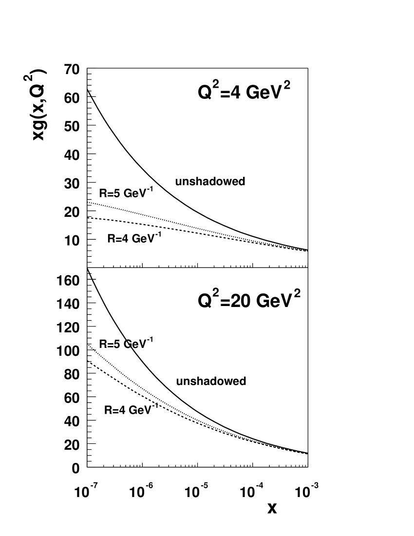
Figure 1: The effect of shadowing on the integrated gluon distribution $xg(x,Q^{2})$, at $Q^{2}=4~{}{\rm GeV}^{2}$ and $20~{}{\rm GeV}^{2}$. The continuous line is simply the unshadowed $xg$ obtained from $f_{L}$ [22]. The dashed and dotted lines show the result of shadowing with $R=4$ and $5\ {\rm GeV}^{-1}$ respectively, where the ‘radius’ $R$ is defined in (16) in terms of the proton profile function, $S(b)$.

References

- [1] L.V. Gribov, E.M. Levin and M.G. Ryskin, Phys. Rep. 100 (1983) 1.
- [2] A.H. Mueller and J. Qiu, Nucl. Phys. B268 (1986) 427.
- [3] N.N. Nikolaev and B.G. Zakharov, Z. Phys. C49 (1991) 607; Z. Phys C53 (1992) 331; Z. Phys. C64 (1994) 651; JETP 78 (1994) 598.
- [4] A. H. Mueller, Nucl. Phys. B415 (1994) 373; A. H. Mueller and B. Patel, Nucl. Phys. B425 (1994) 471; A. H. Mueller, Nucl. Phys. B437 (1995) 107.
- [5] A.H. Mueller, Nucl. Phys. B335 (1990) 115; Yu.A. Kovchegov, A.H. Mueller and S. Wallon, Nucl. Phys. B507 (1997) 367. A.H. Mueller, Eur. Phys. J. A1 (1998) 19; Nucl.Phys. A654 (1999) 370; Nucl.Phys. B558 (1999) 285.
- [6] J. C. Collins and J. Kwieciński, Nucl. Phys. B335 (1990) 89.
- [7] J. Bartels, G.A. Schuler and J. Blümlein, Z. Phys. C50 (1991) 91; Nucl. Phys. Proc. Suppl. 18 C (1991) 147; J. Bartels, Phys. Lett. B298 (1993) 204; Z. Phys. C60 (1993) 471; Z. Phys. C62 (1994) 425; J. Bartels and M. Wüsthoff, Z. Phys. C66 (1995) 157; J. Bartels and C. Ewerz, JHEP 9909 (1999) 026.
- [8] J. Bartels and E. M. Levin, Nucl. Phys. B387 (1992) 617.
- [9] L. McLerran and R. Venugopalan, Phys. Rev. D49 (1994) 2233, Phys. Rev. D49 (1994) 3352, Phys. Rev. D50 (1994) 2225; A. Kovner, L. McLerran and H. Weigert, Phys.Rev. D52 (1995) 6231, Phys. Rev. D52 (1995) 3809; R. Venugopalan, Acta. Phys. Polon. B30 (1999) 3731.
- [10] A. Białas and R. Peschanski, Phys. Lett. B355 (1995) 301; Phys. Lett. B378 (1996) 302; Phys. Lett. B387 (1996) 405; A. Bialas Acta Phys. Polon. B28 (1997) 1239; A. Bialas and W. Czyz, Acta Phys.Polon. B29 (1998) 2095; A. Białas, H. Navelet and R. Peschanski, Phys. Rev. D57 (1998) 6585; Phys. Lett. B427 (1998) 147.
- [11] A.Białas, H.Navelet and R. Peschanski, Nucl. Phys. B593 (2001) 438.
- [12] G.P. Salam, Nucl. Phys. B449 (1995) 589; Nucl. Phys. B461 (1996) 512; Comput. Phys. Commun. 105 (1997) 62; A.H. Mueller and G.P. Salam, Nucl. Phys. B475 (1996) 293.
- [13] E. Gotsman, E. M. Levin and U. Maor, Nucl. Phys. B464 (1996) 251; Nucl. Phys. B493 (1997) 354; Phys. Lett. B245 (1998) 369; Eur. Phys. J. C5 (1998) 303; E. Gotsman, E. M. Levin, U. Maor and E. Naftali, Nucl. Phys. B539 (1999) 535; A. L. Ayala Filho, M. B. Gay Ducati and E. M. Levin, Nucl.Phys. B493 (1997) 305; Nucl. Phys. B551 (1998) 355; Eur. Phys. J. C8 (1999) 115; E. Levin and U. Maor, hep-ph/0009217.
- [14] Ia. Balitsky, Nucl. Phys. B463 (1996) 99.
- [15] J. Jalilian-Marian, A. Kovner, L. McLerran and H. Weigert, Phys. Rev. D55 (1997) 5414; J. Jalilian-Marian, A. Kovner and H. Weigert, Phys. Rev. D59 (1999) 014014; Phys. Rev. D59 (1999) 014015; Phys. Rev. D59 (1999) 034007; Erratum-ibid. D59 (1999) 099903; A. Kovner, J.Guilherme Milhano and H. Weigert, Phys. Rev. D62 (2000) 114005; H. Weigert, NORDITA-2000-34-HE, hep-ph/0004044.
- [16] M.A. Braun, Eur. Phys. J. C16 (2000) 337; hep-ph/0101070 .
- [17] Y.V. Kovchegov, Phys. Rev. D60 (1999) 034008; Phys. Rev. D61 (2000) 074018.
- [18] E.A. Kuraev, L.N. Lipatov and V.S. Fadin, Sov. Phys. JETP 44 (1976) 443; ibid. 45 (1977) 199; I.I. Balitsky and L.N. Lipatov, Sov. J. Nucl. Phys. 28 (1978) 822.
- [19] E. M. Levin and K. Tuchin, Nucl. Phys. B537 (2000) 833; hep-ph/0012167.
- [20] Y.V. Kovchegov and L. McLerran, Phys. Rev. D60 (1999) 054025; Erratum-ibid. D62 (2000) 019901; Y.V. Kovchegov and E. M. Levin, Nucl. Phys. B577 (2000) 221.
- [21] Zhang Chen and A.H. Mueller, Nucl. Phys. B451 (1995) 575.
- [22] J. Kwiecinski, A.D. Martin and A.M. Stasto, Phys. Rev. D56 (1997) 5867.
- [23] A. De Roeck, Contribution to the First Workshop on Forward Physics at the LHC, Helsinki, Nov. 2000.