Neutrinos from Stellar Collapse:
Comparison of signatures in water and heavy water detectors

Abstract

Signatures of neutrino and antineutrino signals from stellar collapse in heavy water detectors are contrasted with those in water detectors. The effects of mixing, especially due to the highly dense matter in the supernova core, are studied. The mixing parameters used are those sets allowed by current understanding of available neutrino data: from solar, atmospheric and laboratory neutrino experiments. Signals at a heavy water detector, especially the dominant charged current reactions on deuteron, are very sensitive to some of these sets of allowed mixing parameters. Theoretical uncertainties on supernova neutrino spectra notwithstanding, a combination of supernova measurements with water and heavy water detectors may be able to distinguish many of these mixing possibilities and thus help in ruling out many of them.

I Introduction

Neutrinos from stellar collapse have so far been detected only from the supernova SN1987a in the Large Magellanic Cloud[1]. The inital observations of the neutrino and antineutrino events by the Kamiokande[2] and IMB[3] collaborations were the subject of detailed analysis by several authors [4, 5, 6, 7, 8, 9, 10] immediately following the event. The analyses confirmed the qualitative features of core collapse and subsequent neutrino emission.

The effect of non-zero neutrino masses and mixing on supernova signals was first analysed in general by Kuo and Pantaleone[11]. Recently, several authors have looked at the possible signatures of neutrinos and antineutrinos from supernova collapse in realistic scenarios. Dighe and Smirnov[12] have looked at the problem of reconstruction of the neutrino mass spectrum in a three-flavour scenario. These authors as also Chiu and Kuo[13] have compared the signatures in the standard mass hierarchy and inverted mass hierarchy. While these papers incorporate the constraints from solar and atmospheric neutrino observations, the important question of the mass limits that may be obtained from the observation of time delay has been analysed by Beacom and Vogel[14, 15] and by Choubey and Kar[16] (see also the review by Vogel[17]). For a recent review which also discusses aspects of locating a supernova by its neutrinos in advance of optical observation, see Ref. [18].

In this paper we apply the analysis of neutrinos from stellar collapse presented in Refs. [19, 20] to heavy water detectors. We had previously discussed in detail the signatures, in a water Cerenkov detector, of neutrinos and antineutrinos from stellar collapse in both 3- and 4-flavour mixing scenarios. The 4-flavour analysis was motivated by lsnd data [21]. The analysis was confined to Type II supernovae (which occur when the initial mass of the star is larger than 8 solar masses). The choices of mixing parameters used were consistent with available data on solar, atmospheric and laboratory neutrino experiments. It turns out that different choices of (allowed) mixing parameters lead to drastically different supernova signals at water detectors. While certain features are common to both the 3- and 4-flavour analyses, there are important differences that may (depending on the mixing parameters) be able to distinguish the number of flavours. We will summarise the salient features of this analysis below.

The dominant contribution is from the charged current (CC) scattering of $\overline{\nu}_{e}$ on protons in water. Mixing can increase the number of high energy events in this channel. The most dramatic effect of 3-flavour mixing is to produce a sharp increase in the CC events involving oxygen targets [19, 22] for most choices of mixing parameters. These will show up as a marked increase in the number of events in the backward direction with respect to the forward peaked events involving electrons as targets (more than 90% of which lie in a $10^{\circ}$ forward cone with respect to the supernova direction for neutrinos with energies $E_{\nu}~{}{\stackrel{{\scriptstyle{}_{\displaystyle>}}}{{{}_{\displaystyle\sim}}}}~{}8$ MeV), both showing up over the mostly isotropic CC events on protons. In the absence of such mixing, there will be only a few events due to CC scattering on oxygen targets. These events involving oxygen targets will be seen in a heavy water detector as well; realistically however, there will be fewer such events due to the considerably smaller size of the heavy water detector at the Sudbury Neutrino Observatory (sno) as compared to the water detector at SuperKamiokande (SuperK).

When 4-flavour mixing is considered, the analysis becomes obviously more complex; now, the increase due to oxygen events will be visible only for some of the allowed values of the parameters. Furthermore, there is no set of allowed parameters in both the 3- and 4-flavour cases for which the signals in a water detector will be able to distinguish between adiabatic and non-adiabatic neutrino propagation in the core of the supernova. This is an important issue since it can place a lower bound on the (13) mixing angle, which is currently bounded by chooz at the upper end in the case of 3-flavour mixing. (The only non-zero value for this angle so far comes from the lsnd data which can only be analysed in a 4-flavour frame-work). A zero value for this mixing angle will decouple the two sets of oscillations, $\nu_{e}\to\nu_{\mu}$ and $\nu_{\mu}\to\nu_{\tau}$, and allow for a simple 2-flavour analysis separately of the solar and atmospheric neutrino data. An exactly zero value of this angle will also render irrelevant CP violating phases in the problem.

There are also CC and neutral current (NC) events due to elastic scattering with electrons in water/heavy water. These interactions are the same in both detectors and have been discussed in detail in the earlier analysis on water detectors [20].

In this paper we focus on the possible signatures of a supernova collapse in a heavy water detector. The question is of practical interest since sno is operating for more than a year now. It turns out that a combination of measurements in water and heavy water detectors has much better discriminatory power than either of them individually. Hence such observations of supernova neutrinos may be a good signal to rule out some of the currently allowed parameter space in the neutrino mixing angles. (These signals are however not very sensitive to neutrino mass squared differences.)

The most interesting signals to study at a heavy water detector are the events from CC interactions of both $\nu_{e}$ and $\overline{\nu}_{e}$ on deuterons. This is the most dominant signal in contrast to the dominant CC interaction of $\overline{\nu}_{e}$ alone on free protons in a water detector (all are typically about two orders of magnitude larger than those from oxygen or electron interactions). We will focus mostly on these events in this paper, besides making a few remarks on the NC events on deuteron that can also easily be measured at a heavy water detector. These are therefore the “new” signals in a heavy water detector that would not be observable in (or will be different from) a water detector.

As before the analysis is done assuming the standard mass hierarchy necessitated by the solar and atmospheric neutrino observations [23]. We also impose all the known constraints on the mixing parameters and mass-squared differences including those constraints from laboratory experiments[21, 24]. The purpose of the calculation is to see whether different mixing scenarios give significantly different signals in the detector.

In Sect. II we briefly outline the frame-work including the mixing matrix as also matter effects on mixing. We then use this to obtain expressions for the $\nu_{e}$, $\overline{\nu}_{e}$ and $\nu_{\mu,\tau}$, $\overline{\nu}_{\mu,\tau}$ fluxes reaching the detector in both 3- and 4-flavour mixing schemes. While discussions may be found in Ref. [19, 20] we reproduce the relevant details to keep this paper self-contained. In Sect. III we list the different interaction processes relevant to both water and heavy water detectors, in particular, those with electrons (positrons) in the final state, as well as NC events on deuteron. The details of the supernova model used in the calculation as well as the allowed values of neutrino mixing parameters (from already existing data) using which the effects of mixing are computed are also listed here. Results showing the effects of mixing both for the spectrum and the integrated number of events are presented in Sect. IV. Sensitivity to the supernova model parameters is discussed. The NC events on deuterons in a heavy water detector are also briefly discussed here. All these results are for a $(2+2)$ mass hierarchy scheme in the case of 4 flavour mixing. In Sect. V, we briefly discuss the other possible scenario, that of the $(3+1)$ scheme in 4-flavours. We present a summary and discussions in Sect. VI.

II Neutrino mixing and matter effects

We briefly review mixing among three and four flavours of neutrinos (or antineutrinos) and compute the neutrino (antineutrino) survival and conversion probabilities. These are given in more detail in Refs.[19, 20]. The supernova neutrinos are produced mostly in the core, where the matter density is very high. Hence matter effects on the propagation are important.

The hierarchy of mass eigenstates is shown in Fig. 1. The 3-flavour case is shown in Fig. 1a; there are essentially two scales corresponding to the solution of solar and atmospheric neutrino problems assuming neutrino oscillations. In the case of four flavours (necessitated by the non-zero result of lsnd [21]), the analysis is more complicated since there is an additional sterile neutrino. One possible mass hierarchy here is a $(2+2)$ scenario [25] as shown in Fig. 1b. The lsnd result implies the existence of a mass scale in the range of 0.1 eV² to 1 eV². We choose two doublets separated by this mass scale. The intra-doublet separation in the lower doublet corresponds to the solar neutrino scale $~{}{\stackrel{{\scriptstyle{}_{\displaystyle<}}}{{{}_{\displaystyle\sim}}}}~{}10^{-5}$ eV² and that in the upper one to the atmospheric neutrino scale $\sim 10^{-3}$ eV². Yet another possibility is the so-called $(3+1)$ scheme [26, 27], where the 3-flavour scheme is extended by adding a heavy sterile neutrino as the heaviest mass eigenstate, with a mass separation from the other three states as required by lsnd. We discuss this scheme separately later. In what follows, therefore, 4-flavour mixing always refers to the $(2+2)$ scheme.

The mixing matrix, $U$, which relates the flavour and mass eigenstates in the above scenarios has three angles in the 3-flavour case and six angles in the 4-flavour one. We shall ignore the CP violating phases. Then, the mixing matrix can be parametrised in the case of 3-flavours as,

$$\left[\nu_{e}\quad\nu_{\mu}\quad\nu_{\tau}\right]^{T}=U\times\left[\nu_{1}\quad\nu_{2}\quad\nu_{3}\right]^{T}~{},$$ (1)

where $T$ stands for transpose. Here $U$ is parametrised by considering rotations of mass eigenstates taken two at a time:

$$U = U_{23}\times U_{13}\times U_{12}~{},$$ (2)

$$= U_{\psi}\times U_{\phi}\times U_{\omega}~{},$$ (3)

where $U_{ij}$ corresponds to the rotation of mass eigenstates $|i\rangle$ and $|j\rangle$. As is the convention, we denote the mixing angle relevant to the solar neutrino problem by $\omega$ and that relevant to the atmospheric neutrino problem by $\psi$ in the case of 3 flavours. The (13) angle $\phi$ is then small, due to the chooz result [24] which translates to the constraint on the (13) mixing angle, $\sin\phi\equiv\epsilon\leq\epsilon_{0}$, where $\epsilon_{0}=0.16$. In the case of 4-flavours, we choose to work in the $(2+2)$ scheme:

$$\left[\nu_{e}\quad\nu_{s}\quad\nu_{\mu}\quad\nu_{\tau}\right]^{T}=U\times\left[\nu_{1}\quad\nu_{2}\quad\nu_{3}\quad\nu_{4}\right]^{T}~{},$$ (4)

where the mixing matrix is similarly defined to be,

$$U = U_{34}\times U_{24}\times U_{23}\times U_{14}\times U_{13}\times U_{12}~{},$$ (5)

$$= U_{\psi}\times U_{\epsilon}\times U_{\epsilon}\times U_{\epsilon}\times U_{\epsilon}\times U_{\omega}~{}.$$ (6)

Here the (13) and (14) angles are constrained by chooz to be small: $\theta_{13},\theta_{14}\sim\epsilon\leq\epsilon_{0}$ [20]. The atmospheric neutrino problem constrains $\theta_{34}$ (the equivalent of the angle $\psi$ in the 3-flavour case) to be maximal, when both $\theta_{23},\theta_{24}$ become small. We shall assume they are also limited by the same small parameter, $\epsilon_{0}$.

The other relevant definition is the chosen mass hierarchy in the problem. We define the mass squared differences as $\delta_{ij}=\mu_{i}^{2}-\mu_{j}^{2}$, where $i,j$ run over the number of flavours. Without loss of generality, we can take $\delta_{21}$, $\delta_{31}$ (and $\delta_{41}$) to be greater than zero; this defines the standard hierarchy of masses consistent with the range of the mixing angles, as specified above.

A Matter effects for neutrinos

The most important consequence of the highly dense core matter is to cause Mikheyev, Smirnov and Wolfenstein (MSW) resonances [29] in the neutrino sector. (The chosen mass hierarchy prevents such resonances from occurring in the antineutrino sector). In both the 3- and 4-flavour cases, this causes the electron neutrino to occur essentially as a pure mass state [20], in fact, as the highest mass eigenstate, as can be seen from the schematic illustration in Fig. 2. Nonadiabatic transitions near the resonances will alter this result, especially in the case of 4-flavours, where there are several level crossings because of the presence of the sterile neutrino. Hence we will discuss the purely adiabatic and the non-adiabatic cases separately.

1 The adiabatic case

We begin with the 3-flavour case. The average transition probability from flavour $\beta$ to flavour $\alpha$ is denoted by $P_{\alpha\beta}$ where $\alpha,\beta$ run over all flavours. It turns out that, independent of other mixing angles and the mass squared differences, the survival probability for the adiabatic case is,

$$P_{ee}=\epsilon^{2}~{},$$ (7)

and hence is small. This is sufficient to determine all the relevant fluxes in the 3-flavour case. In the 4-flavour adiabatic case, we again have,

$$P_{ee}=\epsilon^{2}~{},$$ (8)

so that the electron neutrino survival probability is flavour independent in the adiabatic case. In addition, we also need to know some other probabilities in order to compute the fluxes at the detector. We have

$$P_{es}=P_{se}=P_{ss}=P_{ee}=\epsilon^{2}~{}.$$ (9)

2 The non-adiabatic case

Because of the parametrisation it is easy to see that non-adiabatic effects in the form of Landau Zener (LZ) jumps are introduced as a result of the values chosen for $\epsilon$ and $\omega$. The value of $\epsilon$ determines whether non-adiabatic jumps are induced at the upper resonance(s) while the value of $\omega$ determines whether the non-adiabatic jump occurs at the lower resonance. This statement holds both for three and four flavours since in both cases the non-adiabaticity in the upper resonance(s) is controlled by $\epsilon$, apart from mass squared differences.

For a large range of $\epsilon$, allowed by the chooz constraint, the evolution of the electron neutrino is adiabatic. As a result the lower resonance does not come into the picture at all except when $\epsilon$ is very close to zero, where the LZ jump probability at the upper resonance(s), $P_{H}$, abruptly changes to one [11, 30]. This occurs in a very narrow window: for instance, when $\epsilon$ changes from 0.02 to 0.01 $P_{H}$ changes from 0.01 to 0.34 for a mass scale in the range of $10^{-3}$ eV². The subsequent discussion is therefore relevant only when $\epsilon$ is vanishingly small, $\epsilon\ll 10^{-2}$. (This is not ruled out by the known constraints except lsnd).

The LZ transition at the lower resonance is determined by the probability, $P_{L}$, which is a function of the mixing angle $\omega$ and the mass squared difference $\delta_{21}$. It turns out that $P_{L}$ is zero unless $\omega$ is small, $\sin\omega~{}{\stackrel{{\scriptstyle{}_{\displaystyle<}}}{{{}_{\displaystyle\sim}}}}~{}0.2$ for mass differences in the solar neutrino range $\sim 10^{-5}$ eV². This case (of small $\epsilon$, small $\omega$) corresponds to the extreme non-adiabatic limit. When $\omega$ is large, as in the case of the large-angle MSW or the vacuum solution to the solar neutrino problem, non-adiabaticity occurs only at the upper resonance and is therefore partial.

In our calculations we have used the form for $P_{H}$ and $P_{L}$ discussed in the appendix of Ref.[19] (see also [30]). Because of the sharpness of the transition at the upper resonance we will set $P_{H}=1$ for small enough $\epsilon$ and only consider the dependence of the survival probability on the LZ transition at the lower resonance.

In the 3-flavour non-adiabatic case the only relevant probability is,

$$P_{ee}=(1-\epsilon^{2})[(1-P_{L})\sin^{2}\omega~{}+P_{L}\cos^{2}\omega]~{}.$$ (10)

In the non-adiabatic 4-flavour case we have,

$$P_{ee} = (1-2\epsilon^{2})[(1-P_{L})\sin^{2}\omega~{}+P_{L}\cos^{2}\omega]~{},$$ (11)

$$P_{es} = (1-2\epsilon^{2})[(1-P_{L})\cos^{2}\omega~{}+P_{L}\sin^{2}\omega]~{}.$$ (12)

Since $\epsilon$ is small, the flux at the detector is entirely controlled by $\omega$ and $P_{L}$ which is also a function of $\omega$. Note that the sum $P_{ee}+P_{es}=1-2\epsilon^{2}$ is independent of $P_{L}$ in 4-flavours. Since $P_{ee}+P_{es}=1-P_{e\mu}-P_{e\tau}$, this also indicates that the probability of transition of $\nu_{\mu,\tau}$ into $\nu_{e}$ is small in the non-adiabatic case, in contrast to the adiabatic case where $P_{ee}+P_{es}=2\epsilon^{2}$.

B Matter effects for antineutrinos

Due to our choice of mass hierarchy, the propagation of antineutrinos is always adiabatic (the matter dependent term has the opposite sign as compared to neutrinos). Here also the high density of matter in the core causes the electron antineutrino to be produced as a pure mass eigenstate, $\overline{\nu}_{1}$.

In the 3-flavour case, we have

$$P_{\overline{e}\overline{e}}=(1-\epsilon^{2})\cos^{2}\omega~{}.\\$$ (13)

In the 4-flavour case, we have,

$$P_{\overline{e}\overline{e}} = (1-2\epsilon^{2})\cos^{2}\omega~{},$$ (14)

$$P_{\overline{e}\overline{s}} = (1-2\epsilon^{2})\sin^{2}\omega~{}.$$ (15)

Hence, when $\omega$ is small, there is very little loss of the $\overline{\nu}_{e}$ flux into the sterile channel. Also, the sum $P_{\overline{e}\overline{e}}+P_{\overline{e}\overline{s}}=(1-2\epsilon^{2})$ is similar to the non-adiabatic neutrino propagation so that very little $\overline{\nu}_{\mu,\tau}$ is converted to $\overline{\nu}_{e}$.

For the NC events, we will also need the following:

$$P_{\overline{s}\overline{e}} = (1-2\epsilon^{2})\sin^{2}\omega+2\epsilon^{2}\sin 2\omega~{},$$ (16)

$$P_{\overline{s}\overline{s}} = (1-2\epsilon^{2})\cos^{2}\omega-2\epsilon^{2}\sin 2\omega~{}.$$ (17)

These probabilities can then be used to determine the observed antineutrino fluxes.

C The neutrino (antineutrino) fluxes at the detector

Following Kuo and Pantaleone [11], we denote the flux distribution, ${\rm d}\phi_{\alpha}^{0}/{\rm d}E$, of a neutrino (or antineutrino) of flavour $\alpha$ with energy $E$ produced in the core of the supernova by $F_{\alpha}^{0}$. In particular we use the generic label $F_{x}^{0}$ for flavours other than $\nu_{e}$ and $\overline{\nu}_{e}$ since

$$F_{x}^{0}=F_{\overline{x}}^{0}=F_{{\mu}}^{0}=F_{\overline{\mu}}^{0}=F_{{\tau}}^{0}=F_{\overline{\tau}}^{0}~{}.$$ (18)

Typically, models for supernovae predict that the $\overline{\nu}_{e}$ and $\nu_{x}$ have hotter spectra than $\nu_{e}$. This is because the $\nu_{x}$ decouples first since it has only NC interactions with matter and therefore leaves the cooling supernova with the hottest thermal spectrum. The CC interactions of $\nu_{e}$ with matter are larger than those of $\overline{\nu}_{e}$ and hence $\nu_{e}$ has the coldest spectrum. The model on which this work is based [31] predicts that the average energies of the $\nu_{e}$, $\overline{\nu}_{e}$ and $\nu_{x}$ spectra are around 11, 16, and 25 MeV. We make our observations, keeping this in mind.

The $\nu_{e}$ flux on earth is given in terms of the flux of neutrinos produced in the core of the supernova by,

$$F_{e} = P_{ee}F_{e}^{0}+P_{e\mu}F_{{\mu}}^{0}+P_{e\tau}F_{{\tau}}^{0},$$ (19)

$$= P_{ee}F_{e}^{0}+(1-P_{ee})F_{x}^{0}\qquad\qquad(\hbox{\rm 3-flavours)}~{},$$ (20)

$$= P_{ee}F_{e}^{0}+(1-P_{ee}-P_{es})F_{x}^{0}~{}\quad(\hbox{\rm 4-flavours)}~{},$$ (21)

where we have made use of the constraint $\sum_{\beta}P_{\alpha\beta}=1$. This flux is further reduced by an overall geometric factor of $1/(4\pi d^{2})$ for the case of a supernova at a distance $d$ from the earth.

Since the probabilities $P_{ee}$ and $P_{es}$ are known, the $\nu_{e}$ flux can be computed in terms of the original fluxes emitted by the supernova.

The $\nu_{e}$ flux is independent of the (12) mixing angles $\omega$ in the adiabatic case. Also, it is not very different for 3- and 4-flavours. In both, the observed flux is almost entirely due to the original $\nu_{x}$ flux since $P_{ee}=\epsilon^{2}$ is small, and is therefore hotter.

From Eq. (12) we see that, in contrast, the contribution from the hotter spectrum into electron neutrinos in the 4-flavour non-adiabatic case is controlled entirely by $\epsilon$ and is small. However, the observed flux can be depleted, depending on the value of $P_{L}$. The signal in the 3-flavour case is drastically different because the contribution of the hotter spectrum now depends on $\epsilon$, $\omega$ and $P_{L}$. In general, the possibility of LZ transitions makes the analysis more complicated. We will discuss this case numerically later.

The result for $\overline{\nu}_{e}$ is the same, with $P_{ee}$ replaced by $P_{\overline{e}\overline{e}}$, etc. For example,

$$F_{\overline{e}} = P_{\overline{e}\overline{e}}F_{\overline{e}}^{0}+(1-P_{\overline{e}\overline{e}})F_{x}^{0}\qquad\qquad(\hbox{\rm 3-flavours)}~{},$$ (22)

$$= P_{\overline{e}\overline{e}}F_{\overline{e}}^{0}+(1-P_{\overline{e}\overline{e}}-P_{\overline{e}\overline{s}})F_{x}^{0}~{}\quad(\hbox{\rm 4-flavours)}~{}.$$ (23)

There is hardly any mixing of the hotter spectrum into electron antineutrinos in the 4-flavour case since $(1-P_{\overline{e}\overline{e}}-P_{\overline{e}\overline{s}})=2\epsilon^{2}$ is small. The extent of mixing in 3-flavours depends on the value of $\omega$ through $P_{\overline{e}\overline{e}}$. For small $\omega$, there is very little change in the electron antineutrino flux (see Eq. (15)).

The results are summarised in Tables I and  II for the adiabatic neutrino and antineutrino cases, and in Table III for non-adiabatic neutrino propagation. Expressions for the other flavours, needed to compute the NC events, are also given in these tables. For instance,

$$2F_{x} = F_{{\mu}}+F_{{\tau}}~{},$$ (24)

$$= (P_{ee}+P_{es}+P_{se}+P_{ss})F_{x}^{0}+(1-P_{ee}-P_{se})F_{e}^{0}~{}\qquad\hbox{(4 flavours)}~{}.$$ (25)

A similar expression holds for $F_{\overline{x}}$ with $P_{\alpha\beta}$ replaced by $P_{\overline{\alpha}\overline{\beta}}$.

While the neutral current (NC) combination, $(\nu_{e}+2\nu_{x}+\overline{\nu}_{e}+2\overline{\nu}_{x})$, remains unaltered in 3-flavours, there may be actual loss of spectrum into the sterile channel in the 4-flavour case. This should also be a good indicator of the number of flavours involved in the mixing.

Water as well as heavy water detectors will be sensitive to all these aspects of mixing. In the next section, we will discuss the inputs and constraints, both from supernova models as well as current neutrino experiments. These will then be used subsequently to predict numerically supernova event rates.

III Inputs and Constraints

We will concentrate mostly on the dominant CC and NC interactions of $\nu_{e}$ and $\overline{\nu}_{e}$ on deuteron in heavy water. We will also compare the CC interactions to those at a water detector, that is, to $\overline{\nu}_{e}$ on protons. Interactions on electrons and oxygen nuclei in water and heavy water detectors are the same, and have been discussed in detail in Refs. [19, 20].

A Interaction processes and relevant formulae

Both in water and heavy water detectors, the interactions we are mainly interested in are of three types:

1. Dominant events: These are due to the CC $\overline{\nu}_{e}\,p\to e^{+}\,n$ interaction in water. In heavy water, there are contributions from both $\overline{\nu}_{e}\,d\to e^{+}\,nn$ and ${\nu}_{e}\,d\to e^{-}\,pp$ CC processes. At the neutrino energies relevant to this discussion, the cross-sections for these processes, and hence the number of events, are about two orders of magnitude larger than any of the others.

2. Electron events: These are due to elastic scatterings of $\nu_{e}$, $\overline{\nu}_{e}$, $\nu_{x}$, $\overline{\nu}_{x}$ on electron targets in both water and heavy water.

3. Oxygen events: These arise from CC scattering of $\nu_{e}$ and $\overline{\nu}_{e}$ on oxygen nuclei in both detectors.

In all these cases, the events are identified by detecting an electron (or positron) in the final state. The electron events, although small in number, are highly forward peaked [32]. The oxygen events have a high energy threshold ($E_{\nu_{e}}>15.4$ MeV; $E_{\overline{\nu}_{e}}>11.4$ MeV) and can only occur if there is substantial mixing of the hotter $\nu_{x}$ spectrum with the $\nu_{e}$ or the $\overline{\nu}_{e}$ in which case these events are highly backward peaked [22]. Both these may therefore be readily separated from the mostly isotropic dominant events in water [34]. In the case of heavy water, the angular distribution of both the dominant processes is well-known [34, 35, 36] and is approximately given by

$$P(\theta)\propto 1-{\displaystyle{1}\over\displaystyle{3}}\cos\theta~{},$$

at the energies of interest. Here $\theta$ is the electron (positron) laboratory scattering angle. So there are typically twice as many events in the backward direction as in the forward direction. This makes the exclusive identification of oxygen events more difficult in a heavy water detector.

A note on the nomenclature “forward” and “backward”. We envisage the angular dependence as being measured in typically six bins of $30^{\circ}$ each, the first bin corresponding to “forward” and the last one corresponding to the “backward” events. This obviates the need for very accurate angle measurements as well as takes into consideration effects like electron-rescattering that may smear out the scattering angle. This bin size is also typically what is available at SuperKamiokande.

Since the supernova signal is a short and well-defined signal (lasting about 10 secs), it will be possible to detect all these events over background (due to solar and other radioactive processes). For instance, in the relevant energy region, SuperKamiokande reports [37] a background of 0.2 events/day/kton in a bin of 1 MeV of scattered electron energy from the direction of the sun, and half that rate from all other scattering angles. The corresponding number for SNO is not available, although the radioactive background is expected to be small compared to the solar signal [38]. Furthermore, since their angular distribution is well-known, angular information on the final state electron ($e^{-}$ or $e^{+}$) may allow us to separate out these three types of events. The detailed analysis of signals due to mixing in the forward and backward event samples is given in Ref.[20] for a water Cerenkov detector. These results also hold for a heavy water detector (apart from a scaling factor of 0.9 due to the mass difference between water and heavy water). We will not discuss this further and concentrate on the new results for the CC events on deuterons. In addition, there are NC processes on the deuteron in heavy water that may be detected by the subsequent neutron capture and the associated gamma rays.

The specific processes we will consider, for water and heavy water detectors, therefore are

$$\overline{\nu}_{e}+p\to e^{+}+n~{},$$ (26)

and

$$\overline{\nu}_{e}+d \to e^{+}+n+n~{},$$ (27)

$$\nu_{e}+d \to e^{-}+p+p~{}.$$ (28)

Common to both detectors are the processes,

$$\nu_{\alpha}+e \to \nu_{\alpha}+e\qquad(\alpha=e,x,\overline{e},\overline{x})~{},$$ (29)

$$\nu_{e}+{}_{8}^{16}O \to e^{-}+X~{},$$ (30)

$$\overline{\nu}_{e}+{}_{8}^{16}O \to e^{+}+X~{},$$ (31)

where the elastic scattering on electrons involves both CC and NC interactions.

We will also discuss the interesting possibility of observing NC events on deuteron in a heavy water detector:

$$\overline{\nu}+d \to \overline{\nu}+n+p~{},$$ (32)

$$\nu+d \to \nu+n+p~{}.$$ (33)

The cross-sections for Eqs. (26)–(33) are well-known [32, 33, 22]. The $\overline{\nu}_{e}p$ cross-section is large in water Cerenkov detectors, being proportional to the square of the antineutrino energy. In terms of total number of events, therefore, water Cerenkov detectors are mostly dominated by $\overline{\nu}_{e}\,p$ events. The deuteron CC cross sections are comparable though the $\nu_{e}$ CC reaction on deuteron has a slightly lower threshold and a somewhat larger cross-section than the $\overline{\nu}_{e}$ CC. Also, the $\overline{\nu}_{e}$ CC cross-section in heavy water is about 4 times smaller than the corresponding one in water due to Pauli suppression.

When the recoil electron (positron) is detected, the time integrated event rate due to neutrinos (or antineutrinos) of flavour $\alpha$ and energy $E$ on target $T$, as a function of the recoil electron (or positron) energy, $E_{e}$, is as usual given by,

$${\displaystyle{{\rm d}N_{\alpha}^{\rm T}(E_{e})}\over\displaystyle{{\rm d}E_{e}}}={\displaystyle{n_{T}}\over\displaystyle{4\pi d^{2}}}\sum_{b}\Delta t_{b}\int{\rm d}EF_{\alpha}(b){\displaystyle{{\rm d}\sigma^{\rm T}}\over\displaystyle{{\rm d}E_{e}}}~{}.$$ (34)

The index $b$ refers to the time interval within which the (original) thermal neutrino spectrum can be assumed to be at a constant temperature $T_{b}(\alpha)$. Here $n_{T}$ refers to the number of scattering targets (of $d$, $p$, $e$, or $O$) that are available in the detector. Also, for processes involving $d$ and $p$, the hadron recoil is so small that we assume $E_{e}=E-\delta_{IF}$, where $\delta_{IF}$ is the mass difference between the initial and final hadrons (including the binding energy). While this results in a small threshold of a few MeV in these cases, the threshold for oxygen processes is greater than 10 MeV. The total number of events from a given flavour of neutrino in a given bin, $k$, of electron energy (which we choose to be of width 1 MeV) then is

$$N_{\alpha}^{T}(k)=\int_{k}^{k+1}{\rm d}E_{e}{\displaystyle{{\rm d}N_{\alpha}^{\rm T}}\over\displaystyle{{\rm d}E_{e}}}~{}.$$ (35)

In the case of NC events in heavy water, the total number of events is calculated according to

$$N_{\alpha}^{\rm NC}={\displaystyle{n_{t}}\over\displaystyle{4\pi d^{2}}}\sum_{b}\Delta t_{b}\int{\rm d}EF_{\alpha}(b)\sigma^{\rm NC}(E)~{}.$$ (36)

Here again the cross-section is well-known [33].

B The supernova flux inputs

As in [19, 20], we compute the time integrated event rate at prototype 1 kton water and heavy water detectors from neutrinos emitted by a supernova exploding 10 kpc away. Results for any other supernova explosion may be obtained by scaling the event rate by the appropriate distance to the supernova and the size of the detector, as shown in Eq. (34). We assume the efficiency and resolution of the detectors to be perfect; this will only slightly enhance the event rates near the detector threshold [20].

We use the luminosity and average energy distributions (as functions of time) for neutrinos of flavour $\alpha$ and energy $E$ as given in Totani et al. [31], based on the numerical modelling of Mayle, Wilson and Schramm [39]. In a short time interval, $\Delta t_{b}$, the temperature can be set to a constant, $T_{b}(\alpha)$. Then the neutrino number flux can be described, in this time interval, by a thermal Fermi Dirac distribution,

$$F_{\alpha}^{0}(b)=N_{0}{\displaystyle{{\cal L}_{b}(\alpha)}\over\displaystyle{T_{b}^{4}(\alpha)}}{\displaystyle{E^{2}}\over\displaystyle{(\exp(E/T_{b}(\alpha))+1)}}~{},$$ (37)

at a time $t$ after the core bounce. Here $b$ refers to the time-bin, $t=t_{0}+b\Delta t$. We set the time of bounce, $t_{0}=0$. The overall normalisation, $N_{0}$, is fixed by requiring that the total energy emitted per unit time equals the luminosity, ${\cal L}_{b}(\alpha)$, in that time interval. The precise values for ${\cal L}_{b}(\alpha)$ and $T_{b}(\alpha)$ are taken from Ref. [31]. The total emitted energy in all flavours of neutrinos is about $2.7\times 10^{53}$ ergs. The general features of the model are as follows: The temperature is roughly constant over the entire period of emission (lasting roughly 10 seconds). Typical values are $T_{b}(\alpha)=3.15\langle E\rangle_{\alpha}$, with the average energy of each flavour, $\langle E\rangle_{\alpha}=11,16,25$ MeV for $\alpha=\nu_{e},\overline{\nu}_{e}$ and $\nu_{x}$ respectively. Also, the total emitted energy is more or less equally distributed in all flavours. (The luminosity of $\nu_{e}$ is higher than that of other flavours at early times, while that of $\nu_{x}$ is higher after 1 sec). The number of neutrinos emitted in each flavour, however, is not the same since their average energies are different. While we use the values for the time dependent temperature and luminosity as given by Ref. [31] in our analysis, we also examine the effects due to possible variations of these parameters and hence the sensitivity of our results to the details of the supernova model used.

With large matter effects present in both the neutrino and antineutrino sector, the validity of the average energies of $\nu_{e}$, $\overline{\nu}_{e}$ and $\nu_{x}$ as 11, 16 and 25 MeV, respectively, which were calculated without mixing, may be questioned. This is especially so because re-scattering effects involve the flavour states which may then equilibrate at different temperatures. We however note that the highly dense matter projects the $\nu_{e}$ and $\overline{\nu}_{e}$ states as almost pure mass eigenstates. Hence thermalisation is not affected by effects of mixing. In fact, the effects of mixing are significant only when the resonant densities are reached, when the MSW effect can mix different flavour states. For the parameter values as allowed from current neutrino data, this occurs only outside the neutrinosphere ($R\sim 10^{4}$ km), and not at the core ($R\sim 50$ km) where most of the neutrinos are produced. This mixing therefore occurs between spectra which are already thermalised with the above-mentioned temperatures. In the case of $\nu_{\mu}$ and $\nu_{\tau}$ this argument does not go through. In the highly dense core, these are mixtures of more than one mass eigenstate. However, both mix only into each other and scatter through exactly the same processes. Hence their temperatures also remain the same as in the no-mixing case.

C The mixing parameters

We impose the following known constraints on the mixing matrix in vacuum both for three and four flavour scenarios. Consistent with the chooz constraint, namely $\sin\phi\sim\epsilon\leq\epsilon_{0}=0.16$ which we have imposed at the level of the parametrisation itself, we choose $\epsilon=0.08$ for the 3-flavour adiabatic case and $\epsilon=10^{-4}\sim 0$ for the non-adiabatic case. In the case of the 4-flavour scheme, we set $\theta_{13},\theta_{14},\theta_{23},\theta_{24}=\epsilon$.

The constraint from the atmospheric neutrino analysis implies that the relevant angle $\psi(=\theta_{34})\approx\pi/4$, is near maximal and the relevant mass squared difference is of the order of $10^{-3}$ eV². Neither of these constraints directly enter our calculations except to determine whether the upper resonance is adiabatic or not depending on the value of $\epsilon$ as constrained by the chooz findings. We consider both possibilities here.

The value of the (12) mixing angle, $\omega$, is not yet known. Combined data on solar neutrinos give three possible values [40] :

1. $\sin^{2}2\omega=6.0\times 10^{-3},\delta_{21}=5.4\times 10^{-6}$ eV² (SMA). The small angle MSW solution.

2. $\sin^{2}2\omega=0.76,\delta_{21}=1.8\times 10^{-5}$ eV² (LMA). The large angle MSW solution.

3. $\sin^{2}2\omega=0.96,\delta_{21}=7.9\times 10^{-8}$ eV² (LMA-V). The large angle vacuum solution.

This has been slightly modified [41, 42] in view of new data from SuperK; however, it remains true, in general, that $\omega$ may be small or large, with $\delta_{21}\leq 10^{-5}$ eV².

We will now discuss the results numerically for all these choices.

IV Numerical Results

The numerical calculations are done by following the evolution of the mass eigenstates through all the resonances including the appropriate jump probabilities when the transition is non-adiabatic (when $\epsilon$ is small). Furthermore, the LZ jump at the lower resonances is significant only for small values of $\omega$.

A The electron (positron) spectrum

The CC event rates on deuteron computed using the above inputs are displayed in Figs. 3–8. The time-integrated event rates per unit electron energy bin (of 1 MeV) are shown as a function of the energy $E_{e}$ of the detected electron. The solid lines in all the figures refer to the case when there is no mixing and serve as a reference. Results for 3- and 4-flavour mixing are displayed in each of these figures as dotted and dashed lines respectively.

Fig. 3 shows the predictions for the ($\omega$-independent) adiabatic $\nu_{e}\,d$ CC interaction when $\epsilon=0.08$. Mixing enhances the high $E_{e}$ event rates for both 3- and 4-flavour mixing, which cannot be distinguished here. Furthermore, mixing shifts the peak of the spectrum to higher energies, from 15 MeV to about 28 MeV because of the admixture of the hotter $\nu_{x}$ spectrum and its significantly higher cross-section with deuterium. This high energy shift should be clearly observable.

Nonadiabaticity at the upper resonance occurs when $\epsilon\sim 0$. Then the adiabaticity at the lower resonance is determined by the value of $\omega$. In fact, $P_{L}=0$ unless $\omega$ is small, $\sin\omega~{}{\stackrel{{\scriptstyle{}_{\displaystyle<}}}{{{}_{\displaystyle\sim}}}}~{}0.2$. Hence this is relevant only for the small angle MSW solution (SMA). We show the dependence of $P_{L}$ on the neutrino energy for the small-$\omega$ 3-flavour case in Fig. 4. The 4-flavour result is similar, with a scale factor roughly 0.7. It is seen that $P_{L}$ increases with energy,although it still does not reach unity for the relevant supernova neutrino energies. For larger $\omega$, that is, for the large angle MSW (LMA) and the vacuum (LMA-V) solutions, $P_{L}=0$.

In Fig. 5 we show the electron spectrum for the non-adiabatic $\nu_{e}\,d$ CC interaction when $\epsilon$ is small, in fact near zero. The fully non-adiabatic case corresponding to small $\omega$ is shown in comparison with that for a larger value of $\omega$ in the figure. Here, 3- and 4-flavour mixing give drastically different results, but the small-$\epsilon$ scenario is in general not very sensitive to the chosen values of $\omega$.

In Fig. 6 we show the positron spectrum due to $\overline{\nu}_{e}\,d$ CC interactions for two different choices of $\omega$. (Here $\epsilon=0.08$, but the results are essentially the same even if $\epsilon$ is nearly zero since this sector is always adiabatic.) Mixing has appreciable effects only for large $\omega$; however, mixing does not affect the peak position, unlike in the adiabatic $\nu_{e}$ case.

We would like to point out that the pure $\nu_{e}$ spectrum may not be observable in heavy water. It may be separated out from the total events sample if the $\overline{\nu}_{e}$ spectrum can be reliably separated out by various detection techniques such as looking for two neutrons in coincidence with the positron. However, we will show that the total number of events will still be sensitive to the mixing parameters. We will therefore discuss both the total as well as the individual $\nu_{e}$ and $\overline{\nu}_{e}$ spectra.

The total event rates due to the dominant CC $\nu_{e}\,d$ and $\overline{\nu}_{e}\,d$ processes are shown in Figs. 7 and 8 for the two choices of $\epsilon$. The total isotropic CC events in water, due to $\overline{\nu}_{e}\,p$ alone, are also shown for comparison. The most significant difference between the two is that of the adiabatic case with small $\omega$ (the lower two panels of Fig. 7) which is independent of the number of flavours. This is because of the enhancement in the $\nu_{e}$ events, independent of $\omega$. At all $\omega$, the peak is at a higher energy than expected from the no-mixing case in heavy water but remains the same for a water detector. This shift may be sufficiently significant and therefore observable, in the adiabatic scenario, for all $\omega$. Finally, the upper two panels of Fig 7 indicate that a significant depletion in the observed events in water, together with an enhanced number of events in heavy water is an unambiguous signal of 4-flavour mixing with large $\omega$ (dashed lines in Fig. 7).

The corresponding results for the dominant CC events in the non-adiabatic case are shown in Fig. 8. Here there is no significant shift in the spectral peak. Also, the signals in water and heavy water are very similar, with the signals being either enhanced or depleted similarly in both. For instance, the large $\omega$ 4-flavour signal shows depletion both in water and heavy water. This may be difficult to distinguish from the no-mixing case if the overall normalisation of the supernova spectrum is uncertain by more than a factor of two. In all cases, the small-$\epsilon$, small-$\omega$ scenario also cannot be distinguished from the no-mixing case. Hence the small-$\epsilon$ case may be difficult to establish unambiguously, independently of the supernova model inputs.

Keeping in mind that the supernova dynamics may have large uncertainties, we will later also analyse the ratios of the total number of events in water and heavy water detectors. These are likely to be less sensitive to the supernova models (although they do depend on the temperature hierarchy for $\nu_{e}$, $\overline{\nu}_{e}$ and $\nu_{x}$) and hence may be more robust signals of mixing.

B Integrated number of events

The predicted time integrated number of events resulting in a scattered electron with energy, $E_{e}>5$ MeV (which is a typical threshold for Cerenkov detectors), are shown in Tables IV and V, for the adiabatic and non-adiabatic cases respectively. As before, the number is calculated assuming a supernova explosion at 10 kpc for a 1 kton detector. Listed are the dominant CC events on deuterons in heavy water and free protons in water, along with the elastic scattering events on electrons and the CC events on oxygen nuclei.

For heavy water, we have listed the individual contributions from $\nu_{e}$ and $\overline{\nu}_{e}$ on deuteron. In water, the corresponding dominant events are from $\overline{\nu}_{e}$ on $p$. The elastic events are from $\nu_{e}\,e$, $\overline{\nu}_{e}\,e$, $\nu_{x}\,e$, and $\overline{\nu}_{x}\,e$. Since they will all be detected in the extreme forward direction, they have been summed up and listed as total $\nu\,e$ events in the tables. The oxygen events, listed as $\nu\,O$, include both $\nu_{e}\,O$ and $\overline{\nu}_{e}\,O$ CC events, which will predominantly be in the backward direction, especially when enhanced by mixing. In particular we tabulate the events for 3- and 4-flavour mixing when $\omega$ is both small and large.

In Table IV, we show the results for the fully adiabatic case when $\epsilon=0.08$. It is seen that the bulk of the events (more than 90%) are from the dominant events on $p$ or $d$. Mixing always enhances the $\nu_{e}\,d$ channel by more than a factor of two; hence adiabatic propagation always predicts an enhanced rate of total events in heavy water even though there is reduction in the $\overline{\nu}_{e}\,d$ channel (the other dominant process) for some parameters. In contrast, the total number of events in water may even go down as compared to the no-mixing case, depending on the parameter values.

In Table V, we show similar predictions for the case when $\epsilon\sim 0$ or when the upper resonance(s) become fully non-adiabatic. The value of $\omega$ then determines whether or not the lower resonance is adiabatic. Recall that the antineutrino propagation is always adiabatic. Again, the contribution from the $\nu\,e$ and $\nu\,O$ events is small compared to the dominant events. Small changes in the $\overline{\nu}_{e}\,p$ and $\overline{\nu}_{e}\,d$ events between Tables IV and V are due to changes in the value of $\epsilon$. Irrespective of the parameter values, it is seen that there is never any depletion in the 3-flavour case. As in Fig. 8 an interesting scenario occurs when $\omega$ is large in the 4-flavour case. Here the total number of dominant events in both $\nu_{e}\,d$ and $\overline{\nu}_{e}\,d$ in heavy water and in $\overline{\nu}_{e}\,p$ in water, is reduced by a factor proportional to $\cos^{2}\omega$. This is the only scenario where there is depletion in both water and heavy water.

C Possible discrimination of various “mixing models”

So far, we have assumed that most of the mixing parameters are known and used the supernova measurement as a potential check for self-consistency of the model parameters. This is because there is still very little known about the supernova neutrino spectrum through observations and hence there is both theoretical and experimental uncertainty about the details of the neutrino spectrum. However, it is still instructive to actually turn the question around and ask, suppose another supernova explosion is observed through its neutrino emission. Will an excess over (or a depletion from) the expected number of events unambiguously determine some of the model mixing parameters ? The answer to this question can be obtained from Table VI. It is seen that certain classes of models may be ruled out, depending on the observation. We define the ratio of the total number of events (from all possible interactions with an electron (or positron) in the final state) potentially observed from a future supernova (equivalently, the prediction from a given neutrino mixing model) to the expected number of events without mixing (for $E_{e}>5$ MeV):

$$R_{i}={\displaystyle{\mbox{\rm observed number of events}}\over\displaystyle{\mbox{\rm calculated number without mixing}}}~{},$$ (38)

where $i=D,H$ refer to 1 kton heavy water and water detectors respectively. The denominator refers to the the expected number of events (using a standard supernova model, with no mixing) as computed from a Monte Carlo simulation that takes into account detector resolution, efficiency, etc., consistent with the detector at which the events were observed. An observation may find $R_{i}>1$, $R_{i}<1$ or $R_{i}\sim 1$. Note that even though the ratio refers to the total number of events, the inferences drawn reflect mainly the behaviour expected from the dominant CC processes on protons in water and deuterons in heavy water. The mixing models (with model parameters $\epsilon$ and $\omega$, including adiabaticity) consistent with, or predicting, such an observation are shown in Table VI. Here the non-adiabaticity, that is, the value of $P_{L}$ at the lower resonance has been computed assuming a typical value of $\delta_{21}=10^{-5}$ eV². Water detectors cannot distinguish adiabatic (A) and non-adiabatic (N) scenarios, that is, whether or not $\epsilon$ is different from zero, but can distinguish the number of flavours when $\omega$ is large (see the last column of Table VI). In $D_{2}O$, however, most models predict $R_{i}>1$. The only observation of $R_{i}<1$ in $D_{2}O$ occurs for the 4-flavour non-adiabatic case with $\epsilon\sim 0$ and large $\omega$.

On combining data from water and heavy water detectors, an improved discrimination of model parameters is possible, as can be seen from Table VII. Here the different values of $R_{H}$ and $R_{D}$ are listed, along with the models that are consistent with such a combined observation. First of all, it is seen that combining the two measurements immediately allows for a separation between the adiabatic and non-adiabatic cases and hence whether $\epsilon$ is different from zero, except in the 3-flavour case with large $\omega$. It should be noted that the $\epsilon,\omega\to 0$ scenario is unlikely to be distinguished from the no-mixing case. It is also seen that certain combinations of $R_{D}$ and $R_{H}$ do not occur for any of the allowed parameters values. For instance a depletion in heavy water is only consistent with depletion in water as well. Any other result in water indicates that the overall normalisation of the spectrum is probably in error. An occurrence of such “forbidden” combinations may therefore can be used as a check on the overall normalisation of the supernova spectrum. This result of course is limited to the class of models we are analysing here.

The following scenario is best suited to determining the value of $\omega$. (1) There are fewer isotropic events than expected ($R_{H}<1$) in a water Cerenkov detector such as SuperK. This reduction factor determines $\cos^{2}\omega$. (2) The same reduction factor ($R_{D}<1$) fits the data from a heavy water detector such as sno. This can imply that the correct mixing matrix is one with 4 flavours and large $\omega$, with non-adiabatic neutrino propagation. (3) If on the other hand there are enhanced number of events ($R_{D}>1$) at the heavy water detector, it clearly indicates adiabatic neutrino propagation. This in turn implies that $\epsilon$ is different from zero which has so far been claimed only by lsnd. Variation of supernova input parameters, which we will discuss in the next section, does not alter this result.

These qualitative features can be quantified by defining the double ratio,

$$R_{D/H}={\displaystyle{R_{D}}\over\displaystyle{R_{H}}}~{},$$ (39)

which is independent of the overall normalisation of the neutrino flux and hence provides a better diagnostic. In practice, it may not be possible to directly take a ratio of the data from water and heavy water detectors since the two measurements will differ in their systematics, apart from such considerations as detector efficiency and resolution. Since $R_{i},i=D,H$ are normalised to the theoretical expectancy including these considerations, $R_{D/H}$ is not likely to be sensitive to details of detector design and can thus provide a robust, quantitative indicator of different types of mixing.

This double ratio (where $R_{i}$ has been calculated as before) has been shown in Figs. 9 and 10 as a function of $\omega$. The ratio is plotted for the total number of events with the cut on the observed electron (positron) energy, $E_{e}\geq 5$ MeV in Fig. 9. The two curves in each figure correspond to the two values of $\epsilon$ when the propagation at the upper resonance(s) is purely adiabatic, $\epsilon=0.08$ (solid lines) or purely non-adiabatic, when $\epsilon=10^{-4}$ (dashed lines). These are the two cases that a water detector is normally not able to resolve. Also shown are dotted vertical lines corresponding to the solutions allowed by the solar neutrino problem: $\sin^{2}2\omega=0.006,0.76$ and $0.96$. Non-adiabaticity at the lower resonance has been computed using $\delta_{21}=10^{-5}$ eV² as before. While the 3-flavour mixing case is shown on the left, the 4-flavour result is plotted on the right.

Obviously, a value of unity is expected for the case of no-mixing. We analyse each case in turn.

1. We see from Fig. 9 that the double ratio $R_{D/H}$ is always strictly greater than one for the adiabatic case, independent of $\omega$ or the number of flavours, $f$.

2. Even in the non-adiabatic case, it can be less than one only when $f=4$. Note however that currently allowed values of $\omega$ lead to $R_{D/H}\sim 1$ in the non-adiabatic case. The case $R_{D/H}<1$ occurs only for intermediate values of $\omega$.

3. For $f=3$ (left panel of Fig. 9), the double ratio at small $\omega$ is different for the adiabatic and non-adiabatic cases, which may therefore be distinguished. However, it may be very difficult to distinguish these two for large values of $\omega$.

4. On the other hand, these two cases are easily distinguished for all $\omega$ for $f=4$ as can be seen from the right panel in the figure.

5. While the double ratio is similar for both $f=3,4$ for small $\omega$, $\sin^{2}2\omega\leq 0.1$, the number of flavours can be distinguished for larger values of $\omega$, especially in the currently allowed region, only in the adiabatic case.

6. However, as stated before, independent of $f$, the small $\omega$ non-adiabatic solution with $\epsilon\sim 0$ cannot be distinguished from the no-mixing case.

Keeping in mind that a thermal neutrino flux distribution such as the one we have used may overestimate the high energy spectrum, the case $5\leq E_{e}$ (MeV) $\leq 40$ is shown separately in Fig. 10. Most of the features survive the cuts; hence this ratio is likely to be a stable indicator of mixing.

Finally, we note that the denominator of the double ratio is dominated by $\overline{\nu}_{e}$ events. Hence, the same discriminatory power can be achieved using data from a heavy water detector alone if it is possible to separate the $\nu_{e}\,d$ and $\overline{\nu}_{e}\,d$ events. As stated earlier, this may be possible, for instance, at SNO, by detecting both the neutrons in coincidence with the positron emitted in the $\overline{\nu}_{e}\,d$ interaction. SNO is also planning to increase the neutron detection efficiency (to more than 80%) by adding salt to the heavy water [38]. In this case, the double ratio, defined for heavy water alone,

$$r_{d}={\displaystyle{R_{e+\overline{e}}}\over\displaystyle{R_{\overline{e}}}}~{},$$ (40)

will provide as much information as the double ratio $R_{D/H}$. Here,

$$R_{\overline{e}}={\displaystyle{\hbox{observed number of }\overline{\nu}_{e}\hbox{ events}}\over\displaystyle{\hbox{calculated number without mixing}}}~{},$$

while $R_{e+\overline{e}}$ is a similar ratio, defined for the total number of events from both $\nu_{e}$ and $\overline{\nu}_{e}$ interaction with deuterium:

$$R_{e+\overline{e}}={\displaystyle{\hbox{observed number of }\nu_{e}\hbox{ and }\overline{\nu}_{e}\hbox{ events}}\over\displaystyle{\hbox{calculated number without mixing}}}~{}.$$

Both $R_{e}$ and $R_{e+\overline{e}}$ are calculated for a heavy water detector. To a very good approximation, we have

$$R_{D/H}\approx r_{d}~{},$$ (41)

The approximation arises partly from ignoring events due to electron and oxygen targets in $r_{d}$. The error also arises from the differences in the denominators of the two ratios, one involving $\overline{\nu}_{e}\,p$ and the other $\overline{\nu}_{e}\,d$. Despite a mild energy dependence of the ratio of these two cross-sections [33, 35], it turns out that the ratio of the total events expected from these two processes remains in the range $4\pm 0.1$ (see Table IV). This is true both when there is no mixing, and with mixing, for all allowed values of mixing angles $(\phi,\omega)$. Hence this factor cancels when the ratio $R_{\overline{e}}$ is expressed in terms of $R_{H}$. Hence the approximation in Eq. 41 should be valid to within a few percent. In addition, the double ratio $r_{d}$ will have the advantage of reduced systematic errors, since data from different experiments do not have to be combined in order to calculate it. Hence it will be useful to calculate such a ratio, by separating out the $\overline{\nu}_{e}$ events on deuteron.

D Sensitivity to supernova model parameters

So far, we have discussed the sensitivity of the supernova neutrino spectrum to various neutrino mixing parameters. However, the supernova model parameters (temperature and luminosity) are themselves uncertain and still need to be experimentally established. It is therefore important to study the effect of variation of these parameters on the results we have so far obtained.

Supernova dynamics is a very complicated issue. Here we will follow a simple-minded approach. Changes in the luminosity affect the overall normalisation while changes in the temperature (or average energy) change in the shape of the spectrum. Variations in these parameters, while being time-dependent, are not random, but systematic. For instance, the supernova model parameters depend on the protoneutron star mass (an increase of which increases both the average energy and luminosity of neutrinos) as well as the underlying high-density equation of state and the initial conditions. The effect of this on the total neutrino spectrum has been studied in Ref. [43]. (The temperature variation in the spectra of individual flavours is not discussed). The study indicates that the typical temperature variation of the total neutrino spectrum at all times does not exceed about $\pm 1$ MeV. While the variation due to uncertainties in the initial conditions is relatively small, the average energy systematically decreases for smaller protoneutron mass stars and those evolving with a stiffer equation of state. On the other hand, the luminosities are virtually identical for all these cases until a time $t\sim 10$ secs., by which time most of the detectable neutrinos are emitted.

We will first estimate the systematic errors due to uncertainties in the supernova temperature. In the absence of detailed information on temperature variation of the individual flavours, we shall assume a systematic time-independent increase (or decrease) in the temperature of spectra of all flavours by 1 MeV. This will then be an estimator of the outer limits of variation of the results from the original calculation.

Fig. 11 shows the expected number of events due to $\nu_{e}\,d$ interaction in the absence of mixing and when the temperature is systematically increased or decreased by 1 MeV in all time bins,

$$T_{b}(\alpha)\to T_{b}(\alpha)\pm 1\hbox{ MeV}~{}.$$

The base-line supernova spectrum is shown in comparison as a solid line. There is of course a shift in the spectral peak (by around 3 or 4 MeV); however, there is a large change in the high energy part of the spectrum (accentuated due to the $E^{2}$ dependence of the cross-section). It will still be possible to distinguish the adiabatic mixing case since the increase at high energy in this case is substantially larger than from errors in the supernova spectrum. However, other cases, especially the non-adiabatic cases, will not be clearly distinguishable. It must be noted that in any event the spectral peak for $\nu_{e}$ events is a good index of the temperature of the spectrum, either of the unmixed $\nu_{e}$ or of the hot $\nu_{x}$ spectrum.

Fig. 12 shows the results for the case of the $\overline{\nu}_{e}\,d$ unmixed spectrum. There is a similar dependence (since the energy dependence of the cross-section is the same as in the $\nu_{e}\,d$ case. Since mixing does not significantly shift the $\overline{\nu}_{e}$ spectral peak (see Fig. 6), this will remain a good indicator of the corresponding spectral temperature.

While there are large variations in the results for the individual spectra, these will be cancelled out in the double ratio $R_{D/H}$ of the events in heavy water and water (in fact, this is the purpose of constructing such a ratio). This can be seen from Fig. 13, where the same double ratio, $R_{D/H}$, is plotted for the different temperature sets, $T$ (as solid lines) and $T\pm 1$ (as dashed lines). It is likely that any time-dependence of the temperature variation that we have ignored, will affect the numerator and denominator of the ratio in the same way; hence inclusion of time dependence should not affect this analysis. In computing this ratio, the “observed number of events” as required for the calculation of $R_{i}$, $i=D,H$, in Eq. 38 is now determined both by the mixing parameters as well as by the modified supernova model. It is seen that there is very little sensitivity to the variations in the temperature. This is especially so in the adiabatic case. A greater sensitivity to the model parameters in the small $\omega$, small $\epsilon$ (non-adiabatic) case occurs because of the presence of the additional energy-dependent factor, the Landau-Zener transition probability, $P_{L}$. Hence inclusion of temperature variations in the supernova model does not change the conclusions about discrimination of different mixing models.

We add a note on variations in the luminosity due to, for example, choice of different initial conditions [43]. This affects the overall normalisation which is an indicator of the total energy emitted. However, the double ratio will not be sensitive to this, unless these changes are extremely time-dependent. It is doubtful whether reasonable conclusions can be drawn in such a case, unless there are significantly large numbers of events in each time bin. In short, while the individual flavour spectra can be significantly modified by uncertainties in the supernova model parameters, the double ratio $R_{D/H}$ is largely insensitive to such variations. Hence it is a good indicator of mixing.

A final remark about statistical errors. As already stated, the background to a supernova signal due to both radioactivity as well as solar events is small at SuperKamiokande and SNO. Hence the signal will be clearly defined. In any case, the statistical errors (assuming a $1/\sqrt{N}$ error for both the numerator and the denominator and adding suitably in quadrature) have been calculated for the double ratio $R_{D/H}$. This has also been shown in Fig. 13. The errors are so small that they are not visible, except as a slight thickening of the lines near the $\omega\to 1$ region. Of course, if the supernova is 50 kpc and not 10 kpc away, the statistical errors become 5 times larger. Recall however that we have computed the events in 1 kton of detector. Larger detector volumes will further reduce this error. In general, the statistical quality of the signal, while being good, will depend on the size of the detector as well as the distance to the supernova.

E Neutral Current events

As is well-known, heavy water detectors can directly observe NC events. This is very important in the context of supernova neutrinos since neutrino emission from supernovae is practically the only observable system where neutrinos (and antineutrinos) of all flavours are emitted in roughly equal proportions. Note that there are also NC events on oxygen targets in both water and heavy water, with a characteristic signal of photons with energies in the range of 5–10 MeV [44]. However, these events are fewer in number than the NC events on the deuteron that we will discuss here.

While there is no loss of NC events in the case of 3-flavour mixing, the existence of a fourth flavour will be signalled by loss of NC events into this sterile channel. This can be seen from Tables VIII and IX where the total number of NC events from neutrinos or antineutrinos of all flavours (with $E_{\nu}>3$ MeV) is listed for different possible values of $\omega$ consistent with the solar neutrino expectation. It is seen that the number of NC events is not very sensitive to the value of $\omega$; however, from Table VIII it is clear that in the adiabatic case, there is about 25% depletion with 4-flavour mixing when compared to the no-mixing case. If the value of $\epsilon$ and the overall normalisation of the spectrum is known, NC current events can be used to discriminate between three and four flavour mixing. Recall that the CC events are always enhanced by a factor of 1.5–2 for the adiabatic case. Hence more conservatively, the NC events can be used to normalise the supernova spectrum to at least within 25%.

When the upper resonance is non-adiabatic, however, part of the signal gets regenerated, especially for smaller $\omega$. Hence, as Table IX shows, there are roughly the same number of NC events with and without mixing in the non-adiabatic case, independent of the number of flavours. The corresponding CC channel shows severe depletion only when $\omega$ is large; otherwise, it is either enhanced, or the same as the no-mixing case. Hence here also the NC events can be used to normalise the supernova spectrum.

V 4-flavour $(3+1)$ mixing scheme

So far, all results in the 4-flavour analysis referred to the $(2+2)$ scheme as shown in Fig. 1b. We briefly discuss results in the $(3+1)$ scheme where the mixing matrix is defined through:

$$\left[\nu_{e}\quad\nu_{\mu}\quad\nu_{\tau}\quad\nu_{s}\right]^{T}=U\times\left[\nu_{1}\quad\nu_{2}\quad\nu_{3}\quad\nu_{4}\right]^{T}~{},$$ (42)

and

$$U = U_{34}\times U_{24}\times U_{23}\times U_{14}\times U_{13}\times U_{12}~{},$$ (43)

$$= U_{\rho}\times U_{\epsilon}\times U_{\psi}\times U_{\epsilon}\times U_{\epsilon}\times U_{\omega}~{}.$$ (44)

Here the (13) and (14) angles are constrained by chooz to be small: $\theta_{13},\theta_{14}\sim\epsilon\leq\epsilon_{0}$ [20] as in the $(2+2)$ scheme. The atmospheric neutrino problem now constrains $\theta_{23}$ (the equivalent of the angle $\psi$ in the 3-flavour case) to be maximal, when $\theta_{24}$ becomes small, $\theta_{24}\leq\epsilon_{0}$. However, the (34) mixing angle $\rho$ is not constrained by any known experimental data.

Since $\nu_{e}$ is produced in the supernova core in essentially the $\nu_{4}$ mass eigenstate, any non-adiabaticity results in jumps near the upper MSW resonances. The adiabaticity parameter here will be determined by the $\theta_{14}$ angle, which is again small, $\theta_{14}=\epsilon$. However, the adiabaticity parameter at the lower resonance depends on the unknown angle $\rho$ and hence we do not comment on the non-adiabatic case here.

The expressions for the fluxes as observed on earth are given in Eqs. (21), (23) and (25) with probabilities $P_{\alpha\beta}$ computed for the $(3+1)$ scheme. The relevant probabilities, $P_{ee}$ and $P_{es}$, for the CC events in the adiabatic case are independent of the unknown angle $\rho$ and are in fact the same in both the $(2+2)$ and $(3+1)$ schemes. Hence all the results (as shown in Figs. 3, 6, 7) for the CC events on deuteron in the adiabatic sector are insensitive to the position of the sterile neutrino in the case of 4-flavours. This is true for the CC events on oxygen as well.

In the NC case, we need the probabilities $P_{se}$ and $P_{ss}$ which are different from the $(2+2)$ case. Ignoring small terms of order ${\cal O}(\epsilon)$, we have,

$$P_{se} = c_{\rho}^{2}~{},$$ (45)

$$P_{ss} = s_{\rho}^{2}/2~{},$$ (46)

$$P_{\overline{s}\overline{e}} = s_{\omega}^{2}s_{\rho}^{2}/2~{},$$ (47)

$$P_{\overline{s}\overline{s}} = c_{\omega}^{2}s_{\rho}^{2}/2~{},$$ (48)

where $c_{\rho},s_{\rho}$ are $\cos\rho$ and $\sin\rho$ respectively.

While these fluxes do depend on $\rho$ it turns out that the suppression factor in the adiabatic case is again around 75% for both large and small values of $\omega$, again independent of the value of $\rho$. This is because the dominant contribution to the NC sector is from the $F_{x}$ and $F_{\overline{x}}$ fluxes, as in the $(2+2)$ case. These terms are very weakly dependent on the unknown angle $\rho$. Hence in the NC sector as well, the (adiabatic) $(3+1)$ 4-flavour scheme gives almost the same predictions as the $(2+2)$ scheme. Because of this, there will not be much difference in the elastic events on electrons as well.

VI Summary and Discussion

To summarise, we have contrasted signals from supernova neutrinos (antineutrinos) in water and heavy water detectors. We include the dominant charged current events from deuteron targets in heavy water, and proton targets in water, as well as the elastic scattering off electrons and charged current events on oxygen in both detectors. In all cases, an electron (or positron) is detected in the final state. The detailed distribution of events as a function of the scattered electron (positron) energy depends on the number of flavours and the mixing parameters in a complex manner. We have discussed all these cases.

In particular, Figs. 9 and 10 show the combined sensitivity of water and heavy water detectors to the neutrino mixing parameters for such events by defining a double ratio of the observed to expected number of events in heavy water and water detectors respectively. These results reflect essentially the behaviour of the dominant charged current $\nu_{e}$ and $\overline{\nu}_{e}$ events on deuterons which are comparable to the $\overline{\nu}_{e}$ charged current interaction on protons in water. However, its dependence on the mixing parameters is very different from that for water. It turns out that a comparison of the signals from water and heavy water detectors can yield important information on not only mixing parameters but also on the number of flavours involved. While 3-flavour mixing typically results in an enhanced event rate, 4-flavour mixing can lead to substantial decrease in the number of events, depending on the mixing parameters.

Furthermore, we have performed a simple-minded analysis of the systematic errors involved due to uncertainties in the supernova model parameters. We have shown that the double ratio that quantifies the relative variation due to mixing in water and heavy water detectors is largely insensitive to variations in the supernova model parameters (temperature and luminosity) used.

We have also briefly discussed the neutral current events in heavy water. These signals may facilitate determination of the overall normalisation of the supernova neutrino spectra.

No. of flavours	Neutrino flux at detector, $F_{f}$
3	$F_{e}=\epsilon^{2}F_{e}^{0}+(1-\epsilon^{2})F_{x}^{0}$
4	$F_{e}=\epsilon^{2}F_{e}^{0}+(1-2\epsilon^{2})F_{x}^{0}$
3	$2F_{x}=(1+\epsilon^{2})F_{x}^{0}+(1-\epsilon^{2})F_{e}^{0}$
4	$2F_{x}=(4\epsilon^{2})F_{x}^{0}+(1-2\epsilon^{2})F_{e}^{0}$

TABLE I.: $\nu_{e}$, $\nu_{x}=\nu_{\mu},\nu_{\tau}$ fluxes at the detector in the extreme adiabatic limit for 3- and 4-flavour mixing.

No. of flavours	Antineutrino flux at detector, $F_{f}$
3	$F_{\bar{e}}=(1-\epsilon^{2})c^{2}_{\omega}F_{\bar{e}}^{0}+(s^{2}_{\omega}+\epsilon^{2}c^{2}_{\omega})F_{x}^{0}$
4	$F_{\bar{e}}=(1-2\epsilon^{2})c^{2}_{\omega}F_{\bar{e}}^{0}+(2\epsilon^{2})F_{x}^{0}$
3	2$F_{\bar{x}}=(1+c^{2}_{\omega}-\epsilon^{2}c^{2}_{\omega})F_{x}^{0}+(s^{2}_{\omega}+\epsilon^{2}c^{2}_{\omega})F_{\bar{e}}^{0}$
4	2$F_{\bar{x}}=(2-4\epsilon^{2})F_{x}^{0}++2\epsilon^{2}(1-s_{2\omega})F_{\bar{e}}^{0}$

TABLE II.: $\overline{\nu}_{e}$, $\overline{\nu}_{x}=\overline{\nu}_{\mu},\overline{\nu}_{\tau}$ fluxes at the detector for 3- and 4-flavour mixing. Here $c_{\omega}=\cos\omega$, $s_{\omega}=\sin\omega$.

No. of flavours	Neutrino flux at detector, $F_{f}$
3	$F_{e}=(1-\epsilon^{2})[(1-P_{L})s_{\omega}^{2}+P_{L}c_{\omega}^{2}]F_{e}^{0}$
	$+[1-(1-\epsilon^{2})((1-P_{L})s^{2}_{\omega}+P_{L}c_{\omega}^{2})]F_{x}^{0}$
4	$F_{e}=(1-2\epsilon^{2})[(1-P_{L})s_{\omega}^{2}+P_{L}c_{\omega}^{2}]F_{e}^{0}+2\epsilon^{2}F_{x}^{0}$
3	$2F_{x}=[1+(1-\epsilon^{2})((1-P_{L})s_{\omega}^{2}+P_{L}c_{\omega}^{2})]F_{x}^{0}$
	$+[1-(1-\epsilon^{2})((1-P_{L})s^{2}_{\omega}+P_{L}c_{\omega}^{2})]F_{e}^{0}$
4	$2F_{x}=2(1-2\epsilon^{2})F_{x}^{0}+2\epsilon^{2}\left[1+(1-2P_{L})s_{2\omega}\right]F_{e}^{0}$

TABLE III.: Neutrino fluxes at the detector when non-adiabatic effects are introduced. While the transition is assumed to be fully non-adiabatic at the upper resonances, it is controlled by the jump probability $P_{L}$ at the lower resonance. Here $c_{\omega}$, $s_{\omega}$ and $s_{2\omega}$ refer to $\cos\omega$, $\sin\omega$, and $\sin 2\omega$ respectively.

	Heavy water					Water
	No	3-flavours, $s^{2}_{2\omega}=$		4-flavours, $s^{2}_{2\omega}=$		No	3-flavours, $s^{2}_{2\omega}=$		4-flavours, $s^{2}_{2\omega}=$
	Mixing	0.96	0.006	0.96	0.006	Mixing	0.96	0.006	0.96	0.006
$\nu_{e}\,d(p)$	72	183	183	181	181	0	0	0	0	0
$\overline{\nu}_{e}\,d(p)$	71	85	71	43	71	290	329	291	177	291
$\nu\,e$	8	9	9	8	8	9	10	10	9	9
$\nu\,O$	5	29	26	24	26	5	32	28	27	29
Total	156	306	289	256	286	304	371	329	213	329

TABLE IV.: Total number of events in 1 kton $D_{2}O$ with electrons (positrons) in the final state with energy, $E_{e}>5$ MeV. Listed are the contributions from CC events on deuterons due to both $\nu_{e}$ and $\overline{\nu}_{e}$, events due to the elastic scattering of all flavours and antiflavours of neutrinos on electrons (labelled $\nu\,e$), and the CC events from $\nu_{e}$ and $\overline{\nu}_{e}$ scattering on oxygen nuclei (labelled $\nu\,O$). The results due to no-mixing, and mixing with 3- and 4-flavours in the adiabatic case with $\epsilon=0.08$ are shown in the three columns. The results with 3- and 4-flavour mixing are shown for two values of $\omega$: $\omega$ large ($\sin^{2}2\omega=0.96$) and $\omega$ small ($\sin^{2}2\omega=0.006$). For comparison, the total number of events in water are also listed for the same set of model mixing parameters. The deuteron target is replaced by free protons here.

	Heavy water					Water
	No	3 flavours, $s^{2}_{2\omega}=$		4 flavours, $s^{2}_{2\omega}=$		No	3 flavours, $s^{2}_{2\omega}=$		4 flavours, $s^{2}_{2\omega}=$
	Mixing	0.96	0.006	0.96	0.006	Mixing	0.96	0.006	0.96	0.006
$\nu_{e}\,d(p)$	72	139	88	29	52	0	0	0	0	0
$\overline{\nu}_{e}\,d(p)$	71	85	71	43	71	290	329	290	174	290
$\nu\,e$	8	9	8	5	7	9	10	9	6	8
$\nu\,O$	5	21	8	3	4	5	23	8	3	5
Total	156	254	175	80	134	304	362	307	183	303

TABLE V.: The same as Table IV but for a small value of $\epsilon=10^{-4}$ so that the upper resonance(s) is non-adiabatic.

	Models allowed by the corresponding value of $R$ measured in
	$D_{2}O$	$H_{2}O$
$R>1$	$(3\omega_{L})_{A,N}$, $(4\omega_{L})_{A}$, $(3,4\omega_{S})_{A}$	$(3\omega_{L})_{A,N}$
$R<1$	$(4\omega_{L})_{N}$	$(4\omega_{L})_{A,N}$
$R\sim 1$	No mix, $(3,4\omega_{S})_{N}$	No mix, $(3,4\omega_{S})_{A,N}$

TABLE VI.: List of neutrino models which can be discriminated by the $D_{2}O$ and $H_{2}O$ detectors from different values of $R$. Here $R$ is defined as the ratio of the observed number of events with electrons of energy $E_{e}>5$ MeV in the final state, to the calculated number without mixing. The various models are specified by the number of flavours 3 or 4, by the value of $\omega$ ($\omega_{L}$ and $\omega_{S}$ refer to $\sin^{2}2\omega=0.96,0.006$ respectively), and by the suffix $A$ and $N$ referring to adiabatic and non-adiabatic propagation at the upper resonance(s), corresponding to $\epsilon$ much larger or much smaller than $10^{-2}$ respectively.

	Models which are allowed
$R_{D}>1$; $R_{H}>1$	$(3\omega_{L})_{A,N}$
$R_{D}>1$; $R_{H}<1$	$(4\omega_{L})_{A}$
$R_{D}>1$; $R_{H}\sim 1$	$(3,4\omega_{S})_{A}$
$R_{D}<1$; $R_{H}>1$	None
$R_{D}<1$; $R_{H}<1$	$(4\omega_{L})_{N}$
$R_{D}<1$; $R_{H}\sim 1$	None
$R_{D}\sim 1$; $R_{H}>1$	None
$R_{D}\sim 1$; $R_{H}<1$	None
$R_{D}\sim 1$; $R_{H}\sim 1$	No mixing, $(3,4\omega_{S})_{N}$

TABLE VII.: Combined predictions from supernovae signals in water and heavy water and corresponding models with 3 and 4 flavour mixing that are consistent with them. By “None” we mean none of the models of mixing that we have considered here. The notation is the same as in the earlier table with the ratios $R_{D}$ and $R_{H}$ referring to heavy water and water respectively.

	Number of events on deuteron			$R_{4/0}$
$\sin^{2}2\omega$	No mixing	3-flavours	4-flavours
0.960	374	374	274	0.73
0.760	374	374	281	0.75
0.006	374	374	293	0.78

TABLE VIII.: NC events on deuteron with $E_{\nu}>3$ MeV for different values of $\omega$ in the adiabatic case when $\epsilon=0.08$. While the 3-flavour case is identical to the no-mixing case, as expected, the 4-flavour case shows a depletion in events due to loss into the sterile channel. The ratio of the 4-flavour to the no-mixing (or 3-flavour) case is shown in the last column.

	Number of events on deuteron			$R_{4/0}$
$\sin^{2}2\omega$	No mixing	3-flavours	4-flavours
0.960	374	374	336	0.90
0.760	374	374	338	0.90
0.006	374	374	365	0.98

TABLE IX.: The same as Table VIII, with $\epsilon\sim 0$ so that the upper resonance is non-adiabatic.

FIG. 1.: The vacuum mass square differences in the 3 and 4 flavour schemes. In the 4-flavour scheme, $\nu_{e}$ and $\nu_{s}$ are predominantly mixed states of $\nu_{1}$ and $\nu_{2}$ while $\nu_{\mu}$ and $\nu_{\tau}$ are that of $\nu_{3}$ and $\nu_{4}$ (2+2 scheme). The mixing between the lower and upper doublets has been chosen to be very small. Here s, atm and lsnd stand for the solar, atmospheric and lsnd mass squared differences respectively.

FIG. 2.: Schematic drawing showing mass squares as functions of matter density in the 3 and 4 flavour schemes. Resonances occur at two different regions of matter density, the lower one at $\approx\delta m^{2}_{S}$. In the 4-flavour case the upper resonances consist of four close-lying resonances determined by $\delta m^{2}_{\sc lsnd}$.

FIG. 3.: $\nu_{e}\,d$ event rates as a function of the scattered electron energy $E_{e}$, when the upper resonance is completely adiabatic. The solid line represents the no-mixing case. The dotted line is due to the effects of either 3- or 4-flavour mixing, which cannot be distinguished here.

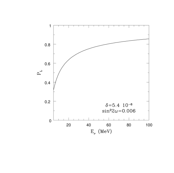
FIG. 4.: The Landau Zener jump probability $P_{L}$ at the lower resonance as a function of the neutrino energy for the small angle MSW solution (SMA) values of the mass squared difference and mixing angle $\omega$ for the 3-flavour case.

FIG. 5.: $\nu_{e}d$ event rates when the upper resonance is completely non-adiabatic. The solid lines represent the no-mixing case. The dotted and dashed lines are due to the effects of 3- and 4-flavour mixing. Results are shown for two different values of $\omega$ when $\epsilon=10^{-4}$.

FIG. 6.: $\overline{\nu}_{e}\,d$ event rates are shown as a function of positron energy, $E_{e}$. The solid lines represent the no-mixing case. The dotted and dashed lines are due to the effects of 3- and 4-flavour mixing. Results for two different values of $\omega$ are shown.

FIG. 7.: Total event rates (from combining the indivdual $\nu_{e}\,d$ and $\overline{\nu}_{e}\,d$ rates shown in Figs. 3 and 6) are shown as a function of the electron/positron energy, $E_{e}$, for two different values of $\omega$, and for $\epsilon=0.08$ so that the propagation is fully adiabatic. The dotted and dashed lines are due to the effects of 3- and 4-flavour mixing. Results from a 1 kton water detector (from $\overline{\nu}_{e}\,p$ alone) are shown on the right, for comparison.

FIG. 8.: Same as Fig. 7 but for $\epsilon\sim 0$ so that non-adiabatic effects are included. Hence this is a combination of Figs. 5 and 6.

FIG. 9.: The double ratio $R_{D/H}$ of the ratio of the total events observed through the detection of an electron (or positron) with $E_{e}\geq 5$ MeV, from a future supernova explosion to that expected, in a heavy water and a water detector, shown as a function of the (12) mixing angle $\omega$. Solid and dashed lines correspond to adiabatic ($\epsilon=0.08$) and non-adiabatic ($\epsilon\sim 0$) neutrino propagation at the upper resonance(s). The case for 3-flavour mixing is shown on the left and that for 4-flavours on the right. The vertical dotted lines indicate the currently favoured values of $\sin^{2}2\omega$ according to solar neutrino analysis.

FIG. 10.: The same as fig. 9, with a high energy cut on the electrons, $5<E_{e}<40$ MeV, to decrease sensitivity to the high energy tail of the neutrino spectrum.

FIG. 11.: The same as Fig. 3 for electron neutrinos in the no-mixing case (solid lines). Added are the dotted and dashed lines corresponding to the case when the supernova neutrino spectral temperatures are increased or decreased by 1 MeV in each time-bin.

FIG. 12.: The same as Fig. 6 for electron antineutrinos in the no-mixing case (solid lines). Added are the dotted and dashed lines corresponding to the case when the supernova neutrino spectral temperatures are increased or decreased by 1 MeV in each time-bin.

FIG. 13.: The same as fig. 9, but where the dashed curves now indicate the changes in the double ratio $R_{D/H}$ due to variations in temperature in the supernova model by $\pm 1$ MeV. The statistical errors are also plotted but are too small to be distinguished.

REFERENCES

- [1] IAU Circular No. 4316, 1987.
- [2] Kamiokande II Collaboration, K. Hirata et al., Phys. Rev. Lett. 58, 1490 (1987).
- [3] IMB Collaboration, R. M. Bionta et al., Phys. Rev. Lett. 58, 1494 (1987).
- [4] N. D. Hari Dass, D. Indumathi, A. S. Joshipura and M. V. N. Murthy, Curr. Sci. 56, 575 (1987).
- [5] J. Arafune and M. Fukugita, Phys. Rev. Lett. 5̱9, 367 (1987).
- [6] J. N. Bahcall and S. N. Glashow, Nature (London) 326, 476 (1987).
- [7] K. Sato and H. Suzuki, Phys. Rev. Lett. 58, 2722 (1987).
- [8] W. D. Arnett and J. L. Rosner, Phys. Rev. Lett. 58, 1906 (1987).
- [9] E.W. Kolb, A.J. Stebbins, and M.S. Turner, Phys. Rev. D 35, 3598 (1987).
- [10] R. Cowsik, Phys. Rev. D 37, 1685 (1988).
- [11] T. K. Kuo and J. Pantaleone, Phys. Rev. D37, 298 (1988).
- [12] Amol S.Dighe and Alexei Yu. Smirnov, Phys. Rev. D 62, 033007 (2000).
- [13] Shao-Hsuan Chiu and T. K. Kuo, Phys. Rev. D 61, 073015(2000)
- [14] J. F. Beacom and P. Vogel, Phys. Rev. D 58, 053010 (1998).
- [15] J. F. Beacom and P. Vogel, Phys. Rev. D58, 093012 (1998).
- [16] Sandhya Choubey and Kamales Kar, Phys. Lett. B 479, 402 (2000)
- [17] Petr Vogel, Invited talk at the 8th Int. Workshop on ”Neutrino Telescopes”, Venice Feb, 1999, astro-ph/9904338.
- [18] J. F. Beacom, Invited talk at the 23rd Johns Hopkins Workshop on Current Problems in Particle Theory, Neutrinos in the next millennium, Baltimore, June 1999. hep-ph/9909231.
- [19] Gautam Dutta, D. Indumathi, M.V.N. Murthy and G. Rajasekaran, Phys. Rev. D61, 013009 (2000).
- [20] Gautam Dutta, D. Indumathi, M.V.N. Murthy and G. Rajasekaran, Phys. Rev. D62, 093014 (2000).
- [21] C. Athanassopoulos, lsnd Collaboration, Phys. Rev. Lett. 81, 1774 (1998); Phys. Rev. C58, 2489 (1998).
- [22] W. C. Haxton, Phys. Rev. D 36, 2283 (1987).
- [23] Mohan Narayan, M. V. N. Murthy, G. Rajasekaran, and S. Uma Sankar, Phys. Rev. D 53, 2809 (1996); Mohan Narayan, G. Rajasekaran, and S. Uma Sankar, Phys. Rev. D 56, 437 (1997); S. Goswami, K. Kar, and A. Raychaudhuri, Int. J. Mod. Phys. A 12, 781 (1997); G. L. Fogli, E. Lisi, A. Marrone, and G. Scioscia, Phys. Rev. D59, 117303 (1999); ibid 033001; G. L. Fogli, E. Lisi, and D. Montanino, Astropart. Phys. 9, 119 (1998); G. L. Fogli, E. Lisi, D. Montanino, and G. Scioscia, Phys. Rev. D56, 4365 (1997).
- [24] M. Apollonio et al., chooz Collab., Phys. Lett. B 420, 397 (1998); Phys. Lett. B 466, 415 (1999) (hep-ex/9907037); Mohan Narayan, S. Uma Sankar, and G. Rajasekaran, Phys. Rev. D 58, 031301 (1998).
- [25] V. Barger, S. Pakvasa, T.J. Weiler, K. Whisnant, Phys. Rev. D 58, 093016 (1998) and references therein; S. Goswami, Phys. Rev. D 55, 2931 (1997) and references therein.
- [26] E. Ma, G. Rajasekaran, I. Stancu, Phys. Rev. D 61, 071302 (R) (2000).
- [27] O.L.G. Peres and A. Yu. Smirnov, preprint hep-ph/0011054, 2000.
- [28] Gautam Dutta, D. Indumathi, M.V.N. Murthy and G. Rajasekaran, Talk presented by DI at the XIV High Energy Physics Symposium, Hyderabad, India, 18–22 Dec, 2000; to be published.
- [29] L. Wolfenstein, Phys. Rev. D17, 2369 (1978); S. P. Mikheyev and A. Yu. Smirnov, Sov.J.Nucl.Phys, 42, 913 (1985); Nuovo Cimento, C9, 17(1986).
- [30] S.J. Parke, Phys. Rev. Lett. 57; See also the review by T. K. Kuo and J. Pantaleone, Rev. Mod. Phys. 61, 937 (1989).
- [31] T. Totani, K. Sato, H.E. Dalhed, J. R. Wilson, Astrophys. J. 496, 216 (1998); see also the references in [39] below.
- [32] J. N. Bahcall, Neutrino Astrophysics, Cambridge University Press, 1989.
- [33] K. Kubodera and S. Nozawa, Int. J. Mod. Phys. E3, 101 (1994).
- [34] P. Vogel and J. F. Beacom, Phys. Rev. D 60,053003 (1999).
- [35] S. Nakamura, T. Sato, V. Gudkov and K. Kubodera, preprint nucl-th/0009012, 2000.
- [36] M. Butler, J.-W. Chen, X. Kong, preprint nucl-th/0008032, 2000.
- [37] The Super Kamiokande Collab., S. Fukuda et al., preprint hep-ex/0103032.
- [38] The SNO Collab., A.B. Mc. Donald, Nucl. Phys. Proc. Suppl. 91, 21 (2000).
- [39] A. Burrows and J.M. Lattimer, Astrophys. J. 307, 107 (1986); R. Mayle, J. R. Wilson and D. N. Schramm, Astrophys. J. 318, 288 (1987).
- [40] J.N. Bahcall, P.I. Krastev, and A.Yu. Smirnov, Phys. Rev. D 58, 96016 (1998).
- [41] M.V. Garzelli and C. Giunti, preprint hep-ph/0012247, 2000, talk presented by C. Giunti at NOW 2000, Conca Specchiulla, Otranto, Italy, Sep 2000.
- [42] M.C. Gonzalez-Garcia, M. Maltoni, C. Pena-Garay and J.W.F. Valle, Phys. Rev. D63, 033005 (2001).
- [43] J.A. Pons, S. Reddy, M. Prakash, J.M. Lattimer, and J.A. Miralles, Astrophys. J. 513, 780 (1999).
- [44] K. Langanke, P. Vogel and E. Kolbe, Phys. Rev. Lett. 76, 2629 (1996).