Predictions for Neutrino Structure Functions
Abstract
The first measurements of are higher than current theoretical predictions. We investigate the sensitivity of these theoretical predictions upon a variety of factors including: renormalization scheme and scale, quark mass effects, higher twist, isospin violation, and PDF uncertainties.
1 Introduction
Deep inelastic lepton-nucleon scattering experiments have provided precision information about the quark distributions in the nucleon. However, there has been a long-standing discrepancy between the structure functions extracted from neutrino and muon experiments in the small range. Recently, a new analysis of differential cross sections and structure functions from CCFR -Fe and -Fe data was presented; in this study, the neutrino-muon difference is resolved by extracting the structure functions in a physics model independent way.[2]
In previous analyses of data,[3] structure functions were extracted by applying a slow rescaling correction to correct for the charm mass suppression in the final state. In addition, the term (used as input in the extraction) was calculated from a leading order charm production model. These resulted in physics model dependent (PMD) structure functions. In the new analysis,[2] slow rescaling corrections are not applied, and and were extracted from two parameter fits to the data.
The extracted physics model independent (PMI) values for are then compared with within the framework of NLO models for massive charm production; these are found to be in agreement, thus resolving the long-standing discrepancy between the two sets of data. However, the first measurements of are higher than current theoretical predictions. The objective of this paper is to investigate the sensitivity of upon a variety of factors including renormalization scheme and scale, quark mass effects, higher twist, isospin violation, and PDF uncertainties.

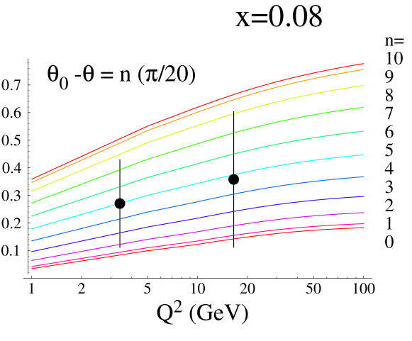
In Fig. 1 we have plotted the quantity for an isoscalar target computed to order . For comparison, we also display data from the CCFR analysis.[2] While there is much freedom in the theoretical calculation, the difference between these calculations and the data at low values warrants further investigation. We will discuss and compare the different theoretical calculations, and examine the inherent uncertainty in each with respect to different input parameters. We will also examine the experimental input, and assess uncertainties in this data.
1.1 Measurement of
The structure functions are defined in terms of the neutrino-nucleon cross section via:
| (1) |
where is the Fermi weak coupling constant, is the nucleon mass, is the incident energy, is the fractional energy transfer, and is the final state hadronic energy.
The sum of and differential cross sections for charged current interactions on an isoscalar target is then:
| (2) | |||||
where is the polarization of the virtual boson. In the above equation, we have used the relation:
| (3) |
where is the ratio of the cross-sections of longitudinally- to transversely-polarized -bosons, is the square of the four-momentum transfer to the nucleon, and is the Bjorken scaling variable. For , in neutrino scattering is expected to be somewhat larger than for muon scattering because of the production of massive charm quarks in the final state for the charged current neutrino production.
Using Eq. (2) and Eq. (3), and can be extracted separately. Because of the positive correlation between and , the extracted values of are rather insensitive to the input . If a large input is used, a larger value of is extracted from the distribution, thus yielding the same value of . In contrast, the extracted values of are sensitive to the assumed value of , which yields a larger systematic error, shown on the data. For the QCD-inspired fit in [4] is used, but corrected for charged current neutrino scattering using a leading order slow rescaling model. This gives precisely the same type of correction as a full NLO calculation including the massive charm quark, as shown in Ref. [5], but leads to a somewhat higher normalization than the perturbative correction. It is arguable which prescription for leads to the better fit to existing data, but the difference between the two leads to an uncertainty in of the order of the systematic error shown. Clearly a further reduction in the assumed value of R (even down to zero), as suggested by models including resummations, would still leave a discrepancy between the lowest data points and the theoretical predictions.
1.2 Quark Parton Model Relations
Now that we have outlined the experimental method used in the extraction of the structure functions, it is instructive to recall the simple leading-order correspondence between the ’s and the PDF’s:000To exhibit the basic structure, the above is taken in the limit of 4 quarks, a symmetric sea, and a vanishing Cabibbo angle. Of course, the actual analysis takes into account the full structure.[2]
| (4) |
Therefore, the combination yields:
| (5) |
Note that since this quantity involves the parity violating structure function , this measurement has no analogue in the neutral current photon-exchange process. Also note that since, at leading-order, is directly sensitive to the strange and charm distributions, this observable can be used to probe the heavy quark PDF’s, and to understand heavy quark (charm) production. We discuss these possibilities further in the following subsection.
1.3 Implications for PDF’s
We have illustrated in Eq. (5) how is closely tied to the heavy quark PDF’s. The questions is: given the present knowledge base, should we use to determine the heavy quark PDF’S, or vice verse. To answer this question, we briefly review present measurements of heavy quark PDF’s, and assess their uncertainty.
1.3.1 Tevatron Production
The precise measurement of plus heavy quark events provides important information on heavy quark PDF’s; additionally, such signals are a background for Higgs and squark searches.[6, 7]
Unfortunately, a primary uncertainty for production comes from the heavy quark PDF’s. Given that is sensitive to these heavy quark PDF’s, we see at least two scenarios. One possibility is that new analysis of present data will resolve this situation prior to Run II, and provide precise distributions as an input to the Tevatron data analysis. If the situation remains unresolved, then new data from Run II may help to finally solve this puzzle. In the far future, a neutrino experiment from the neutrino factory at a linear collider would be an ideal tool to measure any neutrino structure function.[8]
1.3.2 DIS Di-muon production
The strange distribution is directly measured by dimuon production in neutrino-nucleon scattering.111Presently, there are a number of LO analyses, and one NLO ACOT analysis.[9, 10, 11, 12]. Results of a recent LO analysis by NOMAD [13] are in line with these experiments. The basic sub-process is with a subsequent charm decay .
DIS dimuon measurements have safely established the breaking of the flavor symmetry,
| (6) |
in the nucleon sea. Still, there remain large uncertainties for the -quark distribution in the kinematic regions relevant for , even though the -range of the CCFR dimuon measurements [10, 14] is comparable. CCFR recorded 5044 and 1062 events with , , , and . The more recent NuTeV experiment recorded a similar sample of events, and these are presently being analysed through a MC simulation based on NLO quark- and gluon-initiated corrections at differential level[11, 15, 16]. A complete NLO analysis of this data together with a global analysis may help to further constraint the strange quark distribution.
At present, PDF sets take strangeness suppresssion into account by imposing the constraint in Eq. (6) as at the PDF input scale , [17, 18] or by evolving from a vanishing input at a lower scale.[19] The residual uncertainty can be large, as can be seen from the collection of strange seas in Fig. 2.

1.3.3 Charged and Neutral Current DIS
The strange distribution can also be extracted indirectly using a combination of charged () and neutral () current structure functions; however, the systematic uncertainties involved in this procedure make an accurate determination difficult.[2] The basic idea is to use the (leading-order) relation
| (7) |
to extract the strange distribution. Here, represents a sum over all quark flavors. This method is complicated by a number of issues including the component which can play a crucial role in the small- region—precisely the region where we observe the discrepancy. From the corresponding relation:
| (8) |
we see that these problems are not independent; however, this information, together with the exclusive dimuon events, may provide a more precise determination of the strange quark sea, and help to resolve our puzzle.
Prior to the DIS dimuon data, the 1992 CTEQ1 analysis [20] found that a combination of NC structure functions from NMC[21] and the physics-model-dependent charged current structure functions from CCFR [10] seem compatible with approximate -symmetry, i.e., in Eq. (6). Recent dimuon measurements now exclude an -symmetry .
We shall explore the effect of on in Sec. [3.2].
2 Dependence of on input parameters
We now systematically investigate the sensitivity of the theoretical predictions of upon a variety of factors including: renormalization scheme and scale, quark mass effects, higher twist, isospin violation, and PDF uncertainties.
To simplify this analysis, we first examine the influence of these factors on the LO expression: ; after using this as a “toy model,” we will then return to the full NLO calculation in the next section.222Note that a possible asymmetry [22] would average out in . For most variables, the simplified LO is sufficient to display the general behavior of the full NLO result. There are two exceptions: 1) the scheme dependence, and 2) the PDF dependence. These factors depend on the interplay of both the quark-initiated LO contributions as well as the NLO gluon-initiated contributions. For this reason, we will postpone discussion of these effects until the following section.
2.1 Charm Mass
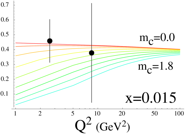
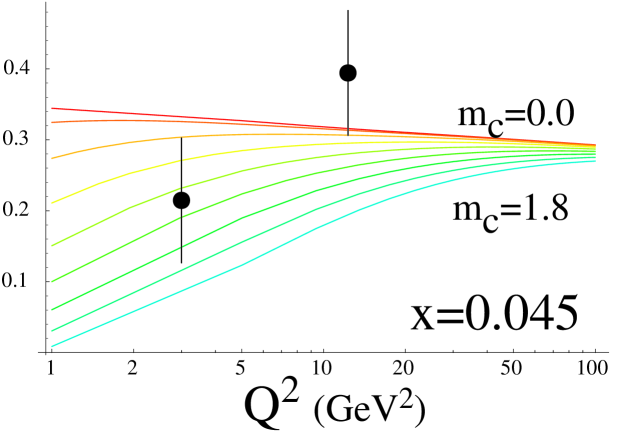
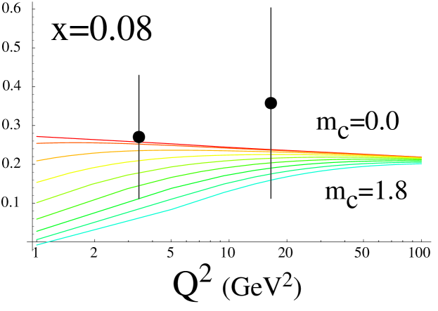
We start by examining the effect of the charm mass, , on . In Fig. 3, we plot the leading-order expression vs. for values of in the range GeV using steps of 0.2 GeV. Here, we define which is a “slow-rescaling” type of correction[23, 24] which (crudely) includes mass effects by shifting the variable. “Slow rescaling” naturally arises at LO from the single-charm threshold condition() and is required at NLO for consistent mass factorization [24, 25].
Note, the result of this correction is most significant at low . To isolate the kinematic dependence, we have chosen the scale . (We will separately vary the scale in the following subsection.)
Note that this exercise is only altering the charm mass in one aspect of the calculation; to be entirely consistent it would be necessary to obtain parton distributions (particularly the charm quark) using fits with different charm masses. For charm masses in the range 1.2 to 1.8 GeV, this will be a small effect; for charm masses below GeV, (which is below the experimentally allowed range[26, 27]), such issues become important and the curves of Fig. 3 will be modified, i.e. lower will lead to longer evolution for charm, a larger charm distribution, and a lowering of the curves in Fig. 3.
While taking does raise the theoretical curves in the regions where we observe the discrepancy (namely, the low region), varying even within the wide range of GeV (lower 4 curves) does not give us sufficient flexibility to match either the shape or normalization of the data.
2.2 Scale
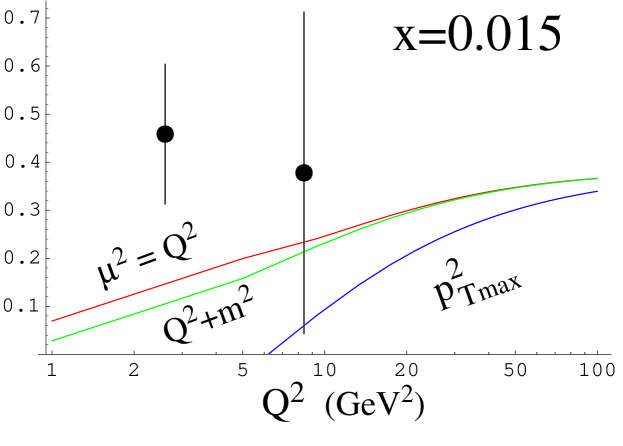
Next, we investigate the variation of with the renormalization/factorization scale . We use three choices of the scale:
-
•
,
-
•
,
-
•
.
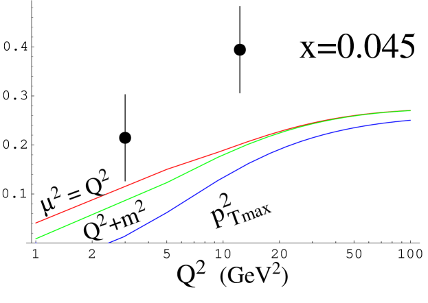
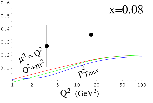
Of course, with scales of and differ only at lower values of ; with scale of is comparable to and at larger , but lies below for smaller . The scale choice leads to an improvment over by providing a lower bound on to keep the scale in the perturbative region.
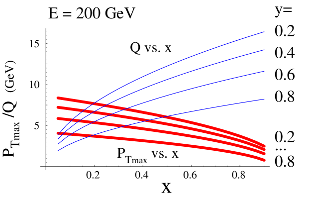
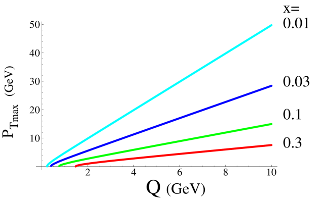
The choice of is motivated, in part, by some observations by Collins.[28] To display the relationship between and , in Fig. 5 we plot both and vs. for 4 choices of ; note[14] that the -dependence of is opposite that of . While tying the scale choice of to has some interesting intuitive interpretations,333Technically, the interpretation is in terms of the characteristic of the partonic subprocess, but this is unobservable; therefore is used instead.[28] for small this scale clearly becomes too large for the relevant physics. In any case, it cannot help us with our problem as the scale choice of moves the theory curves away from the data.
2.3 Higher Twist

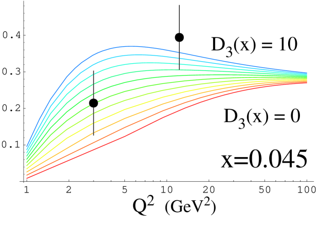
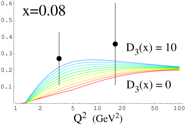
We now illustrate the potential effects due to higher twist contributions. We parameterize such contributions by multiplying the leading-twist terms by a correction factor that will increase at low . More specifically we use:[29]
| (9) |
where . We vary over the range [0,10] in steps of . (For the purposes of our simple illustration, it is sufficient to take to be independent of .) We will find that this range is well beyond what is allowed by experiment; however, we display this exaggerated range to make the effect of the higher twist contributions evident.
To normalize this choice with the allowable range consistent with data, we compare with the MRST higher twist fit which extracted a limit on the function . We see from the table of that the allowed contribution from the higher twist terms is quite small. In addition, we note that the sign for obtained for the relevant small- region tends to be negative–exactly the opposite sign that is needed to move the theory toward the data.
As we have shown constraints on , the obvious question is should we expect to be substantially different? A calculation of the power corrections using renormalons[30] suggests that while both and are of the same order of magnitude as and have similar -dependence, that and are even more negative than ; again, this trend would move the theory farther from the data. Therefore, we conclude that that represents a conservative limit for the power corrections.
Examining Fig. 6, we note that it would take an enormous higher twist contribution to bring the normalization of the curves in the range of the data points, and still the shape of the -dependence is not well matched; hence, we conclude that this is not a compelling solution.
| LO | NLO | NNLO | |
|---|---|---|---|
| 0 – 0.0005 | 0.4754 | 0.0116 | 0.0061 |
| 0.0005 – 0.005 | 0.2512 | 0.0475 | 0.0437 |
| 0.005 – 0.01 | 0.2481 | 0.1376 | 0.0048 |
| 0.01 – 0.06 | 0.2306 | 0.1271 | 0.0359 |
| 0.06 – 0.1 | 0.1373 | 0.0321 | 0.0167 |
| 0.1 – 0.2 | 0.1263 | 0.0361 | 0.0075 |
| 0.2 – 0.3 | 0.1210 | 0.0893 | 0.0201 |
| 0.3 – 0.4 | 0.0909 | 0.1710 | 0.1170 |
| 0.4 – 0.5 | 0.1788 | 0.0804 | 0.0782 |
| 0.5 – 0.6 | 0.8329 | 0.3056 | 0.1936 |
| 0.6 – 0.7 | 2.544 | 1.621 | 1.263 |
| 0.7 – 0.8 | 6.914 | 5.468 | 4.557 |
| 0.8 – 0.9 | 19.92 | 18.03 | 15.38 |
2.4 Isospin Violations
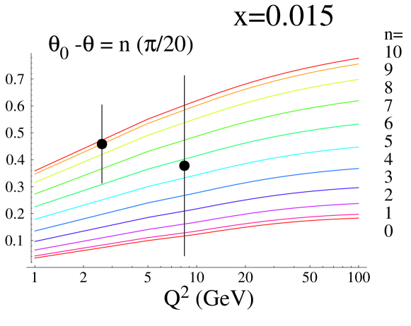
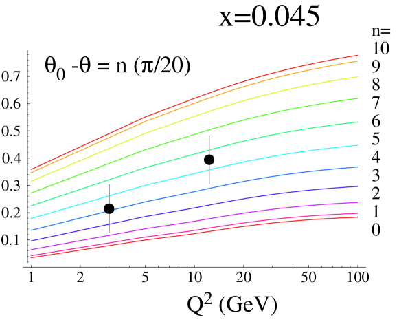
The naive parton model identity in Eq. (5) is modified if the full (non-diagonal) CKM structure, NLO QCD radiative corrections, and QCD based charm production are taken into account. This expression is also modified even in leading-order if we have a violation of exact isospin-symmetry, (or charge symmetry); e.g., . In deriving Eq. (5), isospin-symmetry was necessary to guarantee that the -contributions cancel out in the difference, thereby leaving only the and contributions.444Note we have not investigated shadowing corrections. The CCFR data on Fe is converted with an isoscalar correction, and the corresponding uncertainties are included in the data.[3]
The validity of exact charge symmetry (CS) has recently been reexamined.[32] Residual -contributions to from charge symmetry violation (CSV) would be amplified due to enhanced valence components , and because the transitions are not subject to slow-rescaling corrections which strongly suppress the contribution to , as illustrated in Fig. 3.
We will examine possible contributions to by considering a “toy” model to parameterize the CS-violations. In isospin space, we can parameterize a general transformation as a rotation:
| (10) |
where is a rotation matrix, and is the normalization factor. For example, in this model the -distribution in the neutron would be related to the proton distributions via the relation:
| (11) |
For , we recover the symmetric limit . Note that we define the normalization such that this model preserves the sum rule:
| (12) |
Note that Eq. (10) should not be considered a serious theory,555E.g., it does strictly speaking not commute with evolution. but rather a simple one-parameter () model which is flexible enough to illustrate a range of CSV effects for .
In Fig. 7 we vary over the its maximum range in steps of . The exact charge symmetry limit () of Eq. (2.4) corresponds to the lowest curve in Fig. 7. Note the effect of the CSV contribution monotonically increases as deviates from the charge symmetry (CS) limit . From the plot we observe that a violation of is required to bring the theory in the neighborhood of the data.
At the relevant values of interest for , this translates (via Eq. (2.4) and its analogue for ) into a symmetry violation for , and a symmetry violation for . Specifically,
| (13) | |||||
| (14) |
Since the electroweak couplings are flavor-independent, (), is in principle insensitive to a re-shuffling of the CSV contributions between and . In particular, if we define the shift due to CSV in as , we find:
| (15) |
where
| (16) |
The expression for of Eq. (15) is evaluated at from Eq. (2.4) with and is plotted in Fig. 8.666 Again, the detailed -shape from Eq. (2.4) should not be taken as a serious model prediction.
Although this level of isospin violation certainly improves the description of , it is necessary to consider precisely what level of violation is actually allowed by other experimental data. For instance, it has previously been suggested that the discrepancy between from neutrino and muon data itself may be due to isospin violation.[32] This type of violation required that be very different to in the region of interest.
The measurement of the lepton charge asymmetry in W decays from the Tevatron [33, 34] places tight constraints on the up and down quark distributions in the range , constraining them to be approximately as specified in the parton sets obtained by the global analyses. While only strictly telling us about parton distributions in the proton, this data rules out an isospin violation of this type to about as demonstrated in [34].
However, there are other strong constraints on isospin violation. For example, we note that while the toy model above leaves the neutron singlet combination invariant at the level in the region , it would lower the NC observable:
| (17) |
by about 10%. An effect of this size would definitely be visible in NMC data which has an uncertainty of order a few percent in this kinematic region, and acts as a major constraint.[21]
At this point, one could play clever games to evade the constraints of specific experiments. For example, a re-shuffling of CSV contributions between the individual in Eq. (15) according to:
would keep Eq. (17) invariant. However, this would in turn raise the CC observable Eq. (15) by ; though it would help to explain the excess in , it would spoil the new-found compatibility between neutral current and charged current data.
In addition, there are also fixed-target Drell-Yan experiments[35, 36] such as NA51 and E866 which precisely measure in the range[36] , and are also sensitive to isospin violating effects.
We therefore conclude that the many precise data sets which constrain different combinations of the PDF’s probably leave no room for CSV contributions of the magnitude necessary to fully align the theory curves with the data. However, we should add the caveat that an exhaustive investigation of the interplay of these different data sets and their influence on will only be possible within a global PDF analysis
3 NLO calculation of
Now that we have used the leading-order expression for to systematically investigate dependence of this observable on various parameters, in this section we now turn to the full NLO calculation.
3.1 Contributions to the NLO Calculation

In Fig. 9, we have plotted the LO and NLO calculations for vs. on an isoscalar target in 3 and 4 flavor schemes. The 3-flavor LO calculation (f=3, ) involves primarily the strange quark contribution, , as the charm distribution is excluded in this case. When the higher order terms are included (f=3, ), this result moves (substantially) toward the predictions of the 4-flavor scheme. We note that while the 3-flavor LO calculation (f=3, ) appears consistent with the data, we cannot take this result as a precise theoretical prediction as this simplistic result is highly dependent on scheme and scale choices; a result that is verified by the large shift in going from LO to NLO.
The pair of curves in the 4-flavor scheme (using the CTEQ4HQ distributions) nicely illustrates how the charm distribution evolves as for increasing ; note, enters with a negative sign so that the 4-flavor result is below the 3-flavor curve. For the scale choice, we take . While the scale choice is useful for instructive purposes such as demonstrating the matching of the 3- and 4-flavor calculations at , the choice is more practical as it provides a lower bound on which is important for the PDF’s and . (Cf., Sec. [3.3], and Ref. [37].)
Additionally we note the stability of the 4-flavor scheme in contrast to the 3-flavor scheme. The shift of the curves when including the NLO contributions is quite minimal, particularly when compared with the 3-flavor result.[38, 39] This suggests that organizing the calculation to include the charm quark as a proton constituent can be advantageous even at relatively low values of the energy scale.
3.2 PDF Uncertainties: s(x), …

In Fig. 10, we show the variation of NLO calculation of on the strange-quark PDF. To obtain a realistic assessment of the dependence, we have use the NLO calculation with PDF’s based on the MRST set which are re-fit with the value of constrained to be . Note, by re-fitting the PDF’s with the chosen value of we are assured to have an internally consistent set of PDF’s with appropriate matching between the quarks and gluon, and with the sum-rules satisfied.777Note, is certainly -dependent, and the values for quoted above correspond to the of the evolution. While compares the integral of to the seq-quarks, there is also the possibility of an -dependent variation. This has been studied in the fits of the strange-sea[10, 14, 11, 40]; we shall find that such subtle effects can play no role in resolving the issue.
| Experiment | Order | Ref. | |
|---|---|---|---|
| CDHS | LO | [9] | |
| FMMF | LO | [41] | |
| CHARM II | LO | [12] | |
| CCFR∗ | NLO | [14] | |
| CCFR† | NLO | [14] | |
| CCFR† | LO | [10] | |
| NOMAD | LO | [13] | |
| NuTeV | LO | [11] |
∗Collins-Spiller Fragmentation.
† Peterson Fragmentation.
The choice is in line with the many experimental determinations of , cf., Table. 2; as expected, this prediction lies farthest from the data points.
The choice is taken as an extreme upper limit given the experimental constraints; actually, in light of the results of Table. 2, this is arguably beyond present experimental bounds. This prediction is marginally consistent at the outer reach of the systematic + statistical error bars.
Finally, we take an symmetric set () purely for illustrative purposes. It is interesting to note that even this extreme value is still below the central value of the data points at the higher values.
In conclusion we note that increasing the strange quark distribution does succeed in moving the theory toward the data; however, our consistent NLO analysis presented here suggests that the we have only limited freedom to increase , and that this alone is not sufficient to obtain good agreement between theory and data.
3.3 Scheme Choice

In our final section, we present the best theoretical predictions presently available to demonstrate the scheme dependence of . Specifically, in Fig. 11 we show predictions for:
All these calculations use NLO matrix elements, and are matched with appropriate global PDF’s which are fitted in the proper scheme.
The first observation we make is how closely these four predictions match, especially given the wide variation displayed in previous plots such as Fig. 9. In hindsight, this result is simply a consequence of the fact that while different renormalization schemes can produce different results, this difference can only be higher order.888To be precise, different renormalization schemes can differ by i) terms of higher order in the perturbation series, and ii) terms of higher twist which do not factorize.[45, 46] Thus, the difference between these curves is indicative of terms of order which have yet to be calculated.999For asymptotic results at order , see Ref. [38]. When terms of order are included, the span of these predictions will be systematically reduced to order .
In Fig. 11, we note the very close agreement among the VFS calculations, particularly the TR calculation and the ACOT calculation with CTEQ4 PDF’s. The ACOT calculation with the two CTEQ curves show primarily the effect of the charm distribution, as CTEQ4 uses and CTEQ5 uses . The GRV calculation shows the effect of using yet a different scheme, in this case a FFN scheme, with its appropriately matched PDF. Were we to use MRST or CTEQ PDF’s, the spread of these theory curves would decrease; however, this would most likely represent an underestimate of the true theoretical uncertainties arising from both the hard cross section and PDF’s.101010The computation of PDF errors is a complex subject. For some recent approaches to this topic see: Refs.[17, 18, 47, 40].
While we consider it a triumph of QCD that different schemes truly yield comparable results (higher order terms aside), we should be cautious and note that the spread of these curves can only underestimate the true theoretical uncertainty. Note that GRV has a rather different strange distribution due to a different philosophy of obtaining this distribution rather than due to a different scheme.
4 Conclusions and Outlook
Comprehensive analysis of the neutrino data sets can provide incisive tests of the theoretical methods, particularly in the low regime, and enable precise predictions that will facilitate new particle searches by constraining the PDF’s. This document serves as a progress report, and work on these topics will continue in the future.
Theoretical predictions for undershoot preliminary fixed target data at the -level at low and . The neutrino structure function is obviously sensitive[48] to the strange sea of the nucleon and the details of deep inelastic charm production. A closer inspection reveals, however, considerable dependence upon factors such as the charm mass, factorization scale, higher twists, contributions from longitudinal polarization states, nuclear shadowing, charge symmetry violation, and the PDF’s. This makes an excellent tool to probe both perturbative and non-perturbative QCD.
We have explored the variation of on the above factors and found none of these to be capable of resolving the discrepancy between the data and theory.
Although we have not eliminated the possibility that the entire set of parameters conspires to align the theory with the data, we have demonstrated this to be extremely unlikely. Of course, a definitive answer can only be obtained by a global analysis which combines the neutrino data for dimuons, , , and .
As the situation stands now, this puzzle poses an important challenge to our understanding of QCD and the related nuclear processes in an important kinematic region. The resolution of this puzzle is important for future data analysis, and the solution is sure to be enlightening, and allow us to expand the applicable regime of the QCD theory.
Acknowledgments
This work is supported by the Royal Society, the U.S. Department of Energy, the National Science Foundation, the Lightner-Sams Foundation, and the ‘Bundesministerium für Bildung, Wissenschaft, Forschung und Technologie’, Bonn.
We thank J. Bluemlein, A. Bodek, J. Conrad, J. Morfin, S. Kuhlmann, R.G. Roberts, H. Schellman, M. Shaevitz, J. Smith, and W.-K. Tung, for valuable discussions.
References
- [1]
- [2] U. K. Yang et al. [CCFR-NuTeV Collaboration], hep-ex/0009041.
-
[3]
W. G. Seligman et al., CCFR Collab.,
Phys. Rev. Lett. 79, 1213 (1997);
W. G. Seligman, Ph.D. Thesis, Columbia University, Nevis-292 (1997). - [4] L. W. Whitlow, E. M. Riordan, S. Dasu, S. Rock and A. Bodek, Phys. Lett. B282, 475 (1992).
- [5] C. Boros, F.M. Steffens, J.T. Londergan and A.W. Thomas, Phys. Lett. B468, 161 (1999).
- [6] W. T. Giele, S. Keller and E. Laenen, Nucl. Phys. Proc. Suppl. 51C, 255 (1996); Phys. Lett. B372, 141 (1996); hep-ph/9408325.
- [7] R. Demina et al., hep-ph/0005112. L. de Barbaro et al., hep-ph/0006300.
- [8] R.D. Ball, D.A. Harris, and K.S. McFarland, hep-ph/0009223.
- [9] H. Abramowicz et al., CDHSW Collab., Z. Phys. C15, 19 (1982).
- [10] S.A. Rabinowitz et al., CCFR Collab., Phys. Rev. Lett. 70, 134 (1993).
- [11] T. Adams et al. [NuTeV Collaboration], hep-ex/9906037.
- [12] P. Vilain et al. [CHARM II Collaboration], Eur. Phys. J. C11, 19 (1999).
- [13] P. Astier et al. [NOMAD Collaboration], Phys. Lett. B486 (1900) 35.
- [14] A. O. Bazarko et al. [CCFR Collaboration], Z. Phys. C65, 189 (1995); A. O. Bazarko, Ph.D. Thesis. NEVIS-1504
- [15] M. Glück, S. Kretzer and E. Reya, Phys. Lett. B398, 381 (1997); B405, 392 (1997) (E).
- [16] S. Kretzer and F. Olness, in preparation.
- [17] A.D. Martin, R.G. Roberts, W.J. Stirling, R.S. Thorne, Eur. Phys. J. C14, 133 (2000).
- [18] H. L. Lai et al., Eur. Phys. J. C12, 375 (2000).
- [19] M. Gluck, E. Reya and A. Vogt, Eur. Phys. J. C5, 461 (1998).
- [20] J. Botts et al., CTEQ1, Phys. Lett. B304, 159 (1993).
- [21] NMCollaboration: M. Arneodo et al., Nucl. Phys. B483, 3 (1997).
- [22] S.J. Brodsky and B.-Q. Ma, Phys. Lett. B381, 317 (1996).
- [23] R.M. Barnett, Phys. Rev. Lett. 36, 1163 (1976); H. Georgi and H.D. Politzer, Phys. Rev. D14, 1829 (1976).
- [24] F. Olness, W.K. Tung, Nucl. Phys. B308 (1988) 813; M. Aivazis, F. Olness, W.K. Tung, Phys. Rev. D50 (1994) 3085; M. Aivazis, J.C. Collins, F. Olness, W.K. Tung, Phys. Rev. D50 (1994) 3102.
- [25] T. Gottschalk, Phys. Rev. D23, 56 (1981); M. Glück, S. Kretzer and E. Reya, Phys. Lett. B380, 171 (1996); B405, 391 (1996) (E).
- [26] J. Breitweg et al. [ZEUS Collaboration], Eur. Phys. J. C12, 35 (2000); C. Coldewey [H1 and ZEUS Collaborations], Nucl. Phys. Proc. Suppl. 74, 209 (1999).
- [27] D.E. Groom et al., The European Physical Journal 15 (2000) 1, available on the PDG WWW pages (URL: http://pdg.lbl.gov/).
- [28] J. C. Collins, ANL-HEP-CP-90-58 Proc. of 25th Rencontre de Moriond: High Energy Hadronic Interactions, Les Arcs, France, Mar 11-17, 1990.
- [29] A. D. Martin, R. G. Roberts, W. J. Stirling and R. S. Thorne, Phys. Lett. B443, 301 (1998).
- [30] M. Dasgupta and B. R. Webber, Phys. Lett. B382, 273 (1996).
- [31] A. D. Martin, R. G. Roberts, W. J. Stirling and R. S. Thorne, Eur. Phys. J. C18, 117 (2000).
- [32] C. Boros, F.M. Steffens, J.T. Londergan and A.W. Thomas, Phys. Lett. B468, 161 (1999); C. Boros, J.T. Londergan, A.W. Thomas, Phys. Rev. D59, 074021 (1999); C. Boros, J.T. Londergan, A.W. Thomas, Phys. Rev. Lett. 81, 4075 (1998) and related references therein.
- [33] F. Abe et al. [CDF Collaboration], Phys. Rev. Lett. 81, 5754 (1998).
- [34] A. Bodek, Q. Fan, M. Lancaster, K.S. McFarland and U.K. Yang, Phys. Rev. Lett. 83, 2892 (1999).
- [35] A. Baldit et al. [NA51 Collaboration], Phys. Lett. B332, 244 (1994).
- [36] E. A. Hawker et al. [FNAL E866/NuSea Collaboration], Phys. Rev. Lett. 80 (1998) 3715.
- [37] C. Schmidt, hep-ph/9706496; J. Amundson, C. Schmidt, W. K. Tung, X. Wang, JHEP0010, 031 (2000); J. Amundson, F. Olness, C. Schmidt, W. K. Tung, X. Wang, FERMILAB-CONF-98-153-T, Jul 1998.
- [38] M. Buza and W.L. van Neerven, NPB 500, 301 (1997). M. Buza, Y. Matiounine, J. Smith, R. Migneron and W. L. van Neerven, Nucl. Phys. B472, 611 (1996).
- [39] A. Chuvakin, J. Smith, W.L. van Neerven, Phys. Rev. D 61, 096004 (2000); Phys. Rev. D 62, 036004 (2000); A. Chuvakin, J. Smith, hep-ph/9911504.
- [40] V. Barone, C. Pascaud and F. Zomer, Eur. Phys. J. C12, 243 (2000).
- [41] B. Strongin et al., Phys. Rev. D43, 2778 (1991).
- [42] R.S. Thorne, R.G. Roberts, hep-ph/0010344; Phys. Rev. D57 (1998) 6871.
- [43] S. Kretzer, I. Schienbein Phys. Rev. D56 (1997) 1804; Phys. Rev. D58 (1998) 094035; Phys. Rev. D59 (1999) 054004.
- [44] H. L. Lai et al., Phys. Rev. D55 (1997) 1280.
- [45] J.C. Collins, W.-K. Tung Nucl. Phys. B278, 934 (1986); J.C. Collins, Phys. Rev. D58 (1998) 094002.
- [46] M. Krämer, F. Olness, D. Soper, Phys. Rev. D 62, 096007 (2000);
- [47] S. Alekhin, Eur. Phys. J. C10, 395 (1999); W. T. Giele and S. Keller, Phys. Rev. D 58, 094023 (1998); W. T. Giele, S. Keller and D. A. Kosower, “Parton distributions with errors,” In *La Thuile 1999, Results and perspectives in particle physics* 255-261; J. Pumplin, D. R. Stump and W. K. Tung, hep-ph/0008191.
- [48] V. Barone, U. D’Alesio and M. Genovese, Phys. Lett. B357, 435 (1995).