Relativistic Many-Body Hamiltonian Approach to Mesons

Abstract

We represent QCD at the hadronic scale by means of an effective Hamiltonian, $H$, formulated in the Coulomb gauge. As in the Nambu-Jona-Lasinio model, chiral symmetry is explicity broken, however our approach is renormalizable and also includes confinement through a linear potential with slope specified by lattice gauge theory. This interaction generates an infrared integrable singularity and we detail the computationally intensive procedure necessary for numerical solution. We focus upon applications for the $u,d,s$ and $c$ quark flavors and compute the mass spectrum for the pseudoscalar, scalar and vector mesons. We also perform a comparative study of alternative many-body techniques for approximately diagonalizing $H$: BCS for the vacuum ground state; TDA and RPA for the excited hadron states. The Dirac structure of the field theoretical Hamiltonian naturally generates spin-dependent interactions, including tensor, spin-orbit and hyperfine, and we clarify the degree of level splitting due to both spin and chiral symmetry effects. Significantly, we find that roughly two-thirds of the $\pi$-$\rho$ mass difference is due to chiral symmetry and that only the RPA preserves chiral symmetry. We also document how hadronic mass scales are generated by chiral symmetry breaking in the model vacuum. In addition to the vacuum condensates, we compute meson decay constants and detail the Nambu-Goldstone realization of chiral symmetry by numerically verifying the Gell-Mann-Oaks-Renner relation. Finally, by including D waves in our charmonium calculation we have resolved the anomalous overpopulation of $J/\Psi$ states relative to observation.
PAC number(s): 12.39.Pn, 12.40.Yx

I Introduction

In a series of publications [1, 2, 3, 4] an ambitious QCD program has been initiated to comprehensively investigate hadron structure. The theoretical formulation entails renormalization and utilizes established many-body techniques to approximately diagonalize an effective confining Hamiltonian. This paper, a detailed continuation of our recent letter [3], focuses upon the quark sector and reports numerical results for mesons complementing our previous gluon study [1].

Over the years there have been many meson investigations, from the early, simple non-relativistic constituent quark model calculations to more involved relativistic, field theoretical approaches implementing current quarks and spontaneous chiral symmetry breaking. A common shortcoming of these analyses is an inability to consistently reproduce the physical mass spectrum of the scalar and pseudoscalar mesons. Our paper addresses this issue and significantly extends the pioneering work of the Orsay group [5], Adler and Davis [6], and the Lisbon investigators [7]. In our approach the exact QCD Hamiltonian in the Coulomb gauge is modeled by an effective, confining Hamiltonian, $H$, that is fully relativistic with quark field operators and current quark masses. However, before approximately diagonalizing $H$, a similarity transformation is implemented to a new quasiparticle basis having a dressed, but unknown constituent mass. As described in Sec. II, this transformation entails a rotation which mixes the bare quark creation and annihilation operators. By then performing a variational calculation to minimize the ground state (vacuum) energy, a specific angle and corresponding quasiparticle mass is selected. In this fashion chiral symmetry is dynamically broken and a non-trivial vacuum with quark condensates emerges. This treatment is precisely analogous to the Bardeen, Cooper, and Schrieffer (BCS) description of a superconducting metal as a coherent vacuum state of interacting quasiparticles combining to form condensates (Cooper pairs). Excited states (mesons) can then be represented as quasiparticle excitations using standard many-body techniques which in this work will be the Tamm-Dancoff (TDA) and random phase approximation (RPA) methods. The two treatments are truncated at the one quasiparticle, one quasihole level and then numerically compared. Our RPA analysis confirms and extends the early work of Ref. [8] which utilized an extended Nambu-Jona-Lasinio mean field approach.

Two other comments are in order before proceeding. First, there are several reasons for choosing the Coulomb gauge framework. As discussed by Zwanziger [9], the Hamiltonian is renormalizable in this gauge and, equally as important, the Gribov problem (${\bf\nabla}\cdot{\bf A}=0$ does not uniquely specify the gauge) can be resolved (see Refs. [2, 9] for further discussion). Related, there are no spurious gluon degrees of freedom since only transverse gluons enter. This ensures all Hilbert vectors have positive normalizations which is essential for using variational techniques that have been widely successful in atomic, molecular and condensed matter physics. Second, due to Fock space truncations our analysis is not Lorentz invariant. However, we only plan to use one frame and do not compute hadron form factors with this method. Interestingly, violating Lorentz non-invariance implies a prefered reference frame, which, as selected by chiral symmetry breaking, is the condensate rest frame.

This paper consists of six sections and two appendices. The next section introduces our effective, QCD inspired Hamiltionian and developes the BCS vacuum treatment leading to the quasiparticle mass gap equation. We also compare our approach to the classic Nambu-Jona-Lasinio model. In Sec. III we detail our numerical, supercomputer solution of the gap equation along with the quark condensate and constituent mass values. Sections IV A and IV B describe the TDA and RPA, respectively, while Sec. IV C addresses weak decays and Sec IV D presents a derivation of the Gell-Mann-Oakes-Renner relation. The TDA and RPA meson spectra are compared and discussed in Sec. V. This section also includes results from a simple $SU_{f}(3)$ flavor mixing analysis for the $\eta$-$\eta^{\prime}$ system and our predictions for the charmed mesons. Conclusions and future work are summarized in Sec. VI. Finally, Appendix A provides further details regarding the BCS transformation and vacuum state while Appendix B presents the most general TDA equation for arbitrary angular momentum.

II Hamiltonian and mass gap equation

A Effective Hamiltonian

By introducing a phenomenological confining potential, $V_{L}$, the QCD Coulomb gauge Hamiltonian [2] for the quark sector can be replaced by an effective Hamiltonian

$$H=\int d\vec{x}\Psi^{\dagger}(\vec{x})(-i\vec{\alpha}\cdot\vec{\nabla}+\beta m)\Psi(\vec{x})-\frac{1}{2}\int d\vec{x}d\vec{y}\rho^{a}(\vec{x})V_{L}(\arrowvert\vec{x}-\vec{y}\arrowvert)\rho^{a}(\vec{y})$$ (1)

where $\Psi$, $m$ and $\rho^{a}(\vec{x})=\Psi^{\dagger}(\vec{x})T^{a}\Psi(\vec{x})$ are the current (bare) quark field, mass and color density, respectively (for a more complete discussion, especially for the heavy quark sector, consult Refs. [9, 10]). For notational ease the flavor subscript is omitted (same $H$ for each flavor) and the color index runs $a=1...8$. Motivated by lattice gauge studies we adopt a linear confining interaction, $V_{L}=\sigma\arrowvert\vec{x}-\vec{y}\arrowvert$, with slope $\sigma=.18$ $GeV^{2}$ also specified by lattice and Regge phenomenology. In our analysis we have also performed calculations with and without the leading QCD canonical or Coulomb (one-gluon exchange) interaction, $V_{C}=-\frac{\alpha_{s}}{\arrowvert\vec{x}-\vec{y}\arrowvert}$, with $\alpha_{s}=\frac{g^{2}}{4\pi}$ $\cong$ $.4$. For most observables, especially the meson mass spectrum, the Coulomb interaction is not important and can be omitted. This can be understood by noting that in momentum space, where we perform all calculations, the two interactions have the same sign, i.e. $V(r=|\vec{x}-\vec{y}|)=V_{C}+V_{L}$

$$\hat{V}(k) = \int d\vec{r}\ V(r)e^{-i\vec{k}\cdot\vec{r}}$$ (2)

$$= -4\pi\frac{\alpha_{s}}{k^{2}}-8\pi\frac{\sigma}{k^{4}}\ .$$ (3)

Because the meson wavefunctions have a finite momentum distribution, most static meson properties are predominantly governed by the infrared (IR), or low, momentum region where the confining potential dominates. Including the Coulomb interaction is then roughly equivalent to using a slightly larger string tension, $\sigma$. There are certain observables, and in particular the gap equation detailed below, for which the Coulomb interaction is ultra-violet (UV) divergent. In such cases we regularize with a cut-off parameter and then could renormalize to remove cut-off sensitivity using one of our renormalization procedures detailed in Refs. [2, 4] for the gluon sector. In this paper we only present unrenormalized results since this program is still in progress [11, 12] and has not yet been completed for the quark sector. This is an additional reason for omitting the Coulomb interaction. Hence, with the exception of the current quark masses (we use $m_{u}=m_{d}=5$ $MeV$, $m_{s}=150$ $MeV$, $m_{c}=1200$ $MeV$), our approach entails only one pre-determined parameter which also sets the hadronic scale, $\sqrt{\sigma}=424$ $MeV$.

We further note that even though the confining potential is IR divergent, this singularity is cancelled (see Ref. [6]) in both the mass gap equation and all calculations for associated observables. Hence, the problem is the delicate numerical evaluation of this integrable singularity which we discuss in Sec. III.

Finally, we stress that in constituent quark models free quarks can exist which requires imposing color confinement. However, as demonstrated in Refs. [5, 6, 7] the Lorentz structure of our Coulomb gauge density-density confining interaction only permits stable solutions for color singlet states. Therefore, confinement naturally emerges in our approach.

B BCS transformation and gap equation

We now wish to solve $H\Psi=E\Psi$ as accurately as possible. In this subsection we focus on the ground state and introduce the Bogoliubov-Valatin, or BCS, transformation. We begin by recalling the plane wave, spinor expansion for the quark field operator

$$\Psi(\vec{x})=\sum_{c\lambda}\int\frac{d\vec{k}}{(2\pi)^{3}}\left[u_{c\lambda}(\vec{k})b_{c\lambda}(\vec{k})+v_{c\lambda}(-\vec{k})d^{\dagger}_{c\lambda}(-\vec{k})\right]e^{i\vec{k}\cdot\vec{x}}$$ (4)

with free particle, anti-particle spinors $u_{c\lambda},v_{c\lambda}$ and bare creation, annihilation operators $b_{c\lambda},d_{c\lambda}$ for current quarks, respectively. Here the spin state (helicity) is denoted by $\lambda$ and color index by $c=1,2,3$ (which is hereafter suppressed). Because we can expand $\Psi$ in terms of any complete basis we may equally well use a new quasiparticle basis

$$\Psi(\vec{x})=\sum_{\lambda}\int\frac{d\vec{k}}{(2\pi)^{3}}\left[U_{\lambda}(\vec{k})B_{\lambda}(\vec{k})+V_{\lambda}(-\vec{k})D^{\dagger}_{\lambda}(-\vec{k})\right]e^{i\vec{k}\cdot\vec{x}}$$ (5)

entailing quasiparticle spinors $U_{\lambda},V_{\lambda}$ and operators $B_{\lambda},D_{\lambda}$. The Hamiltonian is equivalent in either basis and the two are related by a similarity (Bogoliubov-Valatin or BCS) transformation. The transformation between operators is given by the rotation

$$B_{\lambda}(\vec{k}\ )=\cos\frac{\theta_{k}}{2}b_{\lambda}(\vec{k}\ )-\lambda\sin\frac{\theta_{k}}{2}d^{\dagger}_{\lambda}(-\vec{k}\ )$$ (6)

$$D_{\lambda}(-\vec{k}\ )=\cos\frac{\theta_{k}}{2}d_{\lambda}(-\vec{k}\ )+\lambda\sin\frac{\theta_{k}}{2}b^{\dagger}_{\lambda}(\vec{k}\ )$$

involving the BCS angle $\theta_{k}=\theta(k)$. Similarly the rotated quasiparticle spinors are

$$U_{\lambda}(\vec{k})=\cos\frac{\theta_{k}}{2}u_{\lambda}(\vec{k})-\lambda\sin\frac{\theta_{k}}{2}v_{\lambda}(-\vec{k})=\frac{1}{\sqrt{2}}\left[\begin{array}[]{c}\sqrt{1+\sin\phi(k)}\>\>\chi_{\lambda}\\ \sqrt{1-\sin\phi(k)}\>\>\vec{\sigma}\cdot\hat{k}\>\>\chi_{\lambda}\end{array}\right]$$ (7)

$$\quad V_{\lambda}(-\vec{k})=\cos\frac{\theta_{k}}{2}v_{\lambda}(-\vec{k})+\lambda\sin\frac{\theta_{k}}{2}u_{\lambda}(\vec{k})=\frac{1}{\sqrt{2}}\left[\begin{array}[]{c}-\sqrt{1-\sin\phi(k)}\>\>\vec{\sigma}\cdot\hat{k}\>\>\chi_{\lambda}\\ \sqrt{1+\sin\phi(k)}\>\>\chi_{\lambda}\end{array}\right]$$

where $\chi_{\lambda}$ is the standard two-dimensional Pauli spinor. We have also introduced the gap angle, $\phi_{k}=\phi(k)$, which is related to the BCS angle, $\theta/2$, by $\phi=\theta+\alpha$ where $\alpha$ is the current, or perturbative, mass angle satisfying $\sin\alpha=m/E_{k}$ with $E_{k}=\sqrt{m^{2}+k^{2}}$. Hence

$$\sin\phi_{k}=\frac{m}{E_{k}}\cos\theta_{k}+\frac{k}{E_{k}}\sin\theta_{k}$$

$$\cos\phi_{k}=\frac{k}{E_{k}}\cos\theta_{k}-\frac{m}{E_{k}}\sin\theta_{k}\ .$$

Similarly, the perturbative, trivial vacuum, defined by $b_{\lambda}\arrowvert 0\rangle=d_{\lambda}\arrowvert 0\rangle=0$, is related to the quasiparticle vacuum, $B_{\lambda}\arrowvert\Omega\rangle=D_{\lambda}\arrowvert\Omega\rangle=0$, by the transformation

$$\arrowvert\Omega\rangle=\exp\left(-\sum_{\lambda}\int\frac{d\vec{k}}{(2\pi)^{3}}\lambda\tan\frac{\theta_{k}}{2}b^{\dagger}_{\lambda}(\vec{k})d^{\dagger}_{\lambda}(-\vec{k})\right)\arrowvert 0\rangle\ .$$ (8)

In this paper we will denote the BCS vacuum by $\arrowvert\Omega\rangle$ (in Sec. IV we introduce the RPA vacuum labeled $\arrowvert\Omega_{RPA}\rangle$). Expanding the exponential and noting that the form of the operator $b^{\dagger}d^{\dagger}$ is designed to create a current quark/antiquark pair with the vacuum quantum numbers, clearly exhibits the BCS vacuum as a coherent state of quark/antiquark excitations (Cooper pairs) representing ${}^{2S+1}L_{J}=$³P₀ condensates. One can regard $\tan\frac{\theta_{k}}{2}$ as the momentum wavefunction of the pair in the center of momentum system.

We now seek an approximate ground state for our effective Hamiltonian by minimizing the BCS vacuum expectation, $\langle\Omega\arrowvert H\arrowvert\Omega\rangle$. We do this variationally using the gap angle, $\phi_{k}$, (not the BCS angle) which leads to the gap equation, $\delta\langle\Omega\arrowvert H\arrowvert\Omega\rangle=0$. After considerable mathematical reduction, the nonlinear integral gap equation follows

$$k\sin\phi_{k}-m\cos\phi_{k}=\frac{2}{3}\int\frac{d\vec{q}}{(2\pi)^{3}}\hat{V}(\arrowvert\vec{k}-\vec{q}\arrowvert)[\sin\phi_{k}\cos\phi_{q}\hat{k}\cdot\hat{q}-\sin\phi_{q}\cos\phi_{k}]\ .$$ (9)

The angular integrals can be analytically evaluated (see Appendix B) to give

$$k\sin\phi_{k}-m\cos\phi_{k}=\frac{2}{3}\frac{1}{(2\pi)^{2}}\int_{0}^{\infty}q^{2}dq[\cos\phi_{q}\sin\phi_{k}\hat{V}_{1}(k,q)-\cos\phi_{k}\sin\phi_{q}\hat{V}_{0}(k,q)]$$ (10)

where

$$\hat{V}_{0}=\frac{-16\pi\sigma}{(k^{2}-q^{2})^{2}}$$

$$\hat{V}_{1}=\frac{2\pi\sigma}{k^{2}q^{2}}\left[ln\left(\frac{k+q}{k-q}\right)^{2}+(k^{2}+q^{2})\left(\frac{-4qk}{(k^{2}-q^{2})^{2}}\right)\right]$$

corresponding to the linear potential above. Similar expressions for the Coulomb potential are given in Appendix B.

There are several alternative ways to derive this same gap equation. One is through the Ward identites. Another is by requiring cancellation of the anomalous Bogoliubov terms in the 2-body part of the newly normal ordered Hamiltonian. The latter is necessary to stabilize the vacuum and is also equivalent to minimizing the 0-body constant energy splitting the BCS and trivial vacua (see Ref. [7]).

Numerically we actually solve a different form of the gap equation, originally obtained by Adler and Davis [6], that is more familiar to the solid state community. They use the function $\psi_{k}=\psi(k)$ related to our gap angle by

$$\sin\phi_{k}=\frac{2\psi_{k}}{1+\psi^{2}_{k}}$$

$$\cos\phi_{k}=\frac{1-\psi^{2}_{k}}{1+\psi^{2}_{k}}$$

with corresponding gap equation

$$k\psi_{k}-\frac{m}{2}(1-\psi^{2}_{k})=\frac{2}{3(2\pi)^{2}}\int_{0}^{\infty}q^{2}dq\frac{\hat{V}_{1}\psi_{k}(1-\psi^{2}_{q})-\hat{V}_{0}\psi_{q}(1-\psi^{2}_{k})}{1+\psi^{2}_{q}}\ .$$ (11)

Examination of Eqs. (10,11) reveals that the divergence at $k=q$ is an integrable singularity for the linear potential since for all $k$ the integrands vanish at $k=q$. This is not the case for the Coulomb potential UV singularity. However, since it naturally emerges from the canonical QCD Hamiltonian (one gluon exchange), we retain the option of including this potential for selected calculations and use a cut-off to regulate its ultraviolet (UV) divergence.

The solution of the gap equation (see Sec. III) leads to a vacuum quark-antiquark condensate given by

$$\langle\overline{q}q\rangle\equiv\langle\Omega\arrowvert\overline{\Psi}(0)\Psi(0)\arrowvert\Omega\rangle=-\frac{3}{\pi^{2}}\int k^{2}\sin\phi_{k}\ d{k}$$ (12)

which is quadratically divergent for non-zero current quark mass $m\neq 0$. We regulate this by subtracting the trivial condensate contribution giving

$$\langle\overline{q}q\rangle_{reg}=-\frac{3}{\pi^{2}}\int k^{2}\left(\sin\phi_{k}-\frac{m}{E_{k}}\right)\ dk\ .$$ (13)

Our model is color confining and does not permit free solitary particles since the self-energy or dispersion relation

$$\epsilon_{k}=m\sin\phi_{k}+k\cos\phi_{k}-\frac{2}{3}\int\frac{d\vec{q}}{(2\pi)^{3}}\hat{V}(\arrowvert\vec{k}-\vec{q}\arrowvert)(\sin\phi_{k}\sin\phi_{q}+\hat{k}\cdot\hat{q}\cos\phi_{k}\cos\phi_{q})$$ (14)

obtained from the 1-body part of $H$, Eq. (1), is divergent (now there is no cancellation at the singular point $\vec{k}=\vec{q}$). Further, this divergence is also cancelled in the bound state equation but only for color singlet states (see below). Even though the self-energy diverges it is still useful to introduce the concept of an effective quasiparticle (constituent) mass, ${\sc m}_{q}$, which can be extracted from the low momentum behavior of the gap angle. We introduce a running, dynamical mass, ${\sc m}(k)$, by an effective Dirac spinor in canonical form

$$U_{\lambda}^{eff}(\vec{k})=N\left[\begin{array}[]{c}\>\>\chi_{\lambda}\\ \>\>\frac{\vec{\sigma}\cdot\vec{k}}{E+{\sc m}(k)}\>\>\chi_{\lambda}\end{array}\right]$$ (15)

with normalization $N$ and $E=\sqrt{{\sc m}^{2}(k)+k^{2}}$. Then using this equation and Eq. (7) we equate the two relative normalizations between upper and lower spinor components yielding a relation between the running dynamical mass and gap angle

$$\frac{\sqrt{1+\sin\phi(k)}}{\sqrt{1-\sin\phi(k)}}=\frac{E+{\sc m}(k)}{k},$$ (16)

or

$$\sin\phi(k)=\frac{{\sc m}(k)}{E}=1-\frac{k^{2}}{2{\sc m}^{2}(k)}+\vartheta(k^{4}).$$ (17)

We identify the dressed quark or quasiparticle mass as ${\sc m}_{q}=maxima\,{\sc m}(k)$ and extract it from the low momentum behavior of the gap angle (essentially inverse of the slope near zero momentum). The value of ${\sc m}_{q}$ characterizes the degree of chiral symmetry breaking and can be loosely regarded as the constituent quark mass associated with phenomenological quark models.

Note that our expression for the running mass is functionally identical to the perturbative expression $\tan\alpha=\frac{m}{k}$. Related, since the rotated quasiparticle spinors have a running momentum dependence, they no longer rigorously provide a representation of the Lorentz group. Our form of dynamical chiral symmetry breaking violates Lorentz invariance which implies a preferred reference frame, namely the condensate rest frame. For most static observables such as masses, condensates and decay constants, Lorentz symmetry is not important. However, for some observables, such as electromagnetic form factors, care is necessary and boost corrections may be important. This issue is under investigation and will be reported in a future communication.

C Comparison to the Nambu-Jona-Lasinio model

The classical effective model of Nambu-Jona-Lasinio (NJL) (see Ref. [13] for review) entails various Lagrangian formulations, a common one being

$${\mathcal{L}}=i\bar{\Psi}\not{\!\partial}\Psi+G[(\bar{\Psi}\Psi)(\bar{\Psi}\Psi)-(\bar{\Psi}\gamma_{5}\Psi)(\bar{\Psi}\gamma_{5}\Psi)]$$ (18)

where $G$ is a constant. It is customary to introduce the approximations $\bar{\Psi}\gamma_{5}\Psi\approx 0$ and $\bar{\Psi}\Psi\approx\langle\bar{\Psi}\Psi\rangle_{vacuum}$ to linearize the equations of motion and then extract a constituent quark mass from the NJL mass gap equation. In this fashion chiral symmetry breaking is achieved.

Our formulation extends beyond the NJL model in several important ways.

1. Our approach is more general and permits explicit gluonic degrees of freedom (see Refs. [1, 2, 4]). The unification of the quark and glue sectors is crucial for a comprehensive treatment of hadron structure, especially for glueball and hybrid meson systems.

2. Our formulation includes confinement and is renormalizable while the NJL model has neither. The NJL pointlike interaction would be recovered in the limit $V(\vec{x}-\vec{y})\longrightarrow G\delta(\vec{x}-\vec{y})$ which removes all important nonlocalities.

3. Our model has a density-density interaction kernel with a different Lorentz structure, $\gamma_{0}\gamma_{0}$, which is the product of four-vector time components. As discussed in Ref. [11], a density-density (vector-vector) interaction is superior to the scalar-pseudoscalar displayed by the NJL model.

4. The chiral symmetry breaking mode of the NJL is extremely restrictive yielding a constant quasiparticle mass, $m_{dyn}$, and simple dispersion $E=\sqrt{m^{2}_{dyn}+k^{2}}$. Related, the NJL limit of our model also yields a more restricted gap angle since $\sin\phi=\frac{m_{dyn}}{\sqrt{m^{2}_{dyn}+k^{2}}}$. Our method has a running mass and different quasiparticle dispersion which yields more realistic TDA and RPA hadron masses.

III Numerical solution of the gap equation

The gap equation (10) has been previously solved for the harmonic oscillator potential, where it takes its simplest form as a differential equation (see Ref. [5, 7]), and also for the linear potential (see Ref. [6, 7]). Here we summarize our analysis which confirms and extends the latter results.

To numerically treat the integrable IR singularity a regularization must still be implemented even though the final results are independent of this procedure. We considered several different regularizations. We first tried an analytical regulator (equivalent to a deconfining correction to the potential). This was an unstable algorithm and and convergence could not be achieved. We next examined the method of Ref. [6] which off-sets the q-discretization by half a step in the kernel with respect to the k-discretization. This procedure was also rejected as it was less amenable for documenting the regulator sensitivity. We finally adopted the simplest method of omitting the singular point ${k}={q}$. This also facilitated a controlled senstivity study by just increasing the number of mesh points. Related, we adopted a variable mesh size to integrate more efficiently and mapped the integration variable $q$ to $v$

$$q=\frac{v^{2}q_{max}}{1+q_{max}(1-v)}$$

for N points uniformly distributed in the interval $v\in(0,1)$.

Following Ref. [6] we elected to solve the gap equation in form specified by Eq. (11) and also utilized the Gauss algorithm as described there. The Gauss method assures convergence but is rather inefficient for extensive sensivity studies in parameter space. We therefore modified our numerical approach by first finding a good approximate solution, $\psi^{0}_{k}$, to the non-linear gap equation and then obtained a linear equation for the desired correction, $\delta_{k}$, giving the final solution

$$\psi_{k}=\psi^{0}_{k}+\delta_{k}$$ (19)

to arbitrary accuracy. Substituting Eq. (19) in the gap equation, Eq. (11), and dropping higher powers of $\delta_{k}$ yields the approximate linear equation

$$\delta_{k}\left[(k+m)\psi^{0}_{k}-\frac{2}{3(2\pi)^{2}}\int_{0}^{\infty}\frac{q^{2}dq}{1+\psi^{0^{2}}_{q}}\left[\hat{V}_{1}(1-\psi^{0^{2}}_{q})+2\hat{V}_{0}\psi^{0}_{q}\psi^{0}_{k}\right]\right]$$

$$+\frac{2}{3(2\pi)^{2}}\int_{0}^{\infty}\frac{q^{2}dq}{1+\psi_{q}^{0^{2}}}\left[\hat{V}_{0}\left(1-\frac{2\psi_{q}^{0^{2}}}{1+\psi^{0^{2}}_{q}}\right)(1-\psi_{k}^{0^{2}})+4\hat{V}_{1}\frac{\psi_{k}^{0}\psi^{0}_{q}}{1+\psi_{q}^{0^{2}}}\right]\delta_{q}=$$

$$=-k\psi_{k}^{0}+\frac{m}{2}(1-\psi^{0^{2}}_{k})-\frac{2}{3(2\pi)^{2}}\int_{0}^{\infty}\frac{q^{2}dq}{1+\psi_{q}^{0^{2}}}\left[\hat{V}_{0}\psi_{q}^{0}(1-\psi_{k}^{0^{2}})-\hat{V}_{1}\psi_{k}^{0}(1-\psi^{0^{2}}_{q})\right]\ .$$

This equation is of the form

$$\int dq{\mathcal{A}}(k,q)\delta(q)={\mathcal{B}}(k)$$ (20)

which can be solved for $\delta_{k}$ by matrix inversion. We found the Gauss algorithm sufficient for obtaining the initial approximate solution $\psi^{0}_{k}$. To achieve full convergence required up to 12,000 mesh points, a factor of 60 more than the early calculations of Ref. [6].

We checked our computer codes by calculating two different toy kernels $\hat{V}_{0}=\frac{k}{q^{2}(1+q^{2})}$, $\hat{V}_{1}=0$ and $\hat{V}_{0}=0$, $\hat{V}_{1}=\frac{k}{q^{2}(1+q^{2})}$, each designed to yield a known constant value for $\psi_{k}$. We then performed a series of cut-off sensitivity runs and mapped out the convergence rate as a function of mesh point number $N$ which ranged from 100 to 12,000. We used the quark condensate as a test observable and also performed calculations for zero and non-zero current quark mass, $m$, with and without the Coulomb potential using $\alpha_{s}=.4$. For $m=0$, $\alpha_{s}=0$, we determined the sensitivity to $N$ (the effective cut-off parameter) was slightly higher than previously reported [6, 11] and given by

$$\langle\overline{\Psi}\Psi\rangle\simeq-\left[\left(113-\frac{1400}{N}\right)MeV\right]^{3}\ .$$ (21)

Note that this number is somewhat smaller than the commonly accepted lattice value of about $-(250\ MeV)^{3}$. Including the Coulomb potential only increases the condensate to $-(119\ MeV)^{3}$. We therefore conclude an improved model ground state is needed which can be provided by including additional terms in the Hamiltonian, such as the quark-gluon minimal coupling (hyperfine) interaction. This point is also affirmed below in our RPA treatment which does yield a more realistic condensate value.

Our other key result, which will be of interest in connection with chiral perturbation theory [14, 15], is for the constituent quark mass and the BCS condensate as a function of the $u$, $d$ quark mass. Now it is necessary to use Eq. (13) and also impose an additional integration cut-off limit ($q_{max}$ around 10 $GeV$). This yields

$$-\langle\overline{\Psi}\Psi\rangle^{\frac{1}{3}}=2.03\ m+113.1$$

$${\sc m}_{q}=1.6\ m+77.9$$

where the units are $MeV$. A precision calculation for ${\sc m}_{q}$ with $m=0$ yields the slightly higher value ${\sc m}_{q}=$ $80.5\ MeV$ (all values for the linear potential only).

Finally, we note that our Hamiltonian is $SU_{f}(3)$ flavor symmetric, broken only by the small current flavored quark mass term. However, and quite significant, the vacuum properties and gap angle exhibit substantial $SU_{f}(3)$ violations as evidenced by our strange quark calculations using a current mass of 150 $MeV$. Important violations occur even for a strange quark mass as low as 50 $MeV$. While this result may be model dependent it does suggest that certain chiral symmetry arguments in the literature regarding the strange quark sector should be taken with care.

IV Many-Body Techniques

We now formulate mesons as excited states consisting of quasiparticles and seek approximate eigensolutions of our Hamiltonian. We first develop the TDA and then treat the RPA in the next subsection. Of the two, only the RPA preserves chiral symmetry, as we detail below. It is therefore more closely related to the Bethe-Salpeter formalism [16] incorporating the Schwinger-Dyson quark propagator using an instantaneous interaction in the rainbow approximation (equivalent to our gap equation). We will document this connection more formally in a future publication.

A TDA equation of motion

The principle advantage of the TDA is that it is a controllable approximation which truncates the Fock-space expansion for a chosen level of calculational effort and resources. In terms of the quasiparticle operators introduced in Sec. II, we introduce the TDA meson creation operator

$$Q^{\dagger}_{nJP}(TDA)=\sum_{\gamma\delta}\int\frac{d\vec{k}}{(2\pi)^{3}}\Psi^{nJP}_{\gamma\delta}(\vec{k})B^{\dagger}_{\gamma}(\vec{k}\ )D^{\dagger}_{\delta}(-\vec{k}\ )\ .$$ (22)

A meson with quantum numbers $nJP$ (radial-node number, $n$, total angular momentum, $J$, and parity, $P$) is then represented by the Fock space expansion

$$\arrowvert\Psi^{nJP}_{TDA}\rangle=Q^{\dagger}_{nJP}(TDA)\arrowvert\Omega\rangle$$ (23)

containing a quasiparticle and quasihole excited from the BCS vacuum. The Hamiltonian equation is then projected onto this 1p-1h truncated Fock sector giving the TDA equation

$$\langle\Psi^{nJP}_{TDA}\arrowvert[{H},B_{\alpha}^{\dagger}D_{\beta}^{\dagger}]\arrowvert\Omega\rangle=(E_{nJP}-E_{0})\Psi^{nJP}_{\alpha\beta}\ .$$ (24)

In evaluating the commutator we note

$$[{H}_{0},B^{\dagger}_{\alpha}D^{\dagger}_{\beta}]=0$$

$$\langle\Psi^{nJP}_{TDA}\arrowvert[{H}_{2},B^{\dagger}_{\alpha}D^{\dagger}_{\beta}]\arrowvert\Omega\rangle=(\epsilon_{k}+\epsilon_{k})\Psi^{nJP}_{\alpha\beta}$$

and for the two body potential

$$\langle\Psi_{TDA}^{nJP}\arrowvert[{H}_{4},B^{\dagger}_{\alpha}D^{\dagger}_{\beta}]\arrowvert\Omega\rangle=\frac{4}{3}\sum_{\gamma\delta}\Psi^{{nJP}}_{\delta\gamma}\hat{V}({\vec{k}}_{\delta}-{\vec{k}}_{\gamma})U^{\dagger}_{\alpha}U_{\delta}V^{\dagger}_{\gamma}V_{\beta}$$

where $\epsilon_{k}$ is the BCS gap energy given by (14) and $H_{N}$ is the Hamiltonian component containing N field operators (after normal ordering with respect to the BCS vacuum).

We can exploit the rotational invariance of our Hamiltonian and reduce the linear TDA equation to a one dimensional, nonlocal equation by an angular momentum decomposition. Introducing the orbital and spin angular momenta $\vec{L}$ and $\vec{S}$, respectively, the meson state vector can be expanded in partial-waves involving a one-dimensional (radial) wavefunction $\Psi^{nJP}_{LS}$

$$\Psi^{nJP}_{\delta\gamma}(\vec{k\ })=\sum_{LSm_{L}m_{S}}\langle Lm_{L}Sm_{S}\arrowvert Jm_{J}\rangle(-1)^{\frac{1}{2}+\gamma}\langle\frac{1}{2}\delta\frac{1}{2}-\gamma\arrowvert Sm_{S}\rangle Y^{m_{L}}_{L}(\hat{k})\Psi^{nJP}_{LS}(k)$$ (25)

where again the color index is omitted. Note the phase factor and negative magnetic substate sign in the Clebsch-Gordan coefficient due to the transformation properties of antiparticles under the $SU(2)$ rotation group. A thorough discussion is given in Ref. [17].

Inserting Eq. (25) into Eq. (24) yields the TDA partial-wave equation of motion

$$(E_{nJP}-E_{0}-2\epsilon_{k})\Psi^{nJP}_{LS}(k)(2J+1)=\sum_{\Lambda\Sigma m_{\Lambda}m_{\Sigma}m_{J}m_{L}m_{S}}\langle Jm_{J}\arrowvert Lm_{L}Sm_{S}\rangle\langle\Lambda m_{\Lambda}\Sigma m_{\Sigma}\arrowvert Jm_{J}\rangle$$

$$\int d\Omega_{k}d\Omega_{q}Y^{*m_{L}}_{L}(\hat{k})Y^{m_{\Lambda}}_{\Lambda}(\hat{q})\frac{4}{3}\int_{0}^{\infty}\frac{q^{2}dq}{(2\pi)^{3}}\Psi_{\Lambda\Sigma}^{nJP}(q)\hat{V}(\arrowvert\vec{k}-\vec{q}\arrowvert)$$

$$\sum_{\alpha\beta\gamma\delta}(-1)^{1+\beta+\gamma}h^{\alpha\beta}_{\gamma\delta}(k,q)\langle Sm_{S}\arrowvert\frac{1}{2}\alpha\frac{1}{2}-\beta\rangle\langle\frac{1}{2}\delta\frac{1}{2}-\gamma\arrowvert\Sigma m_{\Sigma}\rangle$$

where the function $h^{\alpha\beta}_{\gamma\delta}(k,q)$ contains the gap angle from contractions involving rotated spinors

$$h^{\alpha\beta}_{\gamma\delta}(k,q)=\frac{1}{4}[c_{k}c_{q}(\delta_{\alpha\delta}g_{\gamma\beta}+\delta_{\gamma\beta}g_{\alpha\delta})+ (1+s_{k})(1+s_{q})\delta_{\alpha\delta}\delta_{\beta\gamma}+(1-s_{q})(1-s_{k})g_{\alpha\delta}g_{\gamma\beta}]$$

with

$$g_{\alpha\beta}=\chi^{\dagger}_{\alpha}\,\vec{\sigma}\cdot\hat{q}\,\vec{\sigma}\cdot\hat{k}\,\chi_{\beta}\ .$$

Denoting the meson mass for state $nJP$ by $M_{nJP}=E_{nJP}-E_{0}$ and using the multipole expansion formulas for the interaction yields the final TDA equation appropriate for numerical calculation

$$(M_{nJP}-2\epsilon_{k})\Psi^{nJP}_{LS}(k)=\sum_{\Lambda\Sigma}\int_{0}^{\infty}K^{JP}_{L\Lambda S\Sigma}(k,q)\Psi^{nJP}_{\Lambda\Sigma}(q)\frac{q^{2}dq}{12\pi^{2}}\ .$$ (26)

Note the Hamiltonian spin dependence generates a kernel that couples different orbital and spin states.

We now apply these equations to the low lying meson spectrum with quantum states specified by $I^{G}(J^{PC})$ having $C$ parity, $C=(-1)^{L+S}$, and $G$ parity, $G=(-1)^{L+S+I}$. In our model we neglect the small electromagnetic (isospin violating) effects as well as coupling to the gluon sector so that $I=0$ and $1$ states are degenerate for the same $J^{PC}$. For pseudoscalar states, $J^{PC}=0^{-+}$, $S=L=J=0$ giving only one wavefunction component (no coupling). This is also the case for scalar mesons ($L=1,S=1$) having $J^{PC}=0^{++}$. However for the vector meson sector $J^{PC}=1^{--}$ both $(L=0,S=1)$ and $(L=2,S=1)$ waves are allowed and, in general, will be coupled. Similarly for low lying pseudovector mesons having $(L=1,S=0$ or $S=1)$ and tensor mesons, with $(L=1,S=2)$ and $(L=3,S=2)$, there will be coupled equations. Although these equations are not difficult to solve, we only include the lowest orbital partial-wave component and neglect all coupling since it has been computed small for the harmonic oscillator potential [7]. There is then only one kernel $K(k,q)$ for each meson state with structure:

• pseudoscalar, $L=S=J=0$,

  $$K(k,q)=2(c_{k}c_{q}\hat{V}_{1}+(1+s_{k}s_{q})\hat{V}_{0})$$

• scalar, $L=S=1$, $J=0$,

  $$K(k,q)=2(c_{k}c_{q}\hat{V}_{0}+(1+s_{k}s_{q})\hat{V}_{1})$$

• vector, $L=0$, $S=J=1$ (neglecting the tensor $L=2,S=J=1$ coupling),

  $$K(k,q)=2c_{k}c_{q}\hat{V}_{1}+(1+s_{k})(1+s_{q})\hat{V}_{0}+(1-s_{q})(1-s_{k})(\frac{4\hat{V}_{2}-\hat{V}_{0}}{3})$$

• pseudovector, $L=J=1$, $S=0$ (degenerate with $L=S=J=1$),

  $$K(k,q)=c_{k}c_{q}(\hat{V}_{0}+\hat{V}_{2})+2(1+s_{k}s_{q})\hat{V}_{1}$$

• tensor, $L=S=1$, $J=2$ (neglecting $L=3,S=J=2$ coupling),

  $$K(k,q)=c_{k}c_{q}(3\hat{V}_{2}-\hat{V}_{0})+(1+s_{k})(1+s_{q})\hat{V}_{1}+(1-s_{k})(1-s_{q})\frac{12\hat{V}_{3}-7\hat{V}_{1}}{5}\ .$$

Note for the pseudovector mesons the kernels for $S=0$ and $S=1$ are identical which differs from Ref. [5].

We have also applied our approach to other flavored ($s$ and $c$) meson systems and have obtained similar, but more complicated TDA equations. As a representative result, consider the pseudoscalar $D$ meson with a $u$ (or $d$) and $c$ quark. The gap equation for the $c$ quark remains the same, except for current mass, now $1.2\ GeV$, which gives a different gap energy, $\epsilon^{c}_{k}$, and angle, $s^{c}_{k}$. The TDA equation, however, has a different form and generalizes to

$$(M_{D}-\epsilon^{u}_{k}-\epsilon^{c}_{k})\Psi_{D}(k)=\frac{1}{3}\int\frac{q^{2}dq}{(2\pi)^{2}}\Psi_{D}(q)\cdot$$

$$\cdot\left[\left(\sqrt{1+s^{u}_{k}}\sqrt{1+s^{u}_{q}}\sqrt{1+s^{c}_{k}}\sqrt{1+s^{c}_{q}}+\sqrt{1-s^{u}_{q}}\sqrt{1-s^{u}_{k}}\sqrt{1-s^{c}_{k}}\sqrt{1-s^{c}_{q}}\right)\hat{V}_{0}(k,q)\right.$$

$$\left.\left(\sqrt{1-s^{u}_{q}}\sqrt{1-s^{u}_{k}}\sqrt{1+s^{c}_{k}}\sqrt{1+s^{c}_{q}}+\sqrt{1+s^{u}_{k}}\sqrt{1+s^{u}_{q}}\sqrt{1-s^{c}_{k}}\sqrt{1-s^{c}_{q}}\;\right)\hat{V}_{1}(k,q)\right]\$$

with obvious form for other mixed flavors. All equations are finite for $k=q$ as the IR divergence terms from the confining potential again cancel. We have also derived and solved the TDA equations for other spin parity states which is further detailed in Sec. V.

B RPA and the quasiboson approximation

The TDA can be improved by utilizing a better vacuum with additional quasiparticle correlations beyond the BCS. Consistent with many-body applications in other disciplines we now formulate the RPA [18, 19] and introduce a new vacuum, $\arrowvert\Omega_{RPA}\rangle$, having both fermion (two quasiparticles or Cooper pairs) and boson (four quasiparticles or meson pairs) correlations. The RPA meson state

$$\arrowvert\Psi^{nJP}_{RPA}\rangle=Q_{nJP}^{\dagger}(RPA)\arrowvert\Omega_{RPA}\rangle$$ (27)

involves a meson creation operator which is a generalization of Eq. (22)

$$Q_{nJP}^{\dagger}(RPA)=\sum_{\lambda\mu}\int\frac{d\vec{k}}{(2\pi)^{3}}[X^{nJP}_{\lambda\mu}B^{\dagger}_{\lambda}(\vec{k}\ )D^{\dagger}_{\mu}(-\vec{k}\ )-Y^{nJP}_{\lambda\mu}B_{\lambda}(\vec{k}\ )D_{\mu}(-\vec{k}\ )]\ .$$ (28)

The RPA vacuum then satisfies

$$Q_{nJP}(RPA)\arrowvert\Omega_{RPA}\rangle=0$$

which, because of additional correlations from admixtures of particle-hole excitation states, is not true for the BCS vacuum.

To derive the RPA equations of motion we use Eq. (24) and replace the BCS vacuum with $\arrowvert\Omega_{RPA}\rangle$ and also substitute $\Psi^{nJP}_{RPA}$ for $\Psi^{nJP}_{TDA}$ to generate one equation for the $X$ component. We then repeat, changing the commutator to $[H,B_{\alpha}D_{\beta}]$ to obtain the $Y$ equation. Following standard treatments in other fields of physics, we also invoke the quasiboson approximation and treat the fermion pair operator $BD$ as a pure boson operator. This significantly reduces the commutator algebra complexity and generates one of the two coupled equations for the RPA wavefunctions $X$ and $Y$.

For the important pseudoscalar meson channel we obtain for the excited state $n$

$$2\epsilon_{k}X^{n}(k)+\frac{1}{3}\int_{0}^{\infty}\frac{q^{2}dq}{(2\pi)^{2}}\left[X^{n}(q)F(k,q)+Y^{n}(q)G(k,q)\right]=M_{n}X^{n}(k)$$ (29)

$$2\epsilon_{k}Y^{n}(k)+\frac{1}{3}\int_{0}^{\infty}\frac{q^{2}dq}{(2\pi)^{2}}\left[Y^{n}(q)F(k,q)+X^{n}(q)G(k,q)\right]=-M_{n}Y^{n}(k)$$ (30)

where

$$F(k,q)=2c_{q}c_{k}\hat{V}_{1}+2(1+s_{q}s_{k})\hat{V}_{0}$$ (31)

$$G(k,q)=2c_{q}c_{k}\hat{V}_{1}-2(1-s_{q}s_{k})\hat{V}_{0}\ .$$ (32)

Similar expressions directly follow for the other spin-parity states.

We adopt the standard normalization for the RPA wavefunctions

$$\langle\nu^{\prime}\arrowvert\nu\rangle=\langle\Omega_{RPA}\arrowvert Q_{\nu^{\prime}}Q_{\nu}^{\dagger}\arrowvert\Omega_{RPA}\rangle=\delta_{\nu\nu^{\prime}}$$ (33)

yielding

$$\int_{0}^{\infty}k^{2}dk(X^{\nu^{\prime}}(k)^{*}X^{\nu}(k)-Y^{\nu^{\prime}}(k)^{*}Y^{\nu}(k))=(2\pi)^{3}\delta_{\nu\nu^{\prime}}\ .$$

The RPA equations, which reduce to the TDA equations in the limit $Y$ or $G$ $\rightarrow 0$, are again an eigenvalue problem for $M_{nJP}$ which can be easily diagonalized. Related, the matrix size can be reduced by a factor of 2 using the variables $X+Y$ and $X-Y$. Finally, the equations are also IR finite for the sigular point $k=q$.

C Weak decay constants

A crucial test of any approach is the ability to describe hadronic decays. In this paper we compute weak decays and defer our analysis of hadronic decays to a subsequent publication. For a pseudoscalar meson $P$ with momentum $p_{\mu}$, energy $E_{P}$, mass $M_{P}$, the weak decay constant, $f_{P}$, is defined for our normalization by

$$\langle\Omega\ \arrowvert A_{\mu}(0)\arrowvert P(\vec{p}\ )\rangle=\frac{1}{\sqrt{E_{P}}}{f_{P}p_{\mu}}\ .$$ (34)

Here $A_{\mu}(\vec{x})=\overline{\Psi}(\vec{x})\gamma_{\mu}\gamma_{5}\Psi(\vec{x})$ is the axial current which specifies the chiral charge operator

$$Q_{5}=\int d\vec{x}A_{0}(\vec{x})=\int d\vec{x}\Psi^{\dagger}(\vec{x})\gamma_{5}\Psi(\vec{x})\ .$$ (35)

Simplifying Eq. (34) for a meson at rest yields

$$f_{P}=\frac{1}{\sqrt{M_{P}}}\langle\Omega\arrowvert\Psi^{\dagger}(0)\gamma_{5}\Psi(0)\arrowvert P(0)\rangle\ .$$ (36)

Applying this result for the TDA pion wavefunction gives the TDA pion decay constant

$$f^{TDA}_{\pi}=\frac{1}{\pi\sqrt{(2\pi)^{3}M_{\pi}}}\int_{0}^{\infty}\Psi^{\pi}_{TDA}(q)s_{q}\ q^{2}dq\ .$$ (37)

Similarly, for the RPA pion wavefunction we obtain

$$f^{RPA}_{\pi}=\frac{1}{\pi\sqrt{(2\pi)^{3}M_{\pi}}}\int_{0}^{\infty}s_{q}(X^{\pi}(q)+Y^{\pi}(q))\ q^{2}dq\ .$$ (38)

Our results easily generalize to the $SU_{f}(3)$ flavor nonet. Now there are nine axial charges given by

$$Q_{5}^{a}=\int d\vec{x}A^{a}_{0}(\vec{x})=\int d\vec{x}\Psi^{\dagger}(\vec{x})\gamma_{5}\frac{\lambda^{a}}{2}\Psi(\vec{x})$$

where the eight Gell-Mann $\lambda^{a}$ matrices are supplemented by $\lambda^{0}=\sqrt{\frac{2}{3}}I$ to obtain both the octet and the singlet under $SU_{f}(3)$ transformations. The appropriate generalizations of Eq. (37) are then:

$$f^{TDA}_{K}=\frac{1}{2\pi\sqrt{(2\pi)^{3}M_{K}}}\int_{0}^{\infty}{q^{2}dq}\Psi^{K}_{TDA}(q)\cdot(\sqrt{1+s^{s}_{q}}\sqrt{1+s^{u}_{q}}-\sqrt{1-s^{s}_{q}}\sqrt{1-s^{u}_{q}})$$

$$f^{TDA}_{\eta_{8}}=\frac{1}{3\pi\sqrt{(2\pi)^{3}M_{\eta_{8}}}}\int_{0}^{\infty}\Psi_{TDA}^{\eta_{8}}(s^{u}_{q}+2s^{s}_{q}){q^{2}dq}$$

$$f^{TDA}_{\eta_{0}}=\frac{1}{3\pi\sqrt{(2\pi)^{3}M_{\eta_{0}}}}\int_{0}^{\infty}\Psi_{TDA}^{\eta_{0}}(2s^{u}_{q}+s^{s}_{q}){q^{2}dq}\ .$$

We will use the above results in the next subsection to derive a generalized Gell-Mann-Oakes-Renner relation and also in Sec. V were we report numerical results.

D Chiral symmetry and the Gell-Mann-Oakes-Renner relation

Chiral symmetry is a significant element of hadronic QCD and should be present in all realistic models. Even though our vacuum properly exhibits dynamic chiral symmetry breaking, our model Hamiltonian does indeed respect this symmetry since the commutator

$$[H,Q_{5}]=m\int d\vec{x}\Psi^{\dagger}(\vec{x})\Psi(\vec{x})\simeq 0$$

essentially vanishes, consistent with the small $u$, $d$ quark mass. Related, our RPA states also preserve chiral symmetry as the RPA meson creation operator commutes with the chiral charge in the chiral limit ($m\rightarrow 0$)

$$[Q^{\dagger}(RPA),Q_{5}]=0\ .$$

However, the TDA operator, Eq. (22) above, does not commute with $Q_{5}$ and violates chiral symmetry since it is not fully symmetric in operator structure (only contains $B^{\dagger}D^{\dagger}$ and not $BD$). This can also be documented by chiral transforming the TDA meson state verifing that $B^{\dagger}D^{\dagger}$ rotates to combinations of $B^{\dagger}B$, $DD^{\dagger}$ and $DB$. Hence, the TDA ansatz is not closed under a chiral rotation and Goldstone bosons will not appear in the TDA spectrum. We therefore expect significant, but unphysical, chiral symmetry violations in the TDA calculations and anticipate the TDA pion mass to be much larger than in the RPA which is confirmed in Sec. V as only the RPA calculations yield a Goldstone pion in the chiral limit.

On the other hand, the RPA ansatz, Eq. (28), is chirally invariant since it is closed under this rotation in the chiral limit ($\arrowvert X\arrowvert=\arrowvert Y\arrowvert$). Hence the mechanism of spontaneous symmetry breaking is present and the pion mass is zero according to its Goldstone boson nature as we numerically verify in the next section.

With these results we now derive two different Gell-Mann-Oakes-Renner (GMOR) relations, one based upon exact model eigenstates while the other relates RPA states and the BCS vacuum. Assume we have the complete set of exact eigenstates, $\arrowvert n\rangle$, to our QCD model Hamiltonian, including the vacuum ground state $\arrowvert\Omega_{exact}\rangle$. Evaluating the double commutator

$$\langle\Omega_{exact}\arrowvert\left[Q_{5},\left[Q_{5},H\right]\right]\arrowvert\Omega_{exact}\rangle=4m\langle\overline{q}q\rangle_{exact}$$ (39)

then generates the exact quark condensate. Evaluating the double commutator again, but now invoking twice the completeness relation, $1=\sum_{n}\arrowvert n\rangle\langle n\arrowvert$, and identifying the decay constant relation, Eq. (36), leads to the generalized GMOR relation

$$-2m\langle\overline{q}q\rangle=\sum_{n}M_{n}^{2}f_{n}^{2}$$ (40)

summed over all (ground and excited) pseudoscalar meson states with mass $M_{n}$ and decay constants $f_{n}$.

This can be extended to flavor using two of the nine $SU_{f}(3)$ axial charge operators, $Q^{a}_{5}$ and $Q^{b}_{5}$, to derive the following GMOR relations:

• a= b = 1, 2, or 3

  $$-2m_{u}\langle\overline{u}u\rangle=\sum_{\pi^{n}}M^{2}_{\pi^{n}}f^{2}_{\pi^{n}}$$

• a = b = 4, 5, 6, or 7

  $$-\left(\frac{m_{u}+m_{s}}{2}\right)\langle\overline{u}u+\overline{s}s\rangle=\ \sum_{K^{n}}M^{2}_{K^{n}}f^{2}_{K^{n}}$$

• a = b = 8,

  $$-\left(\frac{2}{3}m_{u}\langle\overline{u}u\rangle+\frac{4}{3}m_{s}\langle\overline{s}s\rangle\right)=\sum_{\eta^{n}_{8}}f^{2}_{\eta^{n}_{8}}M^{2}_{\eta^{n}_{8}}$$

• a = b = 0

  $$-\left(\frac{4}{3}m_{u}\langle\overline{u}u\rangle+\frac{2}{3}m_{s}\langle\overline{s}s\rangle\right)=\sum_{\eta^{n}_{0}}f^{2}_{\eta^{n}_{0}}M^{2}_{\eta^{n}_{0}}\ .$$

Because the exact eigenstates will generally not be available, these equations are of limited value. However, they do provide testing criterion for approximation solutions. Further, since decay constants are suppressed for excited states $n$ we can drop higher terms to obtain more useful relations involving ratios such as

$$\left(\frac{M_{K}f_{K}}{M_{\pi}f_{\pi}}\right)^{2}=\frac{m_{u}+m_{s}}{2m_{u}}\left(\frac{\langle\overline{u}u+\overline{s}s\rangle}{2\langle\overline{u}u\rangle}\right)$$

which we will use in Sec. V in connection with our discussion of the kaon mass calculation.

Next we utilize Thouless’ theorem [20] applied to the chiral charge operator

$$\langle\Omega\arrowvert\left[Q_{5},\left[Q_{5},H\right]\right]\arrowvert\Omega\rangle=2\sum_{n}\arrowvert\langle\Psi^{nJP}_{RPA}\arrowvert Q_{5}\arrowvert\Omega_{RPA}\rangle\arrowvert^{2}(E_{n}-E_{0})_{RPA}$$ (41)

to immediately derive the RPA GMOR relation

$$-2m\langle\overline{q}q\rangle_{BCS}=(M_{\pi}^{2}f_{\pi}^{2})_{RPA}$$ (42)

where we have again dropped the excited state decay constants. Note that the left hand side entails the BCS vacuum while the right hand side involves the RPA states and energies. This relation clearly predicts the RPA pion is a Golstone boson in the chiral limit (i.e $M_{\pi}\rightarrow 0$ for $m\rightarrow 0$) which we numerically confirm in the next section.

Finally, calculating the RPA meson mass spectrum does not require obtaining the RPA vacuum (see Eq.(29)), but computing the RPA decay constants does. Determining $\arrowvert\Omega_{RPA}\rangle$ is actually quite difficult, however, the leading correction can be approximately calculated using another theorem by Thouless [18]

$$\arrowvert\Omega_{RPA}\rangle\simeq\arrowvert\Omega\rangle+(F^{\dagger})^{2}\arrowvert\Omega\rangle$$ (43)

where $F^{\dagger}$ is a TDA type operator given by

$$F^{\dagger}=\sum_{\alpha\beta}\int{d\vec{q}}f_{\alpha\beta}(\vec{q})^{*}B^{\dagger}_{\alpha}(\vec{q})D^{\dagger}_{\beta}(-\vec{q})$$

with the fermion pair operator $B^{\dagger}D^{\dagger}$ now obeying bosonic commutation relations. Here $f^{*}$ is an unknown amplitude assumed to be small (this is not true in the chiral limit as discussed in the next section). The approximate RPA vacuum is thus described as a mixture of the BCS vacuum having Cooper pairs (Eq. 8) and two quasibosons (mesons) coupled to vacuum quantum numbers ($0^{++}$). Since, as shown in the next section, the RPA is of importance for mainly the low-lying pseudoscalar states, we assume that only these states contribute to $\arrowvert\Omega_{RPA}\rangle$ and neglect all others. Our result easily generalizes to scalar or other mesons (appropriately coupled to $J^{P}=0^{++}$). Within this approximation we obtain an improved quark condensate to be compared with Eq. (12)

$$\langle\overline{q}q\rangle_{RPA}\simeq\langle\overline{q}q\rangle_{BCS}+\frac{8\sum_{\alpha\beta}\int{d\vec{q}}s_{q}\arrowvert f_{\alpha\beta}(\vec{q})\arrowvert^{2}}{1+2\sum_{\alpha\beta}\int{d\vec{q}}\arrowvert f_{\alpha\beta}(\vec{q})\arrowvert^{2}}\ .$$

To obtain $f_{\alpha\beta}$, we impose $Q_{\pi}(RPA)\arrowvert\Omega_{RPA}\rangle=0$ and use Eq. (43) neglecting higher order terms corresponding to Fock states with more than two pions. We also only retain ground state meson (pion) contributions from $X$ and $Y$ yielding

$$f_{\alpha\beta}(q)=N^{-1}Y(q)(-1)^{{1\over 2}+\alpha+\beta}\langle\frac{1}{2}-\alpha\frac{1}{2}\beta\arrowvert 00\rangle$$ (44)

with a normalization constant depending on both RPA wavefunction components

$$N^{2}=2\int\frac{d\vec{q}}{(2\pi)^{3}}Y(q)X(q)\ .$$

The improved RPA quark condensate is

$$\langle\overline{q}q\rangle_{RPA}\simeq\langle\overline{q}q\rangle_{BCS}+c\int_{0}^{\infty}s_{q}Y(q)^{2}q^{2}dq$$ (45)

where the constant c is given by

$$c=\frac{2\int Y(q)^{2}q^{2}dq}{(\int Y(q)X(q)q^{2}dq)^{2}+\frac{1}{2}(\int Y(q)^{2}q^{2}dq)^{2}}\ .$$

Also the improved pion decay constant to this vacuum is

$$f_{\pi}\simeq\frac{1}{\pi\sqrt{(2\pi)^{3}M_{\pi}}}\int s_{q}(X(q)+c\pi^{2}N^{2}Y(q))q^{2}dq$$ (46)

in contrast to Eq. (38). We have found that for meson masses above 800 $MeV$ $Y$ is very small and there is no essential difference between RPA and TDA.

We now comprehensively apply the above formulas and conduct a comparative analysis of the TDA and RPA approaches.

V Applications and numerical results

In this section we first present and discuss our TDA spectra for the pseudoscalar and vector mesons and then in subsection B we compare to our RPA results for both meson masses and the decay constants. Subsection C treats mixing for the $\eta$ and $\eta^{\prime}$ mesons while subsection D details applications to charmed mesons, especially $J/\Psi$ states.

A Tamm-Dancoff spectrum

Solving the TDA eigenvalue problem is straight forward. The diagonal part of the matrix contains the IR singularity that is rigorously controlled by cancellation, again permitting numerical regulation by simply skipping the point $q=k$ as in the gap equation solution. Due to the linear nature of this system, results are convergent for a mesh as sparce as 700 points.

Tables I and II summarize the resulting TDA meson spectrum corresponding to the five $JLS$ kernels specified in Sec. IV A. The energy difference between pseudoscalar and vector states is about 200 $MeV$ for the $u$/$d$ quark mesons, 80 $MeV$ for the open flavored ($K$, $K^{*}$) and only 50 $MeV$ for the pure strange composites ($\phi$). Our one parameter model can not accurately describe the entire observed splitting indicating additional dynamics beyond simple spin interactions from a Dirac spinor field is needed. In general, the masses are in good agreement with the PDG [21] accepted values for the vector mesons, but the TDA low-lying pseudoscalar sector is deficient. This is expected since in this channel vacuum (chiral symmetry) effects are most prominent. In the scalar channel the situation is more confusing, since other hadron states, some with explicit gluonic structure, can more easily mix. Since our unified model allows us to treat glueballs, mesons and hybrids comprehensively, future work will further address understanding this channel. Interestingly, our lightest $f_{0}$ mass, which has a P wave oribital excitation, is below 1 $GeV$. We also find that the computed TDA masses are not very sensitive to details of the vacuum that enters via the gap function characterizing the BCS ground state.

As described above, we may also use a simplified TDA equation to extract a constituent quark mass. In the chiral limit, the mass obtained is 51 $MeV$ and this dressing is roughly constant, consistent with $SU_{f}(3)$ symmetry, up to current masses of 150 $MeV$, where the generated constituent mass is 203 $MeV$. We are therefore dealing with light dressed quarks, even for strange quarks which may prove a deficiency when calculating electromagnetic form factors. We shall also address this issue in the near future.

Another important feature of our relativistic effective Hamiltonian is that it naturally includes the kinematical and spin dependent interactions (e.g. spin-spin, spin-orbit, tensor). These effects are very important in the light quark sector even after chiral symmetry breaking, because the light quark constituent mass generated in our scheme, around 80 $MeV$, is still small as compared to our interaction scale (424 $MeV$). In particular, notice in Table II the spin splitting between the $0^{++}$, $1^{++}$ and $2^{++}$ mesons, all having the same $L$ and $S$ quantum numbers (also observe the large radial excitation in each channel). The level spacing is consistent with Ref. [5] but very different from the naive expectations from the constituent quark model. The is due to the confining (nonperturbative) $\vec{L}\cdot\vec{S}$ coupling, which is only of order $\alpha_{s}$ in the constituent quark model. The spin spacing is governed by the matrix element

$$\langle LSJ\arrowvert\vec{L}\cdot\vec{S}\arrowvert LSJ\rangle=\frac{1}{2}[J(J+1)-L(L+1)-S(S+1)]$$

which, for $L=S=1$, reduces to $-2+\frac{J(J+1)}{2}$. The $-2$ in this expression describes the light scalar meson, whereas the $J(J+1)$ contribution explains the splittings in Table II. The calculated $2^{++}$ mass is much heavier than the lightest observed $f_{2}$ at 1270 $MeV$. Clearly, including coupling to the $L=3$, $S=1$ channel as well as multi-quark Fock states will alter, but improve, our prediction. Further, and as mentioned previously, additional quark-gluon interaction terms should also be included in our Hamiltonian which have a different Lorentz spin structure. In our model this would generate a weaker hyperfine interaction of order $\alpha_{s}$. This would also provide additional splitting between $S=0$ and $S=1$ levels that would improve our TDA, and especially RPA, $\pi$-$\rho$ mass underprediction. Such an analysis would fully clarify the relative importance of chiral symmetry versus spin interactions as the latter is generally attributed the dominant effect in conventional constituent quark models having color magnetic, effective one gluon exchange potentials (see Ref. [22]). We are currently examining this issue and will report results in a future paper.

Finally and also related is the spin-orbit splitting for other flavors which is summarized in Tables I and IV. In Table IV we illustrate the familiar $J(J+1)$ dependence by fitting the TDA spectrum for different flavors.

B RPA spectrum and decay constants

We now present our RPA results and compare with both TDA and observation. Table III and Figs. 2 through 7 highlight our key results. In general the RPA and TDA masses agree except for the light pseudoscalar mesons where the RPA provides a better description. This is because, as discussed above, only the RPA correctly implements chiral symmetry as illustrated in Fig. 3 where the lightest scalar and pseudoscalar masses are plotted as a continuous function of the current quark mass. Note that only the pseudoscalar mass approaches zero in the chiral limit consistent with Goldstone’s theorem (the observed pion mass is reproduced for a $u$ quark mass of about 2 $MeV$).

The kaon system reveals the largest model deficiency (see Table I). Even the RPA in the chiral limit produces a too massive kaon, about 850 $MeV$. As indicated by Fig. 4, to reproduce the observed kaon requires a strange quark mass of about 50 $MeV$. A detailed analysis reveals that the explicit contribution of the current quark mass to the RPA equation -through its appearance in $\epsilon(k)$- is only additive. It is the gap angle, introducing an implicit flavor dependence, which inhibits a lighter kaon mass. We could fit both pion and kaon masses by adjusting the current quark masses, but we prefer awaiting improvements from renormalizing the quark gap equation (work in progress and will be subsequently publish). The gap angle for a non-zero current quark mass is very sensitive at high momentum to the dominanting Coulomb potential and sizeable corrections are expected. Also for higher lying excited meson states there is also the issue of two particle, two hole Fock state contributions.

In Fig. 5 we compare our scalar, pseudovector and tensor meson TDA and RPA predictions to data. In general there is qualitative agreement. Note that for the higher excited states above 1 $GeV$ the TDA and RPA results are identical and it is clear that these systems are not governed by chiral symmetry.

We also illustrate the behavior of various wavefunctions. In Fig. 6 we detail the difference between TDA wavefunctions for the $f_{0}$ and $\pi$ mesons. Figure 7 compares the TDA and RPA wavefunctions for the pion.

Finally we discuss decay constants. Both the TDA and RPA pion decay constants are too small, about 17 $MeV$, in contrast to the observed value of 93 $MeV$. This is consistent with the Orsay [5] results. We again attribute this to the model Hamiltonian and vacuum as the BCS angle does not have sufficiently high momentum components. However, if we use the approximate RPA vacuum in the quasiboson approximation (see Eq. (4.25)) the improved RPA decay constant increases to 57 $MeV$. Appropriately, the condensate also significantly increases to $-(320\,MeV)^{3}$, in much better agreement with lattice results $\approx-(250\,MeV)^{3}$. The latter result is consistent with applications in nuclear physics where the RPA tends to overcorrelate the ground state.

Since we have only approximately evaluated the RPA vacuum by truncating at the two pion level it is not surprising that $f_{\pi}$ does not agree with measurement (or chiral perturbation theory results) and therefore needs further refining. We expect the truncation to the two pion level, Eq. (43), to be reasonable provided we are not in the chiral limit, since then $Y\ll X$. However, we would like to be able to calculate in that regime. Further, the calculation in Ref. [23] points to a necessary decrease of the BCS condensate when including coupled channels. They argue that for a pure chiral pion, coupling additional channels would decrease its mass which might even become negative, destabilizing the vacuum. This argument seems sound and since we are above the chiral quark mass limit, at a model value $m=5$ $MeV$ where our pion is too massive (277 $MeV$), this decrease is a welcome improvement. We defer further discussion until publication by our collaborative effort with the Lisbon group which will also clarify pionic correlations in the ground state of our approach.

Recalling that our computed condensates require renormalization except in the chiral limit, we can only test the GMOR relation for $m=0$ which is trivially satisfied in the RPA. However, we note that the decay constants for excited pion states are much smaller and rapidly approach zero in the chiral limit. Hence the GMOR relation is satisfied with predominatly the first state. This is not true for heavier quarks and to numerically satisfy the GMOR requires including several eigenstates.

C $\eta-\eta^{\prime}$ mixing

An extremely challenging but still not understood problem is the $\eta$, $\eta^{\prime}$ system and attending flavor mixing of the light quarks. Although our effective Hamiltonian has an explicit flavor dependence through the current quark masses, it still conserves flavor. However, if the gluon sector is included, such as through the hyperfine, minimal coupling interaction, an effective flavor dependence naturally emerges though higher order quark-glue-quark effects and dynamic mixing of flavor states is possible. We are currently deriving such a term which is similar, but more rigorous than the t’Hooft interaction based upon instantons (classical glue). This will be reported in a future communication, however, it is still of interest to perform a simple $\eta$, $\eta^{\prime}$ mixing analysis by introducing a flavor off-diagonal interaction as we now detail.

With no dynamic flavor mixing, the $\eta$ and $\eta^{\prime}$ are (poorly) modeled as $SU_{f}(3)$ octet, $\eta_{8}$, and singlet, $\eta_{0}$, states respectively given by (we adopt the convention used in Refs. [24, 25])

$$\eta \approx\eta_{8}= \sqrt{\frac{1}{3}}\,\,n\overline{n}-\sqrt{\frac{2}{3}}\,\,s\overline{s}=\cos\theta_{SU_{f}(3)}\,\,n\overline{n}-\sin\theta_{SU_{f}(3)}\,\,s\overline{s}$$ (47)

$$\eta^{\prime} \approx\eta_{0}= \sqrt{\frac{2}{3}}\,\,n\overline{n}+\sqrt{\frac{1}{3}}\,\,s\overline{s}=\sin\theta_{SU_{f}(3)}\,\,n\overline{n}+\cos\theta_{SU_{f}(3)}\,\,s\overline{s}$$ (48)

involving the isoscalar $n\overline{n}=(u\overline{u}+d\overline{d})/\sqrt{2}$ and $s\overline{s}$ states and pure $SU_{f}(3)$ mixing angle $\theta_{SU_{f}(3)}=54.74^{\circ}$. We have computed the TDA masses of the pure $n\overline{n}$ and $s\overline{s}$ meson states to be $M_{n}=$ 612 $MeV$ and $M_{s}=$ 1002 $MeV$, respectively. Hence the predicted, pure $SU_{f}(3)$, $\eta$, $\eta^{\prime}$ masses are

$$M_{\eta} \approx M_{\eta_{8}}= \cos^{2}\theta_{SU_{f}(3)}\,\,M_{n}+\sin^{2}\theta_{SU_{f}(3)}\,\,M_{s}=872MeV$$ (49)

$$M_{\eta^{\prime}} \approx M_{\eta_{0}}= \sin^{2}\theta_{SU_{f}(3)}\,\,M_{n}+\cos^{2}\theta_{SU_{f}(3)}\,\,M_{s}=742MeV.$$ (50)

For the RPA, $M_{n}=$ 290 $MeV$ and $M_{s}=$ 978 $MeV$, yielding $M_{\eta}=749$ $MeV$ and $M_{\eta^{\prime}}=519$ $MeV$. Similarly the $SU_{f}(3)$ $\eta$, $\eta^{\prime}$ decay constants are given in terms of the $u/d$ isoscalar, $f_{n}$, and strange quark, $f_{s}$, decay constants

$$f_{\eta} \approx f_{\eta_{8}}=\cos^{2}\theta_{SU_{f}(3)}\,\,f_{n}+\sin^{2}\theta_{SU_{f}(3)}\,\,f_{s}$$ (51)

$$f_{\eta^{\prime}} \approx f_{\eta_{0}}=\sin^{2}\theta_{SU_{f}(3)}\,\,f_{n}+\cos^{2}\theta_{SU_{f}(3)}\,\,f_{s}.$$ (52)

Note the quadratic dependence on angles due to expressing both the axial current and meson states in their $SU_{f}(3)$ representations. Using the TDA computed values of $f_{n}=17$ $MeV$ and $f_{s}=75$ $MeV$, yields $f_{\eta_{8}}=56$ $MeV$ and $f_{\eta_{0}}=$ 40 $MeV$. The RPA values are $f_{n}=57$ $MeV$ and $f_{s}=75$ $MeV$, giving $f_{\eta_{8}}=68$ $MeV$ and $f_{\eta_{0}}=$ 63 $MeV$.

We can now improve these results by generalizing our Hamiltonian, which is diagonal in flavor space, to have off-diagonal matrix elements. The simplest prescription is to just add a constant, $\langle q\overline{q}\arrowvert H^{\prime}\arrowvert q\overline{q}\rangle=\lambda$, to both diagonal, $\langle n\overline{n}\arrowvert H^{\prime}\arrowvert n\overline{n}\rangle=2\lambda$, $\langle s\overline{s}\arrowvert H^{\prime}\arrowvert s\overline{s}\rangle=\lambda$, and off-diagonal $\langle n\overline{n}\arrowvert H^{\prime}\arrowvert s\overline{s}\rangle=\sqrt{2}\lambda$, terms giving

$$H=\left(\begin{array}[]{cc}M_{n}+2\lambda&\sqrt{2}\lambda\\ \sqrt{2}\lambda&M_{s}+\lambda\end{array}\right).$$ (53)

Diagonalizing $H$ leads to the new, mixed mass eigenvalues

$$M_{\eta} = \frac{M_{n}+M_{s}+3\lambda}{2}-\frac{1}{2}\sqrt{M_{n}^{2}+M_{s}^{2}+9\lambda^{2}+2(\lambda M_{n}-M_{s}M_{n}-M_{s}\lambda)}$$ (54)

$$M_{\eta^{\prime}} = \frac{M_{n}+M_{s}+3\lambda}{2}+\frac{1}{2}\sqrt{M_{n}^{2}+M_{s}^{2}+9\lambda^{2}+2(\lambda M_{n}-M_{s}M_{n}-M_{s}\lambda)}$$ (55)

and eigenstates

$$\eta = \cos(\theta_{SU_{f}(3)}+\theta_{P})\,\,n\overline{n}-\sin(\theta_{SU_{f}(3)}+\theta_{P})\,\,s\overline{s}=\cos\theta_{P}\,\,\eta_{8}-\sin\theta_{P}\ \,\,\eta_{0}$$ (56)

$$\eta^{\prime} = \sin(\theta_{SU_{f}(3)}+\theta_{P})\,\,n\overline{n}+\cos(\theta_{SU_{f}(3)}+\theta_{P})\,\,s\overline{s}=\cos\theta_{P}\,\,\eta_{0}+\sin\theta_{P}\ \,\,\eta_{8}$$ (57)

involving rotation by an additional angle $\theta_{P}$ that is a function of $\lambda$. The mixed, presumably more physical, decay constants are then

$$f_{\eta} = \cos\theta_{P}\,\,f_{\eta_{8}}-\sin\theta_{P}\,\,f_{\eta_{0}}$$ (58)

$$f_{\eta^{\prime}} = \cos\theta_{P}\,\,f_{\eta_{0}}+\sin\theta_{P}\,\,f_{\eta_{8}}.$$ (59)

Performing a least squares fit to the observed masses ($M_{\eta}=$ 547 $MeV$, $M_{\eta^{\prime}}=$ 958 $MeV$), yields $\lambda=-33\,MeV$ ($\theta_{P}=$ $-61^{\circ}$) for the TDA, which in turn produces $M_{\eta}=$ 541 $MeV$, $M_{\eta^{\prime}}=$ 974 $MeV$, $f_{\eta}=$ 62 $MeV$ and $f_{\eta^{\prime}}=$ -30 $MeV$. For the RPA, $\lambda=$ 82 $MeV$ ($\theta_{P}=$ $-44^{\circ}$) generating $M_{\eta}=$ 433 $MeV$, $M_{\eta^{\prime}}=$ 1081 $MeV$, $f_{\eta}=$ 93 $MeV$ and $f_{\eta^{\prime}}=$ -3 $MeV$. It is interesting that while the simple mixing provides improvement, the TDA masses are in better agreement than the RPA. We could also improve the decay constants utilizing a two angle mixing formalism [26] but refrain since clearly a more sophisticated treatment is necessary which will be provided by our quark-gluon coupling formulation in the near future.

D Heavy mesons

The constituent quark models and non-relativistic expansions of QCD offer more reliable results for heavy quark systems where physical intuition from Quantum Mechanical bound states is more appropriate. Hence the charmed mesons afford a good limiting testing for our relativistic approach. We again calculate the spectrum of the charmed mesons (see Figures [8,9]) and of charmonium (Fig. [10]) using our many-body model. The TDA is now sufficient since chiral symmetry, crucial for the light mesons, is not a constraint and the RPA will produce the same results. Using a charmed quark mass of 1200 $MeV$, the general features of the spectra are well reproduced and the radial excitations, $\Psi(2S)$ and $\eta_{c}$, are adequately described. We therefore expect our predictions for the remaining unconfirmed states to be reasonable.

The angular momentum splittings of these systems are known to be dominated by the one gluon exchange potential (OGE) which we have not included in this calculation. Hence there will be improvement from future calculations based upon our renormalized project. A general feature reflected by our charmed spectra is the near vanishing of the spin-spin interaction, leading to degenerate $0^{-+}$ and $1^{--}$ states. Since the 100-150 $MeV$ hyperfine splittings in these systems will presumably be recovered when we include the perturbative OGE, we do not comment further. As for the spin-orbit splittings, our results are too large for the $D$ mesons and too small for the $\chi_{c}$ mesons. These splittings are adequately explained in non-relativistic quark models (see Ref. [27]) where the absence of a large spin-orbit effect for light quark masses is attributed to the cancellation between the Thomas precession in the confining potential and the one gluon exchange effective potential, although it is a bit concerning that the actual splitting between the $\chi_{c0}$ and the $\chi_{c1}$ is twice the size of the $\chi_{c1}$-$\chi_{c2}$ splitting, when according to the spin-orbit $J(J+1)$ rule, it should be a half.

Finally, we note that by including D waves in the charmonium spectrum we are able to resolve the long standing ”overpopulation” problem of $J/\Psi$ states relative to observation. This is clearly illustrated in Fig. 10. This (previous) deficiency in number of $c\overline{c}$ states has been characterized as evidence for glueballs and/or hybrid mesons because the $J/\Psi$ system is believed to be gluon rich. Our result suggests, however, that simple level counting may not be effective in identifying hadrons with explicit gluonic degrees of freedom.

VI Outlook and summary

Before summarizing our results we comment on the strengths and weaknesses of our many-body approach as well as some attending, open hadronic physics issues. Beginning with our Hamiltonian, $H$, the current-current (density-density) color interaction forbids free, isolated colored objects in the theory. For the vacuum this is realized in the BCS by an infinite shift in the free quark self-energy due to the integral of $\hat{V}(\arrowvert\vec{k}-\vec{q}\arrowvert)$. Similarly for hadrons in both TDA and RPA, colored composite objects (e.g. diquarks) are precluded by the appearance of $\hat{V}(0)$ which is divergent, whereas in the singlet channel this divergence is removed by vanishing color factors. Next we note that $H$ conserves chiral symmetry yet our BCS vacuum properly exhibits dynamic chiral symmetry breaking. Further, our RPA pion emerges as a Goldstone boson in the chiral limit. This is not true for the TDA pion since only the RPA excitation operator commutes with the chiral charge. Another, significant model feature is that Fock state truncation is a controlable approximation amendable to systematic improvement. Thus our Hamiltonian many-body approach is an attractive, promising method for comprehensively investigating hadronic structure as it embodies confinement, chiral symmetry breaking and orderly construction of multiparticle Fock states. It also provides an excellent vehicle for testing more fundamental effective Hamiltonians as well as affording a powerful phenomenological framework for hadron structure. Considering the form of $H$, with only a single predetermined dynamical parameter, it is encouraging that the chiral limit is adequately reached in the RPA and that the meson spectrum is in qualitative agreement with experiment. To achieve detailed, quantitative descriptions will require further improvements in both the Hamiltonian and effects from including higher Fock space components. In particular, both the high energy behavior (Coulomb potential) and quark-gluon coupling effects (efectively instantons) will be incorporated and reported in a future publication. Finally, our current study is similar, but more extensive than the Orsay analysis [5] due to our application to multiflavor systems. Our results are also more realistic (and numerically more difficult) then that work since we have utilized a linear confining interaction, determined by lattice and Regge phenomenology, which generates complicated nonlocal integral equations, rather than solving a simpler differential equation for a harmonic oscillator potential.

Summarizing, we have performed approximate, but large-scale diagonalizations of an effective Coulomb gauge Hamiltonian utilizing standard many-body techniques. Using the BCS, a non-linear gap equation has been derived and accurately solved to provide vacuum properties (quasiparticles and condensates). Incorporating only predetermined parameters (string tension, $\sigma$, and reasonable current quark masses), we have qualitatively reproduced the low energy $u,d,s$ and $c$ meson spectra. Most importantly, we have obtained a chiral pion, detailed that chiral symmetry is responsible for the large $\pi-\rho$ mass splitting and resolved the problem of overpopulation of theoretical $J/\Psi$ states.

Future work will address the full Hamiltonian in the combined quark and gluon sectors. In particular, we will obtain improved spin (hyperfine) and flavor (t’Hooft) interactions from quark-glue coupling. This should provide a better description of vacuum properties and the scalar/pseudoscalar masses, especially the $\pi,K,\eta$ and $\eta^{\prime}$. We will also include more complex 2 quasiparticle-2 quasihole Fock states for heavier $u/d$ mesons as well as 3 quasiparticles for baryons and hybrids. Much of this work is in progress and will soon be reported.

A BCS Vacuum State

We further discuss the relation between the BCS rotated, $\arrowvert\Omega\rangle$, and the trivial or perturbative, $\arrowvert 0\rangle$, vacua. We first note that the BCS vacuum state given by Eq. (8) is not a unitary transformation and does not have a finite normalization. This is because the operator in the exponential is not antihermitian. It is therefore necessary to normalize matrix elements by dividing with $\langle\Omega\arrowvert\Omega\rangle$ and this is implicit in our presentation. Alternatively, and equivalently, $\arrowvert\Omega\rangle$ can be represented by a norm preserving unitary transformation of the form

$$\arrowvert\Omega\rangle=e^{A^{\dagger}-A}\arrowvert\ 0\rangle$$

where

$$A^{\dagger}=\sum_{\lambda_{1}\lambda_{2}}\int d\vec{k}\tan\theta_{k}M_{\lambda_{1}\lambda_{2}}b^{\dagger}_{\lambda_{1}}(\vec{k}\ )d^{\dagger}_{\lambda_{2}}(-\vec{k}\ )$$

and all flavor and color indices are suppressed. Here $M_{\lambda_{1}\lambda_{2}}$ are matrix elements of the Pauli matrices $M=\vec{\sigma}\cdot\hat{k}$

$$M_{\lambda_{1}\lambda_{2}}=\sum_{\mu}(-1)^{\mu}\hat{k}^{\mu}{\sigma}^{-{\mu}}_{\lambda_{1}\lambda_{2}}$$ (A1)

$$=\sqrt{8\pi}(-1)^{\frac{1}{2}-\lambda_{2}}\sum_{{\mu}\nu}\langle\frac{1}{2}\lambda_{1}\frac{1}{2}-\lambda_{2}\arrowvert 1\nu\rangle\langle 1{\mu}1\nu\arrowvert 00\rangle Y_{1}^{\mu}(\hat{k}).$$ (A2)

It is interesting to note that the BCS vacuum state is orthogonal to the trivial vacuum, $\langle 0\arrowvert\Omega\rangle=0$, in the infinite volume limit. Further, the Hilbert space vectors constructed from the two different vacua are also orthogonal provided the BCS angle is nonzero (vacuum condensates are present). Because of this property the BCS rotation has been called a pseudounitary transformation [7]. Consult this reference for further details (note they have a different phase convention and use $M=\vec{\sigma}\cdot\hat{k}(i\sigma_{2})$).

B General TDA Equation

Using the phase convention of Ref. [28], the general TDA meson equation for arbitrary angular momentum is

$$(M_{nJP}-2\epsilon_{k})\Psi^{nJP}_{\Lambda\Sigma}(k) = \int_{0}^{\infty}\frac{q^{2}dq}{\pi^{2}}\left[\frac{(1+s_{k})(1+s_{q})}{12}\hat{{V}}_{\Lambda}(k,q)\Psi^{nJP}_{\Lambda\Sigma}(q)+\right.$$

$$+\sum_{lLSf}\frac{c_{k}c_{q}}{2}\Psi^{nJP}_{LS}(q)\hat{{V}}_{l}(k,q)\prod_{1} + \left.\sum_{lLSfghL_{1}L_{2}}3(1-s_{q})(1-s_{k})\hat{{V}}_{l}(k,q)\Psi^{nJP}_{LS}(q)\prod_{2}\right]$$

where the angular momentum products are

$$\prod_{1}=\langle 10L0\arrowvert l0\rangle\langle 10\Lambda 0\arrowvert l0\rangle(2f+1)\sqrt{(2\Sigma+1)(2S+1)(2\Lambda+1)(2L+1)}$$

$$\cdot W(\Sigma\frac{1}{2}S\frac{1}{2};\frac{1}{2}f)W(\frac{1}{2}1\frac{1}{2}1;\frac{1}{2}f)W(L1\Lambda 1;lf)W(LS\Lambda\Sigma;Jf)(-1)^{J+L+1}(1+(-1)^{S+\Sigma})$$

and

$$\prod_{2}=(2f+1)(2g+1)(2h+1)\sqrt{(2L_{1}+1)(2L_{2}+1)(2L+1)(2\Lambda+1)(2\Sigma+1)(2S+1)}$$

$$\cdot(-1)^{(1+2(f-h)+L-\Lambda+l-J)}\langle 1010\arrowvert L_{1}0\rangle\langle 1010\arrowvert L_{2}0\rangle\langle L_{1}0\Lambda 0\arrowvert 0\rangle\langle L_{2}0L0\arrowvert l0\rangle$$

$$\cdot W(\frac{1}{2}\frac{1}{2}1L_{1};1f)W(f\frac{1}{2}\frac{1}{2}\frac{1}{2};1\Sigma)W(L_{2}1\frac{1}{2}\frac{1}{2};fg)W(\frac{1}{2}\frac{1}{2}g\frac{1}{2};1S)$$

$$\cdot W(L_{2}LL_{1}\Lambda;lh)W(SL\Sigma\Lambda;Jh)W(f\Sigma gS;\frac{1}{2}h)W(L_{2}gL_{1}f;\frac{1}{2}h).$$

These formulas have been applied to several different meson spin, parity states as presented in Sec. IV.

The moments of the angular integrations for the linear potential are obtained from

$$\hat{V}_{n}^{L}=-8\pi\sigma\int_{-1}^{1}\frac{1}{\arrowvert\vec{k}-\vec{q}\arrowvert^{4}}x^{n}dx$$

where $x=\hat{k}\cdot\hat{q}$. These can be calculated using the recurrence relation

$$\hat{V}_{n}^{L}=\frac{k}{q}\hat{V}_{n-1}^{L}-\frac{4\pi\sigma}{q}\frac{d}{dk}\left(-\frac{1}{2qk}\int_{-1}^{1}\frac{x^{n-1}dx}{x-\frac{k^{2}+q^{2}}{2qk}}\right)$$

or by explicit integration

$$\hat{V}_{n}^{L}=\frac{k}{q}\hat{V}_{n-1}^{L}-\frac{4\pi\sigma}{2q^{2}}\frac{d}{dk}\left[\frac{1}{k}\left(\frac{x^{n-1}}{n-1}+\frac{\omega x^{n-2}}{n-2}+\cdots+x\omega^{n-2}\right)_{-1}^{1}+\omega^{n-1}\log\left(\frac{\omega-1}{\omega+1}\right)\right]$$

where $\omega\equiv\frac{k^{2}+q^{2}}{2qk}$. Evaluating the first three moments yields

$$\hat{V_{0}}^{L}=\frac{-16\pi\sigma}{(k^{2}-q^{2})^{2}}$$

$$\hat{V_{1}}^{L}=\frac{2\pi\sigma}{k^{2}q^{2}}\left[ln\left(\frac{k+q}{k-q}\right)^{2}+(k^{2}+q^{2})\left(\frac{-4qk}{(k^{2}-q^{2})^{2}}\right)\right]$$

$$\hat{V_{2}}^{L}=3\pi\sigma\frac{k^{2}+q^{2}}{k^{3}q^{3}}ln\left(\frac{k+q}{k-q}\right)^{2}-\frac{8\pi\sigma}{k^{2}q^{2}}\frac{k^{4}+q^{4}}{(k^{2}-q^{2})^{2}}\ .$$

For the Coulomb potential, $V_{C}=\frac{-\alpha_{s}}{\arrowvert\vec{x}-\vec{y}\arrowvert}$, $\hat{V}_{C}=\frac{-4\pi\alpha_{s}}{\arrowvert\vec{k}-\vec{q}\arrowvert^{2}}$, and the angular integrals are

$$\hat{V_{0}}^{C}(k,q)=\frac{-2\pi\alpha_{s}}{qk}\ln\left(\left(\frac{k+q}{k-q}\right)^{2}\right)$$

$$\hat{V_{1}}^{C}=\frac{4\pi\alpha_{s}}{qk}+\frac{k^{2}+q^{2}}{2qk}\hat{V}_{0}^{C}$$

$$\hat{V_{2}}^{C}=\frac{k^{2}+q^{2}}{2qk}\hat{V}_{1}^{C}.$$

TABLE I.: TDA ground and first excited states in $MeV$. Linear potential only, $\sigma=0.18\,GeV^{2}$.

		$0^{-+}$		$0^{++}$		$1^{--}$		$1^{+\pm}$
$m_{1}$	$m_{2}$	$E_{1}$	$E_{2}$	$E_{1}$	$E_{2}$	$E_{1}$	$E_{2}$	$E_{1}$	$E_{2}$
0	0	586	1473	817	1667	798	1602	1076	1818
5	5	612	1494	850	1675	800	1615	1093	1835
5	10	624	1503	861	1703	803	1619	1100	1843
5	150	877	1679	1086	1873	957	1743	1273	1988
150	150	1002	1808	1297	2044	1044	1849	1416	2116

TABLE II.: TDA $u/d$ mesons ($L=S=1$, no $L=3$) in the chiral limit.

$J^{\pi C}$	$E_{1}$	$E_{2}$	$E_{3}$
$0^{++}$	817	1667	2301
$1^{++}$	1076	1818	2411
$2^{++}$	1767	2281	2749

TABLE III.: Chiral symmetry breaking in the RPA: scalar vs. pseudoscalar spectrum.

$m_{1}$	$m_{2}$	$E_{1}^{0++}$	$E_{2}^{0++}$	$E_{1}^{0-+}$	$E_{2}^{0-+}$
0	0	729	1652	0	1435
5	5	775	1679	300	1463
5	10	794	1641	350	1475
14	14	838	1719	441	1502
150	150	1288	2042	978	1805

TABLE IV.: TDA fits to the spin-orbit splitting, $E_{J+1}-E_{J}=AJ(J+1)$, for $L=S=1$ as a function of the current quark mass.

$m_{1}/m_{2}$	5/5	150/150	5/1200	150/1200	1200/1200
A ($MeV$)	162	77	74	40	10

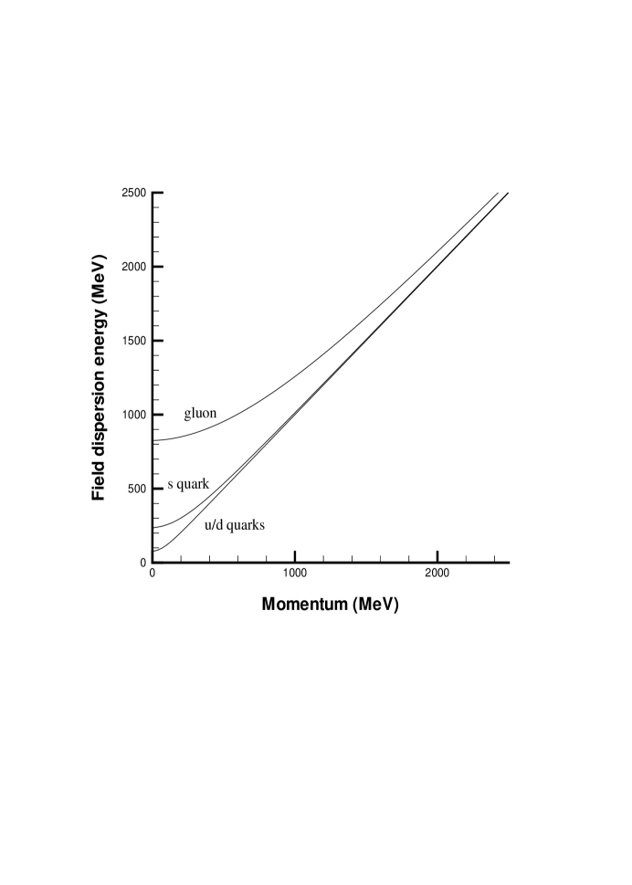
FIG. 1.: Quasiparticle energies for the $u/d,s$ quarks and the gluon [1].

FIG. 2.: Pseudoscalar and vector($L=0$) TDA and RPA meson spectra. Only the RPA provides the correct chiral limit for the pion.

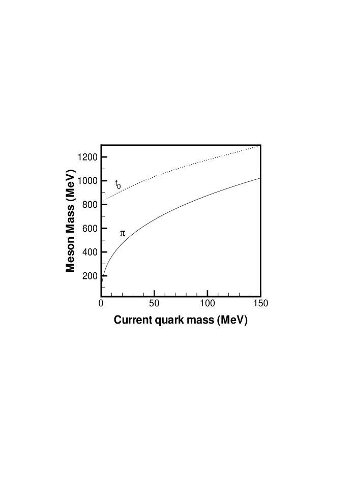
FIG. 3.: Chiral symmetry in the RPA. For $m\rightarrow 0$ the pseudoscalar (solid) but not scalar (dotted) meson mass vanishes.

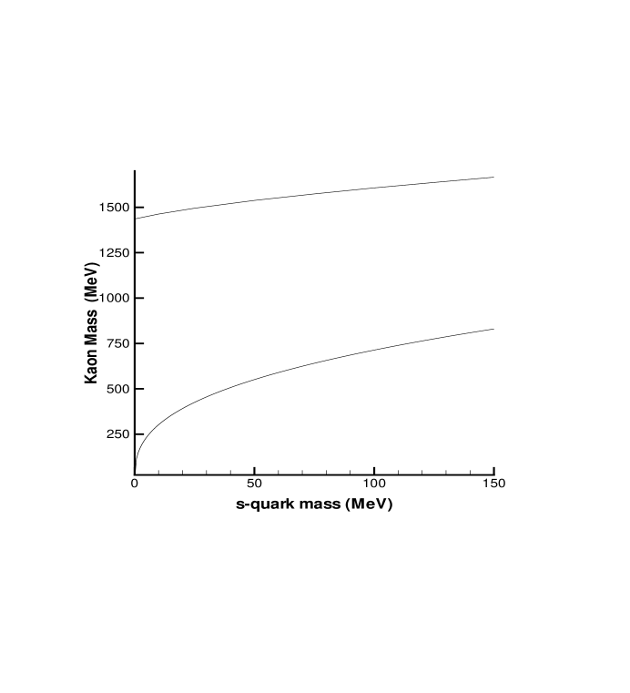
FIG. 4.: Chiral behavior of the kaon and first radial excitation. Light quark mass is 0 $MeV$.

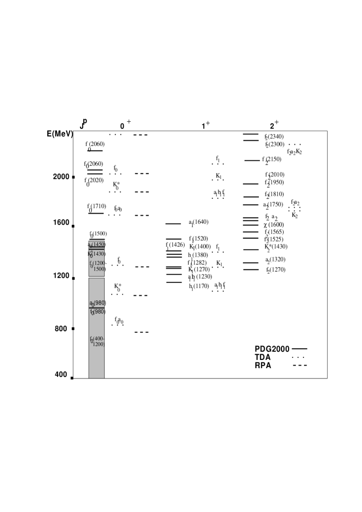
FIG. 5.: Scalar, pseudovector and tensor ($L=1$) meson spectra. Above 1 $GeV$, the TDA (dots) and RPA (dashes) are essentially identical.

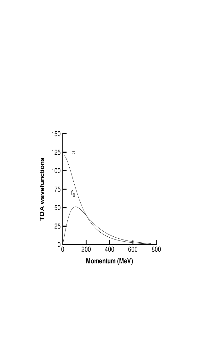
FIG. 6.: Ground state TDA wave functions for the pseudoscalar $\pi$ and scalar $f_{0}$.

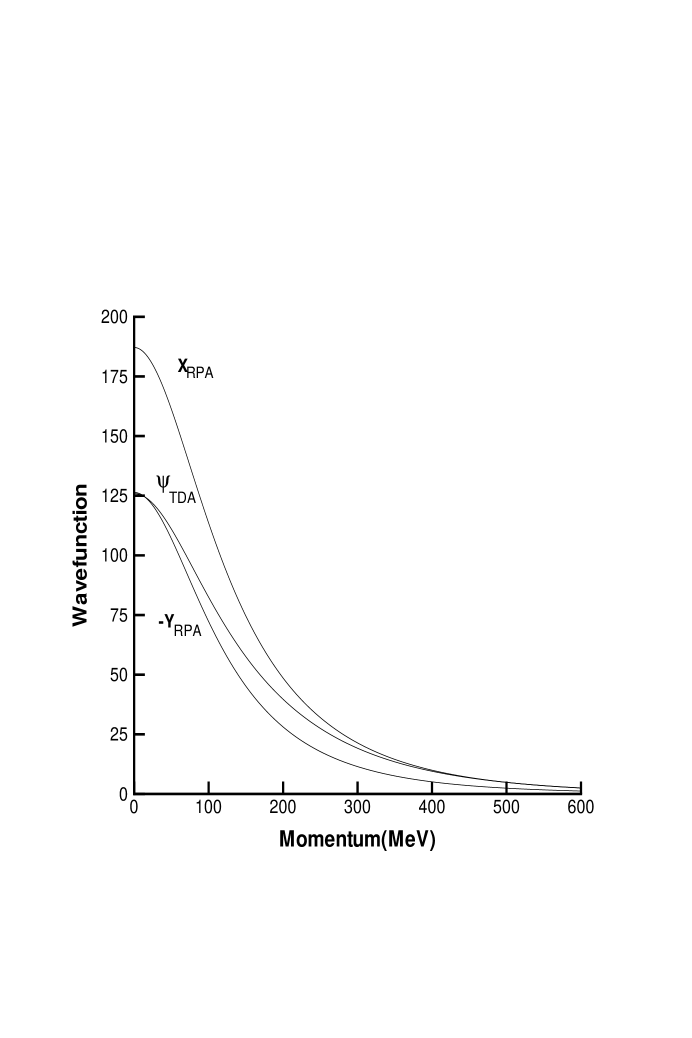
FIG. 7.: TDA and RPA ground state pion wavefunctions.

FIG. 8.: $D$ mesons ($L=0$ and $L=1$). Charmed quark mass is 1200 $MeV$, light quark is 5 $MeV$.

FIG. 9.: $D_{s}$ mesons ($L=0$ and $L=1$). Charmed (strange) quark mass is 1200 (150) $MeV$.

FIG. 10.: Charmonium system ($L=0$ and $L=1$). Charmed quark mass is 1200 $MeV$.

REFERENCES

• [1] A. P. Szczepaniak, E. S. Swanson, C.-R. Ji, and S. R. Cotanch, Phys. Rev. Lett. 76, 2011 (1996).
• [2] D. G. Robertson, E. S. Swanson, A. P. Szczepaniak, C.-R. Ji, and S. R. Cotanch, Phys. Rev. D 59, 074019 (1999).
• [3] F. J. Llanes-Estrada and S. R. Cotanch, Phys. Rev. Lett. 84, 1102 (2000).
• [4] E. Gubankova, C.-R. Ji, and S. R. Cotanch, Phys. Rev. D, 62 (2000).
• [5] A. Le Yaouanc, L. Oliver. O. Pene, and J.-C. Raynal, Phys. Rev. D 29, 1233 (1984); A. Le Yaouanc, L. Oliver, S. Ono, O. Pene, and J.-C. Raynal, Phys. Rev. D 31, 137 (1985).
• [6] S. L. Adler and A. C. Davis, Nucl. Phys. B244, 469 (1984).
• [7] P. Bicudo and J. E. Ribeiro, Phys. Rev. D 42, 5 (1990); P. Bicudo, J. E. Ribeiro, and J. Rodrigues, Phys. Rev. C 52, 4 (1995); P. Bicudo, dissertation presented to ”Instituto Superior Tecnico de Lisboa”, 1987; P. Bicudo and J. E. Ribeiro, private communication.
• [8] R. Brockmann, W. Weise, and E. Werner, Phys. Lett. 122B, 201 (1983); V. Bernard, R. Brockmann, M. Schaden, W. Weise, and E. Werner, Nucl. Phys. A412, 349 (1984); W. Weise, Internal Review of Nuclear Physics (World Scientific), Vol. 1, 57 (1984).
• [9] D. Zwanziger, Nucl. Phys. B485, 185 (1997).
• [10] N. Brambilla and A. Vairo lectures at the 1998 Hampton University Graduate Studies, held at Thomas Jefferson National Laboratory, to be published in the proceedings.
• [11] A. P. Szczepaniak and E. S. Swanson, Phys. Rev. D 55, 3987 (1997) and preprint.
• [12] E. Gubankova, C.-R. Ji, and S. R. Cotanch, to be published and private communication.
• [13] V. A. Miransky, Dynamical Symmetry Breaking in Quantum Field Theory (World Scientific, 1993).
• [14] A. Dobado, A. Gomez-Nicola, A. L. Maroto, and J. R. Pelaez, Effective Lagrangians for the Standard Model (Springer-Verlag, New York, 1997).
• [15] J. Gasser and H. Leutwyler, Ann. Phys. 158, 142 (1984).
• [16] P. Maris and C. D. Roberts, Phys. Rev. C 56, 3369 (1997).
• [17] J. M. Eisenberg and W. Greiner, Nuclear Theory, Vol. 2 Appendix A and Vol. 3, (North Holland, 1976).
• [18] P. Ring and P. Schuck, The Nuclear Many Body Problem (Springer-Verlag, New York, 1980).
• [19] R. Mattueck, A Guide to Feynman Diagrams in the Many Body Problem (Dover Publishing, 1992).
• [20] D. J. Thouless, Nucl. Phys. 22, 78 (1961).
• [21] Eur. Phys. J. C 15, 1-878 (2000).
• [22] A. De Rujula, H. Georgi, and S. L. Glashow, Phys. Rev. D 12, 147 (1975).
• [23] P. Bicudo, Phys. Rev. C 60, 035209 (1999).
• [24] F. J. Gilman and R. Kauffman, Phys. Rev. D 36, 2761 (1987).
• [25] D. Kekez, D. Klabucar, and M. D. Scadron, hep-ph/0003234.
• [26] Th. Feldmann, Int. J. Mod. Phys. A 15, 159 (2000).
• [27] N. Isgur, hep-ph/9910272.
• [28] M. E. Rose, Elementary Theory of Angular Momentum (Dover Publications, 1995).