^,, ^,2, ^,3,

Fixed-Point Hamiltonians in Quantum Mechanics

Abstract

We show how to derive fixed-point Hamiltonians in quantum mechanics from a proposed renormalization group invariance approach that relies in a subtraction procedure at a given energy scale. The scheme is valid for arbitrary interactions that originally contain point-like singularities (as the Dirac-delta and/or its derivatives). One example of diagonalization of a fixed-point Hamiltonian illustrates the procedure for an interaction that contains regular and singular parts. In another example, the fixed point Hamiltonian is derived for the case of higher order singularities in the interaction.

Recently, it has increased the interest in the application of effective theories to represent a more fundamental theory, as Quantum ChromoDynamics (QCD), which is too much complex to be solved exactly. The program followed by Wilson and collaborators [1, 2] is of particular interest in this aspect, as it allows one to parametrize the physics of the high momentum states and work with effective degrees of freedom. In ref. [1], it was suggested the idea to use an effective renormalized Hamiltonian that, in the interaction between low-momentum states, includes the coupling with high momentum states. The renormalized Hamiltonian carries the physical information contained in the quantum system in states of high momentum. (The nonperturbative renormalization of refs. [3, 4], for the light-front field theory, can also be related with the above procedure). As an example, in the nuclear physics context, the use of effective interactions containing singularities at short distances is motivated by the development of a chirally symmetric nucleon-nucleon interaction, which contains contact interactions (Dirac-delta and its higher order derivatives) [5]. Singular contact interactions have also been considered in specific treatments of scaling limits and correlations between low-energy observables of three-body systems, in atomic and nuclear physics [6]. For other examples, see ref. [7].

A general non-perturbative renormalization scheme to treat singular interactions in quantum mechanics has been proposed in ref. [8], with applications in a nuclear physics example in ref. [9] and in an effective QCD-inspired theory of mesons in ref.  [10]. It generalizes some ideas suggested in refs. [11], by performing $n$ subtractions in the free propagator of the singular scattering equation at an arbitrary energy scale. $n$ is the smallest number necessary to regularize the integral equation. The unknown short range physics related to the divergent part of the interaction, are replaced by the renormalized strengths of the interaction, that are known from the scattering amplitude at some reference energy. In this context, the renormalization scale is given by an arbitrary subtraction point. And a sensible theory of singular interactions exists if and only if the subtraction point slides without affecting the physics of the renormalized theory [12].

The subtraction point is the scale at which the quantum mechanical scattering amplitude is known [8]. A fixed-point Hamiltonian [13, 14, 15] should have the property to be stationary in the parametric space of Hamiltonians, as a function of the subtraction point [15]. This property is realized through the vanishing derivative of the renormalized Hamiltonian, in respect to the renormalization scale. This implies in the independence of the T-matrix in respect to the arbitrary subtraction scale, and in the renormalization group equations for the scattering amplitude. As shown in ref. [8], the driving term of the $n-$subtracted scattering equation changes as the subtraction point moves due to the requirement that the physics of the theory remains unchanged. The driving term satisfies a quantum mechanical Callan-Symanzik (CS) equation [16], i.e., a first order differential equation in respect to the renormalization scale. The renormalization group equation (RGE) matches the quantum mechanical theory at scales $\mu$ and $\mu+d\mu$, without changing its physical content [17].

The purpose of the present letter is to show how one should obtain the renormalized (fixed-point) Hamiltonian for a quantum mechanical system consistent with ref. [8]. The general concept of fixed-point Hamiltonians is unified to the practical and useful theory of renormalized scattering equations [8]. The response to the relevant question on the existence and formulation of the corresponding renormalized Hamiltonian of quantum mechanical systems when the original interaction contains singular terms is given. This is important from the theoretical, as well as from the practical, point of view. The method is illustrated by the diagonalization of a renormalized Hamiltonian and also by constructing the fixed-point Hamiltonian in a situation of higher singularities in the interaction.

We start by defining the renormalized (fixed-point) Hamiltonian with the corresponding effective interaction $V_{\cal R}$:

$$H_{\cal R}=H_{0}+V_{\cal R},$$ (1)

where $H_{0}$ is the free Hamiltonian. $H_{\cal R}$ and $V_{\cal R}$ are understood as ‘fixed-point’ operators, as they should not depend on the subtraction point. The corresponding T-matrix equation of the above fixed-point Hamiltonian is given by the Lippmann-Schwinger equation for the interaction $V_{\cal R}$,

$$T_{\cal R}(E)=V_{{\cal R}}+V_{{\cal R}}G^{(+)}_{0}(E)T_{\cal R}(E)\ .$$ (2)

From the expression of $V_{\cal R}$, we should be able to derive the $n-$subtracted T-matrix equation, the perturbative renormalization of the T-matrix, and the CS equation satisfied by the driving term of the subtracted form of the scattering equation. So, considering the renormalization approach given in ref. [8], the expression of the fixed-point interaction $V_{\cal R}$ is given in terms of the driving operator of the $n-$th order subtracted equation. For an arbitrary energy $E$, the driving operator is given by $V^{(n)}(-\mu^{2};E)$, where $-\mu^{2}$ is the subtraction point in the energy space, that for convenience is chosen to be negative. $n$ is the number (order) of subtractions necessary for a complete regularization of the theory. Recalling from ref. [8], the $n-$th order subtracted equation for the T-matrix and also for the driving term $V^{(n)}\equiv V^{(n)}(-\mu^{2};E)$ are, respectively,

$$T(E)=V^{(n)}(-\mu^{2};E)+V^{(n)}(-\mu^{2};E)G^{(+)}_{n}(E;-\mu^{2})T(E),$$ (3)

$${\rm and}\;\;\;\; V^{(n)}\equiv\left[1-(-\mu^{2}-E)^{n-1}V^{(n-1)}G^{n}_{0}(-\mu^{2})\right]^{-1}V^{(n-1)}+V_{sing}^{(n)}(-\mu^{2}),$$ (4)

$${\rm where}\;\; G^{(+)}_{n}(E;-\mu^{2})\equiv\left[(-\mu^{2}-E)G_{0}(-\mu^{2})\right]^{n}G^{(+)}_{0}(E).$$ (5)

$G^{(+)}_{0}(E)=(E+{\rm i}\epsilon-H_{0})^{-1}$ is the free Green’s function corresponding to forward propagation in time. The higher-order singularities of the two-body potential are introduced in the driving term of the $n-$th order subtracted T-matrix through $V_{sing}^{(n)}(-\mu^{2})$. The interaction, $V_{sing}^{(n)}(-\mu^{2})$, are determined by physical observables.

To obtain an expression for the fixed-point interaction $V_{\cal R}$, we first move the second term in the rhs of eq. (3) to the lhs; next, we add in both sides a term containing the driving term multiplied by the free Green’s function and the T-matrix:

$$\left[1+V^{(n)}\left(G^{(+)}_{0}(E)-G^{(+)}_{n}(E;-\mu^{2})\right)\right]T(E)=V^{(n)}+V^{(n)}G^{(+)}_{0}(E)T(E).$$ (6)

As in eq. (4), in order to simplify the notation, we drop the explicit dependence of $V^{(n)}$ on $\mu^{2}$ and $E$. Multiplying the above equation by the inverse of the operator that is inside the square-brackets, we can identify the fixed-point interaction $V_{\cal R}$ considering the equivalence we want to establish between eqs. (2) and (3). So, in order to have $T_{\cal R}(E)=T(E)$,

$$V_{{\cal R}}=\left[{1+V^{(n)}\left(G^{(+)}_{0}(E)-G^{(+)}_{n}(E;-\mu^{2})\right)}\right]^{-1}V^{(n)}\ .$$ (7)

By doing this, we are identifying the fixed-point Hamiltonian, eq. (1) in our renormalization scheme.

One could observe that the above fixed-point interaction is not well defined for singular interactions; nevertheless, the corresponding T-matrix is finite, as we have shown from the equivalence with the $n-$th order subtracted equation for the T-matrix, given in ref. [8]. Essentially, the renormalization subtraction procedure that was used in ref. [8] was instrumental to write the renormalized fixed-point interaction given in eq. (7). In the following, considering the above equivalence, it should be understood that our T-matrix refers to the renormalized one ($T=T_{\cal R}$), such that we drop the index $\cal R$ from it. However, there is a clear distinction between $V^{(n)}$ and $V_{\cal R}$, such that the index cannot be dropped in this case.

In a concrete numerical application, when working with the operator $V_{{\cal R}}$, we should use a momentum regulator, that could be, for example, a sharp ultraviolet momentum cutoff ($\Lambda$). By performing the limit $\Lambda\rightarrow\infty$, the results should be the same as the ones obtained through the direct use of the subtracted scattering equations. In particular, it implies that the eigenvalues of a renormalized Hamiltonian are stable in the limit $\Lambda\rightarrow\infty$, and agree with the correct results obtained from the subtracted integral equations. This fact will be illustrated.

The physical informations that apparently are lost due to the subtractions made in the intermediate free propagator are kept in $V^{(n)}$. In the case of the two-body system, it contains the renormalized coupling constants of the singular part of the interaction, given at some energy scale $-{\mu}^{2}$. We should also notice that one subtraction in the kernel of the integral equation is enough to obtain meaningful physical results from a T-matrix that contains a Dirac-delta interaction; and at least three subtractions are necessary if the singularity of the interaction corresponds to the Laplacian of the Dirac-delta function [8]. In the case of a non-singular short-range interaction ($V$) for which $V_{sing}^{(n)}=0$, we immediately identify that $V_{{\cal R}}=V$, which is not surprising since the renormalized T-matrix is the T-matrix obtained from the conventional Lippmann-Schwinger equation.

We have initially defined a nonperturbative renormalized interaction $V_{\cal R}$, although it is natural to ask about the perturbative expansion of the renormalized T-matrix in powers of $V^{(n)}$. One can easily show that, the renormalized interaction contains the necessary counterterms to include the subtractions in each perturbative order. This can be answered by performing the expansion of the renormalized interaction $V_{\cal R}$, eq. (7), in powers of $V^{(n)}$ of order $m$. Consequently, for each order $m$ one can obtain the corresponding perturbative expansion:

$$T^{(m)}(E)=V^{(n)}\sum_{k=0}^{m-1}\left[G^{(+)}_{n}(E;-\mu^{2})V^{(n)}\right]^{k}\ .$$ (8)

Thus, each intermediate state propagation up to order $m$ is subtracted at the energy scale $-\mu^{2}$. This shows that the fixed-point Hamiltonian includes the necessary counterterms in each perturbative order, which impose a subtraction of each intermediate propagation in the perturbative expansion of the scattering amplitude. As a simple remark, eq. (8) could be obtained from eq. (3), by iterating $m-1$ times and truncating at the order $m$.

The subtraction point is arbitrary in the definition of the renormalized interaction and in principle it can be moved [12]. The change in the subtraction point requires the knowledge of the driving term $V^{(n)}$ at the new energy scale. The coefficients that appear in the driving term $V^{(n)}$ come from the prescription used to define them. The renormalization group method can be used to arbitrarily change this prescription constrained by the invariance of the physics under dislocations of the subtraction point. This condition demands the renormalized potential $V_{{\cal R}}$ to be independent on the subtraction point. It gives a definite prescription to modify $V^{(n)}$ in eq. (3), without altering the predictions of the theory. So,

$$\frac{\partial V_{\cal R}}{\partial\mu^{2}}=0\;\;\;\;{\rm and}\;\;\;\;\frac{\partial H_{\cal R}}{\partial\mu^{2}}=0;$$ (9)

the renormalized Hamiltonian does not depend on $\mu$; it is a fixed-point Hamiltonian in this respect. From eqs. (2) and (9), the renormalized T-matrix also does not dependent on $\mu$,

$$\frac{\partial T(E)}{\partial\mu^{2}}=0\ .$$ (10)

The renormalization group equation, satisfied by the running driving term $V^{(n)}$ in respect to the sliding subtraction point, follows by using the null-derivative condition, given by eq. (9) in eq. (7):

$$\frac{\partial V^{(n)}}{\partial\mu^{2}}=-V^{(n)}\frac{\partial G^{(+)}_{n}(E;-{\mu}^{2})}{\partial\mu^{2}}V^{(n)}\ .$$ (11)

Thus, we reobtain the nonrelativistic Callan-Symanzik equation [8], which reflects the invariance of the subtracted scattering equation under the modification of the subtraction point. The equation (11) expresses the invariance of the renormalized T-matrix under dislocation of the subtraction point. The boundary condition is given by $V^{(n)}=V^{(n)}(-{\overline{\mu}}^{2};E)$ at the reference scale $\overline{\mu}$. The subtracted potential $V^{(n)}$ obtained by solving the differential equation (11) is equal to the T-matrix for $E=-\mu^{2}$, relating the sliding scale to the energy dependence of the T-matrix itself. In particular, for $n=1$, eq. (11) is the differential form of the renormalized equation for the T-matrix

$$\left.\frac{d}{dE}T(E)\right|_{E=-\mu^{2}}=-T(-\mu^{2})G_{0}^{2}(-\mu^{2})T(-\mu^{2}).$$ (12)

This concludes our discussion on the invariance of the fixed-point Hamiltonian under renormalization group transformation, in case of singular potentials. As we have seen, the fixed-point Hamiltonian contains the renormalized coefficients/operators that carry the physical informations of the quantum mechanical system, as well as all the necessary counterterms that make finite the scattering amplitude.

Next, we present two examples to illustrate the present approach. In the first example, the numerical diagonalization of the regularized form of the fixed-point Hamiltonian for a two-body system with a Yukawa plus a Dirac-delta interaction is performed, and the observable (eigenvalues) are shown to be independent on the energy-point $-\mu^{2}$ where the subtraction is done; the results are shown to be stable in the infinite momentum cutoff. In another example, we derive the explicit form of the renormalized potential for an example of four-term singular bare interaction.

1. Renormalized Hamiltonian diagonalization

Let us consider a two-body system with a Yukawa plus Dirac-delta interaction

$$\langle\vec{p}|V_{\cal R}|\vec{q}\rangle=\langle\vec{p}|V|\vec{q}\rangle+\frac{\lambda_{\delta}}{2\pi^{2}}=\frac{1}{2\pi^{2}}\left(\frac{-2}{|\vec{p}-\vec{q}|^{2}+\eta^{2}}+\lambda_{\delta}\right),$$ (13)

where $\lambda_{\delta}$ is the singular part of the renormalized or fixed point interaction; and $\eta$ is a constant that is given by the inverse of the range of the regular part of the interaction. The strength $\lambda_{\delta}$ can be derived from the full renormalized T-matrix given in eq. (2):

$$\left(1-VG^{(+)}_{0}(E)\right)T_{\cal R}(E)=V+|\chi\rangle\frac{\lambda_{\delta}}{2\pi^{2}}\langle\chi|\left[1+G^{(+)}_{0}(E)T_{\cal R}(E)\right]\ .$$ (14)

By defining the T-matrix of the regular potential $V$ as $T^{V}(E)=\left(1-VG^{(+)}_{0}(E)\right)^{-1}V$, and using the identity $\left(1-VG^{(+)}_{0}(E)\right)^{-1}=\left(1+T^{V}(E)G^{(+)}_{0}(E)\right)$, one can easily obtain

$$\hskip-19.91684ptT_{\cal R}(E) = T^{V}(E)+\frac{\left(1+T^{V}(E)G^{(+)}_{0}(E)\right)|\chi\rangle\langle\chi|\left(1+G^{(+)}_{0}(E)T^{V}(E)\right)}{\displaystyle\frac{2\pi^{2}}{\lambda_{\delta}}-\langle\chi|G^{(+)}_{0}(E)|\chi\rangle-\langle\chi|G^{(+)}_{0}(E)T^{V}(E)G^{(+)}_{0}(E)|\chi\rangle}\ .$$ (15)

In this case, one subtraction is enough to render finite the theory. At the subtraction point $-\mu^{2}$, the above equation defines the T-matrix of eq. (4) for $n=1$:

$$V^{(1)} = T^{V}(-\mu^{2})+\frac{\left(1+T^{V}(-\mu^{2})G_{0}(-\mu^{2})\right)|\chi\rangle\langle\chi|\left(1+G_{0}(-\mu^{2})T^{V}(-\mu^{2})\right)}{\displaystyle\frac{2\pi^{2}}{\lambda_{\delta}}-\langle\chi|G_{0}(-\mu^{2})|\chi\rangle-\langle\chi|G_{0}(-\mu^{2})T^{V}(-\mu^{2})G_{0}(-\mu^{2})|\chi\rangle}\ .$$ (16)

The denominator of the second term of eq.(16) at an arbitrary energy $-\mu^{2}$ is defined by a constant $C^{-1}(-\mu^{2})$, such that

$$2\pi^{2}C^{-1}(-\mu^{2})\equiv 2\pi^{2}\lambda_{\delta}^{-1}-\langle\chi|G_{V}(-\mu^{2})|\chi\rangle\ ,$$ (17)

where $G_{V}(-\mu^{2})=-\left(\mu^{2}+H_{0}+V\right)^{-1}=G_{0}(-\mu^{2})\left(1+T^{V}(-\mu^{2})G_{0}(-\mu^{2})\right)$. The fixed-point structure of the renormalized potential (13), $\partial V_{\cal R}/\partial\mu^{2}=0$ ($\partial\lambda_{\delta}/\partial\mu^{2}=0$), defines the functional form of $C(-\mu^{2})$ on the subtraction point:

$$2\pi^{2}C^{-1}(-\mu^{\prime 2})-2\pi^{2}C^{-1}(-\mu^{2})=\langle\chi|\left(G_{V}(-\mu^{2})-G_{V}(-\mu^{\prime 2})\right)|\chi\rangle.$$ (18)

In case that the subtraction point is chosen to be one of the binding energies of the physical system, $\mu^{2}=\mu^{2}_{B}$, $C^{-1}(-\mu_{B}^{2})=0$. So, from eq.(16), we obtain

$$\lambda_{\delta}^{-1}=\frac{2}{\pi}\int_{0}^{\Lambda}dpp^{2}\frac{-1}{\mu_{B}^{2}+p^{2}}+\frac{1}{2\pi^{2}}\int d^{3}p\frac{\Theta(\Lambda^{2}-p^{2})}{\mu_{B}^{2}+p^{2}}\int d^{3}q\frac{\Theta(\Lambda^{2}-q^{2})}{\mu_{B}^{2}+q^{2}}{\langle\vec{p}|T^{V}(-\mu_{B}^{2})|\vec{q}\rangle},$$ (19)

where the momentum cutoff $\Lambda$ was included through the step function $\Theta(x)$ (defined as $0$ for $x<0$ and $1$ for $x>0$). With the cutoff parameter $\Lambda$ assuming its exact limit (infinite), $\lambda_{\delta}$ contains the divergences in the momentum integrals that exactly cancels the infinities in eq.(2). We have to emphasize that, the role of the cutoff parameter $\Lambda$ is just of a regulator of the integrals that, at the end, should disappear in a simple limit $\infty$, without affecting the physical results. The relevant scale parameter, where the physical information is supplied, is the energy-point $-\mu^{2}_{B}$. As it will be shown, the results will not be affected by a specific choice of the position of the subtraction point.

Once $V_{R}$ is defined, as in eq.(13), we can perform the numerical diagonalization of the fixed-point Hamiltonian (1), and obtain the bound-states $\varepsilon$. The corresponding Schrödinger equation, in the $s-$wave, and in units such that $\hbar^{2}/(2m)=1$, can be written as

$$H_{\cal R}\Psi(p)=p^{2}\Psi(p)+{\frac{2}{\pi}}\int_{0}^{\Lambda}q^{2}dq\left[\frac{-1}{2pq}\ln\left(\frac{\eta^{2}+(p+q)^{2}}{\eta^{2}+(p-q)^{2}}\right)+\lambda_{\delta}\right]\Psi(q)=\varepsilon\Psi(p)\ ,$$ (20)

where $\lambda_{\delta}$, given by the renormalization prescription, keeps constant $\mu_{B}^{2}$, chosen as one of the bound-state energies. To solve numerically this example, we first choose arbitrarily a regular reference potential, with the matrix elements given by $\langle\vec{p}|V|\vec{q}\rangle=$ $-\left[\pi^{2}\left(|\vec{p}-\vec{q}|^{2}+\eta^{2}\right)\right]^{-1}$ $-\left[\pi^{2}\left(|\vec{p}-\vec{q}|^{2}+\eta^{2}_{S}\right)\right]^{-1}$, with $\eta^{2}=0.01$ and $\eta_{S}^{2}=1$ ($\eta^{2}$ and $\eta^{2}_{S}$, as well as the energies $\varepsilon$, are given in units of inverse-squared length). This reference potential produces three bound-state energies: $\varepsilon^{(0)}=-$2.3822, $\varepsilon^{(1)}=-$0.20297 and $\varepsilon^{(2)}=-$0.020643. Next, the short-range part of the reference potential is replaced by the Dirac-delta interaction. This singular interaction together with the long-range part is renormalized with the physical condition being supplied by one of the bound-state energies. This is the observable that is supposed to be known in our hypothetical example. So, the subtraction point $-\mu^{2}$ will be given by this energy. At the same time that $\mu^{2}$ is regularizing the formalism, via a subtraction procedure, it is also carrying the relevant physical information in the present Hamiltonian renormalization approach.

.

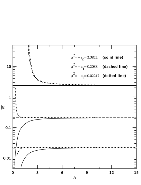
Figure 1: The bound-state energies, $\varepsilon$, of the Hamiltonian given in example 1, are shown to converge to the same exact results, in the limit $\Lambda\to\infty$ ($\Lambda=$ momentum cut-off), irrespectively to the value of the energy-scale parameter $-\mu^{2}$ that is used to renormalize the theory. One of the three bound-state energies is used to define the subtraction point $-\mu^{2}$; the other two result from the diagonalization of the renormalized Hamiltonian. $\mu$, $\Lambda$, and $\sqrt{|\varepsilon|}$ are given in units of momentum.

Our results are shown in Fig. 1 for the eigenvalues of the Hamiltonian, as functions of the momentum cutoff parameter $\Lambda$. The specific choice of the subtraction point $-\mu^{2}$ (one of the three straight lines) does not affect the final results. They are exact in the limit $\Lambda\to\infty$. Fig. 1 shows three sets of results; for each one, the value of $-\mu^{2}$ has a specific definition, given by one of the “known” energies. In solid lines, we have the results for the first and second excited states, when $\mu^{2}=$ $-\varepsilon^{(0)}=$ 2.3822. The exact results, $\varepsilon^{(1)}=-$0.2088 and $\varepsilon^{(2)}=-$0.02217, are reached when $\Lambda\to\infty$. In the same way, we obtain the results given by the other two sets, with $\mu^{2}=$ $-\varepsilon^{(1)}=$ 0.2088 (dashed-lines), and with $\mu^{2}=$ $-\varepsilon^{(2)}=$ 0.02217 (dotted-lines). As shown, in this diagonalization procedure, the results are stable when $\Lambda\to\infty$, and converge to the exact values, that can be given by the real poles of the T-matrix: $\varepsilon^{(0)}=-$2.3822, $\varepsilon^{(1)}=-$0.2088 and $\varepsilon^{(2)}=-$0.02217.

This example gives a simple and clear picture about what we have stated in Eq. (9): that the renormalized Hamiltonian does not depend on the choice of $\mu$; it is a fixed-point Hamiltonian in this respect.  The momentum cutoff $\Lambda$, used as an instrumental regulator, disappears in the present approach as a natural infinite limit of the integrals, where all the infinities presented in the formalism are canceled.

2. Renormalized Hamiltonian for a four-term singular interaction

Here we derive the explicit form of the renormalized potential for an example of four-term singular bare interaction that, after partial-wave decomposition to the $s-$wave, is given by

$$\langle p|V|q\rangle=\sum_{i,j=0}^{1}\lambda_{ij}p^{2i}q^{2j}\;\;\;(\lambda_{ij}=\lambda_{ji}^{*})\ .$$ (21)

The renormalized strengths of the interaction are known from the physical scattering amplitude at reference energy $-\overline{\mu}^{2}$

$$\langle p|T(-{\overline{\mu}}^{2})|q\rangle=\lambda_{{\cal R}00}+\lambda_{{\cal R}10}(p^{2}+q^{2})+\lambda_{{\cal R}11}p^{2}q^{2}\ ,$$ (22)

where for simplicity we suppose $\lambda_{{\cal R}10}$ real. The physics of the two-body system with the bare interaction of eq. (21) is completely defined by the values of the renormalized strengths, $\lambda_{{\cal R}ij}$, at the reference energy $-\overline{\mu}^{2}$.

In the Lippman-Schwinger equation, the potential given by eq. (21) implies in integrals that diverge at most as $p^{5}$, requiring at least three subtractions to obtain finite integrals. With $n=3$ in eq. (7), from the recurrence relationship (4), we obtain the following equations:

$$\langle p|V^{(1)}(-{\overline{\mu}}^{2})|q\rangle=\lambda_{{\cal R}00}\;,\;\;\;\;\;\langle p|V^{(2)}(-{\overline{\mu}}^{2};k^{2})|q\rangle=\left[\lambda_{{\cal R}00}^{-1}+I_{0}\right]^{-1}\;,$$ (23)

$$\langle p|V^{(3)}(-{\overline{\mu}}^{2};k^{2})|q\rangle=\overline{\lambda}_{{\cal R}00}+\lambda_{{\cal R}10}(p^{2}+q^{2})+\lambda_{{\cal R}11}p^{2}q^{2}\ ,$$

$${\rm with} \overline{\lambda}_{{\cal R}00}\equiv\left[\lambda_{{\cal R}00}^{-1}+I_{0}+I_{1}\right]^{-1}$$

$${\rm and} I_{i=0,1}\equiv I_{i}(k^{2},{\overline{\mu}}^{2})\equiv\frac{2}{\pi}\int^{\infty}_{0}dqq^{2}\frac{({\overline{\mu}}^{2}+k^{2})^{1+i}}{({\overline{\mu}}^{2}+q^{2})^{2+i}}=\frac{({\overline{\mu}}^{2}+k^{2})^{1+i}}{(2{\overline{\mu}})^{1+2i}}\ .$$ (24)

Note that the singular term, as shown in eq. (4), is introduced for $n=3$ in $V^{(3)}$ of eq. (23). Also, when $k^{2}=-\mu^{2}$ we have $I_{i}=0$ and $\overline{\lambda}_{{\cal R}00}=\lambda_{{\cal R}00}$. The renormalized interaction is obtained analytically in this example. By introducing $V^{(3)}(-\overline{\mu}^{2},k^{2})$ of eq. (23) in eq. (7),

$$\langle p|V_{{\cal R}}|q\rangle=\sum_{i,j=0}^{1}\Lambda_{ij}(k^{2})p^{2i}q^{2j}\;\;\;(\Lambda_{ij}=\Lambda_{ji})\ ,$$ (25)

where $\Lambda_{ij}$, that will not depend on the subtraction point, are given by:

$$\Lambda_{00}(k^{2}) = \frac{\overline{\lambda}_{{\cal R}00}-\left(\overline{\lambda}_{{\cal R}00}K_{1}+\lambda_{{\cal R}10}K_{2}\right)\Lambda_{10}}{1+\overline{\lambda}_{{\cal R}00}K_{0}+\lambda_{{\cal R}10}K_{1}};$$ (26)

$$\Lambda_{11}(k^{2}) = \frac{\lambda_{{\cal R}11}-\left(\lambda_{{\cal R}10}K_{0}+\lambda_{{\cal R}11}K_{1}\right)\Lambda_{10}}{1+\lambda_{{\cal R}11}K_{2}+\lambda_{{\cal R}10}K_{1}};$$ (27)

$$\Lambda_{10}(k^{2}) = \frac{\lambda_{{\cal R}10}+(\lambda_{{\cal R}10}^{2}-\overline{\lambda}_{{\cal R}00}\lambda_{{\cal R}11})K_{1}}{1+D+(\lambda_{{\cal R}10}^{2}-\overline{\lambda}_{{\cal R}00}\lambda_{{\cal R}11})(K_{1}^{2}-K_{0}K_{2})},\;\;\;$$ (28)

with $D\equiv\overline{\lambda}_{{\cal R}00}K_{0}+\lambda_{{\cal R}10}K_{1}+\lambda_{{\cal R}11}K_{2}+\lambda_{{\cal R}10}K_{1}$ and

$$K_{i=0,1,2} \equiv K_{i}(k^{2},{\overline{\mu}}^{2})\equiv\frac{2}{\pi}\int_{0}^{\infty}\frac{dqq^{2i+2}}{k^{2}-q^{2}}\left[1-\left(\frac{\overline{\mu}^{2}+k^{2}}{\overline{\mu}^{2}+q^{2}}\right)^{3}\right].$$ (29)

$K_{i}$ are the divergent integrals that exactly cancels the infinities of the Lippman-Schwinger equation obtained with the renormalized interaction, eq. (25). The integrands of these integrals are given by the kernel of eq. (7) with $n=3$.

The derivatives ${\partial\Lambda_{ij}}/{\partial\mu^{2}}$ vanish due to the arbitrariness of the subtraction point. These conditions on the derivatives are given by the explicit form of eq. (9) in the case of the four-term singular potential. The dependence of the coefficients $\lambda_{{\cal R}00}$, $\lambda_{{\cal R}10}$ and $\lambda_{{\cal R}11}$ on the sliding scale $\mu$ can be computed either from the above conditions or directly from eq. (11). The boundary condition of the RGE first order differential equation should be given for each scattering energy $k^{2}$, considered as a parameter, at the reference value of the subtraction point $-\overline{\mu}^{2}$. This concludes our example of a derivation of the renormalized Hamiltonian, with the corresponding renormalized interaction given by (25).

In summary, the fixed-point Hamiltonian emerges as a consequence of the renormalized $n$-subtracted scattering equation for the T-matrix. It does not depend on the position of the subtraction point, $-\mu^{2}$, where the physical information is supplied to the theory. As shown, it naturally includes the renormalization group invariance properties of quantum mechanics with singular interactions, as expressed by the nonrelativistic Callan-Symanzik equation. Finally, we should emphasize the wide range of applicability of renormalized Hamiltonians, from atomic and nuclear physics models to effective theories of QCD (see, for example, refs. [6]-[10]). It would be of interest a comparison between the present nonperturbative Hamiltonian renormalization approach with other given formalisms; as, for example, the approach considered in ref. [18]. However, a caution is necessary when doing such comparison, as one should note that, in the present work, the invariance of the Hamiltonian is with respect to a subtraction energy scale, in the limit of infinite momentum cutoff. The present Hamiltonian renormalization approach is particularly useful when several discrete eigenvalues are possible, since it can be diagonalized, in a regularized form, in order to obtain physical observables that are well defined in the infinite cutoff limit.

This work was partially supported by Fundação de Amparo à Pesquisa do Estado de São Paulo (FAPESP) and Conselho Nacional de Desenvolvimento Científico e Tecnológico (CNPq).

References

- [1] S.D. Glazek and K.G. Wilson, Phys. Rev. D48 (1993) 5863; Phys. Rev. D 49 (1994) 4214; Phys. Rev. D57 (1998) 3558.
- [2] M.M. Brisudová, R.J. Perry and K.G. Wilson, Phys. Rev. Lett. 78 (1997) 1227.
- [3] S. Glazek, A. Harindranath, S. Pinsky, J. Shigemitsu, and K. Wilson, Phys. Rev. D 47 (1993) 1599.
- [4] S.J. Brodsky, H.C. Pauli, and S.S. Pinsky, Phys. Rep. 301 (1998) 300.
- [5] S. Weinberg, Nucl. Phys. B363 (1991) 3; Phys. Lett. B 295 (1992) 114.
- [6] A.E.A. Amorim, L. Tomio, and T. Frederico, Phys. Rev. C46 (1992) 2224; A.E.A. Amorim, L. Tomio, and T. Frederico, Phys. Rev. C56 (1997) 2378; T. Frederico, L. Tomio, A. Delfino, and A.E.A. Amorim, Phys. Rev. A60 (1999) R9; L. Tomio, T. Frederico, A. Delfino, and A.E.A. Amorim, Few-Body Syst. Supp. 10 (1999) 203; A. Delfino, T. Frederico, M.S.Hussein and L. Tomio, Phys. Rev. C 6105 (2000) R1301; A. Delfino, T. Frederico and L. Tomio, Few-Body Syst. 28 (2000) 259.
- [7] G. P. Lepage, How to Renormalize the Schrödinger Equations, Proc. of the VIII Jorge André Swieca Summer School, pg.135, World Scientific, Singapore, 1997; nucl-th/9706029.
- [8] T. Frederico, A. Delfino and L. Tomio, Phys. Lett. B 481 (2000) 143.
- [9] T. Frederico, V.S. Timóteo, and L. Tomio, Nucl. Phys. A 653 (1999) 209.
- [10] T. Frederico and H.C. Pauli, “Renormalization of an effective light-cone QCD-inspired theory for the pion and other mesons”, hep-ph/0103233, to appear in Phys. Rev. D.
- [11] S.K. Adhikari,T. Frederico and I.D. Goldman, Phys. Rev. Lett. 74 (1995) 487; S.K.Adhikari and T.Frederico, Phys. Rev. Lett. 74 (1995) 4572.
- [12] S. Weinberg, “The Quantum Theory of Fields Vol. I, Foundations”, Cambridge University Press 1995; and “The Quantum Theory of Fields Vol. II, Modern Applications”, Cambridge University Press 1996.
- [13] K.G. Wilson, Rev. Mod. Phys.55 (1983) 583, K.G. Wilson, Phys. Rev. D2 (1970) 1438; K.G. Wilson and J. Kogut, Phys. Rep. 12 (1974) 75;
- [14] M. E. Fisher, Rev. Mod. Phys. 70 (1998) 653.
- [15] J. Zinn-Justin, “Quantum Field Theory and Critical Phenomena”, Claredon Press-Oxford 1989.
- [16] C.G. Callan, Phys. Rev. D2 (1970) 1541; K. Symanzik, Comm. Math. Phys. 16 (1970) 48; K. Symanzik, Comm. Math. Phys. 18 (1970) 227.
- [17] H. Georgi, Nucl. Phys. B 361 (1991) 339; H. Georgi, Annu. Rev. Nucl. Part. Sc. 43 (1993) 209.
- [18] M.C. Birse, J.A. McGovern, K.G. Richardson, Phys. Lett. B 464 (1999) 169; hep-ph/9808398.