Skewed parton distributions (SPDs) have been introduced as parametrizations of soft matrix elements of quark and gluon field operators between hadronic states with different momenta [1, 2, 3]. These matrix elements are relevant to hard electroproduction processes such as, for instance, deeply virtual Compton scattering (DVCS). An interesting feature of SPDs is that they are interpolating functions between ordinary parton distribution functions and hadronic form factors. More precisely, in the forward limit SPDs are given by parton distribution functions and form factors are moments of SPDs.

Because of the nonperturbative nature of the corresponding soft hadronic matrix elements information about the form of SPDs has to be taken from experiment or, alternatively, one may resort to various models [4]-[11]. In Refs. [12] and [13] an exact overlap representation of SPDs in terms of light-cone wave functions has been given.

In the present work we derive an explicit and model-independent expression for the skewed quark distribution of the pion at large momentum transfer $t$. To this end, we consider DVCS off pions. The amplitude of this process is known to factorize into a hard photon-parton scattering and a SPD [1, 2, 3]. If we additionally demand that $s,-t,-u\gg\Lambda^{2}$, where $\Lambda$ is a typical hadronic scale of the order of 1 GeV, the process is amenable to a perturbative analysis within the hard scattering approach of Ref. [14]. The amplitude then factorizes into two pion distribution amplitudes (DAs) and a hard scattering amplitude which, in lowest-order quantum chromodynamics (QCD), is given in terms of one-gluon exchange diagrams. In this way, the SPD is represented in terms of two pion DAs. We will show that our result satisfies general properties of SPDs, is continuous, and its derivatives exhibit discontinuities at the points $\pm\xi$.

The outline of the paper is the following. We start by briefly introducing our notation. We then present the derivation of the SPD of the pion at large $t$ within the hard scattering approach. Since the derivation is completely analogous to that of the two-pion distribution amplitude from the process $\gamma^{*}\gamma\to\pi\pi$ at $\Lambda^{2}\ll s\ll Q^{2}$ [15], which is related to DVCS by crossing, we will only repeat the essential steps and refer the reader to Ref. [15] for the details. We reproduce the general properties and elaborate on the behavior of our result at the points $\pm\xi$. We conclude with our summary.

Figure 1: Schematical picture of a SPD, represented by the blob.

We denote the momenta of the incoming and outgoing pions by $p$ and $p^{\prime}$, respectively (see, also, Fig. 1). In this work, we use Ji’s parametrization [16] throughout, i.e., we introduce the average momentum $\bar{p}=(p+p^{\prime})/2$, where from now on we follow the notation of Ref. [12] and employ the “bar” convention in order to define average momenta and average momentum fractions. Denoting the momentum transfer by $\Delta=p^{\prime}-p$, we can write the skewedness parameter which describes the change in plus momentum as $\xi=-\Delta^{+}/(2\bar{p}^{+})$. We define the average parton momentum $\bar{k}=(k+k^{\prime})/2$, where $k\,(k^{\prime})$ is the momentum of the emitted (absorbed) parton, and we introduce the average momentum fraction $\bar{x}=\bar{k}^{+}/\bar{p}^{+}$. With these conventions, we write the formal definition of a skewed quark distribution for a flavor $q$ in terms of a nondiagonal hadronic matrix element as [17]

$$\int\frac{dz^{-}}{2\pi}\,e^{i\bar{x}\bar{p}^{+}z^{-}}\,\langle\pi(p^{\prime})|\bar{\psi}_{q}(-z^{-}/2)\gamma^{+}\psi_{q}(z^{-}/2)|\pi(p)\rangle=2\,H_{q}(\bar{x},\xi,t),$$ (1)

where $z^{-}$ in the quark fields is a short hand for $z=[0,z^{-},{\bf 0}_{\perp}]$ in light-cone coordinates.

We now turn to a discussion of the Compton process $\gamma^{*}\pi^{+}\to\gamma\pi^{+}$ in the deeply virtual region, i.e., for $-t\ll Q^{2}$. In analogy to the nucleon case [2, 3], we can write the helicity amplitude in leading order $\alpha_{s}$ and leading twist in terms of a hard part and the SPD $H_{q}(\bar{x},\xi,t)$:

$${\cal M}_{\lambda\lambda^{\prime}} = -\frac{1}{2}\,\delta_{\lambda\lambda^{\prime}}\sum_{q}e_{0}^{2}\,e_{q}^{2}\int_{-1}^{1}d\bar{x}\,\bigg{[}\frac{1}{\bar{x}-\xi+i\,\epsilon}+\frac{1}{\bar{x}+\xi-i\,\epsilon}\bigg{]}\,H_{q}(\bar{x},\xi,t),$$ (2)

with $e_{0}$ being the positron charge and $\lambda$ and $\lambda^{\prime}$ denote the helicities of the virtual and real photon, respectively. The helicity selection rule stems from the collinear scattering of massless quarks. Note that the above expression is independent of the photon virtuality $Q^{2}$.

Demanding that $s,-t,-u\gg\Lambda^{2}$ while keeping the condition $-t\ll Q^{2}$ we can subject the process to a perturbative investigation within the hard scattering approach [14]. The helicity amplitude may then be expressed by a convolution of a hard scattering amplitude $T_{H}$ and two pion DAs $\phi_{\pi}$ [14]:

$${\cal M}_{\lambda\lambda^{\prime}}(s,t,Q^{2}) = \frac{f_{\pi}^{2}}{24}\int_{0}^{1}dx\,dy\,\phi^{*}_{\pi}(y;\mu_{F})\,T_{H}(x,y,s,t,Q^{2})\,\phi_{\pi}(x;\mu_{F}),$$ (3)

where $f_{\pi}\simeq 131$ MeV is the pion decay constant and $x,\,y$ denote the momentum fractions of the quarks relative to their respective parent hadrons. $\mu_{F}$ is the factorization scale. In leading order $\alpha_{s}/t$ only the lowest Fock state contributes to Eq. (3).

Figure 2: Representatives of the of the handbag diagrams for $\gamma^{*}\pi\to\gamma\pi$ in leading order using light-cone gauge. The remaining handbag diagrams are obtained by permutation of the photon vertices and of the fermion lines.

While the soft physics is embodied by the pion DAs, the hard scattering amplitude describes the hard photon-parton scattering. The relevant Feynman diagrams and the corresponding expressions for $T_{H}$ are related by crossing to those of the pion pair production process $\gamma^{*}\gamma\to\pi\pi$. The diagrams of that process are explicitly given in Ref. [15]. As we have discussed there it is useful to employ the gluon propagator in light-cone gauge. In this case, only particular diagrams contribute to the hard scattering amplitude in leading order, namely, those handbag diagrams where the gluon does not couple to the quark which connects the two photon vertices, see Fig. 2. The contributions of the other handbag diagrams where the gluon couples to the quark connecting the photon vertices and the contributions of the cat’s-ears diagrams where the photons couple to different quark lines are suppressed by powers of $1/Q$.

The physical picture is then such that either before or after the hard photon-quark scattering the quarks exchange a gluon. This gluon is soft relative to the dominant hard scale $Q^{2}$ and is absorbed into the SPD, i.e., the gluon is assigned to the blob in Fig. 1.

The expression for the hard scattering amplitudes can readily be obtained from those given in Ref. [15]. One simply has to replace $s\leftrightarrow t$ and, since one of the outgoing pions in the pion pair production becomes an incoming pion in the Compton process, the substitution $y\leftrightarrow 1-y$ has to be made, which exchanges the role of quark and antiquark. We have explicitly checked this crossing rule by recalculating the hard scattering amplitudes for DVCS. In order to derive the representation of $H_{q}(\bar{x},\xi,t)$ we have to calculate Eq. (3) and compare with Eq. (2). To this end, we rewrite $s$ and $u$ in terms of $\xi$ and $Q^{2}$. Up to corrections of order $t/Q^{2}$ we find:

$$s=\frac{1-\xi}{2\xi}\,Q^{2},\quad u=-\frac{1+\xi}{2\xi}\,Q^{2}.$$ (4)

Further, we express the integration variables $x$ and $y$ in terms of the average momentum fraction $\bar{x}$, defined above, and $\xi$. In the case where the photon couples to a $u$ quark, i.e., $q=u$, we have

$$y = \frac{\bar{x}-\xi}{1-\xi},\quad{\rm for\quad B1},$$ (5)

$$x = \frac{\bar{x}+\xi}{1+\xi},\quad{\rm for\quad B2}.$$ (6)

Since $0\leq x,y\leq 1$ it follows that

$$\xi\leq\bar{x}\leq 1, \quad{\rm for\quad B1},$$ (7)

$$-\xi\leq\bar{x}\leq 1, \quad{\rm for\quad B2}.$$ (8)

It is interesting to note that only diagram B2, where the gluon is exchanged after the hard photon-quark scattering, contributes to the central region $-\xi\leq\bar{x}\leq\xi$. This can be understood as follows.

The returning quark of diagram B2, i.e., the quark between the photon and gluon vertices, is off-shell and has negative momentum fraction $\bar{x}-\xi$ in the region $-\xi\leq\bar{x}\leq\xi$. Therefore, the quark may be interpreted as an antiquark with positive momentum fraction $-(\bar{x}-\xi)$ being emitted by the initial pion. But this just corresponds to the usual interpretation of a SPD in the central region: there, the SPD describes the emission of a $q\bar{q}$ pair. On the other hand, diagram B1 does not allow for such an interpretation because the gluon is exchanged before the photon-quark scattering, i.e., the emitted quark is off-shell, whereas the returning quark is on-shell and thus cannot have negative momentum fraction. Interpreting the emitted quark as an absorbed antiquark, one finds that the SPD describes the absorption of a $q\bar{q}$ pair. However, this situation is kinematically forbidden in DVCS and automatically excluded as a result of condition (7).

After the above substitutions and convoluting the leading order hard scattering amplitude with the pion DAs we obtain the helicity amplitude (3) in the limit $\Lambda^{2}\ll-t\ll Q^{2}$. For $q=u$ we have

$${\cal M}^{u}_{\lambda\lambda^{\prime}}(\xi,t)=\frac{1}{2}\,\delta_{\lambda\lambda^{\prime}}\,e_{0}^{2}e_{u}^{2}\,\frac{8\pi f_{\pi}^{2}}{9}$$

$$\times\Bigg{\{}\int_{-\xi}^{1}d\bar{x}\,\bigg{[}\frac{1}{\bar{x}-\xi+i\,\epsilon}+\frac{1}{\bar{x}+\xi-i\,\epsilon}\bigg{]}\,\frac{1+\xi}{1-\bar{x}}\,\phi_{\pi}\bigg{(}\frac{\bar{x}+\xi}{1+\xi}\bigg{)}\,\tilde{I}(\bar{x},-\xi,t;\phi^{*}_{\pi})$$

$$\hskip 10.0pt+\int_{\xi}^{1}d\bar{x}\,\bigg{[}\frac{1}{\bar{x}-\xi+i\,\epsilon}+\frac{1}{\bar{x}+\xi-i\,\epsilon}\bigg{]}\,\frac{1-\xi}{1-\bar{x}}\,\phi^{*}_{\pi}\bigg{(}\frac{\bar{x}-\xi}{1-\xi}\bigg{)}\,\tilde{I}(\bar{x},\xi,t;\phi_{\pi})\Bigg{\}},$$ (9)

where the first term results from diagram B2 and the second term from B1. The integral $\tilde{I}(\bar{x},\xi,t;\phi_{\pi})$ is defined by

$$\tilde{I}(\bar{x},\xi,t;\phi_{\pi})=\int_{0}^{1}dy\,\frac{\alpha_{s}(\mu_{R})}{t}\,\frac{(1-y)(1+\xi)+(\bar{x}+\xi)}{y(1+\xi)-(\bar{x}+\xi)}\,\frac{\phi_{\pi}(y)}{1-y}.$$ (10)

A natural choice of the renormalization scale $\mu_{R}^{2}$ is the gluon virtuality, which is typically of the order $t$. In the case of the photon coupling to the $\bar{d}$ quark, one has to make the replacements $x\rightarrow 1-x,\,y\rightarrow 1-y$ and $e_{u}^{2}\rightarrow e_{d}^{2}$ in the hard scattering amplitudes for DVCS. The calculation shows that using the isospin symmetry of the pion DA, $\phi_{\pi}(x)=\phi_{\pi}(1-x)$, the helicity amplitudes for $q=u$ and $q=\bar{d}$ are the same up to the charge factor. We find analogous counting rules for the contributions of the various helicities of the photons as in the case of the pion pair production, which is reflected by the Kronecker delta in Eq. (9). Longitudinally polarized virtual photons contribute with $1/(Q\sqrt{-t})$ and photons with opposite helicities contribute with $1/Q^{2}$.

By direct comparison of Eq. (9) with Eq. (2) we can read off the expression for the skewed $u$-quark distribution of the pion:

$$H_{u}(\bar{x},\xi,t)=-\frac{4}{9}\pi f_{\pi}^{2}\Bigg{\{} \Theta(\bar{x}+\xi)\frac{1+\xi}{1-\bar{x}}\,\phi_{\pi}\bigg{(}\frac{\bar{x}+\xi}{1+\xi}\bigg{)}\,\tilde{I}(\bar{x},-\xi,t;\phi^{*}_{\pi})$$

$$+ \Theta(\bar{x}-\xi)\frac{1-\xi}{1-\bar{x}}\,\phi^{*}_{\pi}\bigg{(}\frac{\bar{x}-\xi}{1+\xi}\bigg{)}\,\tilde{I}(\bar{x},\xi,t;\phi_{\pi})\Bigg{\}}.$$ (11)

According to our remark below Eq. (10) concerning the case $q=\bar{d}$ it is clear that $H_{\bar{d}}(\bar{x},\xi,t)=H_{u}(\bar{x},\xi,t)$. With the relation between skewed quark and antiquark distributions $H_{\bar{q}}(\bar{x},\xi,t)=-H_{q}(-\bar{x},\xi,t)$ (see, e.g., Ref. [12]), we find

$$H_{d}(\bar{x},\xi,t)=-H_{u}(-\bar{x},\xi,t).$$ (12)

for the skewed $d$-quark distribution. From the suppression of higher Fock states it immediately follows that

$$H_{s}(\bar{x},\xi,t)\equiv 0.$$ (13)

The symmetry under $\xi\leftrightarrow-\xi$ [16] is manifest in our result (11). In order to show that expression (11) complies with the polynomiality condition [4, 18] we proceed analogously as in the case of the two-pion distribution amplitude [15]. We replace the integration variable $y$ appearing in the integral $\tilde{I}(\bar{x},-\xi,t;\phi_{\pi})$ in the first term of Eq. (11) by $x$ and revert the substitutions (5) and (6). Using the binomial expansion and the relation $(a^{n}-b^{n})/(a-b)=\sum_{i=1}^{n}a^{n-i}\,b^{i-1}$ this gives

$$\int_{-1}^{1}d\bar{x}\,\bar{x}^{n-1}\,H_{u}(\bar{x},\xi,t)=-\frac{4}{9}\pi f_{\pi}^{2}\int_{0}^{1}dx\,dy\,\frac{\alpha_{s}}{t}\frac{\phi_{\pi}(x)}{1-x}\frac{\phi^{*}_{\pi}(y)}{1-y}$$

$$\times\Bigg{[}-2\sum_{\scriptstyle i=0\atop\scriptstyle{\rm even}}^{n-1}\bigg{(}\begin{array}[]{c}n-1\\ i\end{array}\bigg{)}\,x^{n-1-i}\,[(1-x)\xi]^{i}+2\xi\sum_{\scriptstyle i=1\atop\scriptstyle{\rm odd}}^{n-1}\bigg{(}\begin{array}[]{c}n-1\\ i\end{array}\bigg{)}\,x^{n-1-i}\,[(1-x)\xi]^{i}$$ (18)

$$\hskip 135.0pt-(1-\xi^{2})\sum_{i=1}^{n-1}[y+(1-y)\xi]^{n-1-i}\,[x-(1-x)\xi]^{i-1}\Bigg{]}.$$ (19)

Obviously, the right hand side is a polynomial of order $n$ in $\xi$. Using relation (12) we find for the first moment, i.e., $n=1$, the pion form factor in the collinear hard scattering approximation [14]:

$$\int_{-1}^{1}d\bar{x}\,H_{u}(\bar{x},\xi,t)=\frac{8\pi f_{\pi}^{2}}{9}\int_{0}^{1}dx\,dy\,\frac{\alpha_{s}}{t}\frac{\phi_{\pi}(x)}{1-x}\frac{\phi^{*}_{\pi}(y)}{1-y}.$$ (20)

Phenomenological investigations of the $\pi$-$\gamma$-transition form factor strongly indicate that the pion DA is close to its asymptotic form $\phi_{\rm as}(x)=6x(1-x)$ [19]. Taking this as an example the skewed $u$-quark distribution reads

$$H_{u}(\bar{x},\xi,t)=-16\pi f_{\pi}^{2}\frac{\alpha_{s}}{t}\Bigg{\{} \Theta(\bar{x}+\xi)\,\frac{\bar{x}+\xi}{1+\xi}\bigg{[}1+\frac{\bar{x}-\xi}{1-\xi}\ln\bigg{|}\frac{1-\bar{x}}{\bar{x}-\xi}\bigg{|}\bigg{]}$$

$$+ \Theta(\bar{x}-\xi)\,\frac{\bar{x}-\xi}{1-\xi}\bigg{[}1+\frac{\bar{x}+\xi}{1+\xi}\ln\bigg{|}\frac{1-\bar{x}}{\bar{x}+\xi}\bigg{|}\bigg{]}\Bigg{\}}.$$ (21)

The result is shown in Fig. 3. As we can see the skewed quark distribution is logarithmically divergent at the point $\bar{x}=1$. This divergence has the same origin as the divergence of the perturbative limit of the two-pion DA at $z=\zeta$ [15] and reflects the breakdown of the collinear hard scattering approach at the endpoints where the virtualities of the internal partons, in particular the one of the gluon, become small. For a detailed qualitative and quantitative discussion of this issue see Ref. [15].

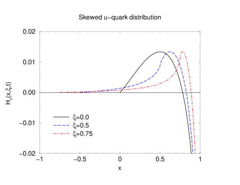
Figure 3: The SPD (21) at different values of $\xi$ and $-t=10$ GeV².

Only little is known about the behavior of SPDs at the points $\bar{x}=\pm\xi$. It has been pointed out in Ref. [3] that the continuity of SPDs at these points is necessary for the factorization in DVCS and other hard electroproduction processes. Inspection of expression (21) shows that our result is indeed continuous at $\bar{x}=\pm\xi$. Its derivatives at $\bar{x}=\pm\xi$, however, do not exist. This means that our result for the skewed quark distribution at large $t$ is an example of a SPD, the derivatives of which manifestly have singularities at these points. It can easily be seen that this is not only true in the case where we utilize the asymptotic form of the pion DA in Eq. (11). The pion DA has an expansion in terms of Gegenbauer polynomials [14] and using an arbitrary finite number of terms in this expansion one always finds singularities of the derivatives at $\bar{x}=\pm\xi$. Note that SPDs which result from integrating double distributions show the same behavior at these points [18]. For a discussion of the complete twist-2 structure of double distributions see Ref. [17].

Finally, we remark that the determination of the factorization scale of the pion DAs as well as that of the SPD requires an analysis of QCD corrections to the process amplitude. Such an analysis is, however, beyond the scope of this work.

To summarize, we have used the hard scattering approximation to perturbatively analyze DVCS off pions in the limit $\Lambda^{2}\ll-t\ll Q^{2}$, where $\Lambda$ is of ${\cal O}(1$ GeV). Within this approach, we have derived an explicit and model-independent representation of the skewed quark distribution of the pion at large momentum transfer $t$ in terms of pion DAs. Employing light-cone gauge we have found that the dominant contributions to the process come from the usual handbag diagrams, whereas contributions from gluons attached to the hard part of the diagram as well as contributions from the cat’s-ears diagrams are suppressed by powers of $1/Q$. We have shown that our result is fully consistent with the symmetry relation and the polynomiality condition and verified that the first moment of the SPD reproduces the well known expression for the pion form factor in the collinear hard scattering approximation. Furthermore, the SPD is continuous and its derivatives are discontinuous at the points $\pm\xi$.

Acknowledgements. I would like to thank M. Diehl, D. Müller, R. Jakob, P. Kroll, and B. Postler for useful discussions. Financial support by the Deutsche Forschungsgemeinschaft is acknowledged.

In expressions (10) and (14)–(16), the Mandelstam variable $t$ should be replaced with $(-t)$. In Eq. (11), the argument of the pion distribution amplitude $\phi_{\pi}^{*}$ in the second term in curly brackets should read $(\bar{x}-\xi)/(1-\xi)$ instead of $(\bar{x}-\xi)/(1+\xi)$.

A further typo is in Eq. (16), where the first term in the square brackets is to be replaced with 1/2. The correct expression thus reads

$$H_{u}(\bar{x},\xi,t)=-16\pi f_{\pi}^{2}\frac{\alpha_{s}}{(-t)}\Bigg{\{} \Theta(\bar{x}+\xi)\,\frac{\bar{x}+\xi}{1+\xi}\bigg{[}\frac{1}{2}+\frac{\bar{x}-\xi}{1-\xi}\ln\bigg{|}\frac{1-\bar{x}}{\bar{x}-\xi}\bigg{|}\bigg{]}$$

$$+ \Theta(\bar{x}-\xi)\,\frac{\bar{x}-\xi}{1-\xi}\bigg{[}\frac{1}{2}+\frac{\bar{x}+\xi}{1+\xi}\ln\bigg{|}\frac{1-\bar{x}}{\bar{x}+\xi}\bigg{|}\bigg{]}\Bigg{\}}\ .$$

Consequently, the plot of the skewed quark distribution as shown in Fig. 3 is incorrect.

The above result for $H_{u}(\bar{x},\xi,t)$ agrees with the result reported in Ref. [1], where a different convention for the pion decay constant has been used with $f_{\pi}\simeq 93$ MeV, whereas in the present work we use $f_{\pi}\simeq 131$ MeV.

Acknowledgments. I would like to thank M. Diehl and X. Ji for correspondence.

References

- [1] D. Müller, D. Robaschik, B. Geyer, F. M. Dittes, and J. , Fortschr. Phys. 42, 101 (1994), [hep-ph/9812448].
- [2] X. Ji, Phys. Rev. Lett. 78, 610 (1997), [hep-ph/9603249]; Phys. Rev. D 55, 7114 (1997), [hep-ph/9609381].
- [3] A. V. Radyushkin, Phys. Lett. B 380, 417 (1996), [hep-ph/9604317]; Phys. Rev. D 56, 5524 (1997), [hep-ph/9704207].
- [4] X. Ji, W. Melnitchouk, and X. Song, Phys. Rev. D 56, 5511 (1997), [hep-ph/9702379].
- [5] V. Yu. Petrov, P. V. Pobylitsa, M. V. Polyakov, I. Börnig, K. Goeke, and C. Weiss, Phys. Rev. D 57, 4325 (1998), [hep-ph/9710270].
- [6] I. V. Anikin, A. E. Dorokhov, A. E. Maximov, L. Tomio, and V. Vento, Phys. At. Nucl. 63, 489 (2000).
- [7] A. V. Radyushkin, Phys. Rev. D 58, 114008 (1998), [hep-ph/9803316].
- [8] A. V. Afanasev, [hep-ph/9808291].
- [9] M. Diehl, Th. Feldmann, R. Jakob, and P. Kroll, Eur. Phys. J. C 8, 409 (1999), [hep-ph/9811253].
- [10] A. P. Bakulev, R. Ruskov, K. Goeke, and N. G. Stefanis, Phys. Rev. D 62, 054018 (2000), [hep-ph/0004111].
- [11] C. Vogt, Phys. Rev. D 63, 034013 (2001), [hep-ph/0007277].
- [12] M. Diehl, Th. Feldmann, R. Jakob, and P. Kroll, Nucl. Phys. B596, 33 (2001), [hep-ph/0009255].
- [13] S. J. Brodsky, M. Diehl, and D. S. Hwang, Nucl. Phys. B596, 99 (2001), [hep-ph/0009254].
- [14] G. P. Lepage and S. J. Brodsky, Phys. Rev. Lett. 43, 545 (1979); Phys. Rev. D 22, 2157 (1980).
- [15] M. Diehl, Th. Feldmann, P. Kroll, and C. Vogt, Phys. Rev. D 61, 074029 (2000), [hep-ph/9912364].
- [16] X. Ji, J. Phys. G 24, 1181 (1998), [hep-ph/9807358].
- [17] M. V. Polyakov and C. Weiss, Phys. Rev. D 60, 114017 (1999), [hep-ph/9902451].
- [18] A. V. Radyushkin, Phys. Lett. B 449, 81 (1999), [hep-ph/9810466].
- [19] I.V. Musatov and A.V. Radyushkin, Phys. Rev. D 56, 2713 (1997), [hep-ph/9702443]; P. Kroll and M. Raulfs, Phys. Lett. B 387, 848 (1996), [hep-ph/9605264].
Erratum: Skewed quark distribution of the pion at large momentum transfer
Phys. Rev. D 64, 057501 (2001) [hep-ph/0101059]
C.Vogt

References

- [1] P. Hoodbhoy, X. d. Ji and F. Yuan, hep-ph/0309085.