P. Cea^1,2, M. Consoli³, L. Cosmai^2
1 Dipartimento di Fisica, Università di Bari, via Amendola 173, I 70126 Bari, Italy
² INFN - Sezione di Bari, via Amendola 173, I 70126 Bari, Italy
³ INFN - Sezione di Catania, Corso Italia 57, I 95129 Catania, Italy

January, 2001

Abstract

Recent lattice simulations of $(\lambda\Phi^{4})_{4}$ theories in the broken phase show that : a) the shifted field propagator is well reproduced by the simple 2-parameter form ${{Z_{\rm prop}}\over{p^{2}+M^{2}_{h}}}$ at finite momenta but strongly differs for $p\to 0$  b) the bare zero-momentum two-point function $\Gamma_{2}(0)=\left.\frac{d^{2}V_{\rm eff}}{d\varphi^{2}_{B}}\right|_{\varphi_{B}=\pm v_{B}}$ gives a value of $Z_{\varphi}\equiv{{M^{2}_{h}}\over{\Gamma_{2}(0)}}$ that increases when approaching the continuum limit. This supports theoretical expectations where $v_{B}$ is related by an infinite re-scaling to the ‘physical Higgs condensate’ $v_{R}$ defined through $\left.\frac{d^{2}V_{\rm eff}}{d\varphi^{2}_{R}}\right|_{\varphi_{R}=\pm v_{R}}=M^{2}_{h}$. New lattice data collected around the phase transition confirm this scenario. By denoting $M_{\rm SB}\equiv M_{h}={\cal O}(v_{R})$ the scale of the broken phase, our results suggest the existence of a ‘hierarchy’ of scales $\Gamma_{2}(0)\ll M^{2}_{\rm SB}\ll v^{2}_{B}$ that become infinitely far in the continuum limit. This may open unexpected possibilities to reconcile an infinitesimal slope of the effective potential with finite values of $M_{h}$ and accomodate very different mass scales in the framework of a spontaneously broken theory.

1 Introduction

Spontaneous symmetry breaking through an elementary scalar field is the basic ingredient for the origin of particle masses in the Standard Model of electroweak interactions. Traditionally, the ‘condensation’ of a scalar field, i.e. the transition from a symmetric phase where $\langle\Phi\rangle=0$ to the physical vacuum where $\langle\Phi\rangle\neq 0$, has been described as an essentially classical phenomenon in terms of a classical potential (‘B=Bare’, $\lambda>0$)

$$V_{\rm cl}(\Phi_{B})={{1}\over{2}}r_{o}\Phi^{2}_{B}+{{\lambda}\over{4!}}\Phi^{4}_{B}$$ (1)

with non-trivial absolute minima for a constant value $\Phi_{B}=\pm v_{B}\neq 0$. In this picture, by expanding around the absolute minima of the classical potential say $\Phi_{B}(x)=v_{B}+h(x)$, one predicts a simple relation

$$M^{2}_{h}=V^{\prime\prime}_{\rm cl}(\Phi_{B}=v_{B})$$ (2)

between the ‘Higgs mass’ $M_{h}$ and the quadratic shape of the potential at the minima.

In the quantum theory, and on the basis of perturbation theory, Eq.(2) is believed to represent a good approximation by simply replacing the classical potential with the quantum effective potential $V_{\rm eff}$. However, beyond perturbation theory, there is an alternative description of spontaneous symmetry breaking [1, 2, 3, 4] where $M^{2}_{h}$ and the curvature of the effective potential at the non-trivial minima are different physical quantities related by an infinite renormalization in the continuum limit of quantum field theory, with potentially important consequences for particle physics and cosmology. The above result has been obtained from gaussian and post-gaussian[5] approximations to the effective potential. In view of the relevance of the issue and for the convenience of the reader, we shall briefly recapitulate the main result in the simplest case of the gaussian approximation to the energy density ${\cal E}_{G}[\varphi_{B},\Omega]$ [6, 7, 8, 9, 10]. This is obtained from the expectation value of the hamiltonian in the class of trial states with a constant $\langle\Phi_{B}\rangle=\varphi_{B}$ and shifted-field euclidean propagator

$$G(p)={{1}\over{p^{2}+\Omega^{2}}}$$ (3)

with a variational mass parameter $\Omega$. By minimization one gets the coupled equations

$$\Omega^{2}=r_{o}+{{\lambda\varphi^{2}_{B}}\over{2}}+{{\lambda}\over{2}}I_{o}(\Omega)$$ (4)

and

$$0=r_{o}\varphi_{B}+{{\lambda\varphi^{3}_{B}}\over{6}}+{{\lambda\varphi_{B}}\over{2}}I_{o}(\Omega)$$ (5)

with

$$I_{o}(\Omega)=\int{{d^{4}p}\over{(2\pi)^{4}}}{{1}\over{p^{2}+\Omega^{2}}}$$ (6)

By using Eq.(4), one can define a $\varphi_{B}-$dependent mass $\Omega=\Omega(\varphi_{B})$ and the gaussian approximation to the effective potential $V_{G}(\varphi_{B})={\cal E}_{G}[\varphi_{B},\Omega(\varphi_{B})]$ whose first derivative has the simple form [1]

$$\frac{dV_{G}}{d\varphi_{B}}=\varphi_{B}[\Omega^{2}(\varphi_{B})-{{\lambda\varphi^{2}_{B}}\over{3}}]$$ (7)

In this way, spontaneous symmetry breaking is associated with those absolute minima $\varphi_{B}=\pm v_{B}\neq 0$ where

$$\Omega^{2}(v_{B})={{\lambda v^{2}_{B}}\over{3}}\equiv M^{2}_{h}$$ (8)

Now, the zero-momentum two-point function (the inverse susceptibility) defines the quadratic shape of the potential at the non-trivial minima

$$\chi^{-1}=\Gamma_{2}(p=0)=\left.\frac{d^{2}V_{\rm eff}}{d\varphi^{2}_{B}}\right|_{\varphi_{B}=\pm v_{B}}\equiv{{M^{2}_{h}}\over{Z_{\varphi}}}$$ (9)

where we have introduced a re-scaling factor $Z=Z_{\varphi}$ defined through Eq.(9) [11]. In the gaussian approximation, by using the identities [8]

$$I_{o}(0)-I_{o}(\Omega)={{\Omega^{2}}\over{2}}[I_{-1}(\Omega)+{{1}\over{8\pi^{2}}}]$$ (10)

and the definition

$${{dI_{o}}\over{d\Omega}}\equiv-\Omega I_{-1}(\Omega)$$ (11)

we obtain

$$\frac{d^{2}V_{G}}{d\varphi^{2}_{B}}=\Omega^{2}(\varphi_{B})-{{\lambda\varphi^{2}_{B}}\over{4}}~{}{{\lambda I_{-1}(\Omega)}\over{1+{{\lambda I_{-1}(\Omega)}\over{4}}}}$$ (12)

In the symmetric vacuum where $\varphi_{B}=0$, one finds

$$\left.\frac{d^{2}V_{G}}{d\varphi^{2}_{B}}\right|_{\varphi_{B}=0}=\Omega^{2}(0)$$ (13)

while, in the broken-symmetry phase, the alternative expression

$$\left.\frac{d^{2}V_{G}}{d\varphi^{2}_{B}}\right|_{\varphi_{B}=\pm v_{B}}=M^{2}_{h}~{}{{1-{{\lambda}\over{2}}I_{-1}(M_{h})}\over{1+{{\lambda}\over{4}}I_{-1}(M_{h})}}$$ (14)

For an evaluation of Eq.(14), it is convenient to re-define the bare mass term as

$$r_{o}=-{{\lambda}\over{2}}I_{o}(0)+\Delta$$ (15)

so that the gap-equation at the absolute minima reduces to

$$0=\Delta+{{M^{2}_{h}}\over{2}}-{{\lambda M^{2}_{h}}\over{4}}[I_{-1}(M_{h})+{{1}\over{8\pi^{2}}}]$$ (16)

( $\Delta=0$ corresponds to the ‘Coleman-Weinberg regime ’ [12] where $\Omega(0)=0$). By defining

$$I_{-1}(M_{h})\equiv{{1}\over{8\pi^{2}}}\ln{{\Lambda^{2}}\over{M^{2}_{h}}}$$ (17)

and $\mu^{2}\equiv\Lambda^{2}e^{-{{16\pi^{2}}\over{\lambda}}}$,  $\Delta\equiv{{\lambda\mu^{2}}\over{32\pi^{2}}}y$,  $M^{2}_{h}\equiv\omega^{2}\mu^{2}$,  Eq.(16) becomes

$$\omega^{2}\ln{{e}\over{\omega^{2}}}=y$$ (18)

Finally, by replacing into Eq.(14), we obtain the gaussian approximation prediction for $Z_{\varphi}$ in the broken phase

$${{1}\over{Z_{\varphi}}}={{\Gamma_{2}(p=0)}\over{M^{2}_{h}}}={{{{\lambda}\over{16\pi^{2}}}\ln\omega^{2}}\over{{{3}\over{2}}-{{\lambda}\over{32\pi^{2}}}\ln\omega^{2}}}$$ (19)

that (in the range $e^{{{48\pi^{2}}\over{\lambda}}}>\omega^{2}>1$) amounts to

$$Z_{\varphi}={{24\pi^{2}}\over{\lambda\ln\omega^{2}}}-{{1}\over{2}}$$ (20)

Eq.(20) can be considered from two qualitatively different points of view. On one hand, for given values of the dimensionless parameters $y$ and $\omega^{2}$, it implies a behaviour $Z_{\varphi}\sim{{1}\over{\lambda}}$. Thus, in a continuum limit where $\Lambda\to\infty$ and $\mu^{2}$ (and hence $M^{2}_{h}=\mu^{2}\omega^{2}$) is kept fixed, one gets $Z_{\varphi}\sim\ln{{\Lambda^{2}}\over{M^{2}_{h}}}\to\infty$ implying that the ‘Higgs mass’ $M_{h}$ and the curvature of the effective potential are different physical quantities. Indeed, they would be related by an infinite renormalization in the continuum limit of quantum field theory.

On the other hand, for any given $\lambda$, i.e. when $\mu^{2}$ and $\Lambda$ are kept in a fixed ratio, Eq.(20) predicts that $Z_{\varphi}$ should also become larger while decreasing $\omega^{2}$. This corresponds to increase $y$ from negative values trying to approach the minimum value $\omega^{2}=1$. However, in this latter case, $Z_{\varphi}$ will not diverge. In fact, before reaching the value $\omega^{2}=1$, the gaussian effective potential exhibits a (weakly) first-order phase transition to the symmetric phase [1].

We stress that the gaussian-approximation prediction of a non trivial $Z_{\varphi}$ has been tested with precise lattice simulations [13, 14] performed in the Ising limit of the theory. The data show that by approaching the critical value of the hopping parameter $\kappa_{c}\sim 0.0748$ [15] from the broken phase, the quantity $Z_{\varphi}\equiv M^{2}_{h}\chi$ rapidly increases above unity. Thus, in the broken phase, $Z_{\varphi}$ is different from the more conventional quantity $Z=Z_{\rm prop}$ associated with the two-parameter form for the shifted-field propagator

$$G_{\rm pole}(p)=\frac{Z_{\rm prop}}{p^{2}+M^{2}_{h}},$$ (21)

According to ‘triviality’ [16], this latter quantity should exhibit a continuum limit $Z_{\rm prop}\to 1$ for consistency with the Källen-Lehmann decomposition. The point is that, in the broken phase, the data deviate from Eq.(21) when $p\to 0$ presaging an even more dramatic difference at $p=0$. Furthermore, the discrepancy between $Z_{\varphi}$ and $Z_{\rm prop}$ becomes larger in the limit $\kappa\to\kappa_{c}$. Therefore, it cannot be explained by introducing residual perturbative corrections that, according to ‘triviality’[16], should become smaller and smaller in the same limit. On the other hand, in the symmetric phase where Eq.(21) describes the lattice data down to $p=0$ [14], one gets $Z_{\varphi}=Z_{\rm prop}\sim 1$ as expected on the basis of Eq.(13).

After this general Introduction, we shall report in this Letter further numerical evidence for the validity of this theoretical framework by studying the $\omega-$dependence of Eq.(20). Strictly speaking, to this end, one should work at fixed $\lambda$ by changing the bare mass in the full two-parameter $\lambda\Phi^{4}$ theory, the Ising limit being just a one-parameter model. However, even in the Ising limit we can reproduce the situation of a two-parameter theory if we perform a finite-temperature simulation. Namely, by changing the value of $\kappa$ in the broken phase, we know from refs.[13, 14] that the zero-temperature value of $Z_{\varphi}$ increases when $\kappa\to\kappa_{c}$. However, for any fixed value $\kappa>\kappa_{c}$, by increasing the temperature, we shall approach the phase transition. In this case, we expect the lattice data to exhibit a qualitatively different increase of $Z_{\varphi}$, analogously to the effect induced in Eq.(20) by approaching the phase transition at fixed $\lambda$ in the full two-parameter theory.

2 Finite-temperature lattice simulation

The transition to finite-temperature field theory is easily performed by following the formalism introduced in refs.[17]. In the case of bosonic fields the partition function is

$${\cal Z}(\beta)=\int{\cal D}\Phi~{}e^{-\int^{\beta}_{0}d\tau\int d^{3}{\bf{x}}{\cal L}_{E}}$$ (22)

where $\beta=1/T$ is the inverse temperature, ${\cal{L}}_{E}$ is the Euclidean lagrangian density and the functional integral is performed over all periodic field configurations with $\Phi({\bf{x}},\tau=0)=\Phi({\bf{x}},\tau=\beta)$. In Fourier space, the compactification of the time direction leads to a discrete energy spectrum with energies $\omega_{n}={{2n\pi}\over{\beta}}$ and, therefore, to the form of a free propagator

$$G^{(\beta)}_{\rm free}(n,{\bf{p}})={{1}\over{\hat{{\bf{p}}}^{2}+\hat{p_{4}}^{2}+M^{2}}}$$ (23)

As it is well known [18], a Monte-Carlo simulation with periodic boundary conditions on an asymmetric $L^{3}_{s}~{}{\rm x}~{}L_{t}$ lattice is equivalent to a finite-temperature calculation at $\beta=L_{t}=1/T$. To this end, a one-component $(\lambda\Phi^{4})_{4}$ theory

$$S=\sum_{x}\left[\frac{1}{2}\sum_{\mu}(\Phi(x+\hat{e}_{\mu})-\Phi(x))^{2}+\frac{r_{0}}{2}\Phi^{2}(x)+\frac{\lambda_{0}}{4}\Phi^{4}(x)\right]$$ (24)

is conveniently studied in the Ising limit

$$S_{\rm Ising}=-\kappa\sum_{x}\sum_{\mu}\left[\phi(x+\hat{e}_{\mu})\phi(x)+\phi(x-\hat{e}_{\mu})\phi(x)\right]$$ (25)

with $\Phi(x)=\sqrt{2\kappa}\phi(x)$ and where $\phi(x)$ takes only the values $+1$ or $-1$.

To perform Monte-Carlo simulations of this Ising action, we have used the Swendsen-Wang [19] cluster algorithm. Statistical errors can be estimated through a direct evaluation of the integrated autocorrelation time [20], or by using the “blocking” [21] or the “grouped jackknife” [22] algorithms. We have checked that applying these three different methods we get consistent results. Lattice observables include:

(i) the bare magnetization, $v_{B}=\langle|\Phi|\rangle$, where $\Phi\equiv\sum_{x}\Phi(x)/L^{4}$ is the average field for each lattice configuration. The broken phase is found for $\kappa>\kappa_{c}$ where $\kappa_{c}\simeq 0.0748$ [15] in an infinite volume. For any $\kappa>\kappa_{c}$, we expect to detect a phase transition to the symmetric phase at some sufficiently small value of $L_{t}$.

(ii) the zero-momentum susceptibility

$$\chi=L^{4}\left[\left\langle|\Phi|^{2}\right\rangle-\left\langle|\Phi|\right\rangle^{2}\right],$$ (26)

(iii) the shifted-field propagator

$$G(p)=\left\langle\sum_{x}\exp(ipx)(\Phi(x)-v_{B})(\Phi(0)-v_{B})\right\rangle\,,$$ (27)

where $p\equiv(p_{4},{\bf{p}})$ with ${\bf{p}}=\frac{2\pi}{L_{s}}{\bf{n}}$ and $p_{4}=\frac{2\pi}{L_{t}}{n_{4}}$ where $(n_{1},n_{2},n_{3},n_{4})$ are integer-valued components, not all zero.

To extract the ‘Higgs mass’ $M_{h}$ one has to preliminarly compare the lattice data for $G(p)$ with the 2-parameter formula

$$G^{(\beta)}_{\rm fit}(n,{\bf{p}})={{Z_{\rm prop}}\over{\hat{{\bf{p}}}^{2}+\hat{p_{4}}^{2}+m^{2}_{\rm latt}}}$$ (28)

where $m_{\rm latt}$ is the mass in lattice units and $\hat{p}_{\mu}=2\sin{{p_{\mu}}\over{2}}$.

Obviously, by setting $L_{t}=L_{s}$ we re-obtain the zero temperature case studied in refs.[13, 14]. We now repeat the basic point of [14]. To realize how good the fit with Eq.(28) can be, we start at $T=0$ in the symmetric phase at $\kappa=0.0740$ on a $20^{4}$ lattice. In Fig.1, we report the same data of ref.[14] where the scalar propagator has been suitably re-scaled to show the very good quality of the fit to Eq. (28). The value of $Z_{\rm prop}$ is indicated by the dashed line while $Z_{\varphi}$ is reported in Fig.1 as a black point at $\hat{p}=0$. Notice the perfect agreement between $Z_{\varphi}$ and $Z_{\rm prop}$.

We now select a value $\kappa=0.07512$, in the broken phase, where the 2-parameter fit to the propagator data yields a comparable value for $m_{\rm latt}$ by using a $32^{4}$ lattice. However, unlike Fig. 1, the fit to Eq. (28), though excellent at higher momenta, does not reproduce the lattice data down to zero-momentum. Therefore, in the broken phase, a meaningful determination of $Z_{\rm prop}$ and $m_{\rm latt}$ requires excluding the lowest momentum points from the fit. The lattice data are shown in Fig.2.

By fixing $\kappa=0.07512$, we have now performed computations on asymmetric $L^{3}_{s}\times L_{t}$ lattices to simulate a finite-temperature system. Notice that well past the phase transition, i.e. for very small $L_{t}$, consistency requires a $p\to 0$ limit of the propagator such that $Z_{\varphi}$ and $Z_{\rm prop}$ agree to good accuracy. In fact, if running on smaller lattices one is able to re-obtain the same conditions of the symmetric-phase calculation in Fig.1, we can exclude the presence of finite-size artifacts in the zero-temperature simulation and interpret the discrepancy between $Z_{\varphi}$ and $Z_{\rm prop}$ as a real physical effect due to the presence of the scalar condensate. At the same time, the phase transition associated with spontaneous symmetry breaking can be understood as a real condensation process where the $Z_{\varphi}-Z_{\rm prop}$ discrepancy represents a distinctive non-perturbative feature.

This expectation can be checked in Fig. 3 by comparing the data taken on the $32^{3}\times 2$ lattice with those taken on the $32$-times bigger $64^{3}\times 8$ lattice when the system, however, is still in the broken phase and a meaningful determination of $m_{\rm latt}$ through Eq.(28) requires excluding the lowest momentum points from the fit.

The data for the physical observables from different lattice sizes are reported in Table 1. For all lattice sizes there is a clear evidence for a phase transition in the region $6<L_{t}<8$ where the system crosses from the broken into the symmetric phase (see Fig. 4).

We stress that the conventional interpretation of ‘triviality’, assuming $Z_{\varphi}=Z_{\mathrm{prop}}\simeq 1$, predicts that approaching the phase transition one finds $m^{2}\to 0$ and $\chi\to\infty$ in such a way that $m^{2}\chi$ remains constant. However, our data for the quantity $Z_{\varphi}\equiv m^{2}_{\rm latt}\chi$, reported in Fig. 5, exhibit a clear increase in the critical region while the corresponding value for $Z_{\mathrm{prop}}$ remains remarkably constant (see Table 1). This confirms once more that $Z_{\varphi}$, as defined in Eq.(9), and $Z_{\text{prop}}$, as defined in Eq.(21), are different physical quantities.

3 Summary and outlook

The finite-temperature simulations presented in this paper confirm the results of refs.[13, 14]. Both provide strong numerical evidence that, close to the continuum limit of quantum field theory, a naive perturbative description of a spontaneously broken $(\lambda\Phi^{4})_{4}$ is missing very important effects. Although the theory is ‘trivial’ there are non-perturbative collective effects at (and near) zero momentum producing the observed large deviations from the standard free-field-like form of the propagator Eq.(28). These deviations are responsible for the non-trivial re-scaling factor $Z_{\varphi}=M^{2}_{h}\chi$ that increases rapidly when $\kappa\to\kappa_{c}$ in the zero-temperature case and when approaching the phase transition in the finite-temperature simulations. This provides additional numerical evidence for the validity of Eq.(20) that represents a distinctive prediction and can be used, for instance, to reconcile a finite value of $M_{h}$ with an infinitesimal quadratic shape of the effective potential at its minima. Indeed, with a divergent $Z_{\varphi}$, the usual definition of the physical vacuum field $v_{R}$

$$\left.\frac{d^{2}V_{\rm eff}}{d\varphi^{2}_{R}}\right|_{\varphi_{R}=\pm v_{R}}=M^{2}_{h}$$ (29)

is related by a non-trivial infinite re-scaling to the bare ‘Higgs condensate’ $v_{B}$ in Eq.(14). Therefore, although $v_{B}$ diverges in units of $M_{h}$, one can obtain a continuum limit where both $M_{h}$ and $v_{R}$ are finite quantities setting the scale of the spontaneously broken phase $M_{\rm SB}\equiv M_{h}={\cal O}(v_{R})$. In this sense, a divergent $Z_{\varphi}$ means that spontaneous symmetry breaking introduces a mass ‘hierarchy’ [4] where $\Gamma_{2}(p=0)\ll M^{2}_{\rm SB}\ll v^{2}_{B}$ are infinitely far scales in the continuum limit since

$$Z_{\varphi}={{M^{2}_{h}}\over{\Gamma_{2}(p=0)}}={{v^{2}_{B}}\over{v^{2}_{R}}}\sim\ln{{\Lambda}\over{M_{h}}}\to\infty$$ (30)

Another interesting point concerns the actual form of the energy spectrum for the long-wavelength excitations of the broken phase. In fact, the observed differences of the propagator from Eq.(21) for $p\to 0$ imply that the energy spectrum of the broken phase $\tilde{E}({\bf{p}})$ sizeably differs from $\sqrt{{\bf{p}}^{2}+M^{2}_{h}}$ when ${\bf{p}}\to 0$. In this respect, the results of ref.[14] show that the spectrum $\tilde{E}({\bf{p}})$ approaches the form $\sqrt{{\bf{p}}^{2}+M^{2}_{h}}$ only at large ${\bf{p}}^{2}$. Also, $\tilde{E}(0)<M_{h}$ and their difference increases in the continuum limit. Such a difference, detected by studying the time-slices of the connected correlator at various values of ${\bf{p}}$, has no counterpart in the symmetric phase. In this latter case, the form $E({\bf{p}})=\sqrt{{\bf{p}}^{2}+m^{2}}$ is found [14] to reproduce the lattice data to high accuracy for all ${\bf{p}}$ down to ${\bf{p}}=0$ so that, in this case, one gets $E(0)=m$. A particularly important question concerns the stability of the results for the energy-gap $\tilde{E}(0)$ in the broken phase and for the ‘Higgs mass’ $M_{h}$ controlling the higher-momentum behaviour of the propagator. The results of [14] for $\kappa=0.076$, the case studied by Jansen et al. [24] on a $20^{4}$ lattice, show that the value of $M_{h}$, extracted from the set of higher-momentum data where one gets a good fit with Eq.(21), is remarkably stable for variations of the lattice size from $20^{4}$ to $32^{4}$. New preliminary data [25] show that the energy spectrum $\tilde{E}({\bf{p}})$ remains also stable, at least for not too small values of ${\bf{p}}^{2}$. On the other hand, by increasing the lattice size up to $32^{4}$, our present data suggest a decrease of $\tilde{E}(0)$ that, therefore, differently from $M_{h}$, may represent an infrared-sensitive quantity. A complete discussion of this point requires, however, more statistics and will be presented in a forthcoming paper [25] .

lattice	#configs.	$1/L_{t}$	$<|\Phi|>$	$m_{\mathrm{latt}}$	$\chi$	$Z_{\varphi}$	$Z_{\mathrm{prop}}$
$32^{3}\times 2$	700K	0.5	0.015980(42)	0.494362(917)	26.25(0.14)	0.963675(6389)	0.960179(1167)
$32^{3}\times 3$	835K	0.333333	0.024602(47)	0.261363(681)	93.28(0.34)	0.957328(6074)	0.955672(898)
$32^{3}\times 4$	650K	0.25	0.035326(81))	0.180635(6834)	253.60(1.09)	1.243208(94220)	0.959723(1649)
$32^{3}\times 5$	875K	0.2	0.050104(105)	0.139061(5478)	614.61(2.36)	1.785661(140851)	0.959713(1306)
$32^{3}\times 6$	725K	0.166667	0.071158(285)	0.125006(6219)	1376.14(9.58)	3.230797(322248)	0.959374(1373)
$32^{3}\times 8$	725K	0.125	0.117674(375)	0.171012(7257)	530.55(3.85)	2.331141(198569)	0.959329(1677)
$32^{3}\times 32$	400K	0	0.161778(130)	0.20623(409)	193.1(1.7)	1.233876(501)	0.9551(21)
$48^{3}\times 3$	700K	0.333333	0.013413(27)	0.261399(594)	93.65(0.35)	0.961384(5645)	0.955420(834)
$48^{3}\times 4$	460K	0.25	0.019187(47)	0.165589(2391)	255.35(1.19)	1.051909(30770)	0.956229(1257)
$48^{3}\times 5$	635K	0.2	0.027706(72)	0.118999(2923)	655.07(3.26)	1.393679(68817)	0.958973(1088)
$48^{3}\times 6$	400K	0.166667	0.044522(193)	0.114195(6459)	1919.71(15.16)	3.761108(426501)	0.960837(1577)
$48^{3}\times 8$	170K	0.125	0.116546(516)	0.157074(7182)	826.14(20.94)	3.062311(290602)	0.958064(2392)
$48^{3}\times 9$	185K	0.111111	0.136291(415)	0.180302(6762)	464.83(11.35)	2.270273(179082)	0.955628(2456)
$64^{3}\times 2$	390K	0.5	0.005626(18)	0.494478(1463)	26.14(0.17)	0.9604047(8320)	0.959913(3017)
$64^{3}\times 3$	250K	0.333333	0.008712(31)	0.260004(681)	93.52(0.74)	0.9498651(9044)	0.952527(1263)
$64^{3}\times 4$	480K	0.25	0.012439(33)	0.163052(2724)	259.16(4.95)	1.035163(39846)	0.954254(1341)
$64^{3}\times 5$	200K	0.2	0.017980(89)	0.110235(4120)	676.43(19.80)	1.234948(99135)	0.955591(1730)
$64^{3}\times 6$	90K	0.166667	0.029673(263)	0.090056(9592)	2105.82(24.60)	2.565853(547407)	0.957225(2888)
$64^{3}\times 8$	240K	0.125	0.118429(299)	0.162401(7698)	803.64(17.45)	3.184376(309700)	0.957547(2466)
$64^{3}\times 9$	245K	0.111111	0.136991(178)	0.177897(4993)	417.49(7.65)	1.985071(117215)	0.955239(2092)
$64^{3}\times 10$	150K	0.1	0.1462464(180)	0.180102(4437)	311.83(4.56)	1.519625(78097)	0.952393(2373)
$64^{3}\times 14$	80K	0.0714286	0.158104(137)	0.193444(5602)	221.91(3.73)	1.247618(75245)	0.948202(3055)
Table 1: Summary of the simulation runs for the 4d $\lambda\varphi^{4}$ model at finite temperature (Ising limit, $\kappa=0.07512$).

FIGURE 1

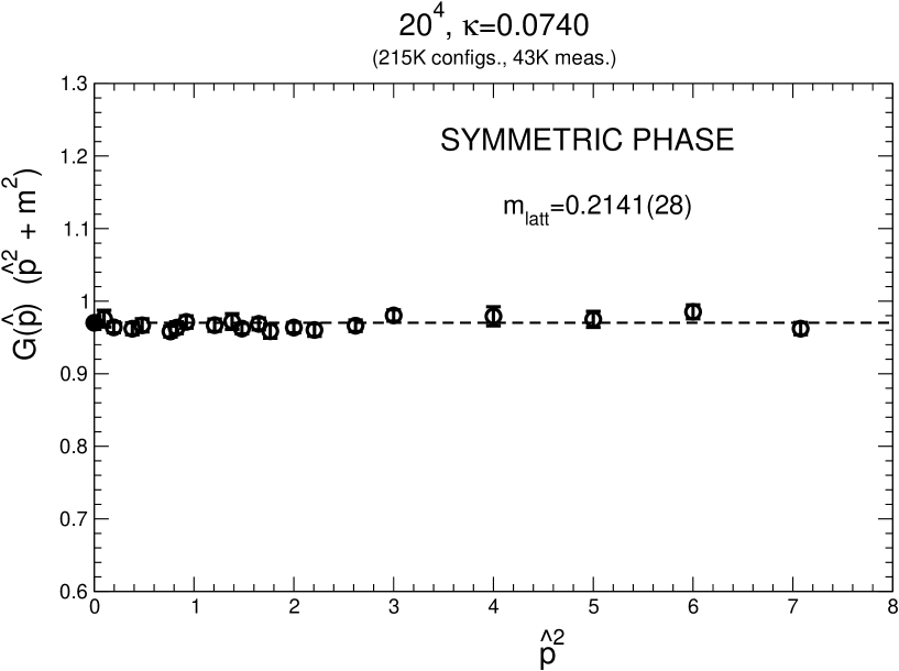
Figure 1: The lattice data for the re-scaled propagator at $\kappa=0.0740$ in the symmetric phase. The zero-momentum full point is defined as $Z_{\varphi}=m^{2}_{\mathrm{latt}}\chi$. The dashed line indicates the value of $Z_{\mathrm{prop}}$.

FIGURE 2

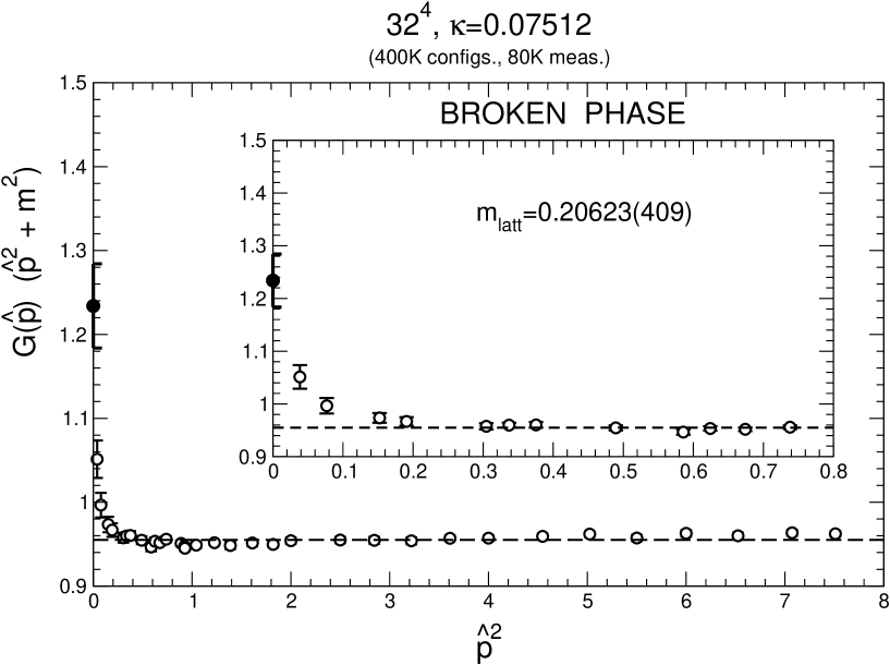
Figure 2: The lattice data for the re-scaled propagator at $\kappa=0.07512$. The zero-momentum full point is defined as $Z_{\varphi}=m^{2}_{\mathrm{latt}}\chi$. The very low momentum region is shown in the inset. The dashed line indicates the value of $Z_{\mathrm{prop}}$.

FIGURE 3

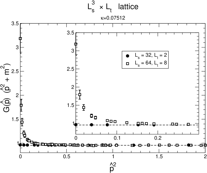
Figure 3: The same as in Fig. 2 for $L_{s}=32$ and $L_{t}=2$, and $L_{s}=64$ and $L_{t}=8$. The two sets of data are normalized in terms of the corresponding lattice masses shown in Table 1. The dashed lines indicate the same zero-temperature value $Z_{\mathrm{prop}}=0.9551$ as in Fig.2

FIGURE 4

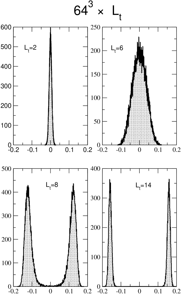
Figure 4: The distribution of the average field value for 4 values of $L_{t}$.

FIGURE 5

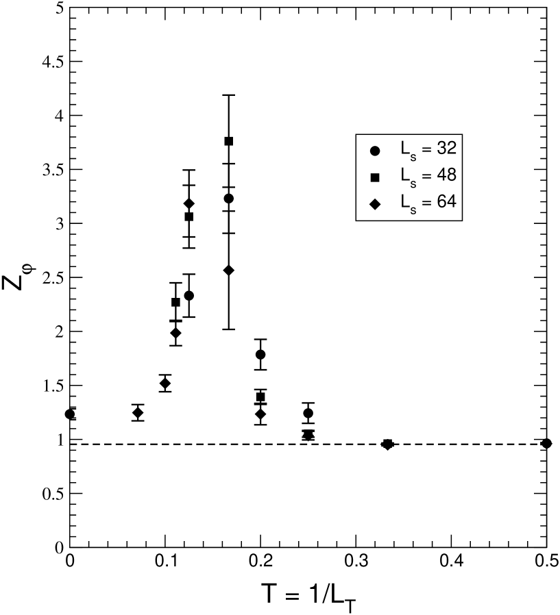
Figure 5: The lattice data for $Z_{\varphi}\equiv m^{2}_{\mathrm{latt}}\chi$ for $L_{s}=32,48,64$ vs. the temperature. The dashed line indicates the zero-temperature value $Z_{\mathrm{prop}}=0.9551$ as in Fig.2

References

- [1] M. Consoli and P. M. Stevenson, Z. Phys. C63, 427 (1994).
- [2] A. Agodi, G. Andronico, and M. Consoli, Zeit. Phys. C66, 439 (1995).
- [3] M. Consoli and P. M. Stevenson, Phys. Lett. B391, 144 (1997).
- [4] M. Consoli and P. M. Stevenson, Int. J. Mod. Phys. A15, 133 (2000).
- [5] U. Ritschel, Zeit. Phys. C63, 345 (1994).
- [6] L. I. Schiff, Phys. Rev. 130, 458 (1963).
- [7] T. Barnes and G. I. Ghandour, Phys. Rev. D22, 924 (1980).
- [8] P. M. Stevenson, Phys. Rev. D32, 1389 (1985).
- [9] M. Consoli and A. Ciancitto, Nucl. Phys. B254, 653 (1985).
- [10] P. M. Stevenson and R. Tarrach, Phys. Lett. B176 436 (1986).
- [11] The possibility of using Eq.(9) as an alternative approach to was first discussed by K. Huang, E. Manousakis and J. Polonyi, Phys. Rev. D35, 3187 (1987).
- [12] S. Coleman and E. Weinberg, Phys. Rev. D7, 1888 (1973).
- [13] P. Cea, M. Consoli, L. Cosmai, Mod. Phys. Lett. A13, 2361 (1998); Nucl. Phys. (Proc. Suppl.) B73, 727 (1999).
- [14] P. Cea, M. Consoli, L. Cosmai and P. M. Stevenson, Mod. Phys. Lett. A14, 1673 (1999); P. Cea, M. Consoli, and L. Cosmai Nucl. Phys. (Proc. Suppl.) B83-84, 658 (2000).
- [15] I. Montvay and P. Weisz, Nucl. Phys. B290, 327 (1987).
- [16] R. Fernández, J. Fröhlich, and A. D. Sokal, Random Walks, Critical Phenomena, and Triviality in Quantum Field Theory (Springer-Verlag, Berlin, 1992).
- [17] C. W. Bernard, Phys. Rev. D9, 3312 (1974); L. Dolan and R. Jackiw, Phys. Rev. D9 3320 (1974); S. Weinberg, Phys. Rev. D9 (1974) 3357.
- [18] I. Montvay and G. Münster, Quantum Fields on a Lattice, Cambridge University Press, 1994.
- [19] R. H. Swendsen and J.-S. Wang, Phys. Rev. Lett. 58, 86 (1987).
- [20] N. Madras and A. D. Sokal, J. Stat. Phys. 50, 109 (1988).
- [21] C. Whitmer, Phys. Rev. D29, 306 (1984); H. Flyvbjerg and H. G. Petersen, J. Chem. Phys. 91, 461 (1989).
- [22] B. Efron, Jackknife, the Bootstrap and Other Resampling Plans, (SIAM Press, Philadelphia, 1982); B. A. Berg and A. H. Billoire, Phys. Rev. D40, 550 (1989).
- [23] M. Lüscher and P. Weisz, Nucl. Phys. B290, 25 (1987); B295, 65 (1988).
- [24] K. Jansen, J. Jersák, I. Montvay, G. Münster, T. Trappenberg and U. Wolff, Phys. Lett. B213, 203 (1988); K. Jansen, I. Montvay, G. Münster, T. Trappenberg and U. Wolff, Nucl. Phys. B322, 698 (1989).
- [25] P. Cea, M. Consoli and L. Cosmai, in preparation.