HIGH-ENERGY QCD AND WILSON LINES

Abstract

At high energies the particles move very fast so their trajectories can be approximated by straight lines collinear to their velocities. The proper degrees of freedom for the fast gluons moving along the straight lines are the Wilson-line operators – infinite gauge factors ordered along the straight line. I review the study of the high-energy scattering in terms of Wilson-line degrees of freedom.

1 Introduction

Traditionally, high-energy scattering in perturbative QCD (pQCD) is studied by direct summation of Feynman diagrams. In the leading logarithmic approximation (LLA)

$$\alpha_{s}\ll 1,\qquad\alpha_{s}\ln{s\over m^{2}}\simeq 1~{},$$ (1)

the amplitudes at high energy are determined by the Balitsky-Fadin-Kuraev-Lipatov (BFKL) pomeron [1] (for a review, see Ref. 2),

$$A(s)\sim\left({s\over m^{2}}\right)^{12{\alpha_{s}\over\pi}\ln 2}\,.$$ (2)

Here $m$ is the characteristic mass or virtuality of scattered particles (for example, for the small-$x$ deep inelastic scattering $m^{2}=Q^{2}$). In order for perturbative QCD (pQCD) to be applicable, $m$ must be sufficiently large so that $\alpha_{s}(m)\ll 1$.

The power behavior of BFKL cross section (2) violates the Froissart bound and, therefore, the BFKL pomeron describes only the pre-asymptotic behavior at intermediate energies when the cross sections are small in comparison to the geometric cross section $2\pi R^{2}$. In order to find the true high-energy asymptotics by analysis of Feynman diagrams we should sum up not only the leading logarithms $(\alpha_{s}\ln s)^{n}$ but also the sub-leading ones $\alpha_{s}(\alpha_{s}\ln s)^{n}$, then the sub-sub-leading terms $\alpha_{s}^{2}(\alpha_{s}\ln s)^{n}$, etc. This is almost equivalent to finding an exact answer to arbitrary QCD amplitude in all orders in perturbation theory. A more realistic approach is to unitarize the BFKL pomeron, i.e. to sum up the subset of sub-leading logarithms which restores the unitarity in $s$ channel. Still, it is a difficult problem which has been in a need of a solution for more than 20 years. One of the most popular ideas on solving this problem is reducing QCD at high energies to some sort of low-dimensional effective theory which will be simpler than original QCD, maybe even to the extent of exact solvability. The first step on this road is to identify proper degrees of freedom for this effective theory. One of the possible choices is to formulate high-energy scattering in terms of “reggeized gluons.”[2] An alternative and related approach [35] is based on so-called Wilson lines – infinite gauge links corresponding to fast gluons moving along the straight-line classical trajectories.

An important aspect of the Wilson-line approach to high-energy scattering is the fact that it serves as a bridge between pQCD calculations and the semiclassical approach to high-energy scattering based on the solution of the classical equations for the fast-moving sources.[4] The semiclassical QCD (sQCD) is applicable when the coupling constant is small but the characteristic fields produced by colliding particles are large, $\sim{1\over g}$. As advocated in Ref. 4, sQCD may be relevant for the heavy-ion collisions because the coupling constant can be relatively small due to high density of partons in the center of the collision. The relevant “saturation scale” was estimated to be $\sim 1$ GeV at RHIC and $\sim 2-3$ GeV at LHC.[5, 6, 7]

Let us demonstrate that the relevant degrees of freedom for the high-energy scattering are Wilson lines.[8] As a result of the high-energy collision, we have a shower of produced particles in the range of rapidity between those of the colliding particles. Consider two clusters of particles with different rapidities: “A” particles with rapidities close to $\eta_{A}$ and “B” particles with rapidities $\simeq\eta_{B}$. From the viewpoint of the “B” particles the “A” gluon moves very fast, so its trajectory can be approximated by a straight line collinear to the gluon momentum, see Fig. 1.

Figure 1: Propagator of a fast “A” gluon in the slow “B” background.

The propagator of such gluon reduces to the free propagator multiplied by the infinite gauge factor (made from “B” gluons) ordered along the straight line parallel to $n_{A}$, the direction corresponding to the rapidity $\eta_{A}$:

$$U(x,n_{A})=[\infty n_{A}+x,-\infty n_{A}+x].$$ (3)

Hereafter we use the notation

$$[x,y]\equiv P\exp ig\int_{0}^{1}du(x-y)^{\mu}A_{\mu}(ux+(1-u)y)$$ (4)

for the straight-line gauge link connecting the points $x$ and $y$. Therefore, the $B$ particles can interact with $A$ fields only via the Wilson lines (3). Similarly, if we sit in the rest frame of the “A” gluons the “B” particles are moving fast along the direction collinear to the vector $n_{B}$ corresponding to rapidity $\eta_{B}$, see Fig. 2.

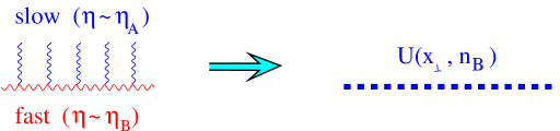
Figure 2: Gluon of “B” type viewed from the rest frame of “A” gluons.

The propagator of these gluons reduces to the Wilson line (made from “A” gluons) collinear to $n_{B}$

$$U(x,n_{B})=[\infty n_{B}+x,-\infty n_{B}+x].$$ (5)

Again, the relevant degree of freedom is the non-local Wilson line (5) rather than the local field $A(x)$. We see that the particles with different rapidities perceive each other as Wilson lines. The formal proof of this statement in terms of Feynman diagrams is given in the Appendix (see also Ref. 9).

In this review I give a pedagogical introduction to the Wilson-line-based approach to high energy scattering. After a short overview of the traditional approach, I shall present the operator expansion for high-energy scattering which provides the operator language for the BFKL equation in the same way as the usual light-cone expansion gives the operator description of the DGLAP equation. Unlike the latter, there is a symmetry between the coefficient functions and matrix elements in the high-energy operator expansion which can be summarized by the factorization formula for high-energy scattering. This factorization formula gives us the rigorous definition of the effective action for a given interval of rapidity. In the last section we discuss the semiclassical approach to effective action related to the problem of scattering of two shock waves in QCD.

2 The hard pomeron in pQCD

Since there are many excellent reviews of the traditional, Feynman diagrams-based, approach to high-energy scattering (see e.g. Refs. 2, 10), I will present here the short introduction to the subject so as to set up the stage for the subsequent analysis of the high-energy scattering in terms of Wilson-line operators.

2.1 High-energy $\gamma^{\ast}\gamma^{\ast}$ scattering

For simplicity, we consider the classical example of high-energy scattering of virtual photons with virtualities $\sim-~{}m^{2}$

$$A(s,t)=-i\int d^{4}xd^{4}yd^{4}ze^{-ip_{A}x-ip_{B}y+ip^{\prime}_{A}z}{\mbox{$\langle 0|$}}T\{j_{A}(x)j_{B}(y)j^{\prime}_{A}(z)j^{\prime}_{B}(0)\}{\mbox{$|0\rangle$}}.$$ (6)

Here $j_{A}(x)$ is electromagnetic current $j^{\mu}(x)$ multiplied by the polarization vector $e^{A}_{\mu}(p)$. In the Regge limit ($s\gg m^{2},t$) it is convenient to use the Sudakov decomposition:

$$p^{\mu}~{}=~{}\alpha_{p}p_{1}^{\mu}+\beta_{p}p_{2}^{\mu}+p_{\perp}^{\mu},$$ (7)

where $p_{1}^{\mu}$ and $p_{2}^{\mu}$ are the light-like vectors close to $p_{A}$ and $p_{B}$, respectively:

$$p_{A}=p_{1}+{p_{A}^{2}\over s}p_{2},\quad p_{B}=p_{2}+{p_{B}^{2}\over s}p_{1},\quad r\equiv p_{B}-p^{\prime}_{B}=\alpha_{r}p_{1}+\beta_{r}p_{2}+r_{\perp}.$$ (8)

The momentum transfer $r=p^{\prime}_{A}-p_{A}=\alpha_{r}p_{1}+\beta_{r}p_{2}+r_{\perp}$ has components $\alpha_{r}\sim\beta_{r}\sim{m^{2}\over s}$ so $t\simeq-{\vec{r}}^{2}$. The typical diagram for the high-energy $\gamma^{\ast}\gamma^{\ast}$ amplitude is shown in Fig. 3 (recall that the diagrams with gluon exchanges dominate at high energies).

Figure 3: A typical Feynman diagram for the high-energy $\gamma^{*}\gamma^{*}$ scattering.

We will calculate the imaginary part of the amplitude $A(s,t)$

$$W={1\over\pi}{\rm Im}A.$$ (9)

The real part of $A(s,t)$ can be restored using the dispersion relations. (It turns out that in the leading logarithmic approximation (LLA) the amplitude at high energy is purely imaginary, see e.g. the review in Ref. 2).

Let us start with the lowest-order diagrams shown in Fig. 4. The integral over gluon momentum $k=\alpha_{k}p_{1}+\beta_{k}p_{2}+k_{\perp}$ has the form

$$W^{0}={2\over\pi}g^{4}\int{d^{4}k\over 16\pi^{4}}{1\over k^{2}}{1\over(r-k)^{2}}{\rm Im}(\Phi_{A})^{ab}_{\xi\eta}(k,+r-k){\rm Im}\Phi_{B}^{\xi\eta ab}(-k,k-r)$$ (10)

where $(\Phi_{A})^{ab}_{\xi\eta}(k,r-k)$ and $(\Phi_{B})^{ab}_{\xi\eta}(-k,k-r)$ are the upper and the lower blocks of the diagram in Fig. 4 (stripped of the strong coupling constant $g$). Here $a,b$ and $\xi,\eta$ are the color and Lorentz indices, respectively.

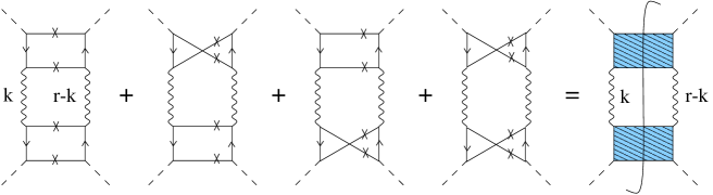
Figure 4: Lowest-order diagrams for the high-energy scattering of virtual photons.

In the Regge kinematics ($\equiv~{}s\gg$ everything else) $\alpha_{k}\sim{m^{2}\over s}$ and $\beta_{k}\sim x$ so $k^{2}\simeq-\vec{k}_{\perp}^{2}$. Moreover, alpha’s in the upper block are $\sim 1$ so one can drop $\alpha_{k}$ in the upper block. Similarly, beta’s in the lower block are $\sim 1$ hence one can neglect $\beta_{k}$ in the lower block. We get ($\Phi^{ab}={\delta_{ab}\over N_{c}^{2}-1}\Phi^{cc}$)

$$W^{0} = {2g^{4}\over(N_{c}^{2}-1)\pi}$$

$$\times \int{d^{4}k\over 16\pi^{4}}{1\over\vec{k}_{\perp}^{2}}{1\over(\vec{r}-\vec{k})_{\perp}^{2}}{\rm Im}\left.\Phi^{aa}_{\xi\eta}(k,r-k)\right|_{\alpha_{k}=0}{\rm Im}\left.\Phi^{\xi\eta bb}(-k,k-r)\right|_{\beta_{k}=0},$$

where $N_{c}=3$ is the number of colors. At high energies, the metric tensor $g^{\mu\nu}$ in the numerator of the Feynman-gauge gluon propagator reduces to ${2\over s}p_{2}^{\mu}p_{1}^{\nu}$, so the integral (2.1) for the imaginary part factorizes into a product of two “impact factors” integrated with two-dimensional propagators

$$W^{0}={s\over\pi}g^{4}{N_{c}^{2}-1\over 4}\left(\sum e_{q}^{2}\right)^{2}\int{d^{2}k_{\perp}\over 4\pi^{2}}{1\over\vec{k}_{\perp}^{2}}{1\over(\vec{r}-\vec{k})_{\perp}^{2}}I^{A}(k_{\perp},r_{\perp})I^{B}(-k_{\perp},-r_{\perp}),$$ (12)

where

$$I^{A}(k_{\perp},r_{\perp})\!\!\!\!\! = \!\!\!\!\!{p_{2}^{\xi}p_{2}^{\eta}\over s(N_{c}^{2}-1)}\left(\sum e_{q}^{2}\right)^{-1}\left.\int{d\beta_{k}\over 2\pi}{\rm Im}\Phi^{aa}_{\xi\eta}(k,r-k)\right|_{\alpha_{k}=0},$$ (13)

$$I^{B}(-k_{\perp},-r_{\perp})\!\!\!\!\! = \!\!\!\!\!{p_{1}^{\xi}p_{1}^{\eta}\over s(N_{c}^{2}-1)}\left(\sum e_{q}^{2}\right)^{-1}\left.\!\!\!\!\int\!\!{d\alpha_{k}\over 2\pi}{\rm Im}\Phi^{aa}_{N\xi\eta}(-k,k-r)\right|_{\beta_{k}=0},$$ (14)

and $\left(\sum e_{q}^{2}\right)$ is the sum of squared charges of active flavors. The photon impact factor is given by the two one-loop diagrams shown in Fig. 5.

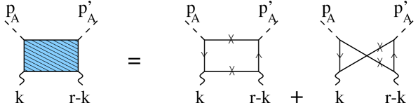
Figure 5: Photon impact factor.

The standard calculation of these diagrams yields [11]

$${I}^{A}(k_{\perp},r_{\perp})=\bar{I}^{A}(k_{\perp},r_{\perp})-\bar{I}^{A}(0,r_{\perp}),$$ (15)

where

$$\bar{I}^{A}(k_{\perp},r_{\perp}) = {1\over 2}\int_{0}^{1}\frac{d\alpha}{2\pi}\int_{0}^{1}\frac{d\alpha^{\prime}}{2\pi}\left\{\vec{P}_{\perp}^{2}\alpha^{\prime}\bar{\alpha^{\prime}}-[p_{A}^{2}\bar{\alpha}^{\prime}+(p^{\prime}_{A})^{2}\alpha^{\prime}]\alpha\bar{\alpha}\right\}^{-1}$$

$$\times \Bigg{\{}(1-2\alpha\bar{\alpha})(1-2\alpha^{\prime}\bar{\alpha}^{\prime})\vec{P}_{\perp}^{2}(\vec{e}_{A},\vec{e}^{\prime}_{A})_{\perp}+4\alpha\bar{\alpha}\alpha^{\prime}\bar{\alpha^{\prime}}[\vec{P}_{\perp}^{2}(\vec{e}_{A},\vec{e}^{\prime}_{A})_{\perp}$$

$$- 2(\vec{P},\vec{e}_{A})_{\perp}(\vec{P},\vec{e}^{\prime}_{A})_{\perp}]+(e_{A},e^{\prime}_{A})_{\perp}(p_{A}^{2}-(p^{\prime}_{A})^{2})\alpha\bar{\alpha}(1-2\alpha\bar{\alpha})$$

$$\times (1-2\alpha^{\prime})+4\alpha\bar{\alpha}(1-2\alpha)\alpha^{\prime}(\vec{P},\vec{e}_{A})_{\perp}(\vec{r},\vec{e}^{\prime}_{A})_{\perp}\Bigg{\}}$$

for the transverse polarizations $A,A^{\prime}=1,2$. Here $P_{\perp}\equiv k_{\perp}-r_{\perp}\alpha$ and $(a,b)_{\perp}$ denotes the (positive) scalar product of transverse components of vectors $a$ and $b$.

2.2 The BFKL kernel

In the next order in perturbation theory there are two types of diagrams for the $\gamma^{*}\gamma^{*}$ amplitude: diagrams with 5-particle cut describing the emission of an extra gluon and diagrams with 4-particle cut as in Fig. 4 but with an extra gluon loop.

Let us at first consider the diagrams with the 5-particle cut shown in Fig. 6.

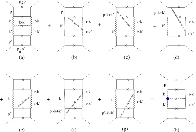
Figure 6: The effective vertex in LLA.

The contribution of the diagram shown in Fig. 6a has the form

$$W_{(a)}^{(5)} = {2\over\pi}g^{6}\int{d^{4}k\over 16\pi^{4}}\int{d^{4}k^{\prime}\over 16\pi^{4}}{{\rm Im}\Phi_{A}^{\mu\nu ab}(k,r-k)\over k^{2}(r-k)^{2}}{{\rm Im}\Phi_{B}^{\xi\eta mn}(-k^{\prime},k^{\prime}-r)\over(k^{\prime})^{2}(r-k^{\prime})^{2}}$$ (17)

$$\times f^{amc}f^{bnc}\Gamma_{\mu\xi}^{~{}~{}~{}\sigma}(k,k^{\prime})2\pi\delta((k-k^{\prime})^{2})\theta(\alpha_{k})\Gamma_{\nu\eta\sigma}(r-k,r-k^{\prime})$$

$$\times {{\rm Im}\Phi_{B}^{\xi\eta mn}(-k^{\prime},k^{\prime}-r)\over(k^{\prime})^{2}(r-k^{\prime})^{2}},$$

where

$$\Gamma_{\mu\nu\lambda}(k,k^{\prime})=(k+k^{\prime})_{\lambda}g_{\mu\nu}+(k^{\prime}-2k)_{\nu}g_{\lambda\mu}+(k-2k^{\prime})_{\mu}g_{\nu\lambda}$$ (18)

is the three-gluon vertex divided by g. (Strictly speaking, in order to obtain $\Phi^{A}$ and $\Phi^{B}$ we must add the diagrams with permutations of the quark lines, as in Fig. 4). As mentioned above, it is convenient to use Sudakov variables (7): $k=\alpha_{k}p_{1}+\beta_{k}p_{2}+k_{\perp}$, $k^{\prime}=\alpha^{\prime}_{k}p_{1}+\beta^{\prime}_{k}p_{2}+k^{\prime}_{\perp}$. We will see that the logarithmic contribution comes from the region

$$1\gg\alpha\gg\alpha^{\prime}\sim{m^{2}\over s},~{}~{}~{}{m^{2}\over s}\sim\beta\ll\beta^{\prime}\ll 1,~{}~{}~{}\vec{k}_{\perp}^{2}\sim(k^{\prime}_{\perp})^{2}\sim m^{2}.$$ (19)

In this region $k^{2}=\alpha_{k}\beta_{k}s-\vec{k}_{\perp}^{2}\simeq-\vec{k}_{\perp}^{2}$. In the same way, $(k^{\prime})^{2}=-(\vec{k}^{\prime}_{\perp})^{2}$, $(r-k)^{2}=-(\vec{r}-\vec{k})_{\perp}^{2}$, and $(r-k^{\prime})^{2}=-(\vec{r}-\vec{k}^{\prime})_{\perp}^{2}$. As we mentioned above, at high energies we can replace $g^{\mu\nu}$ in gluon propagators connecting the clusters with different rapidities by $2{p_{2}^{\mu}p_{1}^{\nu}\over s}$. With these approximations, the integral (17) reduces to

$$W_{(a)}^{(5)} = \!{2\over\pi}g^{6}\Big{(}{2\over s}\Big{)}^{4}\int{d\alpha_{k}d\beta_{k}\over 4\pi^{2}}{d^{2}k_{\perp}\over 4\pi^{2}}\int{d\alpha^{\prime}_{k}d\beta^{\prime}_{k}\over 4\pi^{2}}{d^{2}k^{\prime}_{\perp}\over 4\pi^{2}}{1\over\vec{k}_{\perp}^{2}}{1\over(\vec{r}-\vec{k})_{\perp}^{2}}$$ (20)

$$\times \!{\rm Im}\Phi_{A}^{\ast\ast ab}(k,r-k)f^{amc}f^{bnc}\Gamma_{\bullet\ast}^{~{}~{}~{}\sigma}(k,k^{\prime})2\pi\delta(\alpha_{k}\beta^{\prime}_{k}s+(\vec{k}-\vec{k}^{\prime})_{\perp}^{2})\theta(\alpha_{k})$$

$$\times \!\Gamma_{\bullet\ast\sigma}(r-k,r-k^{\prime}){1\over(\vec{k}^{\prime})_{\perp}^{2}}{1\over(\vec{r}-\vec{k}^{\prime})_{\perp}^{2}}{\rm Im}\Phi_{B}^{\bullet\bullet mn}(-k^{\prime},k^{\prime}-r).$$

Since $\alpha$ in the upper block is $\sim 1$, one can neglect $\alpha_{k}$-dependence in $\Phi_{A}$ which leads to the replacement of $\int d\beta_{k}\Phi_{A}$ by the impact factor $I^{A}(k_{\perp},r_{\perp})$, see Eq. (2.1). Likewise, $\int d\alpha^{\prime}_{k}\Phi_{B}\rightarrow I^{B}(k^{\prime}_{\perp},r_{\perp})$ so we get

$$W_{(a)}^{(5)} = {2g^{6}\over\pi}{N_{c}(N_{c}^{2}-1)\over 4}\left(\sum e_{q}^{2}\right)^{2}$$ (21)

$$\times\!\!\!\!\! \int{d^{2}k_{\perp}\over 4\pi^{2}}{d^{2}k^{\prime}_{\perp}\over 4\pi^{2}}I^{A}(k_{\perp},r_{\perp}){1\over\vec{k}_{\perp}^{2}(\vec{r}-\vec{k})_{\perp}^{2}}{1\over(\vec{k}^{\prime})_{\perp}^{2}(\vec{r}-\vec{k}^{\prime})_{\perp}^{2}}I^{B}(k^{\prime}_{\perp},r_{\perp})$$

$$\times\!\!\!\!\! \int{d\alpha_{k}d\beta^{\prime}_{k}\over 4\pi^{2}}\Gamma_{\bullet\ast}^{~{}~{}~{}\sigma}(k,k^{\prime})2\pi\delta(\alpha_{k}\beta^{\prime}_{k}s+(\vec{k}-\vec{k}^{\prime})_{\perp}^{2})\theta(\alpha_{k})\Gamma_{\bullet\ast;\sigma}(r-k,r-k^{\prime}).$$

Let us now turn to the diagram shown in Fig. 6b. Since the gluon with momentum $k-k^{\prime}$ now connects parts of the diagrams with different rapidities, we can replace $g^{\mu\nu}$ in this propagator by $2{p_{2}^{\mu}p_{1}^{\nu}\over s}$. After that, the quark propagator with the momentum $p+k^{\prime}$ in the upper block reduces to

$$t^{a}{\not\!p}_{2}{(\alpha_{p}+\alpha^{\prime}_{k}){\not\!p}_{1}+{\not\!p}_{\perp}+{\not\!k^{\prime}}_{\perp}\over-(\alpha_{p}+\alpha^{\prime}_{k})(\beta_{p}+\beta^{\prime}_{k})s+(\vec{p}-\vec{k}^{\prime})_{\perp}^{2}-i\epsilon}{\not\!p}_{2}t^{c}\rightarrow t^{a}{\not\!p}_{2}{1\over-\beta^{\prime}_{k}-i\epsilon}t^{c},$$ (22)

(recall that $\alpha_{p}\sim 1,\beta_{p}\sim{m^{2}\over s}$). We see that in the transverse space this propagator shrinks to a point so the answer for the upper block is again $I^{A}$ multiplied by ${1\over\beta^{\prime}_{k}+i\epsilon}$. (The eikonal factor ${1\over\beta^{\prime}_{k}+i\epsilon}$ is the Fourier transform of the first term of the expansion of Wilson-line propagator (3) in powers of “external slow field” represented by gluon with momentum $k^{\prime}$). The right part of the diagram in Fig. 6b is identical to that in Fig. 6a so we obtain

$$W_{(b)}^{(5)} = i{2\over\pi}g^{6}{\rm Tr}\{t^{a}t^{c}t^{b}\}\int{d^{2}k_{\perp}\over 4\pi^{2}}\int{d\alpha_{k}d\beta^{\prime}_{k}\over 4\pi^{2}}{d^{2}k^{\prime}_{\perp}\over 4\pi^{2}}I^{A}(k_{\perp},r_{\perp})f^{bac}$$

$$\times {1\over\beta^{\prime}_{k}}{1\over(\vec{r}-\vec{k})_{\perp}^{2}}2\pi\delta(\alpha_{k}\beta^{\prime}_{k}s+(\vec{k}-\vec{k}^{\prime})_{\perp}^{2})\theta(\alpha_{k})\Gamma_{\bullet\ast\bullet}(r-k,r-k^{\prime})$$

$$\times {1\over(\vec{k}^{\prime})_{\perp}^{2}}{1\over(\vec{r}-\vec{k}^{\prime})_{\perp}^{2}}I^{B}(k^{\prime}_{\perp},r_{\perp}).$$

The contribution of the diagram in Fig. 6c is calculated in a similar way. One can replace

$${t^{c}{\not\!p}_{2}\big{[}(\alpha_{p}-\alpha_{k}+\alpha^{\prime}_{k}){\not\!p}_{1}+{\not\!p}_{\perp}-{\not\!k}_{\perp}+{\not\!k^{\prime}}_{\perp}{\not\!p}_{2}t^{a}\big{]}\over(\alpha_{p}-\alpha_{k}+\alpha^{\prime}_{k})(\beta_{p}-\beta_{k}+\beta^{\prime}_{k})s-(\vec{p}-\vec{k}+\vec{k}^{\prime})_{\perp}^{2}+i\epsilon}\rightarrow t^{c}{\not\!p}_{2}{1\over\beta^{\prime}_{k}-i\epsilon}t^{a},$$ (24)

and, therefore,

$$W_{(c)}^{(5)} = -i{2\over\pi}g^{6}{\rm Tr}\{t^{b}t^{a}t^{c}\}\int{d^{2}k_{\perp}\over 4\pi^{2}}\int{d\alpha_{k}d\beta^{\prime}_{k}\over 4\pi^{2}}{d^{2}k^{\prime}_{\perp}\over 4\pi^{2}}I^{A}(k_{\perp},r_{\perp})f^{abc}$$

$$\times {1\over\beta^{\prime}_{k}}{1\over(\vec{r}-\vec{k})_{\perp}^{2}}2\pi\delta(\alpha_{k}\beta^{\prime}_{k}s+(\vec{k}-\vec{k}^{\prime})_{\perp}^{2})\theta(\alpha_{k})\Gamma_{\bullet\ast\bullet}(r-k,r-k^{\prime})$$

$$\times {1\over(\vec{k}^{\prime})_{\perp}^{2}}{1\over(\vec{r}-\vec{k}^{\prime})_{\perp}^{2}}I^{B}(k^{\prime}_{\perp},r_{\perp}).\$$

Note that the sum of the results (21), (2.2), and (2.2) may be obtained from the contribution (21) of the diagram in Fig. 6a. by the replacement

$$\Gamma_{\bullet\ast}^{~{}~{}\sigma}(k,k^{\prime})\rightarrow\Gamma_{\bullet\ast}^{~{}~{}\sigma}(k,k^{\prime})-{\vec{k}_{\perp}^{2}\over\beta^{\prime}_{k}}p_{2}^{\sigma}.$$ (26)

Now consider now the the diagram in Fig. 6d. The two quark propagators carrying the momentum $k^{\prime}$ give

$${\not\!p}_{2}{(1-\alpha_{p}+\alpha^{\prime}_{k}){\not\!p}_{1}-{\not\!p}_{\perp}+{\not\!k^{\prime}}_{\perp}\over(1-\alpha_{p}+\alpha^{\prime}_{k})({m^{2}\over s}-\beta_{p}+\beta^{\prime}_{k})s-(\vec{p}-\vec{k}^{\prime})_{\perp}^{2}+i\epsilon}$$ (27)

$$\times \not\!e^{A}_{\perp}{(\alpha_{p}+\alpha^{\prime}_{k}){\not\!p}_{1}+{\not\!p}_{\perp}+{\not\!k^{\prime}}_{\perp}\over(\alpha_{p}+\alpha^{\prime}_{k})(\beta_{p}+\beta^{\prime}_{k})s-(\vec{p}-\vec{k}^{\prime})_{\perp}^{2}+i\epsilon}{\not\!p}_{2}$$

$$\rightarrow {\not\!p}_{2}{(1-\alpha_{p}){\not\!p}_{1}-{\not\!p}_{\perp}+{\not\!k^{\prime}}_{\perp}\over(1-\alpha_{p})\beta^{\prime}_{k}s}e^{A}_{\perp}{(\alpha_{p}+\alpha^{\prime}_{k}){\not\!p}_{1}+{\not\!p}_{\perp}+{\not\!k^{\prime}}_{\perp}\over\alpha_{p}\beta^{\prime}_{k}s}.$$

Since we cannot keep both large terms $(1-\alpha_{p})p_{1}$ and $\alpha_{p}p_{1}$ in the numerators this expression is ${m^{2}\over\beta^{\prime}_{k}s}$ times smaller than the contribution (2.2) of the diagram in Fig. 6b so it vanishes in the LLA.

The diagrams in Fig 6e,f are calculated in the same way as the diagrams in Fig 6b,c. Similarly, the result may be obtained from Eq. (21) by the replacement

$$\Gamma_{\bullet\ast}^{~{}~{}\sigma}(k,k^{\prime})\rightarrow-{(\vec{k}^{\prime})_{\perp}^{2}\over\alpha_{k}s}p_{1}^{\sigma}.$$ (28)

In conclusion, the diagram in Fig. 6g vanishes in the LLA for the same reasons as the Fig. 6c diagram.

Thus, the contribution of the diagrams in Fig. 6a–6e can be represented by one diagram shown in Fig. 6h:

$$W_{(a+...g)}^{(5)}~{}=~{}{sg^{6}\over\pi}{N_{c}(N_{c}^{2}-1)\over 4}\left(\sum e_{q}^{2}\right)^{2}$$ (29)

$$\times~{}\int{d^{2}k_{\perp}\over 4\pi^{2}}{d^{2}k^{\prime}_{\perp}\over 4\pi^{2}}I^{A}(k_{\perp},r_{\perp}){1\over\vec{k}_{\perp}^{2}(\vec{r}-\vec{k})_{\perp}^{2}}{1\over(\vec{k}^{\prime})_{\perp}^{2}(\vec{r}-\vec{k}^{\prime})_{\perp}^{2}}I^{B}(k^{\prime}_{\perp},r_{\perp})$$

$$\times~{}\int{d\alpha_{k}d\beta^{\prime}_{k}\over 4\pi^{2}}L^{\sigma}(k,k^{\prime})2\pi\delta(\alpha_{k}\beta^{\prime}_{k}s+(\vec{k}-\vec{k}^{\prime})_{\perp}^{2})\theta(\alpha_{k})\Gamma_{\bullet\ast\sigma}(r-k,r-k^{\prime}),$$

where

$$L^{\sigma}(k,k^{\prime}) = {2\over s}\Gamma_{\bullet\ast}^{\sigma}(k,k^{\prime})-2{(\vec{k}_{\perp})^{2}\over\beta^{\prime}_{k}s}p_{2}^{\sigma}-2{(\vec{k}^{\prime}_{\perp})^{2}\over\alpha_{k}s}p_{1}^{\sigma}$$ (30)

$$= (k+k^{\prime})_{\perp}^{\sigma}-(\alpha_{k}+2{\vec{k}_{\perp}^{2}\over\beta^{\prime}_{k}s})p_{1}^{\sigma}-(\beta^{\prime}_{k}+2{(\vec{k}^{\prime})_{\perp}^{2}\over\alpha_{k}s})p_{2}^{\sigma}$$

is the Lipatov effective vertex for the gluon emission shown in Fig. 6h by a shaded circle. Note that unlike the usual three-gluon vertex, the effective vertex is gauge-invariant,

$$(k-k^{\prime})_{\sigma}L^{\sigma}(k,k^{\prime})=0.$$ (31)

We have demonstrated that if we take the diagram in Fig. 6a and attach the left end of the $k-k^{\prime}$ gluon line in all possible ways, the left three-gluon vertex in Fig. 6a is replaced by the effective vertex (30). Likewise, the sum of all possible attachments of the right end of this $k-k^{\prime}$ gluon line converts the right three-gluon vertex $\Gamma_{\bullet\ast\sigma}(r-k,r-k^{\prime})$ into the effective vertex $L_{\sigma}(r-k,r-k^{\prime})$. Hence the sum of all the diagrams with 5-particle cut takes the form (see Fig. 7)

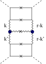
Figure 7: Sum of the diagrams with gluon emission in LLA. Shaded circle denotes the effective vertex.

$$W^{(5)} = {g^{6}\over\pi}{N_{c}(N_{c}^{2}-1)\over 4}\left(\sum e_{q}^{2}\right)^{2}{s^{2}\over 2}$$

$$\times \int{d^{2}k_{\perp}\over 4\pi^{2}}{d^{2}k^{\prime}_{\perp}\over 4\pi^{2}}{I^{A}(k_{\perp},r_{\perp})I^{B}(k^{\prime}_{\perp},r_{\perp})\over\vec{k}_{\perp}^{2}(\vec{r}-\vec{k})_{\perp}^{2}(\vec{k}^{\prime})_{\perp}^{2}(\vec{r}-\vec{k}^{\prime})_{\perp}^{2}}$$

$$\times \int{d\alpha_{k}d\beta^{\prime}_{k}\over 4\pi^{2}}L^{\sigma}(k,k^{\prime})2\pi\delta(\alpha_{k}\beta^{\prime}_{k}s+(\vec{k}-\vec{k}^{\prime})_{\perp}^{2})\theta(\alpha_{k})L_{\sigma}(r-k,r-k^{\prime}).$$

Since $\alpha_{k}\beta^{\prime}_{k}s=-(\vec{k}-\vec{k}^{\prime})_{\perp}^{2}$ due to the $\delta$-function, the product of two Lipatov’s vertices gives

$${1\over 2}L^{\sigma}(k,k^{\prime})L_{\sigma}(r-k,r-k^{\prime})=-\vec{r}_{\perp}^{2}+{\vec{k}_{\perp}^{2}(\vec{r}-\vec{k}^{\prime})_{\perp}^{2}\over(\vec{k}-\vec{k}^{\prime})_{\perp}^{2}}+{(\vec{k}^{\prime})_{\perp}^{2}(\vec{r}-\vec{k})_{\perp}^{2}\over(\vec{k}-\vec{k}^{\prime})_{\perp}^{2}},$$ (33)

which is proportional to the “emission” part of the BFKL kernel, see the Eq. (36) below. Now one can easily perform the remaining integrations over $\alpha_{k}$ and $\beta^{\prime}_{k}$ in the LLA

$$s\!\int\!d\alpha_{k}d\beta^{\prime}_{k}\delta(\alpha_{k}\beta^{\prime}_{k}s+(\vec{k}-\vec{k}^{\prime})_{\perp}^{2})\theta(\alpha_{k})=\int^{1}_{m^{2}\over s}d\alpha_{k}{1\over\alpha_{k}}=\ln{s\over m^{2}},$$ (34)

and, therefore, the final result (for the diagrams with 5-particle cut) is

$$W^{(5)} = {s\over\pi}g^{4}{N_{c}^{2}-1\over 4}{g^{2}\over 2\pi}N_{c}\ln{s\over m^{2}}$$

$$\times \int{d^{2}k\over 4\pi^{2}}{d^{2}k^{\prime}\over 4\pi^{2}}I^{A}(k_{\perp},r_{\perp}){1\over\vec{k}_{\perp}^{2}(\vec{r}-\vec{k})_{\perp}^{2}}K_{1}(k_{\perp},k_{\perp}^{\prime},r)I^{B}(k^{\prime}_{\perp},r_{\perp})$$

where

$$K_{(1)}(k_{\perp},k_{\perp}^{\prime},r)=-{\vec{r}_{\perp}^{2}\over(\vec{k}^{\prime})_{\perp}^{2}(\vec{r}-\vec{k}^{\prime}_{\perp})^{2}}+{\vec{k}_{\perp}^{2}\over(\vec{k}^{\prime})_{\perp}^{2}(\vec{k}-\vec{k}^{\prime}_{\perp})^{2}}+{(\vec{k}-\vec{r})_{\perp}^{2}\over(\vec{k}^{\prime}-\vec{r})_{\perp}^{2}(\vec{k}-\vec{k}^{\prime}_{\perp})^{2}}$$ (36)

is the first part of the BFKL kernel coming from the diagrams with gluon emission.

Apart from the diagrams with 5-particle cut shown in Fig. 6, there are also diagrams with four-particle cut (“virtual corrections”) of the type shown in Fig. 8.

Figure 8: Virtual corrections.

Let us consider the diagram shown in Fig. 8a. The integrals over $\alpha_{k}$ and $\beta_{k}$ are similar to the same integrals in the first-order diagram in Fig. 4 and therefore $\alpha_{k}\sim\beta_{k}\sim{m^{2}\over s}$. The logarithmic contribution comes from the region $1\sim\alpha_{p}\gg\alpha^{\prime}_{k}\gg\alpha_{k}$. In this region we can replace the quark propagator with momentum $p-k^{\prime}$ by the eikonal propagator (see Appendix 7.1),

$$\not\!p_{2}({\not\!p+\not\!k^{\prime}})\not\!p_{2}\rightarrow\not\!p_{2}{1\over-\beta^{\prime}_{k}+i\epsilon}.$$ (37)

In addition, one can neglect $\beta^{\prime}_{k}$ in comparison to $\beta^{\prime}_{p}\sim 1$ in the lower block . The loop integral over $k^{\prime}$ turns into

$$\int{d\alpha^{\prime}_{k}d\beta^{\prime}_{k}\over 4\pi^{2}}{d^{2}k^{\prime}\over 4\pi^{2}}\left[t^{a}{\not\!p_{2}\over-\beta^{\prime}_{k}+i\epsilon}t^{b}\right]{1\over\alpha^{\prime}_{k}\beta^{\prime}_{k}s-\vec{k}_{\perp}^{2}}{1\over\alpha^{\prime}_{k}(\beta^{\prime}_{k}-\beta_{k})-(\vec{k}-\vec{k}^{\prime})_{\perp}^{2}}$$ (38)

$$\times \left[t^{a}{\not\!p_{1}(\beta^{\prime}_{p}\not\!p_{2}+\not\!p^{\prime}_{\perp}+\not\!k^{\prime}_{\perp})\not\!p_{1}\over\alpha^{\prime}_{k}\beta^{\prime}_{p}s-(\vec{p}^{\prime}+\vec{k}^{\prime})^{2}_{\perp}}t^{b}\right].$$

The integral over $\beta^{\prime}_{k}$ is determined by the residue at $\beta^{\prime}_{k}=0$ so we obtain

$$\int_{m^{2}\over s}^{1}{d\alpha^{\prime}_{k}\over 2\pi\alpha^{\prime}_{k}}\int{d^{2}k^{\prime}_{\perp}\over 4\pi^{2}}\Big{[}t^{a}\not\!p_{2}t^{b}\Big{]}{1\over\vec{k}_{\perp}^{2}}{1\over(\vec{k}-\vec{k}^{\prime})_{\perp}^{2}}\Big{[}t^{a}{\not\!p_{1}}t^{b}\Big{]}$$ (39)

$$= \Big{[}t^{a}\not\!p_{2}t^{b}\Big{]}\Big{[}t^{a}{\not\!p_{1}}t^{b}\Big{]}\times{g^{2}\over 4\pi^{2}}\ln{s\over m^{2}}\int{d^{2}k^{\prime}_{\perp}\over 4\pi^{2}}{1\over\vec{k}_{\perp}^{2}}{1\over(\vec{k}-\vec{k}^{\prime})_{\perp}^{2}}.$$

Let us add now the contribution of the diagram in Fig. 8b. Like the Fig. 8a case, we get the loop integral over $k^{\prime}$ in the form

$$\int{d\alpha^{\prime}_{k}d\beta^{\prime}_{k}\over 4\pi^{2}}{d^{2}k^{\prime}\over 4\pi^{2}}\left[t^{a}{\not\!p_{2}\over-\beta^{\prime}_{k}+i\epsilon}t^{b}\right]{1\over\alpha^{\prime}_{k}\beta^{\prime}_{k}s-\vec{k}_{\perp}^{2}}{1\over\alpha^{\prime}_{k}(\beta^{\prime}_{k}-\beta_{k})-(\vec{k}-\vec{k}^{\prime})_{\perp}^{2}}$$ (40)

$$\times \left[t^{a}{\not\!p_{1}(\beta^{\prime}_{p}\not\!p_{2}+\not\!p^{\prime}_{\perp}+\not\!k^{\prime}_{\perp})\not\!p_{1}\over\alpha^{\prime}_{k}\beta^{\prime}_{p}s-(\vec{p}^{\prime}+\vec{k}^{\prime})^{2}_{\perp}}t^{b}\right]$$

$$= \int_{m^{2}\over s}^{1}{d\alpha^{\prime}_{k}\over 2\pi\alpha^{\prime}_{k}}\int{d^{2}k^{\prime}_{\perp}\over 4\pi^{2}}\Big{[}t^{a}\not\!p_{2}t^{b}\Big{]}{1\over\vec{k}_{\perp}^{2}}{1\over(\vec{k}-\vec{k}^{\prime})_{\perp}^{2}}\Big{[}t^{a}{\not\!p_{1}}t^{b}\Big{]}$$

$$= \Big{[}t^{a}\not\!p_{2}t^{b}\Big{]}\Big{[}t^{a}{\not\!p_{1}}t^{b}\Big{]}\times{g^{2}\over 4\pi^{2}}\ln{s\over m^{2}}\int{d^{2}k^{\prime}_{\perp}\over 4\pi^{2}}{1\over(\vec{k}^{\prime})_{\perp}^{2}(\vec{k}-\vec{k}^{\prime})_{\perp}^{2}}.$$

The diagrams shown in Fig. 8c–g do not give the logarithmic contribution for the same reason as the diagram in Fig. 6d.

We see that the sum of diagrams in Fig. 8a–g reduces to the first-order diagram in Fig. 4a with the left gluon propagator ${1\over-\vec{k}_{\perp}^{2}}$ replaced by the factor

$${1\over-\vec{k}_{\perp}^{2}}\rightarrow{g^{2}\over 4\pi}N_{c}\ln{s\over m^{2}}\int{d^{2}k^{\prime}_{\perp}\over 4\pi^{2}}{1\over(\vec{k}^{\prime})_{\perp}^{2}(\vec{k}-\vec{k}^{\prime})_{\perp}^{2}}$$ (41)

shown schematically in Fig. 8h. We get

$$W_{(a+...g)}^{(4)} = -{s\over\pi}g^{4}{N_{c}^{2}-1\over 4}\left(\sum e_{q}^{2}\right)^{2}{g^{2}\over 4\pi}N_{c}\ln{s\over m^{2}}$$

$$\times \int{d^{2}k_{\perp}\over 4\pi^{2}}{I^{A}(k_{\perp},r_{\perp})I_{B}(k_{\perp},r_{\perp})\over{\vec{k}}_{\perp}^{2}(\vec{r}-\vec{k})_{\perp}^{2}}\left\{\int{d^{2}k^{\prime}_{\perp}\over 4\pi^{2}}{\vec{k}^{2}\over(\vec{k}^{\prime})_{\perp}^{2}(\vec{k}-\vec{k}^{\prime})_{\perp}^{2}}\right\}.$$

The diagrams with the gluon loop to the right of the cut lead to similar replacement of the right gluon propagator ${1\over-(\vec{k}-\vec{r})_{\perp}^{2}}$ by

$${1\over-(\vec{k}-\vec{r})_{\perp}^{2}}\rightarrow{g^{2}N_{c}\over 4\pi}\ln{s\over m^{2}}\int{d^{2}k^{\prime}_{\perp}\over 4\pi^{2}}{1\over(\vec{k}^{\prime}_{\perp}-\vec{r}_{\perp})^{2}(\vec{k}-\vec{k}^{\prime})_{\perp}^{2}}.$$ (43)

Thus we obtain the result

$$W^{(4)} = -{s\over\pi}g^{4}{N_{c}^{2}-1\over 4}\left(\sum e_{q}^{2}\right)^{2}{g^{2}\over 4\pi}N_{c}\ln{s\over m^{2}}$$ (44)

$$\times \int{d^{2}k_{\perp}\over 4\pi^{2}}{I^{A}(k_{\perp},r_{\perp})I_{B}(k_{\perp},r_{\perp})\over{\vec{k}}_{\perp}^{2}(\vec{r}-\vec{k})_{\perp}^{2}}$$

$$\times \int{d^{2}k^{\prime}_{\perp}\over 4\pi^{2}}\left\{{\vec{k}^{2}\over(\vec{k}^{\prime})_{\perp}^{2}(\vec{k}-\vec{k}^{\prime})_{\perp}^{2}}+{(\vec{k}-\vec{r})^{2}\over(\vec{k}^{\prime}-\vec{r})_{\perp}^{2}(\vec{k}-\vec{k}^{\prime})_{\perp}^{2}}\right\}$$

for the contribution of the diagrams with 4-particle cut.

Adding the sum of the diagrams with real gluon emission $W^{5}$ we obtain the final result for the $\gamma^{\ast}\gamma^{\ast}$ scattering amplitude in the first order in LLA. It can be represented in the form

$$W^{1} = {s\over\pi}g^{4}{N_{c}^{2}-1\over 4}\left(\sum e_{q}^{2}\right)^{2}{g^{2}\over 2\pi}N_{c}\ln{s\over m^{2}}\int{d^{2}k\over 4\pi^{2}}{d^{2}k^{\prime}\over 4\pi^{2}}$$

$$\times I^{A}(k_{\perp},r_{\perp}){1\over\vec{k}_{\perp}^{2}(\vec{r}-\vec{k})_{\perp}^{2}}K(k_{\perp},k_{\perp}^{\prime},r)I^{B}(k^{\prime}_{\perp},r_{\perp}),$$

where

$$K(k_{\perp},k_{\perp}^{\prime},r)=K_{(1)}(k_{\perp},k_{\perp}^{\prime},r)-{1\over 2}\delta^{(2)}(k-k^{\prime})$$ (46)

$$\times\left\{\int{d^{2}k"_{\perp}\over 4\pi^{2}}{\vec{k}^{2}\over(\vec{k}")_{\perp}^{2}(\vec{k}-\vec{k}")_{\perp}^{2}}+\int{d^{2}k"_{\perp}\over 4\pi^{2}}{(\vec{k}-\vec{r})^{2}\over(\vec{k}"-\vec{r})_{\perp}^{2}(\vec{k}-\vec{k}")_{\perp}^{2}}\right\}$$

is the BFKL kernel.[1] The explicit form of $K$ is

$$K(k_{\perp},k_{\perp}^{\prime},r)~{}=~{}-{\vec{r}_{\perp}^{2}\over\vec{k^{\prime}}_{\perp}^{2}(\vec{r}-\vec{k}^{\prime})_{\perp}^{2}}+{\vec{k}_{\perp}^{2}\over\vec{k^{\prime}}_{\perp}^{2}(\vec{k}-\vec{k}^{\prime})_{\perp}^{2}}+{(\vec{r}-\vec{k})_{\perp}^{2}\over(\vec{r}-\vec{k}^{\prime})_{\perp}^{2}(\vec{k}-\vec{k}^{\prime})_{\perp}^{2}}$$

$$-{1\over 2}\delta^{(2)}(k-k^{\prime})\int{d^{2}k"_{\perp}\over 4\pi^{2}}\left\{{\vec{k}^{2}\over(\vec{k}")_{\perp}^{2}(\vec{k}-\vec{k}")_{\perp}^{2}}+{(\vec{k}-\vec{r})^{2}\over(\vec{k}"-\vec{r})_{\perp}^{2}(\vec{k}-\vec{k}")_{\perp}^{2}}\right\}.$$ (47)

Note that both $W^{(5)}$ and $W^{(4)}$ are IR divergent but their sum $W^{1}$ given by Eq. (2.2) is IR finite. This is the usual Bloch-Nordsieck cancellation between th emission of real gluon in diagrams in Fig. 6 and virtual gluon in Fig. 8.

2.3 Bare pomeron in the LLA

The $\gamma^{\ast}\gamma^{\ast}$ amplitude in the first two orders in perturbation theory may be represented in the operator form as

$$W^{(0+1)}=s{\cal C}\int{d^{2}k\over 4\pi^{2}}I^{A}(k_{\perp},r_{\perp}){1\over\vec{k}_{\perp}^{2}(\vec{r}-\vec{k})_{\perp}^{2}}\Big{(}1+{g^{2}\over 8\pi^{3}}N_{c}\ln{s\over m^{2}}\hat{K}\Big{)}I^{B}(k_{\perp},r_{\perp}),$$ (48)

where ${\cal C}\equiv\alpha_{s}(N_{c}^{2}-1)(\sum e_{q}^{2})^{2}$ and the operator $\hat{K}_{r}$ is defined by its kernel $K(k,k^{\prime},r)$,

$$(\hat{K}_{r}f)(\vec{k}_{\perp})=\int{d^{2}k^{\prime}\over 4\pi^{2}}K(k_{\perp},k_{\perp}^{\prime},r)f(\vec{k}^{\prime}_{\perp}).$$ (49)

We can demonstrate (and we will do this using the evolution equations for the Wilson-line operators) that in the next orders in LLA the operator $K$ exponentiates:

$$W^{\rm LLA}=s{\cal C}\int{d^{2}k\over 4\pi^{2}}I^{A}(k_{\perp},r_{\perp}){1\over\vec{k}_{\perp}^{2}(\vec{r}-\vec{k})_{\perp}^{2}}\left({s\over m^{2}}\right)^{{g^{2}N_{c}\over 8\pi^{3}}\hat{K}_{r}}I^{B}(k_{\perp},r_{\perp}).$$ (50)

It is convenient to represent the amplitude as an integral over the complex momenta:

$$W(s,t) = {s\over 2\pi i}\int_{\delta-i\infty}^{\delta+i\infty}d\omega\Big{(}{s\over m^{2}}\Big{)}^{\omega}W(\omega,t),$$ (51)

$$W^{\rm LLA}(\omega,t) = {\cal C}\int{d^{2}k\over 4\pi^{2}}{I^{A}(k_{\perp},r_{\perp})\over\vec{k}_{\perp}^{2}(\vec{r}-\vec{k})_{\perp}^{2}}{1\over\omega-{g^{2}\over 8\pi^{3}}N_{c}\hat{K}_{r}}I^{B}(k_{\perp},r_{\perp}),$$

where $\omega=j-1$. The relation between the LLA and the power series for $W(\omega,t)$ is

$$W^{\rm LLA}(s,t) = s{\cal C}\sum_{n=1}^{\infty}{1\over n!}\left(g^{2}\ln{s\over m^{2}}\right)^{n}f_{n}(t)~{}\Rightarrow$$

$$W^{\rm LLA}(\omega,t) = {\cal C}\sum_{n=1}^{\infty}{g^{2n}\over\omega^{n+1}}f_{n}(t)$$ (52)

where

$$f_{n}(t)=\int{d^{2}k\over 4\pi^{2}}I^{A}(k_{\perp},r_{\perp}){1\over\vec{k}_{\perp}^{2}(\vec{r}-\vec{k})_{\perp}^{2}}\left({N_{c}\over 8\pi^{3}}\hat{K}_{r}\right)^{n}I^{B}(k_{\perp},r_{\perp})$$ (53)

are the coefficients of the LLA expansion.

The asymptotics of the amplitude at $s\rightarrow\infty$ is given by the rightmost singularity of the integrand in the right-hand side of Eq. (51) in the $\omega$ plane. The position of this singularity is given by the maximal eigenvalue of the operator $\hat{K}_{r}$ determined by the eigenfunction equation

$${\alpha_{s}N_{c}\over 2\pi^{2}}(\hat{K}_{r}f)(\vec{k}_{\perp})=\omega f(\vec{k}_{\perp}).$$ (54)

This equation is solved at arbitrary momentum transfer $r$ [12] yet it turns out that the maximal eigenvalue of Eq. (50) does not actually depend on $r$. For simplicity, let us consider the case $r=0$ corresponding to total cross section of $\gamma^{\ast}\gamma^{\ast}$ scattering. (In the next section we prove that the position of singularity does not depend on $t=-\vec{r}_{\perp}^{2}$).

At $r=0$, the full and orthogonal set of eigenfunctions of the BFKL operator are simple powers

$$f(\vec{k})=\big{(}{\vec{k}}^{2}\big{)}^{-{1\over 2}+i\nu}e^{in\phi},$$ (55)

with the eigenvalues

$$\omega=2N_{c}{\alpha_{s}\over\pi}\chi(\nu,n),~{}~{}~{}\chi(\nu,n)=-{\rm Re}\Psi({|n|+1\over 2}+i\nu)-C.$$ (56)

The maximal eigenvalue is $2N_{c}{\alpha_{s}\over\pi}\chi(0,0)=4{\alpha_{s}\over\pi}N_{c}\ln 2$, so the rightmost singularity (intercept of the “hard pomeron”) is located at

$$j=1+\omega_{0},~{}~{}~{}~{}\omega_{0}=4{\alpha_{s}\over\pi}N_{c}\ln 2,$$ (57)

so the asymptotics at high energies in the LLA is

$$\sigma\simeq\left({s\over m^{2}}\right)^{4{\alpha_{s}\over\pi}N_{c}\ln 2}.$$ (58)

It is easy to see that the singularity at $\omega=\omega_{0}$ is the branch point ${1\over\sqrt{\omega-\omega_{0}}}$.

As we mentioned in the introduction, the singularity at $j>1$ violates the Froissart bound $\sigma\leq\ln^{2}s$. Recently, the next-to-leading correction ($\sim\alpha_{s}$) to the BFKL kernel was found,[13] but the result still violates the Froissart bound, so the unitarization of the BFKL pomeron is required. (Consequently, the BFKL pomeron (57) is sometimes called “the bare pomeron in pQCD”).

In the case of $\gamma^{\ast}\gamma^{\ast}$ scattering, it is possible to find the explicit form of the cross section in the LLA. Expanding impact factors $I(k,0)\equiv I(k)$ in a set of eigenfunctions (55), we obtain

$$\sigma_{\rm tot}(p_{A},p_{B})~{}=~{}g^{4}{1\over 2}(N_{c}^{2}-1)(\sum e_{i}^{2})^{2}$$ (59)

$$\times~{}\int\!d\nu({s\over m^{2}})^{{2\alpha_{s}\over\pi}N_{c}\chi(\nu)}\int\!\frac{dp_{\perp}}{4\pi^{2}}I^{A}(p_{\perp})(\vec{p}_{\perp}^{2})^{-{3\over 2}+i\nu}\int\!\frac{dp^{\prime}_{\perp}}{4\pi^{2}}I^{B}(p^{\prime}_{\perp})(p_{\perp}^{,2})^{-{3\over 2}-i\nu}.$$

Here we neglected the angle-dependent contributions coming from $n\not\!=0$ since they decrease with energy. At $s\rightarrow\infty$ the cross section (59) is determined by the rightmost singularity in the $\nu$ plane located at $\nu=0$ (in terms of $j$-plane it corresponds to Eq. (57)) and the result is

$$\sigma_{\rm tot}(p_{A},p_{B}) = {1\over 2}g^{4}{(N_{c}^{2}-1)\pi\over\sqrt{14\zeta(3)N_{c}{\alpha_{s}\over\pi}\ln{s\over m^{2}}}}(\sum e_{i}^{2})^{2}$$

$$\times ({s\over m^{2}})^{{4\alpha_{s}\over\pi}N_{c}\ln 2}\int\!\frac{dp_{\perp}}{4\pi^{2}}I^{A}(p_{\perp})(\vec{p}_{\perp}^{2})^{-{3\over 2}}\int\!\frac{dp^{\prime}_{\perp}}{4\pi^{2}}I^{B}(p^{\prime}_{\perp})(\vec{p}_{\perp}^{2})^{-{3\over 2}}$$

where $\zeta(3)\simeq 1.202$.

2.4 Diffusion in the transverse momentum and the BFKL equation with running coupling constant

At first, let us demonstrate that the rightmost singularity of the BFKL equation is located at $\omega=\omega_{0}$ at $t\not\!=0$ as well (although its character changes from ${1\over\sqrt{\omega-\omega_{0}}}$ to $\sqrt{\omega-\omega_{0}}$). We shall see that in higher orders in perturbation theory there is a “diffusion” in $k_{\perp}$ such that $\ln{\vec{k}_{\perp}^{2}\over m^{2}}\sim\sqrt{n}$ (where $n$ is the order of perturbation theory). To illustrate the diffusion, consider a rung of the BFKL ladder located in the middle of the rapidity region (see Fig. 9).

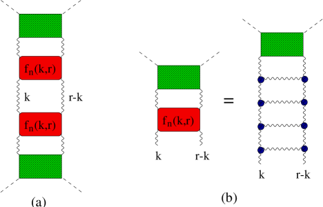
Figure 9: Diffusion in $k_{\perp}$.

Each of the upper or lower blocks in this diagram are “non-integrated gluon distribution”. The $s\rightarrow\infty$ asymptotics is governed by the rightmost singularity of the function $W(\omega,t)$ (see Eq. (51)) which is determined by the asymptotics of the coefficients $f_{n}$ at $n\rightarrow\infty$. For even $n$, these coefficients can be represented as

$$f_{2n}(t)=\int{d^{2}k\over 4\pi^{2}}{1\over\vec{k}_{\perp}^{2}(\vec{r}-\vec{k})_{\perp}^{2}}f_{n}^{A}(k_{\perp},r_{\perp})f_{n}^{B}(k_{\perp},r_{\perp}),$$ (61)

where

$$f^{A}_{n}(k_{\perp},r_{\perp})=\left({N_{c}\over 8\pi^{3}}\hat{K}_{r}\right)^{n}\!I^{A}(k_{\perp},r_{\perp}),~{}~{}~{}f^{B}_{n}(k_{\perp},r_{\perp})=\left({N_{c}\over 8\pi^{3}}\hat{K}_{r}\right)^{n}\!I^{B}(k_{\perp},r_{\perp}).$$ (62)

Let us demonstrate that the characteristic momenta $\vec{k}_{\perp}^{2}$ in the integral in Eq. (61) are $\sim m^{2}e^{\sqrt{n}}$. At large transverse momenta $k_{\perp}$ the recursion formula $f^{A}_{n+1}(k_{\perp},r_{\perp})={N_{c}\over 8\pi^{3}}\hat{K}_{r}f^{A}_{n}(k_{\perp},r_{\perp})$ can be reduced to

$$\omega\phi_{n+1}(\xi)=$$ (63)

$${g^{2}N_{c}\over 4\pi^{2}}\int d\xi^{\prime}\Bigg{[}{e^{(\xi-\xi^{\prime})/2}\over 1-e^{\xi-\xi^{\prime}}}\phi_{n}(\xi^{\prime})-\left({1\over 1-e^{\xi-\xi^{\prime}}}-{1\over\sqrt{1+4e^{2(\xi-\xi^{\prime})}}}\right)\phi_{n}(\xi)\Bigg{]}$$

where $\xi=\ln{\vec{k}_{\perp}^{2}\over m^{2}}$ and $\phi_{n}(\xi)=\left({g^{2}\over\omega}\right)^{n}{1\over|k_{\perp}|}f_{n}(\vec{k}_{\perp}^{2})$. Next, we expand the function $\phi_{n}(\xi^{\prime})$ in the integrand in Eq. (63) in Taylor series $\phi_{n}(\xi^{\prime})=\phi_{n}(\xi)+(\xi^{\prime}-\xi)\phi^{\prime}_{n}(\xi)+{1\over 2}(\xi^{\prime}-\xi)^{2}\phi"_{n}(\xi)+...$. As we shall see below, at large $n$ and $k_{\perp}$ one can neglect higher terms in Taylor expansion, and then the recursion integral equation (63) can be approximated by the differential equation

$$\omega{\partial\over\partial n}\phi(n,\xi)=(\omega_{0}-\omega)\phi(n,\xi)+c{\partial^{2}\partial\xi^{2}}\phi(n,\xi),$$ (64)

where $c={7\over\pi^{2}}g^{2}\zeta(3)$, $\zeta(3)\simeq$ 1.202. This equation describes the diffusion of the “particle” where $n$ serves as a time and $\xi$ as a coordinate. It is well known that at large time $n$ the mean position $\xi$ of the “particle” is proportional to $\sqrt{n}$, and therefore our approximation of Eq. (63) by the diffusion equation (64) is justified.

Thus, we must find the solution of the diffusion equation (64) with the “wall-type” boundary condition

$$\left.\phi(n,\xi)\right|_{\xi=\xi_{t}}=0,\qquad\xi_{t}\equiv\ln{\vec{r}_{\perp}^{2}\over m^{2}}$$ (65)

which reflects the fact that our approximation is not valid at $\vec{k}_{\perp}^{2}<\vec{r}_{\perp}^{2}$. It is easy to check that the solution of the Eq. (64) with the boundary condition (65) behaves at large $\xi\sim\sqrt{n}$ as

$$\phi(n,\xi)\sim{(\xi-\xi_{t})\over n^{3/2}}e^{\left({\omega_{0}\over\omega}-1\right)n}e^{-{\omega\over 4nc}(\xi-\xi_{t})^{2}}$$ (66)

where the coefficient of the proportionality may be determined by a more accurate analysis of the transition from the integral equation (63) to the diffusion equation (64).

Substituting the estimate (66) in the integral (61), we obtain

$$\left.\left({g^{2}\over\omega}\right)^{n}f_{n}\right|_{n\rightarrow\infty}\sim{1\over n^{3/2}}e^{\left({\omega_{0}\over\omega}-1\right)n},$$ (67)

which gives

$$W(\omega,t)\sim\sum\left({g^{2}\over\omega}\right)^{n}f_{n}=\int_{1}^{\infty}dn{1\over n^{3/2}}e^{\left({\omega_{0}\over\omega}-1\right)n}=\sqrt{\omega_{0}-\omega}.$$ (68)

We see that the singularity is located at the same point $\omega=\omega_{0}$ as in the case of forward scattering, although its character is slightly different: $\sqrt{\omega_{0}-\omega}$ instead of ${1\over\sqrt{\omega_{0}-\omega}}$.[1]

At $t=0$ there is no “wall” boundary condition (65) which shows that the diffusion equation (64) leads to $|\xi|\sim\sqrt{n}$. This means that the characteristic momenta $k_{\perp}$ are either very large, $\vec{k}_{\perp}^{2}\sim m^{2}e^{\sqrt{n}}$, or very small, $\vec{k}_{\perp}^{2}\sim m^{2}e^{-\sqrt{n}}$. The large contribution from the region of small $k_{\perp}$ region indicates the possibility of the breakdown of perturbative QCD for high-energy scattering.

We can safely apply pQCD to high-energy scattering if the characteristic transverse momenta of the gluons $k_{\perp}$ in the ladder are large. For the $\gamma^{\ast}\gamma^{\ast}$ with $p_{A}^{2}\sim p_{A}^{2}\sim m^{2}\gg\Lambda_{\rm QCD}^{2}$ one can check by explicit calculation that the characteristic $k_{\perp}$ for the first few diagrams are $\sim m$. However, due to the diffusion in $k_{\perp}$ , the leading contribution to the loop integrals comes from the gluon momenta which are either very large, $\vec{k}_{\perp}^{2}\sim m^{2}e^{\sqrt{n}}$, or very small, $\vec{k}_{\perp}^{2}\sim m^{2}e^{-\sqrt{n}}$. Due to the asymptotic freedom, the fact that the $k_{\perp}$ may be very large at $n\rightarrow\infty$ only strengthens the applicability of pQCD. On the contrary, the fact that $k_{\perp}$ may be small questions the applicability of pQCD to the high-energy $\gamma^{\ast}\gamma^{\ast}$ scattering.

To take into account the asymptotic freedom, one may consider the BFKL equation with the running coupling constant. Each of the upper or lower blocks in the diagram in Fig. 9 is a “non-integrated gluon distribution”

$$F^{A(B)}(k_{\perp},r_{\perp};s)=\sum{1\over n!}\left(g^{2}\ln{s\over m^{2}}\right)^{n}f^{A(B)}_{n}(k_{\perp},r_{\perp})$$ (69)

which satisfies the BFKL equation

$$\omega F^{A(B)}(k_{\perp},r_{\perp};\omega)=$$ (70)

$$I^{A(B)}(k_{\perp},r_{\perp})+{g^{2}\over 8\pi^{3}}N_{c}\int d^{2}k^{\prime}_{\perp}K(k_{\perp},k^{\prime}_{\perp},r_{\perp})F^{A(B)}(k^{\prime}_{\perp},r_{\perp};\omega)$$

where $F(k_{\perp},r_{\perp};\omega)$ is a Mellin transform of Eq. (69):

$$F(k_{\perp},r_{\perp};s)={1\over 2\pi i}\int d\omega\left({s\over m^{2}}\right)^{\omega}F(k_{\perp},r_{\perp};\omega).$$

In order to account for the asymptotic freedom, we can replace $g^{2}$ in the right-hand side of the Eq. (70) by $g^{2}(\vec{k}_{\perp}^{2})$:

$$\omega F(k_{\perp},r_{\perp};\omega)=I(k_{\perp},r_{\perp})+{g^{2}(k_{\perp})\over 8\pi^{3}}N_{c}\int d^{2}k^{\prime}_{\perp}K(k_{\perp},k^{\prime}_{\perp},r_{\perp})F(k^{\prime}_{\perp},r_{\perp};\omega).$$ (71)

This equation exceeds the LLA accuracy but it it can be demonstrated that in the case of large (or small) $\vec{k}_{\perp}^{2}$ the replacement $g^{2}\rightarrow g^{2}(\vec{k}_{\perp}^{2})$ agrees with the renormalization group analysis [12]). Another arguments in favor of taking into account these particular sub-leading logs follows from the analysis of the renormalon contributions.[14]

At large $k_{\perp}$ one can replace the equation (71) by the corresponding diffusion equation. It turns out that at large momentum transfer $|t|=\vec{r}_{\perp}^{2}$ the rightmost singularity of $F(k_{\perp},r_{\perp};\omega)$ is located simply at $t=12{\alpha_{s}(|t|)\over\pi}N_{c}\ln 2$. At $t=0$ the diffusion goes in both directions leading to the contributions coming from $k_{\perp}\sim\Lambda_{\rm QCD}$. If one removes these contributions “by hand” (imposing the “wall” condition at $\vec{k}_{\perp}^{2}=\Lambda_{\rm QCD}$), one obtains a discrete set of Regge poles which condense from the right to the point $\omega=0$.[12] A more satisfactory solution of the problem of the diffusion to small $k_{\perp}$ would be to match the hard pomeron with the soft Landshoff-Donnachie pomeron (responsible for the high-energy hadron-hadron scattering) which presumably comes from the high-energy exchanges by soft gluons (see, however, Ref. 15 for an alternative “hard” soft pomeron). Another possibility is that the diffusion to small $k_{\perp}$ disappears if one takes into account the unitarization effects.[16]

The proper way to address the problem of running coupling constant in the BFKL equation is to use the NLO BFKL kernel in the renormalization-group analysis.[17] The NLO correction to the anomalous dimension of the corresponding leading-twist gluon operator consists of two parts: the conformal part and the running coupling part. The conformal part (see also Ref. 18) corrects the intercept of the BFKL pomeron (57), while the running coupling part, besides replacing $12{\alpha_{s}\over\pi}N_{c}\ln 2$ by $12{\alpha_{s}(q^{2})\over\pi}N_{c}\ln 2$ in the leading order, leads to the non-Regge terms in the energy dependence of the cross section. The numerical value of the correction to the hard pomeron’s intercept introduced by the conformal part of the NLO BFKL kernel is large and negative. Its exact contribution is somewhat difficult to estimate.[19, 20] There are hopes, however, that collinear singularities causing this large NLO correction cancel each other at higher orders in $\alpha_{s}$.[21]

2.5 Reggeized gluons and unitarization of the pomeron

As I mentioned above, the bare pomeron violates the Froissart bound so we need to unitarize the BFKL pomeron. There are several approaches to the unitarization: effective reggeon field theory,[22] the generalized LLA [23] equivalent to the quantum mechanics of reggeized gluons, and the dipole model.[24, 25] We postpone the discussion of the dipole model until the next section and turn the attention to reggeon-based schemes of the unitarization.

The reggeized gluon can be defined as a “hard pomeron” for the quark-quark scattering. We have seen that the gluon propagator ${1\over\vec{k}_{\perp}^{2}}$ describing the exchange between two quarks to the left of the cut in Fig. 4 is replaced in the next order by the factor (41) coming from two diagrams in Fig. 8a,b. Thus, in the first two orders in perturbation theory the propagator describing the exchange between two quarks with gluon (color octet) quantum numbers in the $t$ channel has the form

$${1\over\vec{k}_{\perp}^{2}}\left(1-\alpha_{s}N_{c}\ln{s\over m^{2}}\int{d^{2}k^{\prime}_{\perp}\over 4\pi^{2}}{\vec{k}_{\perp}^{2}\over(\vec{k}^{\prime})_{\perp}^{2}(\vec{k}-\vec{k}^{\prime})_{\perp}^{2}}\right).$$ (72)

It can be demonstrated (either by direct summation of the Feynman diagrams [1] or by evolution of the Wilson-line operators, see Sec. 3 below), that in the LLA the logarithmic factor in parenthesis exponentiates, therefore the exchange between two quarks is described by the “reggeized” gluon propagator

$${1\over\vec{k}_{\perp}^{2}}\left({s\over m^{2}}\right)^{\alpha_{\rm reg}(\vec{k}_{\perp}^{2})},$$ (73)

where

$$\alpha_{\rm reg}(t=-\vec{k}_{\perp}^{2})=-\alpha_{s}N_{c}\int{d^{2}k^{\prime}_{\perp}\over 4\pi^{2}}{\vec{k}_{\perp}^{2}\over(\vec{k}^{\prime})_{\perp}^{2}(\vec{k}-\vec{k}^{\prime})_{\perp}^{2}}$$ (74)

is the trajectory of the reggeized gluon in the plane of complex momenta in the leading order in $\alpha_{s}$. Recently, this trajectory was computed in the next-to-leading order in $\alpha_{s}$ by direct summation of Feynman diagrams [26] and by calculation of the two-loop anomalous dimensions of the relevant Wilson-line operators.[27]

In terms of the reggeized gluons the BFKL ladder can be resummed as shown in Fig. 9 where the dash-dotted line denotes reggeized gluon (73) and the reggeon-reggeon-particle interaction is described by Lipatov’s vertex (30).

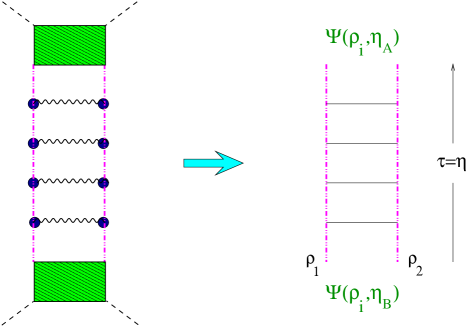
Figure 10: BFKL ladder as a propagator of the two-reggeon state. Reggeized gluons are represented by dash-dot-dot lines.

(The expansion of the reggeon trajectory in powers of $g^{2}$ reproduces the BFKL result (50) after combining the terms with like powers of $g^{2}$). This diagram can be interpreted as an evolution with respect to “time” $\equiv$ rapidity of the two-particle state described by the wave function $\Psi(\rho_{1},\rho_{2})$ in quantum mechanics with the Hamiltonian [12]

$$\hat{H}_{12} = {g^{2}N_{c}\over 16\pi^{2}}\Big{\{}\ln|\hat{p}_{1}|^{2}+\ln|\hat{p}_{2}|^{2}$$

$$+ {1\over\hat{p}_{1}|^{2}\hat{p}_{1}|^{2}}\big{(}\hat{p}_{1}^{*}\hat{p}_{2}\ln|\hat{\rho}_{12}|^{2}\big{(}\hat{p}_{1}\hat{p}_{2}^{*}+c.c.\big{)}+4C\Big{\}}$$

where $\rho_{j}=x^{(j)}_{\perp 1}+ix^{(j)}_{\perp 2}$, $\hat{p}_{j}=i{\partial\over\partial\rho_{j}}$ (index $j=1,2$ numbers the particles), and $\hat{\rho}_{12}$ is the coordinate operator ($\rho_{12}\equiv\rho_{1}-\rho_{2}$). The first two “kinetic terms” correspond to the propagators of the reggeized gluons and the third term describes the interaction of reggeized gluons by exchange potential coming from product of two Lipatov’s vertices given by Eq. (36). The Hamiltonian (2.5) has a property of holomorphic separability [28]

$$\hat{H}_{12}=\hat{h}_{12}+\hat{h}_{12}^{*},$$ (76)

where

$$\hat{h}_{12}={g^{2}N_{c}\over 16\pi^{2}}\left\{\ln\hat{p}_{1}\hat{p}_{2}+{1\over\hat{p}_{1}}(\ln\rho_{12})\hat{p}_{1}+{1\over\hat{p}_{2}}(\ln\rho_{12})\hat{p}_{2}+2C\right\},$$ (77)

and C=0.557 is Euler’s constant. The generalized LLA is the summation of the diagrams shown in Fig. 11 (see the discussion in Ref. 29).

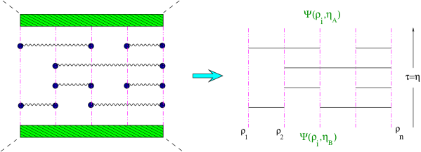
Figure 11: Generalized LLA as quantum mechanics of the reggeized gluons.

The number of reggeized gluons in $t$ channel is conserved, so the sum of the diagrams in Fig. 10a can be described by quantum mechanics of the reggeized gluons with pairwise interaction (2.5),

$$\hat{H}=\sum_{i<k}T^{a}_{i}T^{a}_{k}H_{ik},$$ (78)

where $H_{ik}$ is obtained from Eq. (2.5) by the trivial replacement $1\rightarrow i,~{}2\rightarrow k$.

The unitarity follows from the representation of the sum of these diagrams as a generalized eikonal [30] (see Fig. 12).

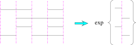
Figure 12: Quantum mechanics of the reggeized gluons as a generalized eikonal.

In the multi-color limit ($N_{c}\rightarrow\infty,~{}g^{2}N_{c}$-fixed), the non-planar diagrams vanish hence only the interaction between the adjacent reggeons survives (the unitarity still holds true). The color structure is then unique and the Hamiltonian reduces to [28]

$$\hat{H}={1\over 2}\sum_{i=1}^{n}\hat{H}_{i,i+1},$$ (79)

where ${1\over 2}$ comes from the fact that the adjacent gluons are in the octet state. Using the property of the holomorphic separability (76), it is possible to reduce the quantum mechanics of the reggeons described by the Hamiltonian (79) to the XXX Heisenberg model with spin $s=0$.[31] Unfortunately, the explicit solution for the number of the magnets $k\geq 3$ ($\equiv$ number of the reggeons) has not yet been found. For the $k=3$ (the so-called Odderon state of three reggeized gluons) the variational estimates give the intercept at the value of $J$ slightly below 1 [32, 33] (recently, another Odderon-type solution with intercept at $j=1$ was found in Ref. 34).

In synopsis, we have found the subset of the non-LLA diagrams which restores unitarity in the s-channel and in the large $N_{c}$ limit this subset reduces to the one-dimensional quantum mechanical model (XXX magnet with $s=0$).

3 Operator expansion for high-energy scattering

The expansion of the amplitudes at high energy in Wilson-line operators is very useful in a situation like small-$x$ DIS from the nucleon or nucleus. As the usual light-cone expansion provides the operator language for the DGLAP evolution, the high-energy OPE gives us the operator form of the BFKL equation. In the case of deep inelastic scattering there are two different scales of transverse momentum $k_{\perp}$, and therefore it is natural to factorize the amplitude in the product of contributions of hard and soft parts coming from the regions of small and large transverse momenta, respectively. Technically we choose the factorization scale $Q>\mu>m_{N}$, and the integrals over $\vec{k}_{\perp}^{2}>\mu^{2}$ give the coefficient functions in front of light-cone operators while the contributions from $\vec{k}_{\perp}^{2}<\mu^{2}$ give matrix elements of these operators normalized at the normalization point $\mu$. In the final result for the structure functions the dependence on $\mu$ in the coefficient functions and in the matrix elements cancels out yielding the $Q^{2}$ behavior of structure functions of DIS.

In the case of the high-energy (Regge ) limit, all the transverse momenta are of the same order of magnitude, but colliding particles strongly differ in rapidity, thus it is natural to factorize in the rapidity space. Factorization in rapidity space means that a high-energy scattering amplitude can be represented as a convolution of contributions due to “fast” and “slow” fields. To be precise, we choose a certain rapidity $\eta_{0}$ to be a “rapidity divide” and we call fields with $\eta>\eta_{0}$ fast and fields with $\eta<\eta_{0}$ slow where $\eta_{0}$ lies in the region between spectator rapidity $\eta_{A}$ and target rapidity $\eta_{B}$. (The interpretation of these fields as fast and slow is literally true only in the rest frame of the target but we will use this terminology for any frame). Similarly to the case of usual OPE, the integrals over fast fields give the coefficient functions in front of the relevant (Wilson-line) operators while the integrals over slow fields form matrix elements of the operators. For a 2$\Rightarrow$2 particle scattering in Regge limit $s\gg m^{2}$ (where $m$ is a common mass scale for all other momenta in the problem $t\sim p_{A}^{2}\sim(p^{\prime}_{A})^{2}\sim p_{B}^{2}\sim(p^{\prime}_{B})^{2}\sim m^{2}$) this operator expansion has the form [35]

$$A(p_{A},p_{B}\Rightarrow p^{\prime}_{A},p^{\prime}_{B}) = \sum\int d^{2}x_{1}...d^{2}x_{n}C^{i_{1}...i_{n}}(x_{1},...x_{n})$$ (80)

$$\times \langle p_{B}|{\rm Tr}\{U_{i_{1}}(x_{1})...U_{i_{n}}(x_{n})\}|p^{\prime}_{B}\rangle.$$

(As usual, $s=(p_{A}+p_{B})^{2}$ and $t=(p_{A}-p^{\prime}_{A})^{2}$). Here $x_{i}~{}(i=1,2)$ are the transverse coordinates (orthogonal to both $p_{A}$ and $p_{B}$) and $U_{i}(x)=U^{\dagger}(x){i\over g}{\partial\over\partial x_{i}}U(x)$ where the Wilson-line operator $U(x)$ is the gauge link ordered along the infinite straight line corresponding to the “rapidity divide” $\eta_{0}$. Both coefficient functions and matrix elements in Eq. (80) depend on the $\eta_{0}$ but this dependence is canceled in the physical amplitude just as the scale $\mu$ (separating coefficient functions and matrix elements) disappears from the final results for structure functions in case of usual factorization. Typically, we have the factors $\sim(g^{2}\ln s/m^{2}-\eta_{0})$ coming from the “fast” integral and the factors $\sim g^{2}\eta_{0}$ coming from the “slow” integral so they combine in a usual log factor $g^{2}\ln s/m^{2}$. In the leading log approximation these factors sum up into the BFKL pomeron.

Unlike usual factorization, the expansion (80) does not have the additional meaning of perturbative versus nonperturbative separation – both the coefficient functions and the matrix elements have perturbative and non-perturbative parts. This happens because the coupling constant in a scattering process is determined by the scale of transverse momenta. When we perform the usual factorization in hard ($k_{\perp}>\mu$) and soft ($k_{\perp}<\mu$) momenta, we calculate the coefficient functions perturbatively (because $\alpha_{s}(k_{\perp}>\mu)$ is small) whereas the matrix elements are non-perturbative. Conversely, when we factorize the amplitude in rapidity, both fast and slow parts have contributions coming from the regions of large and small $k_{\perp}$. In this sense, coefficient functions and matrix elements enter the expansion (80) on equal footing.

3.1 High-energy OPE vs light-cone expansion

Let me remind the idea of the usual light-cone expansion for the deep inelastic scattering (DIS) at moderate $x$. First, we take formal limit $Q^{2}\rightarrow\infty$ and expand near the light cone ($\equiv$in inverse powers of $Q^{2}$). The amplitude of DIS is then reduced to the matrix elements of the light-cone operators which are known as parton densities in the nucleon. At this step, the support lines for these operators are exactly light-like, leading to the logarithmical divergence in transverse momenta. The reason for this divergence is the following: when we expand T-product of electromagnetic currents near the light cone we assume that there are no hard quarks and gluons inside the proton. However, the matrix elements of light-cone operators contain formally unbounded integrations over $\vec{k}_{\perp}^{2}$, consequently there are hard quarks and gluons in these matrix elements. It is well known how to proceed in this case: define the renormalized light-cone operators with the integrations over the transverse momenta $\vec{k}_{\perp}^{2}>\mu^{2}$ cut off and expand the T-product of electromagnetic currents in a set of these renormalized light-cone operators rather than in a set of the original unrenormalized ones (see e.g. Ref. 36). After that, the matrix elements of these operators (parton densities) contain factors $\ln{\mu^{2}\over m^{2}}$ and the corresponding coefficient functions contain $\ln{Q^{2}\over\mu^{2}}$. When we calculate the amplitude we add these factors together, the dependence on the factorization scale $\mu$ cancels, and we get the usual DIS logarithmical factors $\ln{Q^{2}\over m^{2}}$. An advantage of this method is that the dependence of structure functions on $Q^{2}$ is determined by the dependence of matrix elements of the light-cone operators on $\mu$ which is governed by the renormalization group.

To get the operator expansion for high-energy scattering, we will proceed in the same way. At first, we take the formal Regge limit $s\rightarrow\infty$ and demonstrate that the amplitude in this limit is reduced to matrix elements of the Wilson-line operators representing the two quarks moving with the speed of light in the gluon “cloud.” Formally, we obtain the operators $U$ ordered along light-like lines. Matrix elements of such operators contain divergent longitudinal integrations reflecting the fact that light-like gauge factor corresponds to a quark moving with speed of light (i.e., with infinite energy). The reason for this divergency is the same as in the case of usual light-cone expansion: the fast-quark propagator in the gluon “cloud” is replaced by the light-like Wilson line assuming that there are no fast gluons in the cloud. However, when we calculate the matrix element of the Wilson-line operators with light-like support, the integration over the rapidities of the gluon $\eta_{p}$ is unbounded so our divergency comes from the fast part of the cloud which does not really belong there. Indeed, if the rapidity of the gluon $\eta_{p}$ is of the order of the rapidity of the quark, this gluon is a fast one. As a result, it will contribute to the coefficient function (in front of the operator constructed from the slow fields) rather than to the matrix element of the operator. Similarly to the case of DIS, we need some regularization of the Wilson-line operator which cuts off the fast gluons. As demonstrated in Ref. 35, it can be done by changing the slope of the supporting lines. If we wish the longitudinal integration stop at $\eta=\eta_{0}$, we should order our gauge factors $U$ along a line parallel to $n=\sigma p_{1}+\tilde{\sigma}p_{2}$, then the coefficient functions in front of Wilson-line operators (impact factors) will contain logarithms $\sim g^{2}\ln 1/\sigma$. Similarly to DIS, when we calculate the amplitude, we add the terms $\sim g^{2}\ln 1/\sigma$ coming from the coefficient functions to the terms $\sim g^{2}\ln{\sigma\over m^{2}/s}$ coming from matrix elements so that the dependence on the “rapidity divide” $\sigma$ cancels and we get the usual high-energy factors $g^{2}\ln{s\over m^{2}}$ which are responsible for BFKL pomeron. Again, the advantage of this method is that the energy dependence of the amplitude is determined by the renorm-group-like evolution equations for the Wilson-line operators with respect to the slope of the line.

3.2 High-energy asymptotics as a scattering from the shock-wave field.

Consider again for simplicity the high-energy $\gamma^{*}\gamma^{*}$ scattering (6). To put this amplitude in a form symmetric with respect the top and bottom photons, we make a shift of the coordinates in the currents by $(z_{\bullet},0,0_{\perp})$ and then reverse the sign of $z_{\bullet}$. This gives:

$$A(s,t) = -i{2\over s}\int d^{2}z_{\perp}dz_{\bullet}dz_{*}\int\!d^{4}xd^{4}ye^{-ip_{A}\cdot x-ip_{B}\cdot y}e^{-i\alpha_{r}z_{\bullet}+i\beta_{r}z_{\ast}-i(r,z)_{\perp}}$$ (81)

$$\times \Big{\langle}0\Big{|}T\{j_{A}(x_{\bullet},x_{*}+z_{*},x_{\perp}+z_{\perp})j^{\prime}_{A}(0,z_{*},z_{\perp})$$

$$\times j_{B}(y_{\bullet}+z_{\bullet},y_{*},y_{\perp})j^{\prime}_{B}(z_{\bullet},0,0_{\perp})\}\Big{|}0\Big{\rangle}.$$

As we discussed in Sec. 1, $\alpha_{r}\sim\beta_{r}\sim{m^{2}\over s}$ so it can be neglected.

It is convenient to start with the upper part of the diagram, i.e., to study how fast quarks move in an external gluonic field. After that, functional integration over the gluon fields will reproduce us the Feynman diagrams of the type of Fig. 3:

$$A(s,t) = -i{s\over 2}\int\!d^{2}z_{\perp}e^{-i(r,z)_{\perp}}~{}~{}{\cal N}^{-1}\int{\cal D}A\,e^{iS(A)}{\rm det}(i\nabla)$$

$$\times \left\{{2\over s}\int\!dz_{*}\int\!d^{4}x\,e^{-ip_{A}\cdot x}\left\langle Tj_{A}(x_{\bullet},x_{*}+z_{*},x_{\perp}+z_{\perp})j^{\prime}_{A}(0,z_{*},z_{\perp})\right\rangle_{A}\right\}$$

$$\times \left\{{2\over s}\int\!dz_{\bullet}\int\!d^{4}y\,e^{-ip_{B}\cdot y}\left\langle Tj_{B}(y_{\bullet}+z_{\bullet},y_{*},y_{\perp})j^{\prime}_{B}(z_{\bullet},0,0_{\perp})\right\rangle_{A}\right\},$$

where

$$\langle Tj_{\mu}(x)j_{\nu}(y)\rangle_{A}\equiv\frac{\int{\cal D}\psi{\cal D}\bar{\psi}e^{iS(\psi,A)}j_{\mu}(x)j_{\nu}(y)}{\int{\cal D}\psi{\cal D}\bar{\psi}e^{iS(\psi,A)}}.$$ (83)

Here $S(A)$ and $S(\psi,A)$ are the gluon and quark-gluon parts of the QCD action respectively, and ${\rm det}(i\nabla)$ is the determinant of Dirac operator in the external gluon field.

The Regge limit $s\rightarrow\infty$ with $p_{A}^{2}$ and $p_{B}^{2}$ fixed corresponds to the following rescaling of the virtual photon momentum:

$$p_{A}=\lambda p_{1}^{(0)}+\frac{p_{A}^{2}}{2\lambda p^{(0)}_{1}\cdot p_{2}}p_{2},$$ (84)

with $p_{B}$ fixed. This is equivalent to

$$p_{1}=\lambda p_{1}^{(0)},\ \ \ p_{2}=p_{2}^{(0)},$$ (85)

where $p^{(0)}_{1}$ and $p_{2}^{(0)}$ are fixed light-like vectors so that $\lambda$ is a large parameter associated with the center-of-mass energy ($s=2\lambda p_{1}^{(0)}\cdot p_{2}^{(0)}$). Let us study the asymptotics of high-energy $\gamma^{*}\gamma^{*}$ scattering from the fixed external field

$$\int\!dx\int\!dz\delta(z_{\bullet})e^{-ip_{A}x-i(r,z)_{\perp}}\langle T\{j_{\mu}(x+z)j_{\nu}(z)\}\rangle_{A}.$$ (86)

Instead of rescaling of the incoming photon’s momentum (84), it is convenient to boost the external field instead:

$$\int\!dxdz\delta(z_{\bullet})e^{-ip_{A}x-i(r,z)_{\perp}}\langle T\{j_{\mu}(x+z)j_{\nu}(z)\}\rangle_{A}$$ (87)

$$= \int\!dxdz\delta(z_{\circ})e^{-ip^{(0)}_{A}x-i(r,z)_{\perp}}\langle T\{j_{\mu}(x+z)j_{\nu}(z)\}\rangle_{B},$$

where $p^{(0)}_{A}=p^{(0)}_{1}+{p_{A}^{2}\over s_{0}}p_{2}$ and the boosted field $B_{\mu}$ has the form

$$B_{\circ}(x_{\circ},x_{\ast},x_{\perp}) = \lambda A_{\circ}({x_{\circ}\over\lambda},x_{\ast}\lambda,x_{\perp}),$$

$$B_{\ast}(x_{\circ},x_{\ast},x_{\perp}) = {1\over\lambda}A_{\ast}({x_{\circ}\over\lambda},x_{\ast}\lambda,x_{\perp}),$$

$$B_{\perp}(x_{\circ},x_{\ast},x_{\perp}) = A_{\perp}({x_{\circ}\over\lambda},x_{\ast}\lambda,x_{\perp}),$$ (88)

where we used the notations $x_{\circ}\equiv x^{\mu}p_{1\mu}^{(0)},~{}x_{\ast}\equiv x^{\mu}p_{2\mu}$. The field

$$A_{\mu}(x_{\circ},x_{\ast},x_{\perp})=A_{\mu}({2\over s_{0}}x_{\circ}p_{1}^{(0)}+{2\over s_{0}}x_{\ast}p_{2}+x_{\perp})$$ (89)

is the original external field in the coordinates independent of $\lambda$, therefore we may assume that the scales of $x_{\circ},x_{\ast}$ (and $x_{\perp}$) in the function (89) are $O(1)$. First, it is easy to see that at large $\lambda$ the field $B_{\mu}(x)$ does not depend on $x_{\circ}$. Moreover, in the limit of very large $\lambda$ the field $B_{\mu}$ has a form of the shock wave. It is especially clear if one writes down the field strength tensor $G_{\mu\nu}$ for the boosted field. If we assume that the field strength $F_{\mu\nu}$ for the external field $A_{\mu}$ vanishes at the infinity we get

$$G_{\circ i}(x_{\circ},x_{\ast},x_{\perp}) = \lambda F_{\circ i}({x_{\circ}\over\lambda},x_{\ast}\lambda,x_{\perp})\rightarrow\delta(x_{\ast})G_{i}(x_{\perp}),$$

$$G_{{}_{\ast}i}(x_{\circ},x_{\ast},x_{\perp}) = {1\over\lambda}F_{{}_{\ast}i}({x_{\circ}\over\lambda},x_{\ast}\lambda,x_{\perp})\rightarrow 0,$$

$$G_{\circ\ast}(x_{\circ},x_{\ast},x_{\perp}) = F_{\circ\ast}({x_{\circ}\over\lambda},x_{\ast}\lambda,x_{\perp})\rightarrow 0,$$

$$G_{ik}(x_{\circ},x_{\ast},x_{\perp}) = F_{ik}({x_{\circ}\over\lambda},x_{\ast}\lambda,x_{\perp})\rightarrow 0,$$ (90)

so the only component which survives the infinite boost is $F_{\circ\perp}$ and it exists only within the thin “wall” near $x_{\ast}=0$. In the rest of the space the field $B_{\mu}$ is a pure gauge. Let us denote by $\Omega$ the corresponding gauge matrix and by $B^{\Omega}$ the rotated gauge field which vanishes everywhere except the thin wall:

$$B^{\Omega}_{\circ}=\lim_{\lambda\rightarrow\infty}\frac{\partial^{i}}{\vec{\partial}^{2}_{\perp}}G^{\Omega}_{i\circ}(0,\lambda x_{\ast},x_{\perp})\rightarrow\delta(x_{\ast})\frac{\partial^{i}}{\vec{\partial}^{2}_{\perp}}G^{\Omega}_{i}(x_{\perp}),~{}B^{\Omega}_{\ast}=B_{\perp}=0.$$ (91)

To illustrate the method, consider at first the propagator of the scalar particle (say, the Faddeev-Popov ghost) in the shock-wave background. In Schwinger’s notations we write down formally the propagator in the external gluon field $A_{\mu}(x)$ as

$$G(x,y)=\hbox{\bf\Big{(}$\!\!$\Big{(}}x\Big{|}\frac{1}{P^{2}+i\epsilon}\Big{|}y\hbox{\bf\Big{)}$\!\!$\Big{)}}=\hbox{\bf\Big{(}$\!\!$\Big{(}}x\Big{|}\frac{1}{(p+gA)^{2}+i\epsilon}\Big{|}y\hbox{\bf\Big{)}$\!\!$\Big{)}},$$ (92)

where $\hbox{\bf($\!$(}x|y\hbox{\bf)$\!$)}=\delta^{(4)}(x-y)$,

$$\hbox{\bf($\!$(}x|p_{\mu}|y\hbox{\bf)$\!$)}=-i\frac{\partial}{\partial y^{\mu}}\delta^{(4)}(x-y),~{}~{}~{}~{}\hbox{\bf($\!$(}x|A_{\mu}|y\hbox{\bf)$\!$)}=A_{\mu}(x)\delta^{(4)}(x-y).$$ (93)

Here $|x\hbox{\bf)$\!$)}$ are the eigenstates of the coordinate operator ${\cal X}|x\hbox{\bf)$\!$)}=x|x\hbox{\bf)$\!$)}$ (normalized according to the second line in the above equation). From Eq. (93) it is also easy to see that the eigenstates of the free momentum operator $p$ are the plane waves $|p\hbox{\bf)$\!$)}=\int d^{4}x\,e^{-ip\cdot x}|x\hbox{\bf)$\!$)}$. The path-integral representation of a Green function of scalar particle in the external field has the form:

$${\hbox{\bf\Big{(}$\!\!$\Big{(}}}x\Big{|}\frac{1}{{\cal P}^{2}}\Big{|}y{\hbox{\bf\Big{)}$\!\!$\Big{)}}}=-i\int_{0}^{\infty}\!d\tau{\hbox{\bf\Big{(}$\!\!$\Big{(}}}x\Big{|}e^{i\tau{\cal P}^{2}}\Big{|}y{\hbox{\bf\Big{)}$\!\!$\Big{)}}}$$

$$= -i\int_{0}^{\infty}\!d\tau{\cal N}^{-1}\int_{x(0)=y}^{x(\tau)=x}\!{\cal D}x(t)e^{-i\int_{0}^{\tau}\!dt{\dot{x}^{2}\over 4}}Pexp\{ig\int_{0}^{\tau}\!dt(B^{\Omega}_{\mu}(x(t))\dot{x}^{\mu}(t)\},$$

where $\tau$ is Schwinger’s proper time. It is clear that all the interaction with the external field $B^{\Omega}_{\mu}$ occurs at the point of the intersection of the path of the particle with the shock wave (see Fig. 13).

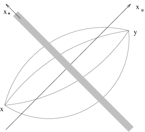
Figure 13: Propagator in the shock-wave field.

Therefore, it is convenient to rewrite at first the bare propagator

$${\hbox{\bf\Big{(}$\!\!$\Big{(}}}x\Big{|}\frac{1}{p^{2}}\Big{|}y{\hbox{\bf\Big{)}$\!\!$\Big{)}}}=\frac{i}{4\pi^{2}(x-y)^{2}}=-i\int_{0}^{\infty}\!d\tau{\cal N}^{-1}\int^{x(\tau)=x}_{x(0)=y}\!{\cal D}x(t)(\tau)e^{-i\int^{\tau}_{0}\!dt{\dot{x}^{2}\over 4}}$$ (95)

marking the point of the intersection of integration path with the plane $z_{\ast}=0$. To this end, consider the case $x_{\ast}>0,~{}y_{\ast}<0$ and insert

$$1=\int\!d\tau^{\prime}\dot{x}_{\ast}(\tau^{\prime})\delta(x_{\ast}(\tau^{\prime}))$$ (96)

in the path integral (95). (Here $\tau^{\prime}$ has the meaning of the time at which the intersection with the plane $z_{\ast}=0$ takes place). We get

$${\hbox{\bf\Big{(}$\!\!$\Big{(}}}x\Big{|}\frac{1}{p^{2}}\Big{|}y{\hbox{\bf\Big{)}$\!\!$\Big{)}}}=-i\int_{0}^{\infty}\!d\tau{\hbox{\bf\Big{(}$\!\!$\Big{(}}}x\Big{|}e^{i\tau{p^{2}}}\Big{|}y{\hbox{\bf\Big{)}$\!\!$\Big{)}}}$$

$$= -i\int_{0}^{\infty}\!d\tau\int_{0}^{\tau}\!d\tau^{\prime}{\cal N}^{-1}\int_{x(0)=y}^{x(\tau)=x}\!{\cal D}x(t)\dot{x}_{\ast}(\tau^{\prime})\delta(x_{\ast}(\tau^{\prime}))e^{-i\int_{0}^{\tau}\!dt{\dot{x}^{2}\over 4}}$$

$$= -i\int_{0}^{\infty}\!d\tau\int_{0}^{\tau}\!d\tau^{\prime}\!\int\!dz\delta(z_{*}){\cal N}^{-1}\int_{x(\tau^{\prime})=z}^{x(\tau)=x}\!\!{\cal D}x(t)\!e^{-i\int_{\tau^{\prime}}^{\tau}\!dt{\dot{x}^{2}\over 4}}{\cal N}^{-1}$$

$$\times \int_{x(0)=y}^{x(\tau^{\prime})=z}\!\!{\cal D}x(t)\dot{x}_{*}(\tau^{\prime})e^{-i\int_{0}^{\tau^{\prime}}\!dt{\dot{x}^{2}\over 4}}.$$

Making the shift of integration variable $\tau-\tau^{\prime}\rightarrow\tau$, we can rewrite the path integral (3.2) in the form:

$$-i\int_{0}^{\infty}\!d\tau\int_{0}^{\infty}\!d\tau^{\prime}\int\!dz\delta(z_{\ast})$$

$$\times {\cal N}^{-1}\int_{x(0)=z}^{x(\tau)=x}\!{\cal D}x(t)\!e^{-i\int_{0}^{\tau}\!dt{\dot{x}^{2}\over 4}}{\cal N}^{-1}\int_{x(0)=y}^{x(\tau^{\prime})=z}\!{\cal D}x(t)\dot{x}_{\ast}e^{-i\int_{0}^{\tau^{\prime}}\!dt{\dot{x}^{2}\over 4}}.$$

Using Eq. (95) and similar formula

$$\int_{0}^{\infty}\!d\tau{\cal N}^{-1}\int^{x(\tau)=x}_{x(0)=y}\!{\cal D}x(t)\dot{x}_{\mu}(\tau)e^{-i\int^{\tau}_{0}\!dt{\dot{x}^{2}\over 4}}=\frac{i(x-y)_{\mu}}{\pi^{2}(x-y)^{4}}~{}~{},$$ (99)

we arrive at the following representation of the bare propagator (in the case of $x_{\ast}>0,~{}y_{\ast}<0$):

$${\hbox{\bf\Big{(}$\!\!$\Big{(}}}x\Big{|}\frac{1}{p^{2}+i\epsilon}\Big{|}y{\hbox{\bf\Big{)}$\!\!$\Big{)}}}=\int\!dz\delta(z_{\ast})\frac{1}{4\pi^{2}(x-z)^{2}}{y_{\ast}\over\pi^{2}(z-y)^{4}}$$ (100)

where $z$ is the point of the intersection of the path of the particle with the shock wave.

Now let us recall that our particle moves in the shock-wave external field and therefore each path in the functional integral (3.2) is weighted with the additional gauge factor $Pe^{ig\int B_{\mu}dx_{\mu}}$. Since the external field exists only within the infinitely thin wall at $x_{\ast}=0$ we can replace the gauge factor along the actual path $x_{\mu}(t)$ by the gauge factor along the straight-line path shown in Fig. 13. It intersects the plane $z_{\ast}=0$ at the same point $(z_{\circ},z_{\perp})$ at which the original path does. Since the shock-wave field outside the wall vanishes we may formally extend the limits of this segment to infinity and write the corresponding gauge factor as $U^{\Omega}(z_{\perp})=[\infty p_{1}+z_{\perp},-\infty p_{1}+z_{\perp}]$. The error brought by replacement of the original path $inside$ the wall by the segment of straight line parallel to $p_{1}$ is $\sqrt{m^{2}\over s}$. Indeed, the time of the transition of the particle through the wall is proportional to the thickness of the wall which is $\sim{m^{2}\over s}$. It indicates that the particle can deviate in the perpendicular directions inside the wall only to the distances $\sqrt{m^{2}\over s}$. Thus, if the particle intersects this wall at some point $(z_{\ast},z_{\perp})$ the gauge factor $Pe^{ig\int B^{\Omega}_{\mu}dx_{\mu}}$ reduces to $U^{\Omega}(z_{\perp})$. One can now repeat for the path integral (3.2) the steps which lead us from path-integral representation of bare propagator (95) to the formula (100); the only difference will be the factor $U^{\Omega}(z_{\perp})$ in the point of the intersection of the path with the plane $z_{\ast}=0$:

$${\hbox{\bf\Big{(}$\!\!$\Big{(}}}x\Big{|}\frac{1}{{\cal P}^{2}}\Big{|}y{\hbox{\bf\Big{)}$\!\!$\Big{)}}}=\int\!dz\delta(z_{\ast})\frac{1}{4\pi^{2}(x-z)^{2}}U^{\Omega}(z_{\perp})\frac{y_{\ast}}{\pi^{2}(z-y)^{4}}$$ (101)

(in the region $x_{\ast}>0,y_{\ast}<0$). It is easy to see that the propagator in the region $x_{\ast}<0,y_{\ast}>0$ differs from Eq. (101) by the replacement $U^{\Omega}\leftrightarrow U^{\Omega\dagger}$. Also, the propagator outside the shock-wave wall (at $x_{\ast},y_{\ast}<0$ or $x_{\ast},y_{\ast}>0$) coincides with the bare propagator. The final answer for the Green function of the scalar particle in the $B^{\Omega}$ background can be written down as:

$${\hbox{\bf\Big{(}$\!\!$\Big{(}}}x\Big{|}\frac{1}{{\cal P}^{2}}\Big{|}y{\hbox{\bf\Big{)}$\!\!$\Big{)}}} = i\frac{1}{4\pi^{2}(x-y)^{2}}\theta(x_{\ast}y_{\ast})+\int\!dz\delta(z_{\ast})\frac{1}{4\pi^{2}(x-z)^{2}}$$

$$\times \{U^{\Omega}(z_{\perp})\theta(x_{\ast})\theta(-y_{\ast})-U^{\Omega\dagger}(z_{\perp})\theta(y_{\ast})\theta(-x_{\ast})\}\frac{y_{\ast}}{\pi^{2}(z-y)^{4}}.$$

We see that the propagator in the shock-wave background is a convolution of the free propagation up to the plane $z_{\ast}=0$, instantaneous interaction with the shock wave described by the Wilson-line operator $U^{\Omega}$ ($U^{\dagger\Omega}$), and another free propagation from $z$ to the final point (see Fig. 13) One can check that the Green function (3.2) is continuous as $x_{\ast}\rightarrow 0$ (or $y_{\ast}\rightarrow 0$).

In order to get the propagator in the original field $B_{\mu}$ we must perform back the gauge rotation with the $\Omega$ matrix. It is convenient to represent the result in the following form:

$${\hbox{\bf\Big{(}$\!\!$\Big{(}}}x\Big{|}{1\over{\cal P}^{2}}\Big{|}y{\hbox{\bf\Big{)}$\!\!$\Big{)}}}\!\!\!\! = \!\!\!\!\frac{i}{4\pi^{2}(x-y)^{2}}[x,y]\theta(x_{\ast}y_{\ast})+\!\!\int\!dz\delta(z_{\ast})\frac{1}{4\pi^{2}(x-z)^{2}}\!\!\!\!\!$$

$$\times \!\!\!\!\!\!\!\{U(z_{\perp};x,y)\theta(x_{\ast})\theta(-y_{\ast})-U^{\dagger}(z_{\perp};x,y)\theta(y_{\ast})\theta(-x_{\ast})\}\frac{y_{\ast}}{\pi^{2}(z-y)^{4}},$$

where

$$U(z_{\perp};x,y)=[x,z_{x}][z_{x},z_{y}][z_{y},y]~{},$$

$${}z_{x}\equiv({2\over s_{0}}z_{\circ}p^{(0)}_{1}+{2\over s_{0}}x_{\ast}p_{2},z_{\perp}),~{}~{}~{}~{}~{}z_{y}=z_{x}(x_{\ast}\leftrightarrow y_{\ast})$$ (104)

is a gauge factor for the contour made from segments of straight lines as shown in Fig. 14. Since the field $B_{\mu}$ outside the shock-wave wall is a pure gauge, the precise form of the contour does not matter as long as it starts at the point $x$, intersects the wall at the point $z$ in the direction collinear to $p_{2}$, and ends at the point $y$. We have chosen this contour in such a way that the gauge factor (104) is the same for the field $B_{\mu}$ and for the original field $A_{\mu}$ (see Eq. (88)).

The quark propagator in a shock-wave background can be calculated in a similar way (see Appendix 7.2),

$${\hbox{\bf\Big{(}$\!\!$\Big{(}}}x\Big{|}\frac{1}{{\not\!{\cal P}}}\Big{|}y{\hbox{\bf\Big{)}$\!\!$\Big{)}}}~{}=~{}-~{}\frac{{\not\!x}-{\not\!y}}{2\pi^{2}(x-y)^{4}}[x,y]\theta(x_{\ast}y_{\ast})~{}+~{}i\int\!dz\delta(z_{\ast})\frac{{\not\!x}-{\not\!z}}{2\pi^{2}(x-z)^{4}}$$

$$\times~{}\{U(z_{\perp};x,y)\theta(x_{\ast})\theta(-y_{\ast})-U^{\dagger}(z_{\perp};x,y)\theta(y_{\ast})\theta(-x_{\ast})\}\frac{{\not\!z}-{\not\!y}}{2\pi^{2}(z-y)^{4}}.$$ (105)

For the quark-antiquark amplitude in the shock-wave field (see Fig. 14)

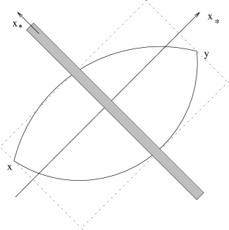
Figure 14: Quark-antiquark propagation in the shock wave.

we get

$${\rm Tr}\gamma_{\mu}{\hbox{\bf\Big{(}$\!\!$\Big{(}}}x\Big{|}\frac{1}{{\not\!{\cal P}}}\Big{|}y{\hbox{\bf\Big{)}$\!\!$\Big{)}}}\gamma_{\nu}{\hbox{\bf\Big{(}$\!\!$\Big{(}}}y\Big{|}\frac{1}{{\not\!{\cal P}}}\Big{|}x{\hbox{\bf\Big{)}$\!\!$\Big{)}}}$$ (106)

$$=~{}\frac{{\rm Tr}\gamma_{\mu}({\not\!x}-{\not\!y})\gamma_{\nu}({\not\!y}-{\not\!x})}{4\pi^{4}(x-y)^{8}}\theta(x_{\ast}y_{\ast})~{}-~{}\theta(-x_{\ast}y_{\ast})\int\!dzdz^{\prime}\delta(z_{\ast})\delta(z^{\prime}_{\ast})$$

$$\times~{}{\rm Tr}\gamma_{\mu}\frac{{\not\!x}-{\not\!z}}{2\pi^{2}(x-z)^{4}}{\not\!p}_{2}\frac{{\not\!z}-{\not\!y}}{2\pi^{2}(z-y)^{4}}\gamma_{\nu}\frac{{\not\!y}-{\not\!z}^{\prime}}{2\pi^{2}(y-z^{\prime})^{4}}{\not\!p}_{2}\frac{{\not\!z}^{\prime}-{\not\!x}}{2\pi^{2}(z^{\prime}-x)^{4}}{\rm U}(z_{\perp};z^{\prime}_{\perp}),$$

where we can write down the gauge factor U$(z_{\perp};z^{\prime}_{\perp})\equiv U(z_{\perp};x,y)U^{\dagger}(z^{\prime}_{\perp};y,x)$ as a product of two infinite Wilson-lines operators connected by gauge segments at $\pm\infty$,

$${\rm U}(z_{\perp};z^{\prime}_{\perp})$$

$$=\lim_{u\rightarrow\infty}\Big{\{}[up_{1}+z_{\perp},-up_{1}+z_{\perp}][-up_{1}+z_{\perp},-up_{1}+z^{\prime}_{\perp}][-up_{1}+z^{\prime}_{\perp},up_{1}+z^{\prime}_{\perp}]$$

$$\times[up_{1}+z^{\prime}_{\perp},up_{1}+z_{\perp}]\Big{\}}~{}=~{}U_{z}[z_{\perp},z^{\prime}_{\perp}]_{-}U^{\dagger}_{z^{\prime}}[z^{\prime}_{\perp},z_{\perp}]_{+}.$$ (107)

Here we use the notations

$$[x_{\perp},y_{\perp}]_{+}\equiv[\infty p_{1}+z_{\perp},\infty p_{1}+z^{\prime}_{\perp}],~{}~{}[x_{\perp},y_{\perp}]_{-}\equiv[-\infty p_{1}+z_{\perp},-\infty p_{1}+z^{\prime}_{\perp}].$$ (108)

As we mentioned above, the precise form of the connecting contour at infinity does not matter as long as it is outside the shock wave. We have chosen this contour in such a way that the gauge factor (107) is the same for the field $B_{\mu}$ and for the original field $A_{\mu}$ (see Eq. (88)). Now, substituting our result for quark-antiquark propagation (106) in the right-hand side of Eq. (86), one obtains

$$\int\!d^{4}x\int\!d^{4}z\,\delta(z_{\bullet})e^{-i(r,z)_{\perp}}e^{-ip_{A}\cdot x}\langle T\{j_{A}(x+z)j^{\prime}_{A}(z)\}\rangle_{A}$$ (109)

$$= \sum e_{i}^{2}\int\frac{d^{2}k_{\perp}}{4\pi^{2}}I^{A}(k_{\perp},r_{\perp}){\rm Tr}\{U(k_{\perp})U^{\dagger}(r_{\perp}-k_{\perp})\},$$

where the impact factor $I^{A}$ is given by Eq. (15). For brevity, we omit the end gauge factors (108).

Formula (107) describes a quark and antiquark moving fast through an external gluon field. After integrating over gluon fields in the functional integral we obtain the virtual photon scattering amplitude (3.2). It is convenient to rewrite it in the factorized form:

$${\cal A}(p_{A},p_{B})=i{s\over 2}\sum e_{i}^{2}\int\frac{d^{2}k_{\perp}}{4\pi^{2}}I^{A}(k_{\perp},r_{\perp})\langle\langle{\rm Tr}\{\hat{U}(k_{\perp})\hat{U}^{\dagger}(r_{\perp}-k_{\perp})\}\rangle\rangle.$$ (110)

where $I^{A}(p_{\perp})=e^{A}_{\mu}e^{A}_{\nu}I^{A}_{\mu\nu}(p_{\perp})$. The gluon fields in $U$ and $U^{\dagger}$ have been promoted to operators, a fact which we signal by replacing $U$ by $\hat{U}$, etc. The reduced matrix elements of the operator ${\rm Tr}\{\hat{U}(k_{\perp})\hat{U}^{\dagger}(r_{\perp}-k_{\perp})\}$ between the “virtual photon states” are defined as follows:

$$\langle\langle{\rm Tr}\{\hat{U}(k_{\perp})\hat{U}^{\dagger}(r_{\perp}-k_{\perp})\}\rangle\rangle = \int\!d^{2}x_{\perp}e^{-i(kx)_{\perp}}\langle\langle{\rm Tr}\{\hat{U}(x_{\perp})\hat{U}^{\dagger}(0)\}\rangle\rangle$$

$$\langle\langle{\rm Tr}\{\hat{U}(x_{\perp})\hat{U}^{\dagger}(0)\}\rangle\rangle \equiv -\int\!d^{4}z\delta(z_{\ast})e^{i(r,z)_{\perp}}\int\!d^{4}ye^{-ip_{B}\cdot y}$$

$$\quad\langle 0|T\{{\rm Tr}\{\hat{U}(x_{\perp})\hat{U}^{\dagger}(0)\}j_{B}(y+z)j^{\prime}_{B}(z)\}|0\rangle.$$

This matrix element describes the propagation of the “color dipole” in the background of the shock wave created by the second virtual photon.

It is worth noting that for a real photon our definition of the reduced matrix element can be rewritten as

$$\langle\epsilon,p_{B}|{\rm Tr}\{\hat{U}(x_{\perp})\hat{U}^{\dagger}(x^{\prime}_{\perp})\}|\epsilon^{\prime},p_{B}+\beta p_{B}\rangle~{}=~{}2\pi\delta(\beta)\,\langle\langle{\rm Tr}\{\hat{U}(x_{\perp})\hat{U}^{\dagger}(x^{\prime}_{\perp})\}\rangle\rangle,$$

where $\epsilon$ and $\epsilon^{\prime}$ represent the polarizations of the photon states. The factor $2\pi\delta(\beta)$ reflects the fact that the forward matrix element of the operator $\hat{U}(x_{\perp})\hat{U}^{\dagger}(x^{\prime}_{\perp})$ contains an unrestricted integration along $p_{1}$. Taking the integral over $\beta$ one reobtains Eq. (3.2).

3.3 Regularized Wilson-line operators

In the Regge limit (84) we have formally obtained the operators $\hat{U}$ ordered along the light-like lines. Matrix elements of such operators contain divergent longitudinal integrations which reflect the fact that light-like gauge factor corresponds to a quark moving with speed of light (i.e., with infinite energy). This divergency can be already seen at the one-loop level if one calculates the contribution to the matrix element of the two-Wilson-line operator $\hat{U}(x_{\perp})\hat{U}^{\dagger}(y_{\perp})$ between the “virtual photon states”. As I mentioned above, the reason for this divergence is that we have replaced the fast-quark propagators in the “external field” represented by two gluons coming from the bottom part of the diagram in Fig. 15a by the light-like Wilson lines in Fig. 15b.

Figure 15: A typical Feynman diagram for the $\gamma^{*}\gamma^{*}$ scattering amplitude (a) and the corresponding two-Wilson-line operator (b).

The integration over rapidities of the gluon $\eta_{p}$ in the matrix element of the light-like Wilson-line operator $\hat{U}(x_{\perp})\hat{U}^{\dagger}(y_{\perp})$ is formally unbounded , consequently we need some regularization of the Wilson-line operator which cuts off the fast gluons. As demonstrated in Ref. 35, it can be done by changing the slope of the supporting line. If we wish the longitudinal integration stop at $\eta=\eta_{0}$, we should order our gauge factors $U$ along a line parallel to $p_{\zeta}=p_{1}+\zeta p_{2}$ where $\eta_{0}=\ln\zeta$. We define

$$\hat{U}^{\zeta}(x_{\perp}) = [\infty p^{\zeta}+x_{\perp},-\infty p^{\zeta}+x_{\perp}],$$

$$\hat{U}^{\dagger\zeta}(x_{\perp}) = [-\infty p^{\zeta}+x_{\perp},\infty p^{\zeta}+x_{\perp}].$$ (112)

Matrix elements of these operators coincide with matrix elements of the operators $\hat{U}$ and $\hat{U}^{\dagger}$ calculated with the restriction $\alpha<\sigma=\sqrt{p_{A}^{2}\over s\zeta}$ imposed in the internal loops (and external tails). Let us demonstrate this using the simple example of the matrix element of the operator $\hat{U}^{\zeta}(k_{\perp})\hat{U}^{\dagger\zeta}(r_{\perp}-k_{\perp})$ coming from the diagram shown in Fig. 15. It has the form

$$\!\!\!\!\!-{i\over 2}g^{6}\int\!\frac{d\alpha_{p}}{2\pi}\frac{d^{4}p^{\prime}}{16\pi^{4}}\,\frac{[(\alpha_{p}-2\alpha^{\prime}_{k})\beta^{\prime}_{k}s-(\vec{k}+\vec{k}^{\prime})^{2}_{\perp}]\Phi^{B}(k^{\prime})}{(\zeta\alpha_{p}^{2}s+\vec{k}^{2}_{\perp}-i\epsilon)^{2}\,(\alpha^{\prime}_{k}\beta^{\prime}_{k}s-\vec{p^{\prime}}^{2}_{\perp}+i\epsilon)^{2}}$$ (113)

$$\times \frac{1}{[-(\alpha_{p}-\alpha^{\prime})(\alpha_{p}\zeta+\beta^{\prime}_{k})s-(\vec{k}-\vec{k}^{\prime})^{2}_{\perp}+i\epsilon]},$$

where the numerator comes from the product of two three-gluon vertices (18)

$${4\over s^{2}}\Gamma_{\ast\bullet}{}^{\sigma}(k,-k^{\prime})\Gamma_{\ast\bullet\sigma}(k,-k^{\prime})==(\alpha_{k}-2\alpha^{\prime}_{k})\beta^{\prime}_{k}s-(\vec{k}+\vec{k}^{\prime})^{2}_{\perp}.$$ (114)

As we shall see below, the logarithmic contribution comes from the region $\sqrt{m^{2}\over\zeta s}\gg\alpha_{k}\gg\alpha^{\prime}_{k}\sim{m^{2}\over s}$, $1\gg\beta_{p}^{\prime}\gg\beta_{p}=-\zeta\alpha_{k}\sim\sqrt{m^{2}\zeta\over s}$. In this region one can perform the integration over $\beta^{\prime}_{k}$ by taking the residue at the pole $\left[-(\alpha_{p}-\alpha^{\prime})(\alpha_{p}\zeta+\beta^{\prime}_{k})s-(\vec{k}-\vec{k}^{\prime})^{2}_{\perp}+i\epsilon\right]^{-1}$. The result is 

$$\!\!\!\!\frac{g^{6}}{s}\int\frac{d\alpha_{k}}{2\pi}\frac{d\alpha^{\prime}_{k}}{2\pi}\int\frac{d^{2}k^{\prime}_{\perp}}{4\pi^{2}}\left[\Theta(\alpha_{k}>\alpha^{\prime}_{k}>0+\Theta(0>\alpha^{\prime}_{k}>\alpha_{k})\right]$$

$$\times \frac{\left(\vec{k}^{2}_{\perp}+{p^{\prime}}_{\perp}^{2}-\alpha_{k}^{2}\zeta s/2\right)\,\Phi^{B}\left(\alpha_{k}^{\prime}p_{1}-(\alpha_{k}\zeta+{(\vec{k}-\vec{k}^{\prime})^{2}_{\perp}\over\alpha_{p}s})p_{2}+k^{\prime}_{\perp}\right)}{|\alpha_{p}-\alpha^{\prime}_{k}|\,(\zeta\alpha_{p}^{2}s+\vec{k}^{2}_{\perp}-i\epsilon)^{2}\,[\frac{\alpha^{\prime}_{k}}{\alpha_{k}}(\vec{k}-\vec{k}^{\prime})^{2}_{\perp}+\vec{p^{\prime}}^{2}_{\perp}+i\epsilon]^{2}}.$$

We see that the integral over $\alpha_{p}$ is logarithmic in the region $\sqrt{m^{2}\over\zeta s}\gg\alpha_{p}\gg\alpha^{\prime}_{k}\sim{m^{2}\over s}$ (cf. Eq. (18)). The lower limit of this logarithmical integration is provided by the matrix element itself ($\beta_{k}\sim 1$ in the lower quark bulb) while the upper limit, at $\alpha_{k}^{2}\sim m^{2}/\zeta s$ is enforced by the non-zero $\zeta$ and the result has the form

$$\langle\!\langle{\rm Tr}{\hat{U}^{\zeta}}(k_{\perp}){\hat{U}^{\dagger\zeta}}(-k_{\perp})\rangle\!\rangle_{{\rm Fig.~{}\ref{fig4}}}~{}=~{}{g^{6}\over 8\pi}\ln\left({s\over m^{2}\zeta}\right)\int\!\frac{d^{2}k^{\prime}_{\perp}}{4\pi^{2}}\frac{\vec{k}^{2}_{\perp}+{p^{\prime}}_{\perp}^{2}}{\vec{k}^{4}_{\perp}\vec{p^{\prime}}^{4}_{\perp}}I^{B}(k^{\prime}_{\perp}).$$ (116)

Similarly to the case of usual light-cone expansion, we expand the amplitude in a set of “regularized” Wilson-line operators $\hat{U}^{\zeta}$ (see Fig. 16):

$$A(p_{A},p_{B}\Rightarrow p^{\prime}_{A},p^{\prime}_{B}) = \sum\int d^{2}x_{1}...d^{2}x_{n}C(x_{1},...x_{n}:\zeta)$$

$$\times \langle p_{B}|{\rm Tr}\{\hat{U}^{\zeta}(x_{1})\hat{U}^{\dagger\zeta}(x_{2})...\hat{U}^{\zeta}(x_{n-1})\hat{U}^{\dagger\zeta}(x_{n})|p^{\prime}_{B}\rangle.$$

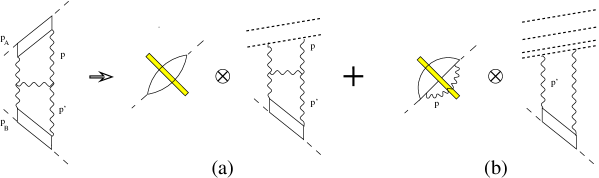
Figure 16: Decomposition into product of coefficient function and matrix element of the two-Wilson-line operator for a typical Feynman diagram. (Double Wilson line corresponds to the fast-moving gluon.)

The coefficient functions in front of Wilson-line operators (impact factors) will contain logarithms $\sim g^{2}\ln 1/\sigma$ and the matrix elements $\sim g^{2}\ln{s\sigma\over m^{2}}$. Similar to DIS, when we calculate the amplitude, we add the terms $\sim g^{2}\ln 1/\sigma$ coming from the coefficient functions (see Fig. 16b) to the terms $\sim g^{2}\ln{\sigma\over m^{2}/s}$ coming from matrix elements (see Fig. 16a) so that the dependence on the “rapidity divide” $\sigma$ cancels resulting in the usual high-energy factors $g^{2}\ln{s\over m^{2}}$ which are responsible for the BFKL pomeron, cf. (50).

In the LLA, the light-like operators $\hat{U}$ and $\hat{U}^{\dagger}$ in Eq. (110) should be replaced by the Wilson-line operators $\hat{U}^{\zeta}$ and $\hat{U}^{\dagger\zeta}$ ordered along $n\parallel p_{A}$. Indeed, let us compare the matrix element (116) shown in Fig. 6b to the corresponding physical amplitude (17) shown in Fig. 6a. The integral in Eq. (17) is similar to the one for the matrix element of the operator (116), except that there is now a factor of the upper quark bulb and the integral over $p_{\perp}$. If we calculate only the contribution of the diagram in Fig. 6a , we would get (cf. Eq. (2.2))

$$\sim i{g^{6}\over 4\pi}\ln\left({s\over m^{2}}\right)\int\!\frac{d^{2}k_{\perp}}{4\pi^{2}}\frac{d^{2}k^{\prime}_{\perp}}{4\pi^{2}}\frac{\vec{k}^{2}_{\perp}+\vec{p^{\prime}}^{2}_{\perp}}{\vec{k}^{4}_{\perp}\vec{p^{\prime}}^{4}_{\perp}}I^{A}(k_{\perp})I^{B}(k^{\prime}_{\perp})$$ (118)

which agrees with the with estimate Eq. (116), if we set $\zeta={p_{A}^{2}\over s}$. This corresponds to making the line in the path-ordered exponential collinear to the momentum of the photon.

3.4 One-loop evolution of Wilson-line operators.

As we demonstrated in previous section, with the LLA accuracy, the improved version of the factorization formula Eq. (109) has the operators $\hat{U}$ and $\hat{U}^{\dagger}$ “regularized” at $\zeta\sim{p_{A}^{2}\over s}$:

$$\int d^{4}x\int d^{4}z\,\delta(z_{\bullet})e^{-ip_{A}\cdot x-i(r,z)_{\perp}}T\{j_{A}(x+z)j^{\prime}_{A}(z)\}$$

$$= \sum_{i}e_{i}^{2}\int\frac{d^{2}k_{\perp}}{4\pi^{2}}I^{A}(k_{\perp},r_{\perp}){\rm Tr}\{\hat{U}^{\zeta={m^{2}\over s}}(k)\hat{U}^{\dagger\zeta={m^{2}\over s}}(r-k)\}.$$

In the next-to-leading order in $\alpha_{s}$ we will have the corrections
$\sim\alpha_{s}{\rm Tr}\hat{U}(x_{\perp})\hat{U}^{\dagger}(y_{\perp}){\rm Tr}\hat{U}(y_{\perp})\hat{U}^{\dagger}(z_{\perp})$, see Fig. 16.

Next we derive the equation for the evolution of these operators with respect to slope $\zeta$ (in the LLA). In order to find the behavior of the matrix elements of the operators $\hat{U}^{\zeta}(x_{\perp})\hat{U}^{\dagger\zeta}(y_{\perp})$ on the slope $\zeta$ we must take the matrix element of this operator “normalized” at $\zeta_{1}$ and integrate over the momenta with $\sigma_{1}=\sqrt{m^{2}\over s\zeta_{1}}>\alpha>\sigma_{2}=\sqrt{m^{2}\over s\zeta_{2}}$ (similar to the case of ordinary Wilson OPE where in order to find the dependence of the light-cone operator on the normalization point $\mu$ we integrate over the momenta with virtualities $\mu_{1}^{2}>p^{2}>\mu_{2}^{2}$). The result will be the operators $\hat{U}$ and $\hat{U}^{\dagger}$ “normalized” at the slope $\zeta_{2}$ times the coefficient functions determining the kernel of the evolution equation. The calculation of the kernel is essentially identical to the calculation of the impact factor with the only difference of having initial gluons instead of quarks. Here we will present only the outline of the calculations; the details can be found in Appendix C.

In the first order in $\alpha_{s}$ there are two one-loop diagrams for the matrix element of operator $\hat{U}(x_{\perp})\hat{U}^{\dagger}(y_{\perp})$ in external field (see Fig. 17).

Figure 17: One-loop diagrams for the evolution of the two-Wilson-line operator.

This external field is made from slow gluons with $\alpha<\zeta_{2}$. Like the case of the fast quark propagator considered above, it is convenient to go to the rest frame of “fast” gluons, as a consequence the “slow” gluons will form a thin pancake.

Let us start with the diagram shown in Fig. 17a. We will calculate the one-loop evolution of the operator $\hat{U}(x_{\perp})\otimes\hat{U}^{\dagger}(y_{\perp})\equiv\{\hat{U}(x_{\perp})\}^{i}_{j}\{\hat{U}^{\dagger}(y_{\perp})\}^{k}_{l}$ with the non-convoluted color indices. In the LLA, the slope $p^{\zeta}$ of the operators $U$ can be replaced by $p_{1}$. Using the expression for the axial-gauge gluon propagator in the external field (7.4)  we obtain:

$$\hat{U}(x_{\perp})\otimes\hat{U}^{\dagger}(y_{\perp})\rangle_{A}$$ (120)

$$=-ig^{2}\int du[\infty p_{1},up_{1}]_{x}t^{a}[up_{1},-\infty p_{1}]_{x}\int dv[-\infty p_{1},vp_{1}]_{y}t^{b}[vp_{1},\infty p_{1}]_{y}$$

$$\times~{}\hbox{\bf\Big{(}$\!\!$\Big{(}}up_{1}+x_{\perp}\Big{|}(p_{1\xi}-{\cal P}_{\bullet}\frac{p_{2\xi}}{p\cdot p_{2}}){\cal O}^{\xi\eta}(p_{1\eta}-\frac{p_{2\eta}}{p\cdot p_{2}}{\cal P}_{\bullet})\Big{|}vp_{1}+y_{\perp}\hbox{\bf\Big{)}$\!\!$\Big{)}}_{ab}.$$

Hereafter we use the space-saving notation

$$[un,vn]_{x}\equiv[un+x_{\perp},vn+x_{\perp}].$$ (121)

We may drop the terms proportional to ${\cal P}_{\bullet}$ in the parenthesis since they lead to the terms proportional to the integrals of total derivatives, namely

$$\int du[\infty p_{1},up_{1}]t^{a}[up_{1},-\infty p_{1}]p_{1\mu}(D^{\mu}\Phi(up_{1},...))_{ab}$$ (122)

$$= \int du\frac{d}{du}\{[\infty p_{1},up_{1}]t^{a}[up_{1},-\infty p_{1}](\Phi(up_{1},...))_{ab}\}=0$$

and similar for the total derivative with respect to $v$. Now, we can rewrite Eq. (120) in the form

$$\langle\hat{U}(x_{\perp})\otimes\hat{U}^{\dagger}(y_{\perp})\rangle_{A}~{}=~{}-ig^{2}\int du[\infty p_{1},up_{1}]_{x}t^{a}[up_{1},-\infty p_{1}]_{x}$$

$$\otimes \int dv[-\infty p_{1},vp_{1}]_{y}t^{b}[vp_{1},\infty p_{1}]_{y}\hbox{\bf\Big{(}$\!\!$\Big{(}}up_{1}+x_{\perp}\Big{|}{\cal O}_{\bullet\bullet}\Big{|}vp_{1}+y_{\perp}\hbox{\bf\Big{)}$\!\!$\Big{)}}_{ab}.$$

As in the calculation of the quark propagator, it is convenient to go to the rest frame of “fast” gluons. In this frame the “slow” gluons will form a thin pancake shown in Fig. 18. At first, we consider the case $x_{\ast}>0,~{}y_{\ast}<0$.

Figure 18: Path integrals describing one-loop diagrams for Wilson-line operators in the shock-wave field background.

It is clear from the picture that we can rewrite Eq. (3.4) as follows:

$$\langle\hat{U}(x_{\perp})\hat{U}^{\dagger}(y_{\perp})\rangle_{A} = -ig^{2}t^{a}U(x_{\perp})\otimes t^{b}U^{\dagger}(y_{\perp})$$

$$\times \int_{0}^{\infty}\!du\!\int_{-\infty}^{0}\!dv\hbox{\bf\Big{(}$\!\!$\Big{(}}up^{(0)}_{A}+x_{\perp}\Big{|}{\cal O}_{\bullet\bullet}\Big{|}vp^{(0)}_{A}+y_{\perp}\hbox{\bf\Big{)}$\!\!$\Big{)}}_{ab}$$

(we shall calculate only the contribution $\sim U$ which comes from the region $x_{\ast}>0,y_{\ast}<0$ - the term $\sim U^{\dagger}$ coming from $x_{\ast}>0,y_{\ast}<0$ is similar). Technically it is convenient to find at first the derivative of the integral of gluon propagator in the right-hand side of Eq. (3.4) with respect to $x_{\perp}$. Using the thin-wall approximation we obtain

$$\hbox{\bf\Big{(}$\!\!$\Big{(}}x\Big{|}{\cal O}_{\bullet\bullet}\Big{|}y\hbox{\bf\Big{)}$\!\!$\Big{)}} = {s^{2}\over 2}\int\!dz\delta(z_{\ast})\frac{\ln(x-z)^{2}}{16\pi^{2}x_{\ast}}$$

$$\times \{2[FF](z_{\perp})-i[DF](z_{\perp})\}\frac{1}{4\pi^{2}(z-y)^{2}},$$

where

$$\ [DF](x_{\perp}) \stackrel{{\scriptstyle\rm def}}{{\equiv}} \int du[\infty p_{1},up_{1}]_{x}D^{\alpha}F_{\alpha\bullet}(up_{1}+x_{\perp})[up_{1},-\infty p_{1}]_{x},$$

$$\ [FF](x_{\perp}) \stackrel{{\scriptstyle\rm def}}{{\equiv}} \int\!du\int\!dv\Theta(u-v)[\infty p_{1},up_{1}]_{x}F^{\xi}_{\bullet}(up_{1}+x_{\perp})$$ (126)

$$\times [up_{1},vp_{1}]_{x}F_{\xi\bullet}(vp_{1}+x_{\perp})[vp_{1},-\infty p_{1}]_{x}.$$

It is easy to see that the operators in braces are in fact the total derivatives of $U$ and $U^{\dagger}$ with respect to translations in the perpendicular directions,

$$\vec{\partial}_{\perp}^{2}U(x_{\perp}) \equiv \frac{\partial^{2}}{\partial x_{i}\partial x_{i}}U(x_{\perp})=-i[DF](x_{\perp})+2[FF](x_{\perp}),$$

$$\vec{\partial}_{\perp}^{2}U^{\dagger}(x_{\perp}) \equiv \frac{\partial^{2}}{\partial x_{i}\partial x_{i}}U^{\dagger}(x_{\perp})=i[DF](x_{\perp})+2[FF](x_{\perp}),$$ (127)

(note that $\vec{\partial}_{\perp}^{2}U=-\partial^{2}U$).

For the derivative of the gluon propagator $(x|p_{i}{\cal O}|y)$ we obtain:

$$\!\!\!\!-ig^{2}\int\!du\!\int\!dv\hbox{\bf\Big{(}$\!\!$\Big{(}}up^{(0)}_{A}+x_{\perp}\Big{|}p_{i}{\cal O}_{\bullet\bullet}\Big{|}vp^{(0)}_{A}+y_{\perp}\hbox{\bf\Big{)}$\!\!$\Big{)}}_{ab}$$

$$= {g^{2}\over 16\pi^{4}}\int\!dz_{\perp}\!\int_{0}^{\infty}\frac{du}{u}dv\int\!dz_{\bullet}$$

$$\times \frac{(x_{\perp}-z_{\perp})_{i}[\vec{\partial}^{2}_{\perp}U(z_{\perp})]_{ab}}{[u(u\zeta s-2z_{\bullet})-(\vec{x}-\vec{z})^{2}_{\perp}-i\epsilon][v(v\zeta s+2z_{\bullet})-(\vec{y}-\vec{z})^{2}_{\perp}-i\epsilon]}.$$

The integration over $z_{\bullet}$ can be performed by taking the residue; the result is

$$-i{g^{2}\over 16\pi^{3}}\int\!dz_{\perp}\int_{0}^{\infty}\frac{du}{u}dv\frac{(x_{\perp}-z_{\perp})_{i}[\vec{\partial}^{2}_{\perp}U(z_{\perp})]_{ab}}{[(\vec{x}-\vec{z})^{2}_{\perp}v+(\vec{y}-\vec{z})^{2}_{\perp}v-uv(u+v)\zeta s+i\epsilon]}.$$ (129)

This integral diverges logarithmically when $u\rightarrow 0$ — in other words when the emission of quantum gluon occurs in the vicinity of the shock wave. (Note that if we had done integration by parts, the divergence would be at $v\rightarrow 0$, therefore there is no asymmetry between $u$ and $v$). The size of the shock wave $z_{\ast}\sim m^{-1}{\sigma_{2}\over\sigma_{1}}$ (where $1/m$ is the characteristic transverse size) serves as the lower cutoff for this integration and we obtain

$$\!\!\!\!-i{g^{2}\over 16\pi^{3}}\ln{\sigma_{1}\over\sigma_{2}}\int\!dz_{\perp}\int_{0}^{1}\frac{d\alpha}{\alpha}\frac{(x_{\perp}-z_{\perp})_{i}[\vec{\partial}^{2}_{\perp}U(z_{\perp})]_{ab}}{[(\vec{x}-\vec{z})^{2}_{\perp}\bar{\alpha}+(\vec{y}-\vec{z})^{2}_{\perp}\alpha]}$$ (130)

$$= -{g^{2}\over 16\pi^{3}}\ln{\sigma_{1}\over\sigma_{2}}\hbox{\bf\Big{(}$\!\!$\Big{(}}x_{\perp}\Big{|}{p_{i}\over\vec{p}_{\perp}^{2}}(\vec{\partial}_{\perp}^{2}U){1\over\vec{p}_{\perp}^{2}}\Big{|}y_{\perp}\hbox{\bf\Big{)}$\!\!$\Big{)}}_{ab},$$

(recall that $\bar{\alpha}\equiv 1-\alpha$). Thus, the contribution of the diagram in Fig. 18a in the LLA takes the form

$$\langle\hat{U}(x_{\perp})\hat{U}^{\dagger}(y_{\perp})\rangle_{A}~{}=~{}-\left({g^{2}\over 2\pi}\ln{\sigma_{1}\over\sigma_{2}}\right)\Bigg{\{}t^{a}U(x_{\perp})\otimes t^{b}U^{\dagger}(y_{\perp})\hbox{\bf\Big{(}$\!\!$\Big{(}}x_{\perp}\Big{|}{1\over\vec{p}_{\perp}^{2}}(\vec{\partial}_{\perp}^{2}U)$$

$$\times{1\over\vec{p}_{\perp}^{2}}\Big{|}y_{\perp}\hbox{\bf\Big{)}$\!\!$\Big{)}}_{ab}+U(x_{\perp})t^{a}\otimes U^{\dagger}(y_{\perp})t^{b}\hbox{\bf\Big{(}$\!\!$\Big{(}}x_{\perp}\Big{|}{1\over\vec{p}_{\perp}^{2}}(\vec{\partial}_{\perp}^{2}U^{\dagger}){1\over\vec{p}_{\perp}^{2}}\Big{|}y_{\perp}\hbox{\bf\Big{)}$\!\!$\Big{)}}_{ab}\Bigg{\}}.$$ (131)

where we have added the term coming from $x_{\ast}<0,y_{\ast}>0$. A corresponding result for the diagram shown in Fig. 18b can be obtained by comparing the space-time picture Fig. 18b for this process with Fig. 18a,

$$\langle\hat{U^{\zeta}}(x_{\perp})\otimes\hat{U^{\dagger\zeta}}(y_{\perp})\rangle_{A} = \left({g^{2}\over 2\pi}\ln{\sigma_{1}\over\sigma_{2}}\right)U(x_{\perp})\otimes t^{a}U^{\dagger}(y_{\perp})t^{b}$$ (132)

$$\times \hbox{\bf\Big{(}$\!\!$\Big{(}}y_{\perp}\Big{|}{1\over\vec{p}_{\perp}^{2}}(\vec{\partial}^{2}U){1\over\vec{p}_{\perp}^{2}}\Big{|}y_{\perp}\hbox{\bf\Big{)}$\!\!$\Big{)}}_{ab}.$$

Likewise, the diagram in Fig. 18c yields

$$\langle\hat{U^{\zeta}}(x_{\perp})\otimes\hat{U^{\dagger\zeta}}(y_{\perp})\rangle_{A} = \left({g^{2}\over 2\pi}\ln{\sigma_{1}\over\sigma_{2}}\right)t^{a}U(x_{\perp})t^{b}\otimes U^{\dagger}(y_{\perp})$$ (133)

$$\times \hbox{\bf\Big{(}$\!\!$\Big{(}}x_{\perp}\Big{|}{1\over\vec{p}_{\perp}^{2}}(\vec{\partial}^{2}U){1\over\vec{p}_{\perp}^{2}}\Big{|}x_{\perp}\hbox{\bf\Big{)}$\!\!$\Big{)}}_{ab}.$$

The total result for the one-loop evolution of two-Wilson-line operator is the sum of Eqs. (131), (132), and (133),

$$\langle\{\hat{U}^{\zeta_{1}}(x_{\perp})\}^{i}_{j}\{\hat{U}^{\dagger\zeta_{1}}(y_{\perp})\}^{k}_{l}\rangle_{A}={g^{2}\over 8\pi^{3}}\ln{\sigma_{1}\over\sigma_{2}}\int dz_{\perp}$$ (134)

$$\times~{}\left\{-\left[\{\hat{U}^{\dagger\zeta_{2}}(z_{\perp})\hat{U}^{\zeta_{2}}(x_{\perp})\}^{k}_{j}\{\hat{U}^{\zeta_{2}}(z_{\perp})\hat{U}^{\dagger\zeta_{2}}(y_{\perp})\}^{i}_{l}\right.\right.$$

$$+~{}\{\hat{U}^{\zeta_{2}}(x_{\perp})\hat{U}^{\dagger\zeta_{2}}(z_{\perp})\}^{i}_{l}\{\hat{U}^{\dagger\zeta_{2}}(y_{\perp})\hat{U}^{\zeta_{2}}(z_{\perp})\}^{k}_{j}$$

$$-~{}\left.\delta^{k}_{j}\{\hat{U}^{\zeta_{2}}(x_{\perp})\hat{U}^{\dagger\zeta_{2}}(y_{\perp})\}^{i}_{l}-\delta^{i}_{l}\{\hat{U}^{\dagger\zeta_{2}}(y_{\perp})\hat{U}^{\zeta_{2}}(x_{\perp})\}^{k}_{j}\right]\frac{(\vec{x}-\vec{z},\vec{y}-\vec{z})_{\perp}}{(\vec{x}-\vec{z})^{2}_{\perp}(\vec{y}-\vec{z})^{2}_{\perp}}$$

$$+~{}\left[\{\hat{U}^{\zeta_{2}}(z_{\perp})\}^{i}_{j}{\rm Tr}\{\hat{U}^{\zeta_{2}}(x_{\perp})\hat{U}^{\dagger\zeta_{2}}(z_{\perp})\}-N_{c}\{\hat{U}^{\zeta_{2}}(x_{\perp})\}^{i}_{j}\right]\{\hat{U}^{\dagger\zeta_{2}}(y_{\perp})^{k}_{l}\}$$

$$\times~{}\frac{1}{(\vec{x}-\vec{z})^{2}_{\perp}}~{}+~{}\{\hat{U}^{\zeta_{2}}(x_{\perp})\}^{i}_{j}\left[\{\hat{U}^{\dagger\zeta_{2}}(z_{\perp})\}^{k}_{l}{\rm Tr}\{\hat{U}^{\zeta_{2}}(z_{\perp})\hat{U}^{\dagger\zeta_{2}}(y_{\perp})\}\right.$$

$$-~{}\left.\left.N_{c}\{\hat{U}^{\dagger\zeta_{2}}(y_{\perp})\}^{k}_{l}\right]\frac{1}{(\vec{y}-\vec{z})^{2}_{\perp}}\right\}.$$

The evolution of a general $n$-Wilson-line operator is presented in Appendix 7.3.

3.5 BFKL pomeron from the evolution of the Wilson-line operators

As we demonstrated in Sec. 3.2, with the LLA accuracy the improved version of the factorization formula Eq. (109) has the operators $U$ and $U^{\dagger}$ “regularized” at $\zeta\sim{p_{A}^{2}\over s}$:

$$\!\!\!\!\int d^{4}x\int d^{4}z\,\delta(z_{\bullet})e^{-ip_{A}\cdot x-i(r,z)_{\perp}}T\{j_{A}(x+z)j^{\prime}_{A}(z)\}\qquad$$

$$= \sum_{i}e_{i}^{2}\int\frac{d^{2}k_{\perp}}{4\pi^{2}}I^{A}(k_{\perp},r_{\perp}){\rm Tr}\{U^{\zeta={m^{2}\over s}}(k)U^{\dagger\zeta={m^{2}\over s}}(r-k)\}+O(g^{2}).$$

In the next-to-leading order in $\alpha_{s}$ we will have the corrections
$\sim\alpha_{s}{\rm Tr}U(x_{\perp})U^{\dagger}(y_{\perp}){\rm Tr}U(y_{\perp})U^{\dagger}(z_{\perp})$, see Fig. 16. The matrix element of this operator $\langle\!\langle U^{\zeta}(x_{\perp})U^{\dagger\zeta}(y_{\perp})\rangle\!\rangle$ (see Eq. (3.2) for the definition) describes the gluon-photon scattering at large energies $\sim s$. (Hereafter we will wipe the label $(\hat{})$ from the notation of the operators). The behavior of this matrix element with energy is determined by the dependence on the “normalization point” $\zeta$. From the one-loop results for the evolution of the operators $U$ and $U^{\dagger}$ (134) it is easy to obtain the following evolution equation:[35, 37]

$$\zeta\frac{\partial}{\partial\zeta}{\cal U}(x_{\perp},y_{\perp}) = -{\alpha_{s}N_{c}\over 4\pi^{2}}\!\int\!dz_{\perp}\Big{\{}{\cal U}(x_{\perp},z_{\perp})+{\cal U}(z_{\perp},y_{\perp})-{\cal U}(x_{\perp},y_{\perp})$$ (136)

$$+ {\cal U}(x,z){\cal U}(z,y)\Big{\}}\frac{(\vec{x}-\vec{y})_{\perp}^{2}}{(\vec{x}_{\perp}-\vec{z}_{\perp})^{2}(\vec{z}_{\perp}-\vec{y}_{\perp})^{2}},$$

where

$${\cal U}(x_{\perp},y_{\perp})\equiv\frac{1}{N_{c}}({\rm Tr}\{U(x_{\perp})[x_{\perp},y_{\perp}]_{-}U^{\dagger}(y_{\perp})[y_{\perp},x_{\perp}]_{+}\}-N_{c})$$ (137)

(cf. Eq. (107)). Note that right-hand side of this equation is both infrared (IR) and ultraviolet (UV) finite. We see that as a result of the evolution, the two-line operator ${\rm Tr}\{UU^{\dagger}\}$ is the same operator (times the kernel) plus the four-line operator ${\rm Tr}\{UU^{\dagger}\}{\rm Tr}\{UU^{\dagger}\}$. The result of the evolution of the four-line operator will be the same operator times some kernel plus the six-line operator of the type ${\rm Tr}\{UU^{\dagger}\}{\rm Tr}\{UU^{\dagger}\}{\rm Tr}\{UU^{\dagger}\}+{\rm Tr}\{UU^{\dagger}UU^{\dagger}\}{\rm Tr}\{UU^{\dagger}\}$ and so on. Therefore it is instructive to consider at first the linearization of the Eq. (136) with the number of operators $U$ conserved during the evolution.

The linear evolution of the two-line operator ${\cal U}(x_{\perp},y_{\perp})$ is governed by the BFKL equation 

$$\!\!\!\!\zeta\frac{\partial}{\partial\zeta}{\cal U}(x_{\perp},y_{\perp})$$ (139)

$$\!\!\!\!=-{\alpha_{s}\over 4\pi^{2}}N_{c}\int\!dz_{\perp}\left\{{\cal U}(x_{\perp},z_{\perp})+{\cal U}(z_{\perp},y_{\perp})-{\cal U}(x_{\perp},y_{\perp})\right\}{(\vec{x}-\vec{y})_{\perp}^{2}\over(\vec{x}-\vec{z})_{\perp}^{2}(\vec{z}-\vec{y})_{\perp}^{2}}.$$

Let us start from the simplest case of forward matrix elements (which describes, for example, the small-x DIS from the virtual photon). Then the equation (139) takes the form

$$\zeta\frac{\partial}{\partial\zeta}\langle\!\langle{\cal U}(x_{\perp})\rangle\!\rangle=-{\alpha_{s}\over 4\pi^{2}}N_{c}\int\!dz_{\perp}[{\cal U}(x-z_{\perp})+{\cal U}(z_{\perp})-{\cal U}(x_{\perp})]{\vec{x}_{\perp}^{2}\over(\vec{x}-\vec{z})_{\perp}^{2}\vec{z}_{\perp}^{2}},$$ (140)

where $\langle\!\langle{\cal U}(x_{\perp})\rangle\!\rangle\equiv\langle\!\langle{\cal U}(x_{\perp},0)\rangle\!\rangle$ (see Eq. (3.2)). The eigenfunctions of this equation are powers $(x_{\perp}^{2})^{-{1\over 2}+i\nu}$ and the eigenvalues are $-{\alpha_{s}\over\pi}N_{c}\chi(\nu)$, where $\chi(\nu)=-{\rm Re}\psi({1\over 2}+i\nu)-C$. Therefore, the evolution of the operator ${\cal U}$ takes the form:

$$\langle\!\langle{\cal U}^{\zeta_{1}}(x_{\perp})\rangle\!\rangle = \int\!\frac{d\nu}{2\pi^{2}}(\vec{x}_{\perp}^{2})^{{1\over 2}+i\nu}\left(\frac{\zeta_{1}}{\zeta_{2}}\right)^{-{\alpha_{s}\over\pi}N_{c}\chi(\nu)}$$ (141)

$$\times \int\!dz_{\perp}(\vec{z}_{\perp}^{2})^{-{3\over 2}-i\nu}\langle\!\langle{\cal U}^{\zeta_{2}}(z)\rangle\!\rangle$$

We may proceed with this evolution as long as the upper limit of our logarithmic integrals over $\alpha$, $\sqrt{p_{A}^{2}\over\zeta s}$, is much larger than the lower limit ${p_{B}^{2}\over s}$ determined by the lower quark bulb, see the discussion in Sec. 3.3. It is convenient to stop evolution at a certain point $\zeta_{0}$ such as

$$\zeta_{0}=\sigma^{2}{s\over m^{2}},~{}~{}~{}\sigma\ll 1,~{}~{}~{}~{}g^{2}\ln\sigma\ll 1,$$ (142)

then the relative energy between the Wilson-line operator ${\cal U}^{\zeta_{0}}$ and lower virtual photon will be $s_{0}=m^{2}\sigma^{2}$ which is big enough to apply our usual high-energy approximations (such as pure gluon exchange and substitution $g_{\mu\nu}\rightarrow{2\over s_{0}}p_{2\mu}p_{1\nu}$) but small in a sense that one does not need take into account the difference between $g^{2}\ln{s\over m^{2}}$ and $g^{2}\ln{s\over m^{2}\sigma^{2}}$. Finally, the evolution (139) takes the form:

$$\langle\!\langle{\cal U}^{\zeta={m^{2}\over s}}(x_{\perp})\rangle\!\rangle=\!\int\!\frac{d\nu}{2\pi^{2}}(x_{\perp}^{2})^{{1\over 2}+i\nu}(\frac{s}{m^{2}})^{{2\alpha_{s}\over\pi}N_{c}\chi(\nu)}\!\int\!dz_{\perp}(z_{\perp}^{2})^{-{3\over 2}-i\nu}\langle\!\langle{\cal U}^{\zeta_{0}}(z_{\perp})\rangle\!\rangle.$$ (143)

Now let us rewrite this evolution in terms of original operators $UU^{\dagger}$ in the momentum representation. One obtains:

$$\langle\!\langle{\rm Tr}\{U^{\zeta={m^{2}\over s}}(p_{\perp})U^{\dagger\zeta={m^{2}\over s}}(-p_{\perp})\}\rangle\!\rangle~{}=~{}\int\!\frac{d\nu}{2\pi^{2}}(\vec{p}_{\perp}^{2})^{-{3\over 2}-i\nu}$$ (144)

$$~{}~{}~{}~{}~{}~{}~{}~{}~{}~{}\times\Big{(}\frac{s}{m^{2}}\Big{)}^{{2\alpha_{s}\over\pi}N_{c}\chi(\nu)}\int\!dp^{\prime}_{\perp}(\vec{p^{\prime}}_{\perp}^{2})^{{1\over 2}+i\nu}\langle\!\langle{\rm Tr}\{U^{\zeta_{0}}(p^{\prime}_{\perp})U^{\dagger\zeta_{0}}(-p^{\prime}_{\perp})\}\rangle\!\rangle$$

where we omit the gauge links at infinity (108) for brevity. Since we neglect the logarithmic corrections $\sim g^{2}\ln\sigma$ the matrix element of our operator $U^{\zeta_{0}}U^{\dagger\zeta_{0}}$ coincides with impact factor $I^{B}$ up to $O(g^{2})$ corrections:

$$\langle\!\langle{\rm Tr}\{U^{\zeta_{0}}(p_{\perp})U^{\dagger\zeta_{0}}(-p_{\perp})\}\rangle\!\rangle$$

$$= g^{4}{N_{c}^{2}-1\over 2}\sum e_{i}^{2}\int\frac{d\alpha}{\pi s}\frac{\Phi^{B}(\alpha_{p}p_{1}-\zeta_{0}\alpha_{p}p_{2}+p_{\perp})}{(\zeta_{0}\alpha_{p}^{2}+\vec{p}_{\perp}^{2})^{2}}$$

$$= g^{4}{N_{c}^{2}-1\over 2}\sum e_{i}^{2}\left({1\over\vec{p}_{\perp}^{4}}I^{B}(p_{\perp})-\delta(p_{\perp})\int dp^{\prime}_{\perp}{1\over\vec{p^{\prime}}_{\perp}^{4}}I^{B}(p^{\prime}_{\perp})\right).$$

Combining Eqs. (110), (144), and (3.5) we reproduce the leading logarithmic result for virtual $\gamma\gamma$ scattering (59).

In the case of small-x DIS from the nucleon the matrix element of the operator $UU^{\dagger}$ describes the propagation of the “color dipole”[57] in the nucleon. The evolution of the matrix element $\mbox{$\langle N|$}{\cal U}\mbox{$|N\rangle$}$ is the same as Eq. (144) with the only difference that the lower impact factor $I^{B}$ should be substituted by the nucleon impact factor $I^{N}$ determined by the matrix element of the operator $UU^{\dagger}$ between the nucleon states:

$$\langle N,p_{B}|{\rm Tr}\{U^{\zeta_{0}}(x_{\perp})U^{\dagger\zeta_{0}}(0)\}|N,p_{B}+\beta p_{2}\rangle=2\pi\delta(\beta)\int\!\frac{dp_{\perp}}{4\pi^{2}}e^{i(px)_{\perp}}{1\over\vec{p}_{\perp}^{4}}I^{N}(p_{\perp})$$ (146)

where $2\pi\delta(\beta)$ reflects the fact that matrix element of the operator $UU^{\dagger}$ contains unrestricted integration along $p^{\zeta_{0}}$, (cf. Eq. (3.2)). The nucleon impact factor $I^{B}(p_{\perp})$ defined in (146) is a phenomenological low-energy characteristic of the nucleon. In the BFKL evolution it plays a role similar to that of a nucleon structure function at low normalization point for DGLAP evolution. In principle, it can be estimated using QCD sum rules or phenomenological models of nucleon.

In conclusion, let us present the results for the linear evolution for the non-forward case. Due to the conformal invariance of the tree-level QCD the eigenfunctions of the equation (139) are powers [12]

$$\left({(\vec{x}-\vec{y})_{\perp}^{2}\over(\vec{x}-\vec{x}_{0})_{\perp}^{2}(\vec{y}-\vec{x}_{0})_{\perp}^{2}}\right)^{{1\over 2}+i\nu}$$ (147)

where $x_{0}$ is arbitrary. The eigenvalues are the same as for the forward case, $-{\alpha_{s}\over\pi}N_{c}\chi(\nu)$. The corresponding formula for the result of the evolution of the two-Wilson-line operator has the form:

$${\cal U}^{\zeta_{1}}(x_{\perp},y_{\perp}) = \int d\nu d^{2}x_{0}{\nu^{2}\over\pi^{4}}\left({(\vec{x}-\vec{y})_{\perp}^{2}\over(\vec{x}-\vec{x}_{0})_{\perp}^{2}(\vec{y}-\vec{x}_{0})_{\perp}^{2}}\right)^{{1\over 2}-i\nu}$$ (148)

$$\times \left({\zeta_{1}\over\zeta_{2}}\right)^{-{\alpha_{s}\over\pi}N_{c}\chi(\nu))}{\cal U}^{\zeta_{2}}(x_{0},\nu)$$

where

$${\cal U}^{\zeta}(x,\nu)~{}\equiv~{}\int dx^{\prime}\int dy^{\prime}{1\over(\vec{x}^{\prime}-\vec{y}^{\prime})_{\perp}^{4}}\left({(x^{\prime}-y^{\prime})^{2}\over(\vec{x}^{\prime}-\vec{x})_{\perp}^{2}(\vec{y}^{\prime}-\vec{x})_{\perp}^{2}}\right)^{{1\over 2}+i\nu}{\cal U}^{\zeta}(x^{\prime}_{\perp},y^{\prime}_{\perp})$$ (149)

It is worth noting that at large momentum transfers $-t=\vec{r}_{\perp}^{2}\gg m_{N}^{2}$ the nucleon impact factor is determined by the well-studied electric and magnetic form factors of the nucleon

$$I_{N}(k_{\perp},r_{\perp})\stackrel{{\scriptstyle\vec{k}_{\perp}^{2}\gg m^{2}}}{{=}}\delta_{\lambda\lambda^{\prime}}F_{1}^{p+n}(t)+{1\over 2ms}\bar{u}(p^{\prime},\lambda^{\prime})\not\!p_{1}\!\not\!r_{\perp}u(p,\lambda)F_{2}^{p+n}(t),$$ (150)

which gives an opportunity to calculate the amplitude of deeply virtual Compton scattering from the nucleon at small $x$ without any model assumptions.[40]

3.6 Non-linear evolution of Wilson lines

Unlike the linear evolution, the general picture is very complicated: not only the number of operators $U$ and $U^{\dagger}$ increase after each evolution but they form increasingly complicated structures like those displayed in Eq. (152) below. In the leading log approximation the evolution of the $2n$-line operators such as ${\rm Tr}\{UU^{\dagger}\}{\rm Tr}\{UU^{\dagger}\}...{\rm Tr}\{UU^{\dagger}\}$ comes from either self-interaction diagrams or from the pair-interactions ones (see Fig. 19)

Figure 19: Typical diagrams for the one-loop evolution of the $n$-line operator.

The one-loop evolution equations for these operators can be constructed using the pair-wise kernels calculated in the Appendix C. For instance, the evolution equation for the four-line operator appearing in the right-hand side of Eq. (136) has the form:

$$\zeta\frac{\partial}{\partial\zeta}{\rm Tr}\{U_{x}[x,z]_{-}U^{\dagger}_{z}[z,x]_{+}\}{\rm Tr}\{U_{z}[z,y]_{-}U^{\dagger}_{y}[y,z]_{+}\}$$

$$= -{g^{2}\over 16\pi^{3}}\int\!dt_{\perp}\Bigg{\{}\Big{[}{\rm Tr}\{U_{x}[x,t]_{-}U^{\dagger}_{t}[t,x]_{+}\}{\rm Tr}\{U_{t}[t,z]_{-}U^{\dagger}_{z}[z,t]_{+}\}$$

$$- N_{c}{\rm Tr}\{U_{x}[x,z]_{-}U^{\dagger}_{z}[z,x]_{+}\}\Big{]}{\rm Tr}\{U_{z}[z,y]_{-}U^{\dagger}_{y}[y,z]_{+}\}\frac{(\vec{x}-\vec{z})_{\perp}^{2}}{(\vec{x}-\vec{t})_{\perp}^{2}(\vec{z}-\vec{t})_{\perp}^{2}}$$

$$+ {\rm Tr}\{U_{x}[x,z]_{-}U^{\dagger}_{z}[z,x]_{+}\}\frac{(\vec{y}-\vec{z})_{\perp}^{2}}{(y-t)_{\perp}^{2}(\vec{z}-\vec{t})_{\perp}^{2}}$$

$$\times \Big{[}{\rm Tr}\{U_{z}[z,t]_{-}U^{\dagger}_{t}[t,z]_{+}\}{\rm Tr}\{U_{t}[t,y]_{-}U^{\dagger}_{y}[y,t]_{+}\}$$

$$- N_{c}{\rm Tr}\{U_{z}[z,y]_{-}U^{\dagger}_{y}[y,z]_{+}\}\Big{]}$$

$$+ \Big{[}{\rm Tr}\{U_{x}[x,z]_{-}U^{\dagger}_{z}[z,t]_{+}U_{t}[t,y]_{-}U^{\dagger}_{y}[y,z]_{+}U_{z}[z,y]_{-}U^{\dagger}_{t}[t,x]_{+}\}$$

$$+ {\rm Tr}\{U_{x}[x,t]_{-}U^{\dagger}_{t}[t,z]_{+}U_{z}[z,y]_{-}U^{\dagger}_{y}[y,t]_{+}U_{t}[t,z]_{-}U^{\dagger}_{z}[z,x]_{+}\}$$

$$- 2{\rm Tr}\{U_{x}[x,y]_{-}U^{\dagger}_{y}\}[y,x]_{+}\Big{]}$$

$$\times \left[-\frac{(\vec{x}-\vec{t},\vec{y}-\vec{t})_{\perp}}{(\vec{x}-\vec{t})_{\perp}^{2}(y-t)_{\perp}^{2}}-\frac{1}{(\vec{z}-\vec{t})_{\perp}^{2}}\right.$$

$$+ \left.\frac{(\vec{x}-\vec{t},\vec{z}-\vec{t})_{\perp}}{(\vec{x}-\vec{t})_{\perp}^{2}(\vec{z}-\vec{t})_{\perp}^{2}}+\frac{(\vec{z}-\vec{t},\vec{y}-\vec{t})_{\perp}}{(\vec{z}-\vec{t})_{\perp}^{2}(\vec{y}-\vec{t})_{\perp}^{2}}\right]\Bigg{\}},$$

where we have displayed the end gauge links (297) explicitly. Note that each of the separate contributions (7.3) and (299) corresponding to the diagrams in Fig. 39a and 39b diverges at large $t$ while the total result (3.6) is convergent. This is the usual cancellation of the IR divergent contributions between the emission of the real (Fig. 39a) and virtual (Fig. 39b) gluons from the colorless object (corresponding to the l.h.s. of Eq. (3.6)) (cf Eq. (136)).

Thus, the result of the evolution of the operator in the right-hand side of Eq. (3.4) has a generic form:

$${\rm Tr}\{U^{\zeta}_{x}[x,y]_{-}U^{\dagger\zeta}_{y}[y,x]_{+}\}\Rightarrow\sum_{n=0}^{\infty}(\alpha_{s}\ln\frac{\zeta}{\zeta_{0}})^{n}\int dz^{1}dz^{2}...dz^{n}$$ (152)

$$\times \Big{[}A_{n}(x,z^{1},z^{2},...z^{n},y){\rm Tr}\{U^{\zeta_{0}}_{x}[x,1]_{-}U^{\dagger\zeta_{0}}_{1}[1,x]_{+}\}$$

$$\times {\rm Tr}\{U^{\zeta_{0}}_{1}[1,2]_{-}U^{\dagger\zeta_{0}}_{2}[2,1]_{+}\}\dots{\rm Tr}\{U^{\zeta_{0}}_{n}[n,y]_{-}U^{\dagger\zeta_{0}}_{y}[y,n]_{+}\}$$

$$+ B_{n}(x,z^{1},z^{2},...z^{n},y)$$

$$\times {\rm Tr}\{U^{\zeta_{0}}_{x}[x,1]_{-}U^{\dagger\zeta_{0}}_{1}[1,2]_{+}U^{\zeta_{0}}_{2}[2,3]_{-}U^{\dagger\zeta_{0}}_{3}[3,1]_{+}U^{\zeta_{0}}_{1}[1,2]_{-}U^{\dagger\zeta_{0}}_{2}[2,x]_{+}\}$$

$$\times {\rm Tr}\{U^{\zeta_{0}}_{3}[3,4]_{-}U^{\dagger\zeta_{0}}_{4}[4,3]_{+}\}...{\rm Tr}\{U^{\zeta_{0}}_{n}[n,y]_{-}U^{\dagger\zeta_{0}}_{y}[y,n]_{+}\}+...$$

$$+ N_{c}^{n}C_{n}(x,z^{1},z^{2},...z^{n},y;){\rm Tr}\{U^{\zeta_{0}}_{x}[x,y]_{-}U^{\dagger\zeta_{0}}_{y}[y,x]_{+}\}\Big{]},$$

where $U^{(\dagger)}_{n}\equiv U^{(\dagger)}(z^{n}_{\perp})$, $[i,j]\equiv[x_{i},x_{j}]$ and
$A_{n}(x,z^{1},z^{2},\ldots,z^{n},y)$, $B_{n}(x,z^{1},z^{2},\ldots,z^{n},y)$, $\ldots$, $C_{n}(x,z^{1},z^{2},\ldots,z^{n},y)$ are the meromorphic functions that can be obtained by using the Eqs.(7.3,299) $n$ times which give us a sort of Feynman rules for calculation of these coefficient functions. If we now evolve our operators from $\zeta\sim{p_{A}^{2}\over s}$ to $\zeta_{0}$ given by Eq. (142) we shall obtain a series (152) of matrix elements of the operators $(U)^{n}(U^{\dagger})^{n}$ normalized at $\zeta_{0}$. These matrix elements correspond to small energy $\sim m^{2}$ and they can be calculated either perturbatively (in the case the “virtual photon” matrix element ) or using some model calculations such as QCD sum rules in the case of nucleon matrix element corresponding to small-$x$ $\gamma^{\ast}p$ DIS . It should be mentioned that in the case of virtual photon scattering considered above we can calculate the matrix elements of operators $UU^{\dagger}...UU^{\dagger}$ perturbatively. Because $U=1+ig\int\!A_{\mu}dx_{\mu}+...$, in the leading order in $\alpha_{s}$ we can replace by 1 all but two $U(U^{\dagger})$’s, so we return to the BFKL picture describing the evolution of the two operators $UU^{\dagger}$. The non-linear equation (136) enters the game in the situation like small-x DIS from a nucleon or nucleus when the matrix elements of the operators $UU^{\dagger}...UU^{\dagger}$ are non-perturbative, consequently there is no reason to expect that extra $U$ and $U^{\dagger}$ will lead to extra smallness. In this case, at the low “normalization point” $\zeta_{0}$ one must take into account the whole series of the operators in the right-hand side of Eq. (152), indicating the need for all the coefficients $a_{n},b_{n}...c_{n}$. Recently, these coefficients were calculated by Y. Kovchegov [37] for the case of DIS from the large nuclei in the McLerran-Venugopalan model, and the results indicate that the non-linear equation (136) leads to unitarization of the pomeron in this case.[37]

The zoo of different Wilson-line operators (152) may be reduceded by using the dipole picture.[24, 25] Technically, it arises when in each order in $\alpha_{s}\ln(\frac{\zeta}{\zeta_{0}})$ we keep only the term ${\rm Tr}\{U^{\zeta_{0}}_{x}U^{\dagger\zeta_{0}}_{1}\}{\rm Tr}\{U^{\zeta_{0}}_{1}U^{\dagger\zeta_{0}}_{2}\}...{\rm Tr}\{U^{\zeta_{0}}_{n}U^{\dagger\zeta_{0}}_{y}\}$-subtractions  in right-hand side of Eq. (152); for example, in Eq. (3.6) we keep the two first terms and disregard the third one. In other words, we take into account only those diagrams in Fig. 39 which connect the Wilson lines belonging to the same ${\rm Tr}\{U_{k}U^{\dagger}_{k+1}\}$. (This corresponds to the virtual photon wave function in the large-$N_{c}$ approximation). The diagrams of the corresponding effective theory are obtained by multiple iteration of Eq. (136) and give a picture where each “dipole” ${\rm Tr}\{U_{k}U^{\dagger}_{k+1}\}$ can create two dipoles according to Eq. (136). The motivation of this approximation is given in Refs. 24, 25, and the discussion of unitarization of the BFKL pomeron in the dipole picture is presented in Ref. 41.

3.7 Operator expansion for diffractive high-energy scattering

The nonlinear term in the equation (136) describes the triple vertex of hard pomerons in QCD. In order to see that, it is convenient to consider some process which is dominated by the three-pomeron vertex — the best example is the diffractive dissociation of the virtual photon.

The relevant operator expansion for diffractive scattering is obtained by direct generalization of our approach to the diffractive processes.[42] The total cross section for diffractive scattering has the form:

$$\sigma^{\rm diff}_{\rm tot}=\int dxe^{iqx}\int{d^{3}p^{\prime}\over(2\pi)^{3}}\sum_{X}\langle p|j_{\mu}(x)|p^{\prime}+X\rangle\langle p^{\prime}+X|j_{\nu}(0)|p\rangle,$$ (153)

$p$ and $p^{\prime}$ are the nucleon momenta and $\sum_{X}$ means the summation over all the intermediate states. We can formally write down this cross section as a “diffractive matrix element” (cf. Ref. 43):

$$\sigma^{\rm diff}_{\rm tot} = W^{\rm diff}_{\mu\nu}\stackrel{{\scriptstyle\rm def}}{{\equiv}}\int dxe^{iqx}\langle p|T\{j^{-}_{\mu}(x)j^{+}_{\nu}(0)\}|p\rangle,$$ (154)

where 

$$\!\!\!\!\langle p|T\{j^{-}_{\mu}j^{+}_{\nu}e^{i\int dz({\cal L}^{+}(z)-{\cal L}^{-}(z))}\}|p\rangle$$

$$\stackrel{{\scriptstyle\rm def}}{{\equiv}} \int{d^{3}p^{\prime}\over(2\pi)^{3}}\sum_{X}\langle p|\tilde{T}\{j_{\mu}(x)e^{-i\int dz{\cal L}(z)}\}|p^{\prime}+X\rangle$$

$$\times \langle p^{\prime}+X|T\{j_{\nu}(0)e^{i\int dz{\cal L}(z)}\}|p\rangle.$$

The superscript “–” marks the fields to the left of the cut and $+$ to the right. The definition of the T-product of the fields with $\pm$ labels is as follows: the $+$ fields are time-ordered, the $-$ fields stand in inverse time order (since they correspond to the complex conjugate amplitude), and $-$ fields stand always to the left of the $+$ ones. Therefore, the diagram technique with the double set of fields is the following: contraction of two $+$ fields is the usual Feynman propagator ${\not\!p\over p^{2}+i\epsilon}$ (for the quark field), contraction of two $-$ fields is the complex conjugated propagator ${\not\!p\over p^{2}-i\epsilon}$, and the contraction of the $-$ field with the $+$ one is the “cut propagator” $2\pi\delta(p^{2})\theta(p_{0})\not\!p$. This diagram technique for calculating T-products of double set of fields exactly reproduces the Cutkosky rules for calculation of cross sections. The light-cone expansion of the diffractive matrix element (154) gives operator definition of the diffractive parton distributions.[44]

Let us discuss the high-energy operator expansion for the diffractive amplitude $W^{\rm diff}_{\mu\nu}$. Similarly to the case of usual amplitude (110), we get in the lowest order in $\alpha_{s}$

$$W^{\rm diff} = \sum_{{\rm flavors}}\!e_{i}^{2}\int{d^{2}k_{\perp}\over 4\pi^{2}}I^{A}(k_{\perp},0)$$ (157)

$$\times \langle N|{\rm Tr}\{W^{\zeta=m^{2}/s}(k_{\perp})W^{\dagger,\zeta=m^{2}/s}(-k_{\perp})\}|N\rangle,$$

where $W(k_{\perp})$ is a Fourier transform of

$$W(x_{\perp})=V^{\dagger}(x_{\perp})U(x_{\perp}),~{}~{}~{}W^{\dagger}(x_{\perp})=U^{\dagger}(x_{\perp})V(x_{\perp}).$$ (158)

Here $U(x_{\perp})$ denotes the Wilson-line operator constructed from $+$ fields and $V(x_{\perp})$ denotes the same operator constructed from $-$ fields:

$$U^{\zeta}(x_{\perp})=[\infty p_{1}+x_{\perp},-\infty p_{1}+x_{\perp}]^{+},~{}~{}~{}V(x_{\perp})=[\infty e+x_{\perp},-\infty e+x_{\perp}]^{-}.$$ (159)

After integration over fast quarks, the slope of the Wilson lines is $\zeta=x_{B}\equiv{Q^{2}\over s}$, see the discussion in Sec. 3.3.

The evolution equation (with respect to the slope of the supporting line) turns out to have the same form as Eq. (136) for non-diffractive amplitudes:

$$\zeta\frac{d}{d\zeta}{\cal W}(x_{\perp},y_{\perp})=-{\alpha_{s}N_{c}\over 4\pi^{2}}\int dz_{\perp}{(\vec{x}-\vec{y})_{\perp}^{2}\over(\vec{x}-\vec{z})_{\perp}^{2}(\vec{z}-\vec{y})_{\perp}^{2}}$$

$$\times \Big{\{}{\cal W}(x_{\perp},z_{\perp})+{\cal W}(x_{\perp},z_{\perp})-{\cal W}(x_{\perp},y_{\perp})+{\cal W}(x_{\perp},z_{\perp}){\cal W}(z_{\perp},y_{\perp})\Big{\}},$$

where

$${\cal W}(x_{\perp},y_{\perp})\stackrel{{\scriptstyle\rm def}}{{\equiv}}{1\over N_{c}}{\rm Tr}\{W(x_{\perp})W^{\dagger}(y_{\perp})\}~{}-~{}1,$$ (161)

(cf. Eq. (137). Similarly, the linear evolution is:

$$\langle N|{\cal W}^{\zeta_{1}}(x_{\perp},0)|N\rangle = \int\!\frac{d\nu}{2\pi^{2}}(\vec{x}_{\perp}^{2})^{{1\over 2}+i\nu}\left(\frac{\zeta_{1}}{\zeta_{2}}\right)^{-{3\over 2}\omega(\nu)}$$

$$\times \int\!dz_{\perp}(\vec{z}_{\perp}^{2})^{-{1\over 2}-i\nu}\langle N|{\cal W}^{\zeta_{2}}(z_{\perp},0)|N\rangle,$$

where $\omega(\nu)=2{\alpha_{s}\over\pi}N_{c}\chi(\nu)$, see Eq. (56). Let us now describe the diffractive amplitude in LLA and in leading order in $N_{c}$. In this approximation we must take into account the non-linearity in the Eq. (3.7) only once, the rest of the evolution is linear. The result is (roughly speaking) the three two-gluon BFKL ladders which couple in a certain point, see Fig. 20.

Figure 20: Amplitude of diffractive scattering in the LLA-$N_{c}$ approximation.

For the case of diffractive DIS, this evolution has the form (cf. Ref. 45):

$$\!\!\!\!\langle N|\int dy_{\perp}{\cal W}^{\zeta=x_{B}}(x_{\perp}+y_{\perp},y_{\perp})|N\rangle$$

$$= {\alpha_{s}N_{c}\over 8\pi^{3}}\int d\nu d\nu_{1}dx_{1}d\nu_{2}dx_{2}(\vec{x}_{\perp}^{2})^{{1\over 2}+i\nu}\left((\vec{x}_{1}-\vec{x}_{2})_{\perp}^{2}\right)^{-{1\over 2}+i(\nu_{1}+\nu_{2}-\nu)}$$

$$\times {\nu_{1}^{2}\nu_{2}^{2}\over\pi^{8}}\Theta(\nu;\nu_{1},\nu_{2})\int{d^{2}p^{\prime}_{\perp}\over 4\pi^{2}}\int^{s}_{Q^{2}}{dM^{2}\over M^{2}}\left({s\over M^{2}}\right)^{\omega(\nu)}\left({M^{2}\over Q^{2}}\right)^{\omega(\nu_{1})+\omega(\nu_{2})}$$

$$\times \langle p|{\cal U}^{\zeta_{0}}(x_{1},\nu_{1})|p^{\prime}\rangle\langle p^{\prime}|{\cal U}^{\zeta_{0}}(x_{2},\nu_{2})|p\rangle,$$

where $M^{2}$ is the invariant mass of the produced particles, and

$$\Theta(\nu;\nu_{1},\nu_{2}) = {\Gamma({1\over 2}-i(\nu+\nu_{1}-\nu_{2}))\Gamma({1\over 2}-i(\nu-\nu_{1}+\nu_{2}))\over\Gamma({1\over 2}+i(\nu+\nu_{1}-\nu_{2}))\Gamma({1\over 2}+i(\nu-\nu_{1}+\nu_{2}))}$$ (164)

$$\times {\Gamma^{2}({1\over 2}+i\nu)\over\Gamma^{2}({1\over 2}+i\nu)}\Omega({1\over 2}+i\nu,{1\over 2}-i\nu_{1},{1\over 2}-i\nu_{2})$$

is a certain numerical function of three conformal weights (the explicit form was found in Ref. 46 ) which has a maximum $\Theta(0,0,0)=2\pi^{7}{}_{4}F_{3}({1\over 2}){}_{6}F_{5}({1\over 2})\simeq 7766.679$ . The value of $M^{2}$ determines the rapidity gap: from $\eta=\ln{s\over Q^{2}}$ to $\eta=\ln{M^{4}\over Q^{2}s}$ we have a production of particles described by the cut part of the ladder in Fig. 20 which brings in the factor $\left({s/M^{2}}\right)^{\omega(\nu)}$ while from $\eta=\ln{M^{4}\over Q^{2}s}$ to $\eta=\ln x_{B}$ we have a rapidity gap so there are two independent BFKL ladders which bring in the factors $\left({M^{2}/Q^{2}}\right)^{\omega(\nu_{1})}$ and $\left({M^{2}/Q^{2}}\right)^{\omega(\nu_{2})}$. Since the intercept of the BFKL pomeron $\omega_{0}>0$, this cross section increases with the growth of the rapidity gap.

The coupling of BFKL ladder with non-zero momentum transfer to a nucleon is described by the matrix element $\langle p^{\prime}|{\cal U}(x,\nu)|p\rangle$. As we discussed in the previous section, at large momentum transfer it can be approximated by the electromagnetic form factor of the nucleon,

$${\cal U}(x,\nu) = \int dx^{\prime}dy^{\prime}\left({(\vec{x}^{\prime}-\vec{y}^{\prime})_{\perp}^{2}\over(\vec{x}^{\prime}-\vec{x})_{\perp}^{2}(\vec{y}^{\prime}-\vec{x})_{\perp}^{2}}\right)^{{1\over 2}+i\nu}{1\over(\vec{x}^{\prime}-\vec{y}^{\prime})_{\perp}^{4}}$$

$$\times \int{dk_{\perp}\over 4\pi^{2}}{dr_{\perp}\over 4\pi^{2}}e^{i(\vec{k},\vec{x})_{\perp}+i(\vec{r}-\vec{k},\vec{y})_{\perp}}\Big{(}\delta_{\lambda\lambda^{\prime}}F_{1}^{p+n}(-{\vec{r}}_{\perp}^{2})$$

$$+ {1\over 2ms}\bar{u}(p^{\prime},\lambda^{\prime})\not\!p_{1}\!\not\!r_{\perp}u(p,\lambda)F_{2}^{p+n}(-{\vec{r}}_{\perp}^{2})\Big{)}.$$

If one interpolates the form factors by the dipole formulas, the diffractive amplitude in the LLA-$N_{c}$ approximation (3.7) can be calculated numerically.

The non-linar equation (3.7) can be applied to the diffractive DIS from the nuclei. In this case there is an additional large parameter, the atomic number $A$, and therefore one should take into account the multitude of the non-linear vertices rather than one vertex as in Fig. 20. These “fan” diagrams were summed up in Ref. 47 resulting in a cross section which has a maximum at a certain rapidity gap (unlike the LLA-$N_{c}$ model for the nucleon where the cross section increases with the rapidity).

4 Factorization and effective action for high-energy scattering

4.1 Factorization formula for high-energy scattering

Unlike usual factorization, the coefficient functions and matrix elements enter the expansion (80) on equal footing. We could have integrated first over slow fields (having the rapidities close to that of $p_{B}$) and the expansion would have the form:

$$A(s,t)=\sum\int d^{2}x_{1}...d^{2}x_{n}D^{i_{1}...i_{n}}(x_{1},...x_{n})\langle p_{A}|{\rm Tr}\{U_{i_{1}}(x_{1})...U_{i_{n}}(x_{n})\}|p^{\prime}_{A}\rangle.$$ (166)

In this case, the coefficient functions $D$ are the results of integration over slow fields ant the matrix elements of the $U$ operators contain only the large rapidities $\eta>\eta_{0}$. The symmetry between Eqs. (1) and (2) calls for a factorization formula which would have this symmetry between slow and fast fields in explicit form.

I will demonstrate that one can combine the operator expansions (80) and (166) in the following way:[48]

$$A(s,t) = \sum{i^{n}\over n!}\int d^{2}x_{1}...d^{2}x_{n}$$

$$\times \langle p_{A}|U^{a_{1}i_{1}}(x_{1})...U^{a_{n}i_{n}}(x_{n})|p^{\prime}_{A}\rangle\langle p_{B}|U^{a_{1}}_{i_{1}}(x_{1})...U^{a_{n}}_{i_{n}}(x_{n})|p^{\prime}_{B}\rangle,$$

where $U^{a}_{i}\equiv{\mathop{\rm Tr}}(\lambda^{a}U_{i})$ ($\lambda^{a}$ are the Gell-Mann matrices). It is possible to rewrite this factorization formula in a more visual form if we agree that operators $U$ act only on states $B$ and $B^{\prime}$ and introduce the notation $V_{i}$ for the same operator as $U_{i}$ only acting on the $A$ and $A^{\prime}$ states:

$$A(s,t)=\langle p_{A}|\langle p_{B}|\exp\left(i\!\int\!d^{2}xV^{ai}(x)U^{a}_{i}(x)\right)|p^{\prime}_{A}\rangle|p^{\prime}_{B}\rangle.$$ (168)

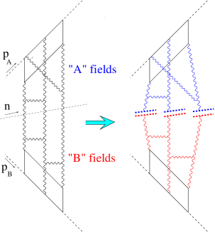
Figure 21: Structure of the factorization formula. The vector $n$ gives the direction of the “rapidity divide” between fast and slow fields.

The supporting lines of both $U$ and $V$ operators are collinear to the vector $n$ corresponding to the “rapidity divide” $\eta_{0}$. The explicit form of this vector is $n=\sigma p_{1}+\tilde{\sigma}p_{2}$, where $\tilde{\sigma}={m^{2}\over s\sigma}$ and $\ln\sigma/\tilde{\sigma}=\eta$. In a sense, formula (168) amounts to writing the coefficient functions in Eq. (80) (or Eq. (166)) as matrix elements of Wilson-line operators. Eq. (168) illustrated in Fig. 21 is our main tool for factorizing in rapidity space.

In order to understand how this expansion can be generated by the factorization formula of Eq. (168) type we have to rederive the operator expansion in axial gauge $A_{\bullet}=0$ with an additional condition $\left.A_{*}\right|_{x_{*}=-\infty}=0$ (the existence of such a gauge was illustrated in Ref. 49 by an explicit construction). It is important to note that with with power accuracy (up to corrections $\sim\sigma$) our gauge condition may be replaced by $n^{\mu}A_{\mu}=0$. In this gauge the coefficient functions are given by Feynman diagrams in the external field

$$B_{i}(x)=U_{i}(x_{\perp})\Theta(x_{*}),\qquad\qquad B_{\bullet}=B_{*}=0,$$ (169)

which is a gauge rotation of our shock wave (it is easy to see that the only nonzero component of the field strength tensor $F_{\bullet i}(x)=U_{i}(x_{\perp})\delta(x_{*})$ corresponds to shock wave). The Green functions in external field (169) can be obtained from a generating functional with a source responsible for this external field. Normally, the source for given external field $\bar{{\cal A}}_{\mu}$ is just $J_{\nu}=\bar{D}^{\mu}\bar{F}_{\mu\nu}$, so in our case the only non-vanishing contribution is $J_{*}(B)=\bar{D}^{i}\bar{F}_{i*}$. However, we have a problem because the field which we try to create by this source does not decrease at infinity. To illustrate the problem, suppose that we use another light-like gauge ${\cal A}_{*}=0$ for a calculation of the propagators in the external field (169). In this case, the only would-be nonzero contribution to the source term in the functional integral $\bar{D}^{i}\bar{F}_{i_{\bullet}}{\cal A}_{*}$ vanishes, and it looks like we do not need a source at all to generate the field $B_{\mu}$! (This is of course wrong since $B_{\mu}$ is not a classical solution). What it really means is that the source in this case lies entirely at the infinity. Indeed, when we are trying to make an external field $\bar{{\cal A}}$ in the functional integral by the source $J_{\mu}$ we need to make a shift ${\cal A}_{\mu}\rightarrow{\cal A}_{\mu}+\bar{{\cal A}}_{\mu}$ in the functional integral

$$\int{\cal D}{\cal A}\exp\left\{iS({\cal A})-i\!\int\!d^{4}xJ^{a}_{\mu}(x){\cal A}^{a\mu}(x)\right\},$$ (170)

after which the linear term $\bar{D}^{\mu}\bar{F}_{\mu\nu}{\cal A}^{\nu}$ cancels out with our source term $J_{\mu}{\cal A}^{\mu}$ and the quadratic terms lead to the Green functions in the external field $\bar{\cal A}$. (Note that the classical action $S(\bar{{\cal A}})$ for our external field $\bar{{\cal A}}=B$ (169) vanishes). However, in order to reduce the linear term $\int d^{4}x\bar{F}^{\mu\nu}\bar{D}_{\mu}{\cal A}_{\nu}$ in the functional integral to the form $\int d^{4}x\bar{D}^{\mu}\bar{F}_{\mu\nu}{\cal A}^{\nu}(x)$ we need to perform an integration by parts, and if the external field does not decrease there will be additional surface terms at infinity. In our case we are trying to make the external field $\bar{{\cal A}}=B$, consequently the linear term which need to be canceled by the source is

$${2\over s}\int\!dx_{\bullet}dx_{*}d^{2}x_{\perp}\bar{F}_{i\bullet}\bar{D}_{*}{\cal A}^{i}=\left.\int\!dx_{*}d^{2}x_{\perp}\bar{F}_{i\bullet}{\cal A}^{i}\right|^{x_{\bullet}=\infty}_{x_{\bullet}=-\infty}.$$ (171)

This contribution comes entirely from the boundaries of integration. If we recall that in our case $\bar{F}_{\bullet i}(x)=U_{i}(x_{\perp})\delta(x_{*})$ we can finally rewrite the linear term as

$$\int\!d^{2}x_{\perp}U_{i}(x_{\perp})\{{\cal A}^{i}(-\infty p_{2}+x_{\perp})-{\cal A}^{i}(\infty p_{2}+x_{\perp})\}.$$ (172)

The source term which we must add to the exponent in the functional integral to cancel the linear term after the shift is given by Eq. (172) with the minus sign. Thus, Feynman diagrams in the external field (169) in the light-like gauge ${\cal A}_{*}=0$ are generated by the functional integral

$$\!\int\!{\cal D}{\cal A}\exp\Big{\{}iS({\cal A})+i\!\int\!d^{2}x_{\perp}U^{ai}(x_{\perp})[{\cal A}^{a}_{i}(\infty p_{2}+x_{\perp})-{\cal A}^{ai}(-\infty p_{2}+x_{\perp})]\Big{\}}.$$ (173)

In an arbitrary gauge the source term in the exponent in Eq. (173) can be rewritten in the form

$$2i\int d^{2}x_{\perp}{\mathop{\rm Tr}}\{U^{i}(x_{\perp})\int^{\infty}_{-\infty}dv[-\infty p_{2},vp_{2}]_{x_{\perp}}F_{*i}(vp_{2}+x_{\perp})[vp_{2},-\infty p_{2}]_{x_{\perp}}\}.$$ (174)

Therefore, we have found the generating functional for our Feynman diagrams in the external field (169).

It is instructive to see how the source (174) creates the field (169) in perturbation theory. To this end, we must calculate the field

$$\bar{\cal A}_{\mu}(x) = \!\int\!{\cal D}{\cal A}{\cal A}_{\mu}(x)\exp\Big{\{}iS({\cal A})+2i\!\int d^{2}x_{\perp}{\mathop{\rm Tr}}\{U^{i}(x_{\perp})$$ (175)

$$\times \int^{\infty}_{-\infty}dv[-\infty p_{2},vp_{2}]_{x_{\perp}}F_{*i}(vp_{2}+x_{\perp})[vp_{2},-\infty p_{2}]_{x_{\perp}}\}\Big{\}}$$

by expansion of both $S({\cal A})$ and gauge links in the source term (174) in powers of $g$ (see Fig. 22).

Figure 22: Perturbative diagrams for the classical field (169).

In the first order one gets

$$\bar{\cal A}^{(0)}_{\mu}(x)=i\int^{\infty}_{-\infty}dv\int dz_{\perp}U^{ia}(z_{\perp})\langle{\cal A}_{\mu}(x)F^{a}_{*i}(vp_{2}+z_{\perp})\rangle,$$ (176)

where $\langle{\cal O}\rangle\equiv\int\!{\cal D}{\cal A}e^{iS_{0}}{\cal O}$. Now we must choose a proper gauge for our calculation. We are trying to create a field (169) perturbatively and therefore the gauge for our perturbative calculation must be compatible with the form (169), otherwise, we will end up with the gauge rotation of the field $B(x)$. (For example, in Feynman gauge we will get the field $\bar{\cal A}_{\mu}$ of the form of the shock wave $\bar{\cal A}_{i}=\bar{\cal A}_{\ast}=0,~{}\bar{\cal A}_{\bullet}\sim\delta(x_{\ast})$). It is convenient to choose the temporal gauge ${\cal A}_{0}=0$  with the boundary condition $\left.{\cal A}\right|_{t=-\infty}=0$ where

$${\cal A}_{\mu}(t,\vec{x})=\int^{t}_{-\infty}dt^{\prime}F_{0\mu}(t^{\prime},\vec{x}).$$ (177)

In this gauge we obtain

$$\bar{\cal A}^{(0)}_{\mu}(x)~{}=~{}\int\!{dp\over(2\pi)^{3}}\left(g_{\mu\nu}-2{p_{\mu}(p_{1}+p_{2})_{\nu}+(\mu\leftrightarrow\nu)\over s(\alpha+\beta+i\epsilon)}+{4p_{\mu}p_{\nu}\over s(\alpha+\beta+i\epsilon)^{2}}\right)$$

$$\times~{}{1\over\alpha\beta s-\vec{p}_{\perp}^{2}+i\epsilon}\int dz_{\perp}e^{-i\alpha x_{\bullet}-i\beta x_{\ast}+i\vec{p}_{\perp}(\vec{x}-\vec{z})_{\perp}}p_{2\nu}\delta(\alpha{s\over 2})\partial_{j}U^{ja}(z_{\perp})$$ (178)

where $\delta(\alpha{s\over 2})$ comes from the $\int dve^{iv\alpha{s\over 2}}$. (Note that the form of the singularity ${1\over(p_{0}+i\epsilon)}$ which follows from Eq. (177) differs from the conventional prescription $V.p.{1\over p_{0}}$). Recalling that in terms of Sudakov variables $dp={s\over 2}d\alpha d\beta dp_{\perp}$ one easily gets $\bar{\cal A}^{(0)}_{\ast}=\bar{\cal A}^{(0)}_{\bullet}=0$ and

$$\bar{\cal A}^{(0)}_{i}(x)=\theta(x_{\ast})\int\!{dp\over(2\pi)^{2}}{1\over\vec{p}_{\perp}^{2}}\int dz_{\perp}e^{i\vec{p}_{\perp}(\vec{x}-\vec{z})_{\perp}}\partial_{i}\partial_{j}U^{ja}(z_{\perp}),$$ (179)

or more formally,

$$\bar{\cal A}^{(0)}_{i}(x) = -\theta(x_{\ast}){1\over\vec{\partial}_{\perp}^{2}}\partial_{i}\partial_{j}U^{j}(x_{\perp})$$ (180)

$$= U_{i}(x_{\perp})\theta(x_{\ast})-\theta(x_{\ast}){1\over\vec{\partial}_{\perp}^{2}}(\vec{\partial}_{\perp}^{2}g_{ij}+\partial_{i}\partial_{j})U^{j}(x_{\perp}),$$

(in our notations $\vec{\partial}_{\perp}^{2}\equiv-\partial_{i}\partial^{i}$). Now, since $U_{i}(x)$ is a pure gauge field (with respect to transverse coordinates) we have $\partial_{i}U_{j}-\partial_{j}U_{i}=i[U_{i},U_{j}]$, so

$$\bar{\cal A}^{(0)}_{i}(x)=U_{i}(x_{\perp})\theta(x_{\ast})-\theta(x_{\ast})ig{\partial^{j}\over\vec{\partial}_{\perp}^{2}}[U_{i},U_{j}])(x_{\perp}).$$ (181)

Consequently, we have reproduced the field (169) up to the correction of of $g$. We will demonstrate now that this $O(g)$ correction is canceled by the next-to-leading term in the expansion of the exponent of the source term in Eq. (175). In the next-to-leading order one gets (see Fig. 22b)

$$\bar{\cal A}^{(1)}_{\mu}(x) = g\int\!dy\int\!dz_{\perp}dz^{\prime}_{\perp}U^{ja}(z_{\perp})U^{kb}(z^{\prime}_{\perp})$$

$$\times \Big{\langle}{\cal A}_{\mu}(x)2{\rm Tr}\{\partial^{\alpha}{\cal A}^{\beta}(y)[{\cal A}_{\alpha}(y),{\cal A}_{\beta}(y)]\}$$

$$\times \int\!dvF^{a}_{*j}(vp_{2}+z_{\perp})\int\!dv^{\prime}F^{b}_{*k}(vp_{2}+z^{\prime}_{\perp})\Big{\rangle}.$$

It is easy to see that $\bar{\cal A}^{(1)}_{\ast}=\bar{\cal A}^{(1)}_{\bullet}=0$ and

$$\bar{\cal A}^{(1)}_{i}(x) = -g\int\!dy\int{dp\over(2\pi)^{4}i}e^{-ip(x-y)}{1\over p^{2}}$$

$$\times \left(\partial^{k}[{\cal A}^{(0)}_{i}(y),{\cal A}^{(0)}_{k}(y)]+[{\cal A}^{(0)k}(y),\partial_{i}{\cal A}^{(0)}_{k}(y)-(i\leftrightarrow k)]\right).$$

Since ${\cal A}^{(0)}_{k}$ is given by Eq. (181), this reduces to

$$\bar{\cal A}^{(1)}_{i}(x)=-g\theta(x_{\ast})\!\int\!dy_{\perp}{dp_{\perp}\over(2\pi)^{2}}{e^{-ip_{\perp}(x-y)_{\perp}}\over\vec{p}_{\perp}^{2}}i\partial^{k}([U_{i}(y),U_{k}(y)])+O(g^{2}).$$ (184)

The right-hand side of this expressions cancels the second term in Eq. (181) and we obtain

$$\bar{\cal A}_{i}(x)=U_{i}(x_{\perp})\theta(x_{\ast})+O(g^{2}).$$ (185)

Likewise, one can check that the contributions $\sim g^{2}$ coming the diagrams in Fig. 22c cancel the $g^{2}$ term in the Eq. (185). Taking into account arbitrary number of the tree-gluon vertex iterations, one gets the expression $U_{i}(x_{\perp})\theta(x_{\ast})$ without any corrections.

We have found the generating functional for the diagrams in the external field (169) which give the coefficient functions in front of our Wilson-line operators $U_{i}$. Note that formally we obtained the source term with the gauge link ordered along the light-like line, a potentially dangerous situation. Indeed, it it is easy to see that already the first loop diagram shown in Fig. 23 is divergent.

Figure 23: A typical loop diagram in the external field created by the Wilson-line source (174).

The reason is that the longitudinal integrals over $\alpha_{p}$ are unrestricted from below (if the Wilson line is light-like). However, this is not what we want for the coefficient functions because they should include only the integration over the region $\alpha_{p}>\sigma$ (the region $\alpha_{p}<\sigma$ belongs to matrix elements, see the discussion in Sec. 3). Therefore, we must impose somehow this condition $\alpha_{p}>\sigma$ in our Feynman diagrams created by the source (174). Fortunately we already faced similar problem — how to impose a condition $\alpha_{p}<\sigma$ on the matrix elements of operators $U$ (see Fig. 15) — and we solved that problem by changing the slope of the supporting line. We demonstrated that in order to cut the integration over large $\alpha>\sigma$ from matrix elements of Wilson-line operators $U_{i}$ we need to change the slope of these Wilson-line operators to $n=\sigma p_{1}+\tilde{\sigma}p_{2}$. Similarly, if we want to cut the integration over small $\alpha_{p}<\sigma$ from the coefficient functions we need to order the gauge factors in Eq. (174) along (the same) vector $n=\sigma p_{1}+\tilde{\sigma}p_{2}$.

Therefore, the final form of the generating functional for the Feynman diagrams (with $\alpha>\sigma$ cutoff) in the external field (169) is

$$\int\!{\cal D}{\cal A}{\cal D}\Psi{\rm exp}\left\{iS({\cal A},\Psi)+i\int d^{2}x_{\perp}U^{ai}(x_{\perp})V^{a}_{i}(x_{\perp})\right\},$$ (186)

where

$$V_{i}(x_{\perp})=\int^{\infty}_{-\infty}dv[-\infty n,vn]_{x}n^{\mu}F_{\mu i}(vn+x_{\perp})[vn,-\infty n]_{x},$$

and $V^{a}_{i}\equiv{\rm Tr}(\lambda^{a}V_{i})$ as usual. For completeness, we have added integration over quark fields so $S({\cal A},\Psi)$ is the full QCD action.

Now we can assemble the different parts of the factorization formula (168). We have written down the generating functional integral for the diagrams with $\alpha>\sigma$ in the external fields with $\alpha<\sigma$; what remains now is to write down the integral over these “external” fields. Since this integral is completely independent of (186) we will use a different notation ${\cal B}$ and $\chi$ for the $\alpha<\sigma$ fields. We have

$$\!\!\!\!\int\!\!{\cal D}A{\cal D}\bar{\Psi}{\cal D}\Psi e^{iS(A,\Psi)}j(p_{A})j(p^{\prime}_{A})j(p_{B})j(p^{\prime}_{B})$$

$$= \int\!\!{\cal D}{\cal A}{\cal D}\bar{\psi}{\cal D}\psi e^{iS({\cal A},\psi)}j(p_{A})j(p^{\prime}_{A})\int\!\!{\cal D}{\cal B}{\cal D}\bar{\chi}{\cal D}\chi$$

$$\times j(p_{B})j(p^{\prime}_{B})e^{iS({\cal B},\chi)}\exp\Big{\{}i\!\int\!d^{2}x_{\perp}U^{ai}(x_{\perp})V^{a}_{i}(x_{\perp})\Big{\}}.$$

The operator $U_{i}$ in an arbitrary gauge is given by the same formula (4.1) as operator $V_{i}$ with the only difference that the gauge links and $F_{{\bullet}i}$ are constructed from the fields ${\cal B}_{\mu}$. This is our factorization formula (168) in the functional integral representation.

The functional integrals over ${\cal A}$ fields give logarithms of the type $g^{2}\ln{1/\sigma}$ while the integrals over slow ${\cal B}$ fields give powers of $g^{2}\ln(\sigma s/m^{2})$. With logarithmic accuracy, they add up to $g^{2}\ln s/m^{2}$. However, there will be additional terms $\sim g^{2}$ due to mismatch coming from the region of integration near the dividing point $\alpha\sim\sigma$, where the details of the cutoff in the matrix elements of the operators $U$ and $V$ become important. Therefore, one should expect the corrections of order of $g^{2}$ to the effective action $\int dx_{\perp}U^{i}V_{i}$ of the type

$$\!\!\!\!\exp\Big{\{}i\int d^{2}x_{\perp}U_{i}(x_{\perp})V_{i}(x_{\perp})+i\int dx_{\perp}dy_{\perp}dz_{\perp}$$

$$\times U_{i}(x_{\perp})U_{i}(y_{\perp})V_{i}(z_{\perp})V_{i}(t_{\perp})K(x_{\perp}-t_{\perp},y_{\perp}-t_{\perp},z_{\perp}-t_{\perp})\Big{\}}$$

where $K$ is a calculable kernel. In general, the fact that the fast quark moves along the straight line has nothing to do with perturbation theory (cf. Ref. 50), therefore it is natural to expect the non-perturbative generalization of the factorization formula constructed from the same Wilson-line operators $U_{i}$ and $V_{i}$.

4.2 Effective action for given interval of rapidities

The factorization formula gives us a starting point for a new approach to the analysis of the high-energy effective action. Consider another rapidity $\eta^{\prime}_{0}$ in the region between $\eta_{0}$ and $\eta_{B}=\ln m^{2}/s$. If we use the factorization formula (4.1) once more, this time dividing between the rapidities greater and smaller than $\eta^{\prime}_{0}$, we get the expression for the amplitude (6) in the form (see Fig. 24):

$$iA(s,t) = \int\!\!{\cal D}Ae^{iS(A)}j(p_{A})j(p^{\prime}_{A})j(p_{B})j(p^{\prime}_{B})$$

$$= \int\!\!{\cal D}{\cal A}e^{iS({\cal A})}j(p_{A})j(p^{\prime}_{A})\int\!\!{\cal D}{\cal B}e^{iS({\cal B})}j(p_{B})j(p^{\prime}_{B})$$

$$\times \int\!{\cal D}{\cal C}e^{iS({\cal C})}e^{i\!\int\!d^{2}x_{\perp}V^{ai}(x_{\perp})Y^{a}_{i}(x_{\perp})+i\!\int\!d^{2}x_{\perp}W^{ai}(x_{\perp})U^{a}_{i}(x_{\perp})}.$$

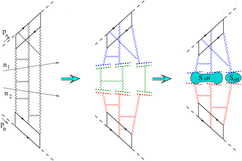
Figure 24: The effective action for the interval of rapidities $\eta_{0}>\eta>\eta^{\prime}_{0}$. The two vectors $n$ and $n^{\prime}$ correspond to “rapidity divides” $\eta_{0}$ and $\eta^{\prime}_{0}$ bordering our chosen region of rapidities.

(For brevity, we do not display the quark fields.) In this formula the operators $V_{i}$ (made from ${\cal A}$ fields) are given by Eq. (4.1), the operators $Y_{i}$ are also given by Eq. (4.1) but constructed from the ${\cal C}$ fields instead, and the operators $W_{i}$ (made from ${\cal C}$ fields) and $U_{i}$ (made from ${\cal B}$ fields) are aligned along the direction $n^{\prime}=\sigma^{\prime}p_{1}+\tilde{\sigma}^{\prime}p_{2}$ corresponding to the rapidity $\eta^{\prime}$ (as usual, $\ln\sigma^{\prime}/\tilde{\sigma}^{\prime}=\eta^{\prime}$ where $\tilde{\sigma}^{\prime}=m^{2}/s\sigma^{\prime}$),

$$V_{i}({\cal A})_{x_{\perp}} = \int^{\infty}_{-\infty}dv[-\infty n,vn]_{x}n^{\mu}F_{\mu i}(vn+x_{\perp})[vn,-\infty n]_{x},$$

$$Y_{i}({\cal C})_{x_{\perp}} = \int^{\infty}_{-\infty}dv[-\infty n,vn]_{x}n^{\mu}F_{\mu i}(vn+x_{\perp})[vn,-\infty n]_{x},$$

$$W_{i}({\cal C})_{x} = \int^{\infty}_{-\infty}dv[-\infty n^{\prime},vn^{\prime}]_{x}n^{{}^{\prime}\mu}F_{\mu i}(vn^{\prime}+x_{\perp})[vn^{\prime},-\infty n^{\prime}]_{x},$$

$$U_{i}({\cal B})_{x_{\perp}} = \int^{\infty}_{-\infty}dv[-\infty n^{\prime},vn^{\prime}]_{x}n^{{}^{\prime}\mu}F_{\mu i}(vn^{\prime}+x_{\perp})[vn^{\prime},-\infty n^{\prime}]_{x}.$$

In conclusion, we have factorized the functional integral over “old” ${\cal B}$ fields into the product of two integrals over ${\cal C}$ and “new” ${\cal B}$ fields.

Now, let us integrate over the ${\cal C}$ fields and write down the result in terms of an effective action. Formally, one obtains:

$$iA(s,t)=\int\!\!{\cal D}{\cal A}e^{iS({\cal A})}j(p_{A})j(p^{\prime}_{A})\int\!\!{\cal D}{\cal B}e^{iS({\cal B})}j(p_{B})j(p^{\prime}_{B})e^{iS_{\rm eff}(V,U;{\sigma\over\sigma^{\prime}})},$$ (190)

where the effective action for the rapidity interval between $\eta$ and $\eta^{\prime}$ is defined as

$$e^{iS_{\rm eff}(V,U;{\sigma\over\sigma^{\prime}})}=\int\!{\cal D}{\cal C}e^{iS({\cal C})}e^{i\!\int\!d^{2}x_{\perp}V^{ai}(x_{\perp})Y^{a}_{i}(x_{\perp})+i\!\int\!d^{2}x_{\perp}W^{ai}(x_{\perp})U^{a}_{i}(x_{\perp})},$$ (191)

($U_{i}\equiv U^{\dagger}{i\over g}\partial_{i}U$ and $V_{i}\equiv V^{\dagger}{i\over g}\partial_{i}V$ as usually). This formula gives a rigorous definition for the effective action for a given interval in rapidity.

Next step would be to perform explicitly the integrations over the longitudinal momenta in the right-hand side of Eq. (191) and obtain the answer for the integration over our rapidity region (from $\eta_{0}$ to $\eta^{\prime}_{0}$) in terms of two-dimensional theory in the transverse coordinate space, hopefully resulting in the unitarization of the BFKL pomeron. At present, the known how to do this. One can obtain, however, a first few terms in the expansion of effective action in powers of $V_{i}$ and $U_{i}$. The easiest way to do this is to expand gauge factors $Y_{i}$ and $W_{i}$ in right-hand side of Eq. (191) in powers of ${\cal C}$ fields and calculate the relevant perturbative diagrams (see Fig. 25).

Figure 25: Lowest order terms in the perturbative expansion of the effective action.

The first few terms in the effective action at the one-log level 

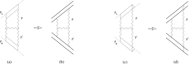
Figure 26: Counting of loops for Feynman diagrams (a),(c) and the corresponding Wilson-line operators (b),(d).

have the form:[3, 22]

$$S_{\rm eff}~{}=~{}\int d^{2}xV^{ai}(x)U^{a}_{i}(x)$$ (192)

$$-~{}{g^{2}\over 64\pi^{3}}\ln{\sigma\over\sigma^{\prime}}\Bigg{(}N_{c}\int d^{2}xd^{2}yV^{a}_{i,i}(x)\ln^{2}(x-y)^{2}U^{a}_{j,j}(y)$$

$$+~{}{f_{abc}f_{mnc}\over 4\pi^{2}}\!\int\!d^{2}xd^{2}yd^{2}x^{\prime}d^{2}y^{\prime}d^{2}zV^{a}_{i,i}(x)V^{m}_{j,j}(y)U^{b}_{k,k}(x^{\prime})U^{n}_{l,l}(y^{\prime})$$

$$\ln{(x-z)^{2}\over(x-x^{\prime})^{2}}\ln{(y-z)^{2}\over(y-y^{\prime})^{2}}\left({\partial\over\partial z_{i}}\right)^{2}\ln{(x^{\prime}-z)^{2}\over(x-x^{\prime})^{2}}\ln{(y^{\prime}-z)^{2}\over(y-y^{\prime})^{2}}\Bigg{)}+\ldots,$$

where we we use the notation $V^{a}_{i,j}(x)\equiv{\partial\over\partial x_{j}}V^{a}_{i}(x)$ etc. The first term (see Fig. 25a) looks like the corresponding term in the factorization formula (4.1), only the directions of the supporting lines are now strongly different. The second term shown in Fig. 25c is the first-order expression for the reggeization of the gluon (74) and the third term (see Fig. 25d) is the gluon emission term in the BFKL kernel (36) in the impact parameter representation.

Let us discuss subsequent terms in the perturbative expansion (192). There can be two types of the logarithmical contributions. First is the “true” loop contribution coming from the diagrams of the Fig. 27a type. This diagram is an iteration of the Lipatov’s Hamiltonian. In addition, in the same $(\ln{\sigma\over\sigma^{\prime}})^{2}$ order there is another contribution coming from the diagram shown in Fig. 27b.

Figure 27: Typical perturbative diagrams in the next $\left(\ln{\sigma\over\sigma^{\prime}}\right)^{2}$ order.

In perturbation theory, these two contributions are of the same order of magnitude.

The situation is different for the case of scattering of two heavy nuclei. Assuming that the effective coupling constant is still small due to the high density,[4] we see that $g\ll 1$, yet the sources are strong ($\sim{1\over g}$) so $gU_{i}\sim gY_{i}\sim 1$. In this case, the diagram in Fig. 27a has the order $g^{4}U_{i}^{2}V_{i}^{2}\left(\ln{\sigma\over\sigma^{\prime}}\right)^{2}\sim\left(\ln{\sigma\over\sigma^{\prime}}\right)^{2}$ while the “tree” Fig. 25b diagram is

$$\sim g^{4}U_{i}^{3}V_{i}^{3}\left(\ln{\sigma\over\sigma^{\prime}}\right)^{2}\sim{1\over g^{2}}\left(\ln{\sigma\over\sigma^{\prime}}\right)^{2}.$$ (193)

In this approximation, first we shall sum up the tree diagrams. As usual, the best way do this is to use the semiclassical method which will be discussed in Sec. 5. In the next paragraph we will consider the intermediate situation with one weak source and one strong source.

4.3 Effective action for one weak and one strong source

Consider again the DIS from a nucleon or nucleus where the high-energy behavior is governed by the non-linear evolution equation (136). In this section we will translate the evolution results (152) into the effective action language (see also Refs. 52, 53). In the case DIS one of the sources (corresponding to quark-antiquark pair) is weak while the other (describing the nucleon or nuclei) is strong.

For example, if the source $V_{i}$ is weak (and hence $gV_{i}$ is a valid small parameter) but the source $U_{i}$ is not weak (so that $gV_{i}\sim 1$ is not a small parameter), one must take into account the diagrams shown in Fig. 28a and b.

Figure 28: Perturbative diagrams for the effective action in the case of one weak source and one strong one.

The multiple rescatterings in Fig. 28a,b describe the motion of the gluon emitted by the weak source $V_{i}$ in the strong external field $A_{i}=U_{i}\theta(x_{\ast})$ created by the source $U_{i}$. The result of the calculation of the diagram in Fig. 28a presented in a form of the evolution of the Wilson-line operators $U_{i}$ can be easily obtained using the evolution equations (299)

$$U^{a}_{i}(x_{\perp})\!\! \rightarrow \!\!U^{a}_{i}(x_{\perp})$$

$$- \!\!{g^{2}\over 8\pi^{3}}\ln{\sigma\over\sigma^{\prime}}\int dy_{\perp}{1\over(\vec{x}-\vec{y})_{\perp}^{2}}\Big{(}f^{abc}\big{(}U^{\dagger}_{x}\partial_{i}U_{y}\big{)}^{bc}+N_{c}U^{a}_{i}(x_{\perp})\Big{)}+\ldots,$$

where dots stand for the terms with higher powers of $g^{2}\ln{\sigma\over\sigma^{\prime}}$. This evolution equation means that if we integrate over the rapidities $\eta_{0}>\eta>\eta^{\prime}_{0}$ in the matrix elements of the operator $Y_{i}$ we will get the expression (4.3) constructed from the operators $U_{i}$ with rapidities up to $\eta^{\prime}_{0}$ times factors proportional to $g^{2}(\eta_{0}-\eta^{\prime}_{0})\equiv g^{2}\ln{\sigma\over\sigma^{\prime}}$. Therefore, the corresponding contribution to the effective action at the one-log level takes the form

$$\int dx_{\perp}V^{a}_{i}(x_{\perp})U^{ai}(x_{\perp})~{}~{}\rightarrow~{}~{}\int dx_{\perp}V^{a}_{i}(x_{\perp})U^{ai}(x_{\perp})$$ (195)

$$+~{}{g^{2}\over 8\pi^{3}}\ln{\sigma\over\sigma^{\prime}}\int\!dx_{\perp}dy_{\perp}{1\over(\vec{x}-\vec{y})_{\perp}^{2}}\Big{(}i\big{(}V^{i}(x_{\perp})U^{\dagger}_{x}\partial_{i}U_{y}\big{)}^{aa}-N_{c}V^{ai}(x_{\perp})U^{a}_{i}(x_{\perp})\Big{)}$$

where the first term is the lowest-order effective action ($\equiv$ the first term in Eq. (192)) and the second term contains new information. To check the second term, we may expand it in powers of the source $U_{i}$, then it is easy to see that the first nontrivial term in this expansion coincides with the gluon-reggeization term in Eq. (192).

Apart from the (195) term, there is another contribution to the one-loop evolution equations coming from the diagrams in Fig. 28b. It can be easily obtained using formulas (7.3) from the Appendix,

$$\!\!\!\!U_{i}^{a}(x_{\perp})U_{j}^{b}(y_{\perp})\rightarrow-{g^{2}\over 4\pi^{3}}\ln{\sigma\over\sigma^{\prime}}$$

$$\times \Big{(}\nabla^{x}_{i}\Big{[}\int dz_{\perp}{(\vec{x}-\vec{z},\vec{y}-\vec{z})_{\perp}\over(\vec{x}-\vec{z})_{\perp}^{2}(\vec{y}-\vec{z})_{\perp}^{2}}(U^{\dagger}_{x}U_{y}+1-U^{\dagger}_{x}U_{z}-U^{\dagger}_{z}U_{y})\Big{]}\stackrel{{\scriptstyle\leftarrow}}{{\nabla}}^{y}_{j}\Big{)}^{ab},$$

where

$$\nabla^{x}_{i}{\cal O}(x_{\perp}) \equiv {\partial\over\partial x^{i}}{\cal O}(x_{\perp})-iU_{i}(x_{\perp}){\cal O}(x_{\perp}),$$

$${\cal O}(y_{\perp})\stackrel{{\scriptstyle\leftarrow}}{{\nabla}}^{y}_{i} \equiv -{\partial\over\partial y^{i}}{\cal O}(y_{\perp})-i{\cal O}(y_{\perp})U_{i}(y_{\perp}),$$ (197)

are the “covariant derivatives” (in the adjoint representation). The corresponding term in effective action is

$$\!\!\!\!{ig^{2}\over 8\pi^{3}}\ln{\sigma\over\sigma^{\prime}}\int dx_{\perp}dy_{\perp}\left(\nabla^{x}_{i}V^{a}_{i}\right)(x_{\perp})\int dz_{\perp}{(\vec{x}-\vec{z},\vec{y}-\vec{z})_{\perp}\over(\vec{x}-\vec{z})_{\perp}^{2}(\vec{y}-\vec{z})_{\perp}^{2}}$$ (198)

$$\times \big{(}U^{\dagger}_{x}U_{y}+1-U^{\dagger}_{x}U_{z}-U^{\dagger}_{z}U_{y}\big{)}^{ab}\left(\nabla^{y}_{j}V^{b}_{j}\right)(y_{\perp}).$$

The final form of the one-log effective action for this case is the sum of the expressions (195) and (198),

$$\!\!\!\!S^{(I)}_{\rm eff}(V_{i},U_{j})=\int d^{2}xV^{ai}(x)U^{a}_{i}(x)+{g^{2}\over 8\pi^{3}}\ln{\sigma\over\sigma^{\prime}}\int\!dx_{\perp}dy_{\perp}{1\over(\vec{x}-\vec{y})_{\perp}^{2}}$$ (199)

$$\times \Big{(}i\big{(}V^{i}(x_{\perp})U^{\dagger}_{x}\partial_{i}U_{y}\big{)}^{aa}-N_{c}V^{ai}(x_{\perp})U^{a}_{i}(x_{\perp})\Big{)}$$

$$+ {ig^{2}\over 8\pi^{3}}\ln{\sigma\over\sigma^{\prime}}\int dx_{\perp}dy_{\perp}\nabla^{x}_{i}V^{ai}(x_{\perp})\int dz_{\perp}{(\vec{x}-\vec{z})_{\perp}\cdot(\vec{y}-\vec{z})_{\perp}\over(\vec{x}-\vec{z})_{\perp}^{2}(\vec{y}-\vec{z})_{\perp}^{2}}$$

$$\times \big{(}U^{\dagger}_{x}U_{y}+1-U^{\dagger}_{x}U_{z}-U^{\dagger}_{z}U_{y}\big{)}^{ab}\nabla^{y}_{j}V^{bj}(y_{\perp}),$$

where $V_{i}$ is a weak source and $U_{i}$ is a strong one. It is clear that if the source $V_{i}$ is strong and $U_{i}$ is weak diagrams the effective action $S^{(II)}_{\rm eff}(V_{i},U_{j})$ will have the similar form with the replacement $V\leftrightarrow U$ coming from the diagram shown in Fig. 29.

Figure 29: Effective action for the strong source $V$ and the weak source $U$.

As we mentioned above, in the case of two strong sources the $\left(\ln{\sigma\over\sigma^{\prime}}\right)^{2}$ terms start from the diagram shown in Fig. 27b (see Eq. (193)), hence Fig. 27 and Fig. 29 complete the list of diagrams which contribute to the effective action at the one-log level. Higher-order diagrams start from higher powers of $\ln{\sigma\over\sigma^{\prime}}$. The analog of LLA here is a cluster expansion with the parameter $(U-1)(V-1)\ln{\sigma\over\sigma^{\prime}}$ shown in Fig. 30.

Figure 30: Cluster expansion of the effective action.

Of course, the diagrams of Fig. 30 give the terms $\sim\ln{\sigma\over\sigma^{\prime}}$ too, but in the leading order the kernel of the corresponding evolution equation is determined by Fig. 27 and Fig. 28. Thus, the one-log answer for two strong sources can be guessed by comparison of the answers for $S_{\rm eff}(V_{i},U_{j})$ with $V_{i}\sim 1,~{}U_{i}\sim{1\over g}$ and with $U_{i}\sim 1,~{}V_{i}\sim{1\over g}$. Instead of doing that, we will obtain the one-log result for two strong sources using the semiclassical method and check that it agrees with (199).

It means that the one-log answer in the general case can be guessed by comparison of the answers for $S_{\rm eff}(V_{i},U_{j})$ with $V_{i}\sim 1,~{}U_{i}\sim{1\over g}$ and with $U_{i}\sim 1,~{}V_{i}\sim{1\over g}$ Instead of doing that, we will obtain the one-log result for two strong sources using the semiclassical method and check that it agrees with (199).

5 High-energy effective action in sQCD

5.1 Effective action and collision of two shock waves

The functional integral (191) which defines the effective action is the usual QCD functional integral with two sources corresponding to the two colliding shock waves, see Fig. 31.[54]

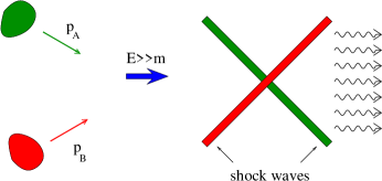
Figure 31: Scattering of two shock waves.

Instead of calculation of perturbative diagrams we can use the semiclassical approach which is relevant when the coupling constant is relatively small but the characteristic fields are large – in other words, when $g^{2}\ll 1$ but $gV_{i}\sim gU_{i}\sim 1$. As was discussed in Ref. 4, this situation is realized in the heavy-ion collisions where the coupling constant is defined by the parton saturation scale $Q_{s}$, which is estimated to be $\sim 1$ GeV at RHIC and $\sim 2-3$ GeV at LHC.[6, 7] Even if we consider the $\gamma^{\ast}\gamma^{\ast}$ scattering, the number of gluons in the middle of the rapidity region may become very large leading to the saturation at high energies so in the middle of the rapidity region we will se the scattering of two strong shock waves.

If both sources are strong, one can calculate the functional integral (191) by expansion around the new stationary point corresponding to the classical wave created by the collision of the shock waves. With leading log accuracy, we can replace the vector $n$ by $p_{1}$ and the vector $n^{\prime}$ by $p_{2}$. Then the functional integral (191) takes the form

$$e^{iS_{\rm eff}(V,U;{\sigma\over\sigma^{\prime}})}=\int\!{\cal D}Ae^{iS_{QCD}(A)}e^{i\!\int\!d^{2}x_{\perp}V^{ai}(x_{\perp})Y^{a}_{i}(x_{\perp})+i\!\int\!d^{2}x_{\perp}W^{ai}U^{a}_{i}(x_{\perp})},$$ (200)

where now

$$Y^{a}_{i}(x_{\perp})=\int^{\infty}_{-\infty}dv\hat{F}_{\bullet i}(vp_{1}+x_{\perp}),\qquad W^{a}_{i}=\int^{\infty}_{-\infty}dv\tilde{F}_{\ast i}(vp_{2}+x_{\perp}).$$ (201)

Hereafter we use the notations

$$\hat{\cal O}(x) = [-\infty p_{1}+x,x]{\cal O}(x)[x,-\infty p_{1}+x],$$

$$\tilde{\cal O}(x) = [-\infty p_{2}+x,x]{\cal O}(x)[x,-\infty p_{2}+x].$$ (202)

Note that we changed the name for the gluon fields in the integrand from ${\cal C}$ back to $A$.

As usual, the classical equation for the saddle point $\bar{A}$ in the functional integral (200) is

$$\left.{\delta\over\delta A}\left(S_{QCD}+\!\int\!d^{2}x_{\perp}V^{ai}(x_{\perp})Y^{a}_{i}(x_{\perp})+\!\int\!d^{2}x_{\perp}W^{ai}U^{a}_{i}(x_{\perp}\right)\right|_{A=\bar{A}}=0.$$ (203)

To write them down explicitly we need the first variational derivatives of the source terms with respect to gauge field. We have:

$$\delta Y_{i}=\delta\hat{A}_{i}(\infty p_{1}+x_{\perp})-\delta{A}_{i}(-\infty p_{1}+x_{\perp})-\int^{\infty}_{-\infty}du\hat{\nabla}_{i}\delta\hat{A}_{i}(up_{1}+x_{\perp}),$$

$$\delta W_{i}=\delta\tilde{A}_{i}(\infty p_{2}+x_{\perp})-\delta{A}_{i}(-\infty p_{2}+x_{\perp})-\int^{\infty}_{-\infty}du\tilde{\nabla}_{i}\delta\tilde{A}_{i}(up_{2}+x_{\perp}),$$ (204)

where

$$\hat{\nabla}_{i}{\cal O}(x) \equiv \partial_{i}{\cal O}(x)-i[Y_{i}(x_{\perp})+A_{i}(-\infty p_{1}+x_{\perp}),{\cal O}(x)],$$

$$\tilde{\nabla}_{i}{\cal O}(x) \equiv \partial_{i}{\cal O}(x)-i[W_{i}(x_{\perp})+A_{i}(-\infty p_{2}+x_{\perp}),{\cal O}(x)].$$ (205)

Therefore the explicit form of the classical equations (203) for the wave created by the collision is

$$D^{\mu}{\bar{F}}_{\mu i} = 0,$$ (206)

$$D^{\mu}{\bar{F}}_{\ast\mu} = \delta({2\over s}x_{\bullet})[{2\over s}x_{\ast}p_{1},-\infty p_{1}]_{x_{\perp}}\hat{\nabla}_{i}V^{i}(x_{\perp})[-\infty p_{1},{2\over s}x_{\ast}p_{1}]_{x_{\perp}},$$

$$D^{\mu}{\bar{F}}_{\bullet\mu} = \delta({2\over s}x_{\ast})[{2\over s}x_{\bullet}p_{2},-\infty p_{2}]_{x_{\perp}}\tilde{\nabla}_{i}U^{i}(x_{\perp})[-\infty p_{2},{2\over s}x_{\bullet}p_{2}]_{x_{\perp}}.$$

These equations define the classical field created by the collision of two shock waves. Unfortunately, it is not clear how to solve these equations. One can start with the trial field which is a superposition of the two shock waves (169), and improve it by taking into account the interaction between the shock waves order by order.[3] The parameter of this expansion is the commutator $g^{2}[U_{i},V_{k}]$. Actually, there are two independent commutators,

$$L_{1}=L_{1}^{a}t^{a},\qquad L^{a}_{1}=if^{abc}U^{a}_{j}V^{bj},$$

$$L_{2}=L_{2}^{a}t^{a},\qquad L^{a}_{2}=i\epsilon_{ik}f_{abc}U^{bi}V^{ck},$$ (207)

where $\epsilon_{ik}$ is the totally antisymmetric tensor in two transverse dimensions ($\epsilon_{12}=1$). In these notations $[U_{i},V^{i}]=L_{1}$ and $[U_{i},V_{k}]-(i\leftrightarrow k)=\epsilon_{ik}L_{2}$. It can be demonstrated that each extra commutator brings a factor $\ln{\sigma\over\sigma^{\prime}}$ (each commutator means higher term in the cluster expansion in Fig. 30), thus this approach is a kind of LLA. It is convenient to choose the trial field in the form 

$${\bar{A}}^{(0)}_{\ast}={\bar{A}}^{(0)}_{\bullet}=0,\qquad{\bar{A}}^{(0)}_{i}=\theta(x_{\bullet})V_{i}+\theta(x_{\ast})U_{i}+\theta(x_{\bullet})\theta(x_{\ast})\Delta_{i}$$ (208)

where $\Lambda_{i}(x_{\perp})=U_{i}(x_{\perp})+V_{i}(x_{\perp})+\Delta_{i}(x_{\perp})$ is a pure gauge field satisfying the gauge condition $\partial_{i}\Delta_{i}-i[\Lambda_{i},\Delta_{i}]=0$. The explicit form of $\Delta_{i}$ is

$$\Delta^{i}(x_{\perp}) = ig\epsilon^{ik}\big{(}U^{\dagger}{\partial_{k}\over\vec{\partial}_{\perp}^{2}}U+V^{\dagger}{\partial_{k}\over\vec{\partial}_{\perp}^{2}}V-{\partial_{k}\over\vec{\partial}_{\perp}^{2}}\big{)}L_{2}+O(L^{2})$$

$$= -ig\int dz_{\perp}{\epsilon^{ik}(x-z)_{k}\over 2\pi(\vec{x}-\vec{z})_{\perp}^{2}}(U_{x}U^{\dagger}_{z}+V_{x}V^{\dagger}_{z}-1)L_{2}(z_{\perp})dz_{\perp}+O(L^{2}).$$

In the first nontrivial order one gets:

$${\bar{A}}^{(1)}_{i} = -{i\over 2\pi^{2}}\int dz_{\perp}{1\over-x_{\parallel}^{2}+(\vec{x}-\vec{z})_{\perp}^{2}+i\epsilon}\Delta_{i}(z_{\perp})$$

$$= -{g\over 4\pi^{2}}\int dz_{\perp}{\epsilon_{ik}(x-z)^{k}\over(\vec{x}-\vec{z})_{\perp}^{2}}\ln\left(1-{(\vec{x}-\vec{z})_{\perp}^{2}\over x_{\parallel}^{2}+i\epsilon}\right)L_{2}(z_{\perp}),$$

$${\bar{A}}^{(1)}_{\bullet} = {gs\over 16\pi^{2}}\int dz_{\perp}{1\over x_{\ast}+i\epsilon}\ln(-x_{\parallel}^{2}+(\vec{x}-\vec{z})_{\perp}^{2}+i\epsilon)L_{1}(z_{\perp}),$$

$${\bar{A}}^{(1)}_{\ast} = -{gs\over 16\pi^{2}}\int dz_{\perp}{1\over x_{\bullet}+i\epsilon}\ln(-x_{\parallel}^{2}+(\vec{x}-\vec{z})_{\perp}^{2}+i\epsilon)L_{1}(z_{\perp}),$$ (210)

where $x_{\parallel}^{2}\equiv{4\over s}x_{\ast}x_{\bullet}$ is a longitudinal part of $x^{2}$. These fields are obtained in the background-Feynman gauge. The corresponding expressions for field strength have the form

$${\bar{F}}^{(1)}_{\bullet\ast} = {gs\over 4\pi^{2}}\int dz_{\perp}{1\over-x_{\parallel}^{2}+(\vec{x}-\vec{z})_{\perp}^{2}+i\epsilon}L_{1}(z_{\perp}),$$ (211)

$${\bar{F}}^{(1)}_{ik} = {g\over 2\pi^{2}}\epsilon_{ik}\int dz_{\perp}{1\over-x_{\parallel}^{2}+(\vec{x}-\vec{z})_{\perp}^{2}+i\epsilon}L_{2}(z_{\perp}),$$

$${\bar{F}}^{(1)}_{\bullet i} = {gs\over 8\pi^{2}}\!\int\!dz_{\perp}{(x-z)^{k}\over-x_{\parallel}^{2}+(\vec{x}-\vec{z})_{\perp}^{2}+i\epsilon}\left({g_{ik}L_{1}(z_{\perp})\over x_{\ast}-i\epsilon}+{\epsilon_{ik}L_{2}(z_{\perp})\over x_{\ast}+i\epsilon}\right)$$

$$- i[{\bar{A}}^{(1)}_{\bullet},{\bar{A}}^{(0)}_{i}],$$

$${\bar{F}}^{(1)}_{\ast i} = -{gs\over 8\pi^{2}}\!\int\!dz_{\perp}{(x-z)^{k}\over-x_{\parallel}^{2}+(\vec{x}-\vec{z})_{\perp}^{2}+i\epsilon}\left({g_{ik}L_{1}(z_{\perp})\over x_{\bullet}-i\epsilon}-{\epsilon_{ik}L_{2}(z_{\perp})\over x_{\bullet}+i\epsilon}\right)$$

$$- i[{\bar{A}}^{(1)}_{\ast},{\bar{A}}^{(0)}_{i}].$$

In terms of usual Feynman diagrams (when we expand in powers of source just like in Sec. 4.2) these expressions come from the diagrams shown in Fig. 32.

Figure 32: Perturbative Feynman diagrams for the field strength (211).

When we sum up the three contributions from the diagrams in Figs. 32a, 32b, and 32c the three-gluon vertex in Fig. 32a is replaced by the effective Lipatov’s vertex (30) and we get (211) up to the terms ${1\over\partial^{2}}\partial_{i}\partial_{k}U^{k}$ and ${1\over\partial^{2}}\partial_{j}\partial_{k}V^{k}$ standing in place of $U_{i}$ and $V_{j}$. However, as we have discussed in Sec. 3, the difference $U_{i}-{1\over\partial^{2}}\partial_{i}\partial_{k}U^{k}=g{\partial_{k}\over\partial^{2}}[U_{i},U_{k}]$ (which has an additional power of g) will be canceled by the next-order perturbative diagrams of the Fig. 32d type.

Let us now find the effective action

$$\bar{S}_{\rm eff}=S_{QCD}(\bar{A})+\!\int\!d^{2}x_{\perp}V^{ai}(x_{\perp})\bar{Y}^{a}_{i}(x_{\perp})+\!\int\!d^{2}x_{\perp}\bar{W}^{ai}U^{a}_{i}(x_{\perp})$$ (212)

in the semiclassical approximation. In the trivial order the only non-zero field strength components are ${\bar{F}}^{(0)}_{\bullet i}=\delta({2\over s}x_{\ast})U_{i}(x_{\perp})$ and ${\bar{F}}^{(0)}_{\ast i}=\delta({2\over s}x_{\bullet})V_{i}(x_{\perp})$, hence we get the familiar expression $S^{(0)}=\int d^{2}x_{\perp}V^{ai}U^{a}_{i}$. In the next order one has

$$S^{(1)}~{}=~{}\int d^{4}x\left(-{2\over s}{\bar{F}}_{\ast}^{(1)ai}{\bar{F}}^{(1)a}_{\bullet i}-{1\over 4}{\bar{F}}^{(1)a}_{ik}{\bar{F}}^{(1)aik}+{2\over s^{2}}{\bar{F}}^{(1)a}_{\ast\bullet}{\bar{F}}^{(1)a}_{\ast\bullet}\right)$$

$$+~{}2\!\int\!d^{2}x_{\perp}\int\!du\Big{(}{\rm Tr}V^{i}\left([-\infty p_{1},up_{1}]_{x}{\bar{F}}_{\bullet i}(up_{1}+x_{\perp})[up_{1},-\infty p_{1}]_{x}\right)^{(1)}$$

$$+~{}{\rm Tr}U^{i}\left([-\infty p_{2},up_{2}]_{x}{\bar{F}}_{\ast i}(up_{2}+x_{\perp})[up_{2},\infty p_{2}]_{x}\right)^{(1)}\Big{)}.$$ (213)

Above, we have seen that the effective action contains $\ln{\sigma\over\sigma^{\prime}}$ (see Eq. (192)). With logarithmic accuracy, the right-hand side of Eq. (213) reduces to

$$S^{(1)} = -{2\over s}\int d^{4}x{\bar{F}}^{(1)ai}_{\ast}(x){\bar{F}}_{\bullet i}^{(1)a}(x).$$

$$+ \int d^{2}x_{\perp}2{\rm Tr}L_{1}(x_{\perp})\left([x_{\perp},-\infty p_{2}+x_{\perp}]^{(1)}-[x_{\perp},-\infty p_{1}+x_{\perp}]^{(1)}\right).$$

The first term contains the integral over $d^{4}x={2\over s}dx_{\bullet}dx_{\ast}d^{2}x_{\perp}$. In order to separate the longitudinal divergencies from the infrared divergencies in the transverse space we will work in the $d=2+2\epsilon$ transverse dimensions. It is convenient first to perform the integral over $x_{\ast}$ determined by a residue in the point $x_{\ast}=0$. The integration over remaining light-cone variable $x_{\bullet}$ then factorizes in the form $\int_{0}^{\infty}dx_{\bullet}/x_{\bullet}$ or $\int_{-\infty}^{0}dx_{\bullet}/x_{\bullet}$. This integral reflects our usual longitudinal logarithmic divergencies, which arise from the replacement of vectors $n$ and $n^{\prime}$ in (191) by the light-like vectors $p_{1}$ and $p_{2}$. In the momentum space this logarithmical divergency has the form $\int d\alpha/\alpha$. It is clear that when $\alpha$ is close to $\sigma$ (or $\sigma^{\prime}$) we can no longer approximate $n$ by $p_{1}$ (or $n^{\prime}$ by $p_{2}$). Therefore, in the leading log approximation this divergency should be replaced by $\ln{\sigma\over\sigma^{\prime}}$,

$$\int_{0}^{\infty}dx_{\bullet}{1\over x_{\bullet}}=\int_{0}^{\infty}d\alpha{1\over\alpha}\rightarrow\int_{\sigma}^{\sigma^{\prime}}d\alpha{1\over\alpha}~{}=~{}\ln{\sigma\over\sigma^{\prime}}.$$ (215)

The (first-order) gauge links in the second term in the right-hand side of Eq. (5.1) have the logarithmic divergence of the same origin,

$$\![x_{\perp},-\infty p_{1}+x_{\perp}]^{(1)} = -{i\over 8\pi^{2}}\int^{0}_{-\infty}\!{dx_{\ast}\over x_{\ast}}\int d^{2}z_{\perp}{\Gamma(\epsilon)\over(\vec{x}-\vec{z})_{\perp}^{2\epsilon}}L_{1}(z_{\perp}),$$

$$\![x_{\perp},-\infty p_{2}+x_{\perp}]^{(1)} = {i\over 8\pi^{2}}\int^{0}_{-\infty}\!{dx_{\bullet}\over x_{\bullet}}\int d^{2}z_{\perp}{\Gamma(\epsilon)\over(\vec{x}-\vec{z})_{\perp}^{2\epsilon}}L_{1}(z_{\perp}),$$ (216)

which should also be replaced by $\ln{\sigma\over\sigma^{\prime}}$. Performing the remaining integration over $x_{\perp}$ in the first term in right-hand side of Eq. (5.1) we obtain the the first-order classical action in the form

$$S^{(1)} = -{ig^{2}\over 8\pi^{2}}\ln{\sigma\over\sigma^{\prime}}$$

$$\times \int d^{2}x_{\perp}d^{2}y_{\perp}\big{(}L^{a}_{1}(x_{\perp})L^{a}_{1}(y_{\perp})+L^{a}_{2}(x_{\perp})L^{a}_{2}(y_{\perp})\big{)}{\Gamma(\epsilon)\over(\vec{x}-\vec{y})_{\perp}^{2\epsilon}}$$

or

$$S^{(1)}={ig^{2}\over 2\pi}\ln{\sigma\over\sigma^{\prime}}\int d^{2}x_{\perp}\left(L_{1}^{a}{1\over\vec{\partial}_{\perp}^{2}}L_{1}^{a}+L_{2}^{a}{1\over\vec{\partial}_{\perp}^{2}}L_{2}^{a}\right).$$ (219)

Note that in the trivial order the three terms in Eq. (212) are equal up to the different sign of the $S(\bar{A})$ term. It can be demonstrated that this is true in the first order, too:

$$\int d^{2}x_{\perp}2{\rm Tr}V^{i}\bar{Y}_{i}^{(0+1)}=\int d^{2}x_{\perp}2{\rm Tr}\bar{W}_{i}^{(0+1)}U_{i}=-S(\bar{A})^{(0+1)}.$$ (220)

A more accurate version of Eq. (219) has the form (see Appendix 7.5)

$$S^{(1)} = {ig^{2}\over 2\pi}\ln{\sigma\over\sigma^{\prime}}\int d^{2}x_{\perp}$$

$$\times \Bigg{(}L_{1}^{a}{1\over\vec{\partial}_{\perp}^{2}}L_{1}^{a}+L_{2}^{a}\big{(}U^{\dagger}{1\over\vec{\partial}_{\perp}^{2}}U+V^{\dagger}{1\over\vec{\partial}_{\perp}^{2}}V-{1\over\vec{\partial}_{\perp}^{2}}\big{)}^{ab}L_{2}^{b}$$

$$+ L_{1}^{a}\big{(}{\partial_{i}\over\vec{\partial}_{\perp}^{2}}U^{\dagger}{\partial_{k}\over\vec{\partial}_{\perp}^{2}}U-U\leftrightarrow V\big{)}L^{b}_{2}\epsilon^{ik}$$

$$- L_{2}^{a}\epsilon^{ik}\big{(}U^{\dagger}{\partial_{i}\over\vec{\partial}_{\perp}^{2}}U{\partial_{k}\over\vec{\partial}_{\perp}^{2}}-U\leftrightarrow V\big{)}^{ab}L^{b}_{1}\Bigg{)}+O([U,V]^{3}).$$

It is easy to see that in the case of one weak and one strong source this expressions coincides with (198) (up to the terms of higher order in weak source which we neglect anyway).

At $d=2$ we have an infrared pole in $S^{(1)}$ which must be canceled by the corresponding divergency in the trajectory of the reggeized gluon. The gluon reggeization is not a classical effect in our approach, rather it is a quantum correction coming from the loop corresponding to the determinant of the operator of second derivative of the action

$$\left.{\delta\over\delta A_{\mu}}{\delta\over\delta A_{\nu}}\left(S_{QCD}+\!\int\!d^{2}x_{\perp}V^{ai}(x_{\perp})Y^{a}_{i}(x_{\perp})+\!\int\!d^{2}x_{\perp}W^{ai}U^{a}_{i}(x_{\perp}\right)\right|_{A=\bar{A}}.$$ (222)

The lowest-order diagrams are shown in Fig. 33

Figure 33: Lowest-order diagrams for gluon reggeization.

and the explicit form of the second derivative of the Wilson-line operator is

$$\delta Y_{i} = i\int^{\infty}_{-\infty}du\int^{u}_{-\infty}dv[\delta\hat{A}_{i}(up_{1}+x_{\perp}),\hat{\nabla}_{i}\delta\hat{A}_{i}(vp_{1}+x_{\perp})],$$

$$\delta W_{i} = i\int^{\infty}_{-\infty}du\int^{u}_{-\infty}dv[\tilde{A}_{i}(up_{2}+x_{\perp}),\tilde{\nabla}_{i}\delta\tilde{A}_{i}(up_{2}+x_{\perp})].$$ (223)

Now one easily gets the contribution of the Fig. 33 diagrams in the form

$$S_{\rm r} = {g^{2}N_{c}\over 8\pi^{3}}\ln{\sigma\over\sigma^{\prime}}\int d^{2}x_{\perp}d^{2}y_{\perp}$$

$$\times \Big{(}V_{i}^{a}(x_{\perp})U^{ai}(y_{\perp})-V_{i}^{a}(x_{\perp})U^{ai}(x_{\perp})\Big{)}{\Gamma^{2}(1+\epsilon)\over((\vec{x}-\vec{y})_{\perp}^{2})^{(1+2\epsilon)}}.$$

A more accurate form of this equation reads:

$$S_{\rm r} = {g^{2}N_{c}\over 8\pi^{3}}\ln{\sigma\over\sigma^{\prime}}\int d^{2}x_{\perp}d^{2}y_{\perp}{\Gamma^{2}(1+\epsilon)\over((\vec{x}-\vec{y})_{\perp}^{2})^{(1+2\epsilon)}}$$

$$\times \Big{\{}-V_{i}^{a}(x_{\perp})U^{ai}(x_{\perp})+{1\over N_{c}}\Big{(}V^{i}(x_{\perp})\{U(x_{\perp})U^{\dagger}(y_{\perp})$$

$$+ V(x_{\perp})V^{\dagger}(y_{\perp})-1\}U^{i}(y_{\perp})\Big{)}^{aa}\Big{\}}+O([U,V]),$$

where ${\cal O}^{aa}\equiv$Tr$O$ in the gluonic representation. In the case of one strong and one weak source it coincides with (195) (up to the higher powers of weak source).

The complete first-order ($\equiv$ one-log) expression for the effective action is the sum of $S^{(0)}$, $S^{(1)}$, and $S_{\rm r}$,

$$S_{\rm eff}\!\!\! = \!\!\!\int d^{2}xV^{ai}(x)U^{a}_{i}(x)~{}+~{}{ig^{2}\over 8\pi^{2}}\ln{\sigma\over\sigma^{\prime}}\!\int\!d^{2}xd^{2}y\Bigg{\{}-{\Gamma(\epsilon)\over(\vec{x}-\vec{z})_{\perp}^{2\epsilon}}$$

$$\times \!\!\!\Big{(}L^{a}_{1}(x)L^{a}_{1}(y)+L^{a}_{2}(x)L^{b}_{2}(y)\big{(}U^{\dagger}_{x}U_{y}+V^{\dagger}_{x}V_{y}-1\big{)}^{ab}\Big{)}$$

$$+ \!\!\!\int\!d^{2}z{\epsilon^{ij}(x-z)_{i}(z-y)_{j}\over\pi(\vec{x}-\vec{z})_{\perp}^{2}(\vec{z}-\vec{y})_{\perp}^{2}}$$

$$\times \!\!\!\Big{(}L^{a}_{1}(x)\big{(}U^{\dagger}_{z}U_{y}-U\leftrightarrow V\big{)}^{ab}L^{b}_{2}(y)-L^{a}_{2}(x)\big{(}U^{\dagger}_{x}U_{z}-U\leftrightarrow V\big{)}^{ab}L^{b}_{1}(y)\Big{)}\Bigg{\}}$$

$$+ \!\!\!{g^{2}N_{c}\over 8\pi^{3}}\ln{\sigma\over\sigma^{\prime}}\int d^{2}x_{\perp}d^{2}y_{\perp}{\Gamma^{2}(1+\epsilon)\over((\vec{x}-\vec{y})_{\perp}^{2})^{(1+2\epsilon)}}\Bigg{\{}-V_{i}^{a}(x_{\perp})U^{ai}(x_{\perp})$$

$$+ \!\!\!{1\over N_{c}}\Big{(}V^{i}(x_{\perp})\{U(x_{\perp})U^{\dagger}(y_{\perp})+V(x_{\perp})V^{\dagger}(y_{\perp})-1\}U^{i}(y_{\perp})\Big{)}^{aa}\Bigg{\}}.$$

In the case of one weak and one strong source this expression coincides with (199) up to the higher powers of weak source. (As we discussed in Sec. 4.3, the new nontrivial terms in the case of two strong sources start from $[Y,V]^{3}\ln^{2}{\sigma\over\sigma^{\prime}}$).

As usual, in the case of scattering of white objects the logarithmic infrared divergence $\sim{1\over\epsilon}$ cancels. For example, for the case of one-pomeron exchange the relevant term in the expansion of $e^{iS_{\rm eff}}$ has the form

$$-{g^{2}\over 16\pi^{2}}\ln{\sigma\over\sigma^{\prime}}\int d^{2}x_{\perp}d^{2}y_{\perp}f^{dam}(V_{j}^{a}U^{mj}g_{ik}+V^{a}_{i}U^{m}_{k}-V^{a}_{k}U^{m}_{i})(x_{\perp})$$ (227)

$$\times {\Gamma(\epsilon)\over(\vec{x}-\vec{y})_{\perp}^{2\epsilon}}f^{dbn}(V_{l}^{b}U^{nl}g^{ik}+V^{bi}U^{mk}-V^{bk}U^{mi})(y_{\perp})$$

$$+ {g^{2}N_{c}\over 16\pi^{3}}\ln{\sigma\over\sigma^{\prime}}\int d^{2}x_{\perp}V^{a}_{i}(x_{\perp})U^{ai}(x_{\perp})\int d^{2}y_{\perp}d^{2}y^{\prime}_{\perp}(V_{j}^{b}(y_{\perp})-V_{j}^{b}(y^{\prime}_{\perp}))$$

$$\times {\Gamma^{2}(1+\epsilon)\over((\vec{y}-\vec{y}^{\prime})_{\perp}^{2})^{(1+2\epsilon)}}(U^{bj}(y_{\perp})-U^{bj}(y^{\prime}_{\perp})).$$

It is easy to see that the terms $\sim{1\over\epsilon}$ cancel if we project Eq. (227) onto colorless state in t-channel (that is, replace $V^{ai}V_{j}^{b}$ by ${\delta_{ab}\over N_{c}^{2}-1}V^{ci}V_{j}^{c}$). It is worth noting that in the two-gluon approximation the right-hand side of the Eq. (227) gives the BFKL kernel (47).

As an illustration, let us present the next-to-leading contribution to the effective action $\simeq[U,V]^{3}\ln{\sigma\over\sigma^{\prime}}$ coming from the diagrams of Fig. 34 type.

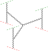
Figure 34: Typical next-to-leading order contribution to $S_{\rm eff}$.

$$S_{\rm eff}\!\! = \!\!g^{3}f_{abc}\ln{\sigma\over\sigma^{\prime}}\int dx_{\perp}dy_{\perp}d_{\perp}z\big{[}K_{1}(x_{\perp},y_{\perp},z_{\perp})L^{a}_{1}(x_{\perp})L_{1}^{b}(y_{\perp})L_{2}^{c}(z_{\perp})$$ (228)

$$+ \!\!K_{2}(x_{\perp},y_{\perp},z_{\perp})L_{2}^{2}(x_{\perp})L_{2}^{b}(y_{\perp})L_{2}^{c}(z_{\perp})\big{]},$$

where

$$K_{i}(x,y,z)=\int{d^{2}p_{1}\over 4\pi^{2}}{d^{2}p_{2}\over 4\pi^{2}}K_{i}(p_{1},p_{2},-p_{1}-p_{2})e^{ip_{1}\cdot(x-z)+ip_{2}\cdot(y-z)},$$

$$K_{1}(p_{1},p_{2},p_{3})={i\over 2\pi^{2}}{\epsilon_{ik}p_{1}^{i}p_{2}^{k}\over p_{1}^{2}p_{2}^{2}p_{3}^{2}}\left(\ln p_{3}^{2}-{p_{1}^{2}\over p_{1}^{2}-p_{2}^{2}}\ln p_{1}^{2}-{p_{2}^{2}\over p_{2}^{2}-p_{1}^{2}}\ln p_{2}^{2}\right),$$

$$K_{2}(p_{1},p_{2},p_{3})=-{i\over 4\pi^{2}}{\epsilon_{ik}p_{1}^{i}p_{2}^{k}\over p_{1}^{2}p_{2}^{2}}\left({1\over p_{1}^{2}-p_{3}^{2}}\ln{p_{1}^{2}\over p_{3}^{2}}+{1\over p_{2}^{2}-p_{3}^{2}}\ln{p_{2}^{2}\over p_{3}^{2}}\right).$$ (229)

5.2 Effective action as integral over Wilson lines

In this section we will rewrite the functional integral for the effective action (191) in terms of Wilson-line variables. To this end, let us use the factorization formula (4.1) $n$ times as shown in Fig. 35.

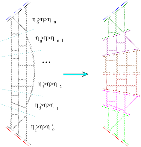
Figure 35: Effective action factorized in $n$ functional integrals.

The effective action factorizes then into a product of $n$ independent functional integrals over the gluon fields labeled by index $k$:

$$e^{iS_{\rm eff}(U,V;\eta)} = \int\!DA_{1}\ldots DA_{n+1}\ \exp i\Big{\{}V_{i}Y_{n+1}^{i}+S(A_{n+1})$$

$$+ W_{n+1,i}Y_{n}^{i}+S(A_{n})+\ldots+W_{2i}Y^{i}_{1}+S(A_{1})+W_{1}^{i}U_{i}\Big{\}},$$

where the integrals over $x_{\perp}$ and summation over the color indices are implied. As usual, $Y^{i}_{k}={i\over g}Y^{\dagger}_{k}\partial^{i}Y_{k}$ and $W^{i}_{k}={i\over g}W^{\dagger}_{k}\partial^{i}W_{k}$ where

$$Y_{k}(x_{\perp}) = P\ \exp ig\int_{-\infty}^{\infty}du\ n_{k}^{\mu}A_{k,\mu}(un^{k}+x_{\perp}),$$

$$W_{k}(x_{\perp}) = P\ \exp ig\int_{\infty}^{\infty}du\ n_{k-1}^{\mu}A_{k,\mu}(un^{k-1}+x_{\perp}),$$ (231)

and the vectors $n_{k}$ are ordered in rapidity: $\eta_{0}>\eta_{n}>\eta_{n-1}\ldots\eta_{2}>\eta_{1}>\eta^{\prime}_{0}$. To disentangle integrations over different $A^{k}$ we use the formula

$$e^{i\int dx_{\perp}W_{i}Y^{i}} = \det(\partial_{i}-igW_{i})(\partial^{i}-igY^{i})$$

$$\times \int DV(x_{\perp})DU(x_{\perp})e^{i\int dx_{\perp}W_{i}U^{i}+i\int dx_{\perp}V_{i}Y^{i}-i\int dx_{\perp}V_{i}U^{i}}.$$

The determinant gives the perturbative non-logarithmic corrections of the same order as the corrections to the factorization formula (4.1). In the LLA they can be ignored, consequently, we obtain

$$e^{iS_{\rm eff}(U,V)} = \int DA_{1}\ldots DA_{n+1}DU_{1}DV_{1}\ldots DU_{n}DV_{n}$$ (233)

$$\times \exp i\Big{\{}V_{i}Y_{n+1}^{i}+S(A_{n+1})+W_{n+1}^{i}U_{n,i}-V_{n,i}Y^{i}_{n}+\ldots$$

$$+ W_{3i}U^{i}_{2}-V_{2}^{i}U_{2i}+V_{2,i}Y^{i}_{2}+S(A_{2})+W_{2,i}U_{1}^{i}-V_{1,i}U_{1}^{i}$$

$$+ V_{1,i}Y^{i}_{1}+S(A_{1})+W_{1}^{i}U_{i}\Big{\}}.$$

Now we can integrate over the gluon fields $A_{k}$,

$$\int DA_{k}e^{V_{k,i}Y_{k}^{i}+S(A_{k})+W_{k,i}U^{i}_{k-1}}=e^{iS_{\rm eff}(V^{k},U^{k-1};\Delta\eta)}~{};$$ (234)

at sufficiently small $\Delta\eta$

$$S_{\rm eff}(V^{k},U^{k-1};\Delta\eta)=V_{k,i}U_{k-1}^{i}-i\Delta\eta K(V_{k},U_{k-1})+O(\Delta\eta^{2}),$$ (235)

where K is the kernel calculated in the previous section,

$$K(V,U) = -\alpha_{s}\int d^{2}x_{\perp}$$ (236)

$$\times \Bigg{\{}L_{1}^{a}{1\over\vec{\partial}_{\perp}^{2}}L_{1}^{a}+L_{2}^{a}\big{(}U^{\dagger}{1\over\vec{\partial}_{\perp}^{2}}U+V^{\dagger}{1\over\vec{\partial}_{\perp}^{2}}V-{1\over\vec{\partial}_{\perp}^{2}}\big{)}^{ab}L_{2}^{b}$$

$$+ L_{1}^{a}\big{(}{\partial_{i}\over\vec{\partial}_{\perp}^{2}}U^{\dagger}{\partial_{k}\over\vec{\partial}_{\perp}^{2}}U-U\leftrightarrow V\big{)}L^{b}_{2}\epsilon^{ik}$$

$$- L_{2}^{a}\epsilon^{ik}\big{(}U^{\dagger}{\partial_{i}\over\vec{\partial}_{\perp}^{2}}U{\partial_{k}\over\vec{\partial}_{\perp}^{2}}-U\leftrightarrow V\big{)}^{ab}L^{b}_{1}$$

$$+ {i\over 4\pi}\Big{(}V_{i}\big{(}U^{\dagger}(\ln\vec{\partial}_{\perp}^{2})U+V^{\dagger}(\ln\vec{\partial}_{\perp}^{2})V-(\ln\vec{\partial}_{\perp}^{2})\big{)}U^{i}\Big{)}^{aa}\Bigg{\}}.$$

Performing the integrations over $A^{k}$ we get

$$e^{iS_{\rm eff}(U,V)} = \int DV_{1}DU_{1}\ldots DV_{n}DU_{n}\ \exp\Big{\{}iV_{i}U^{i}_{n}+K(V,U_{n})\Delta\eta$$

$$- iV_{n,i}U^{i}_{n}+iV_{n,i}U_{n-1}^{i}+K(V_{n},U_{n-1})\Delta\eta+\ldots-iV_{2i}U^{i}_{2}$$

$$- iV_{2}^{i}U_{1i}+K(V_{2},U_{1})\Delta\eta-iV_{1}^{i}U_{1i}+iV_{1}^{i}U_{i}+K(V_{1},U)\Delta\eta\Big{\}}.$$

In the limit $n\rightarrow\infty$ we obtain the following functional integral for the effective action

$$e^{iS_{\rm eff}(U,V)} = \left.\int DV(\eta)DU(\eta)\right|_{U(\eta_{0}^{\prime})=U}~{}\exp\Big{\{}iV^{a}_{i}U^{ai}(\eta)$$

$$+ \int_{\eta^{\prime}_{0}}^{\eta_{0}}d\eta\Big{(}-iV^{ai}(\eta)\dot{U}^{a}_{i}(\eta)+K(V(\eta),U(\eta)\Big{)}\Big{\}}.$$

where we displayed the color indices explicitly. This looks like the functional integral over the canonical coordinates $U$ and canonical momenta $V$ with the (non-local) Hamiltonian $K(V,U)$. The rapidity $\eta$ serves as the time variable for this system. Let us demonstrate that perturbative expansion for the functional integral (5.2) determines the effective field theory for reggeized gluons. To get the perturbative series for the functional integral (5.2), we write down $U(\eta)$ and $V(\eta)$ as

$$U(x_{\perp},\eta)=e^{-ig\phi(x_{\perp},\eta)},\qquad\qquad V(x_{\perp},\eta)=e^{-ig\pi(x_{\perp},\eta)},$$ (239)

($\phi^{a}(x_{\perp},\eta)$ and $\pi^{a}(x_{\perp},\eta)$ are scalar fields) and expand in powers of $g$. In the leading order in $g$ we obtain

$$e^{iS_{\rm eff}(\phi,\pi)} = \left.\int D\pi(\eta)D\phi(\eta)\right|_{\phi(\eta^{\prime}_{0})=\phi}~{}\exp\Bigg{\{}-i\partial_{i}\pi^{a}\partial_{i}\phi^{a}(\eta_{0})$$ (240)

$$+ 2{\rm Tr}\int_{\eta^{\prime}_{0}}^{\eta_{0}}d\eta\Big{(}i\partial_{i}\pi(\eta)\left({\partial\over\partial\eta}+{\alpha_{s}\over 4\pi}N_{c}\ln\vec{\partial}_{\perp}^{2}\right)\partial_{i}\phi(\eta)$$

$$- \alpha_{s}[\bar{\partial}\pi(\eta),\tilde{\partial}\phi(\eta)]{1\over\vec{\partial}_{\perp}^{2}}[\tilde{\partial}\pi(\eta),\bar{\partial}\phi(\eta)]\Big{)}\Bigg{\}},$$

where $\tilde{\partial}\equiv\partial_{1}+i\partial_{2}$, $\bar{\partial}\equiv\partial_{1}-i\partial_{2}$. The bare propagator for these fields is (cf. Ref. 2)

$$\langle\phi(x_{\perp},\eta)~{}\phi(y_{\perp},\eta^{\prime})\rangle=0,\qquad\qquad\langle\pi(x_{\perp},\eta)~{}\pi(y_{\perp},\eta^{\prime})\rangle=0,$$

$$\langle\phi(x_{\perp},\eta)~{}\pi(y_{\perp},\eta^{\prime})\rangle=\theta(\eta-\eta^{\prime})\hbox{\bf\Big{(}$\!\!$\Big{(}}x_{\perp}\Big{|}{i\over\vec{p}_{\perp}^{2}}\Big{|}y_{\perp}\hbox{\bf\Big{)}$\!\!$\Big{)}}.$$ (241)

The $\theta$ function in this formula satisfies the condition $\theta(0)=0$ as can be easily seen from the limiting formula (5.2). It is convenient to include the $g^{2}\pi\vec{\partial}_{\perp}^{2}\ln\vec{\partial}_{\perp}^{2}\phi$ in the kinetic term rather than in the interaction Hamiltonian. Since this expression is IR divergent one should at first consider the regularized $S_{\rm eff}$

$$e^{iS_{\rm eff}(\phi,\pi)} = \int D\phi D\pi\exp\Bigg{\{}2{\rm Tr}\int_{\eta^{\prime}_{0}}^{\eta_{0}}d\eta\Big{\{}i\partial_{i}\pi\left({\partial\over\partial\eta}+{\alpha_{s}\over 4\pi}N_{c}\ln{\vec{\partial}_{\perp}^{2}\over\mu^{2}}\right)\partial_{i}\phi$$ (242)

$$- \alpha_{s}[\partial\phi,\bar{\partial}\pi]{1\over\vec{\partial}_{\perp}^{2}+\mu^{2}}[\partial\phi,\bar{\partial}\pi]\Big{\}}-i\partial_{i}\pi^{a}\partial_{i}\phi^{a}(\eta_{0})\Bigg{\}}$$

and then take the limit $\mu^{2}\rightarrow 0$. (Alternatively, one can use the regularization $d=2+\epsilon$ for the number of transverse dimensions as it was done in Sec. 5.1.) The propagator takes the form

$$\langle\phi(x_{\perp},\eta)~{}\phi(y_{\perp},\eta^{\prime})\rangle=0,\qquad\qquad\langle\pi(x_{\perp},\eta)~{}\pi(y_{\perp},\eta^{\prime})\rangle=0,$$ (243)

$$\int{dp_{\perp}\over 4\pi^{2}}e^{ip(x-y)_{\perp}}\langle\phi(x_{\perp},\eta)\pi(y_{\perp},\eta^{\prime})\rangle=\theta(\eta-\eta^{\prime}){i\over\vec{p}_{\perp}^{2}}e^{-{\alpha_{s}\over 4\pi}N_{c}(\eta-\eta^{\prime})\ln{p^{2}\over\mu^{2}}},$$

which coincides with the propagator of the reggeized gluon (73).

Since the only non-vanishing Green functions are

$$\langle\phi(x_{1},\eta)\ldots\phi(x_{m},\eta)\pi(y_{1},\eta^{\prime})\ldots\pi(y_{n},\eta^{\prime})\rangle$$

with $m=n$, the number of reggeized gluons is conserved. It is easy to see that the Feynman rules for the Green function

$$\langle\phi(x_{1},\eta)\ldots\phi(x_{n},\eta)\pi(y_{1},\eta^{\prime})\ldots\pi(y_{n},\eta^{\prime})\rangle$$

reproduce the diagrams for the quantum mechanics of $n$ particles with Lipatov’s Hamiltonian (2.5) (see Fig. 10).

In the next order in the expansion (239) we get

$$e^{iS_{\rm eff}(\phi,\pi)} = \left.\int D\pi(\eta)D\phi(\eta)\right|_{\phi(\eta^{\prime}_{0})=\phi}~{}\exp\Bigg{\{}-i\partial_{i}\pi^{a}\partial_{i}\phi^{a}(\eta_{0})$$

$$+ 2{\rm Tr}\int_{\eta^{\prime}_{0}}^{\eta_{0}}\Big{\{}i\partial_{i}\pi(\eta)\left({\partial\over\partial\eta}+{\alpha_{s}\over 4\pi}N_{c}\ln\vec{\partial}_{\perp}^{2}\right)\partial_{i}\phi(\eta)$$

$$- \alpha_{s}[\partial\phi,\bar{\partial}\pi]{1\over\vec{\partial}_{\perp}^{2}}[\partial\phi,\bar{\partial}\pi]\Big{\}}+i{g^{3}\over 4\pi}K_{(3)}(\phi,\pi)+{g^{4}\over 4\pi}K_{(4)}(\phi,\pi)\Bigg{\}},$$

where

$$K_{(3)}(\phi,\pi) = \Bigg{\{}\big{[}[\partial_{i}\phi,\phi],\partial_{i}\pi\big{]}{1\over\vec{\partial}_{\perp}^{2}}[\partial_{j}\phi,\partial_{j}\pi]$$

$$+ \Big{(}\big{[}[\partial_{i}\phi,\phi],\partial_{j}\pi\big{]}+2\big{[}\phi,[\partial_{i}\phi,\partial_{j}\pi\big{]}\Big{)}{1\over\vec{\partial}_{\perp}^{2}}\big{(}[\partial_{i}\phi,\partial_{j}\pi]-(i\leftrightarrow j)\big{)}$$

$$- 2[\partial_{j}\phi,\partial_{j}\pi]{\partial_{i}\over\vec{\partial}_{\perp}^{2}}\phi^{a}{\partial_{k}\over\vec{\partial}_{\perp}^{2}}\big{(}\big{[}t^{a},[\partial_{i}\phi,\partial_{k}\pi]\big{]}-(i\leftrightarrow k)\big{)}\Bigg{\}}+\Big{\{}\pi\leftrightarrow\phi\Big{\}}$$

and

$$K_{(4)}(\phi,\pi) = \big{[}[\partial_{i}\phi,\phi],[\partial_{i}\pi,\pi]\big{]}{1\over\vec{\partial}_{\perp}^{2}}[\partial\phi,\bar{\partial}\pi]$$

$$+ \big{[}[\partial\phi,\phi],\partial_{i}\pi\big{]}{1\over\vec{\partial}_{\perp}^{2}}\big{[}[\partial_{i}\phi,\phi],\partial_{i}\pi\big{]}+\ldots.$$

The number of reggeized gluons is no longer conserved, hence we get the field theory of reggeized gluons with Feynman diagrams shown in Fig. 36.

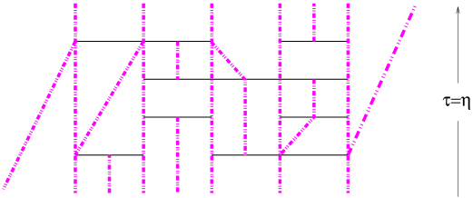
Figure 36: Feynman diagrams for the field theory of reggeized gluons.

In higher orders we will get more complicated $\pi^{m}\phi^{n}$ vertices.

It is intersting to compare (233) with Lipatov’s effective action for reggeized gluons.[22, 2] In these papers the reggeon is defined as a scalar field depending on both transverse and longitudinal coordinates. The integration of Lipatov’s effective action over longitudinal coordinates of the reggeons in the LLA reproduces the first two (BFKL and three-pomeron) terms in the expansion (233). Hopefully, the integration of the Lipatov’s action in the NLO LLA, NNLO LLA etc. will reproduce the expansion (233) order by order in perturbation theory.

5.3 Semiclassical approach to Wilson-line functional integral for the effective action

Perturbation expansion (239) is relevant when the characteristic $U_{i}$ and $V_{i}$ inside the functional integral (5.2) are $\sim O(1)$. However, we shall see below that at high energies the characteristic fields in this functional integral seem to be large, consequently the expansion (239) may be useless. In this case, we can try to calculate the functional integral (5.2) semiclassically. The classical equations for the functional integral (5.2) are

$$(i\partial_{i}+g[V_{i})\dot{U}^{i} = -{\delta\over V^{\dagger}\delta V}K(U,V),$$

$$(i\partial_{i}+g[U_{i})\dot{V}^{i} = {\delta\over U^{\dagger}\delta U}K(U,V),$$ (247)

with the initial conditions

$$U(\eta)=U~{}{\rm at}~{}\eta=\eta^{\prime}_{0},\qquad\qquad V(\eta)=V~{}{\rm at}~{}\eta=\eta_{0}.$$ (248)

Let us denote the solution of these equation by $\bar{U}(x_{\perp},\eta)$ and $\bar{V}(x_{\perp},\eta)$. In the LLA the semiclassical calculation of the Wilson-line integral (5.2) is equivalent to the semiclassical calculation of the original functional integral (191). I will make a conjecture that the saddle point of the original functional integral (200), satisfying the classical equations (206), corresponds to the classical solution (4.1) of the Wilson-line integral (5.2) even beyond the LLA:

$$\exp\left\{iV_{i}\bar{Y}^{i}(\eta_{0})+i\bar{W}_{i}(\eta^{\prime}_{0})U^{i}+iS(\bar{A})\right\}$$

$$= \exp\Bigg{\{}iV_{i}\bar{U}_{i}(\eta_{0})+\int_{\eta^{\prime}_{0}}^{\eta_{0}}d\eta\Big{(}-i\bar{V}^{i}(\eta)\dot{\bar{U}}_{i}(\eta)+K(\bar{V}(\eta),\bar{U}(\eta)\Big{)}\Bigg{\}},$$

where $\bar{A}$ is the classical solution of the equations (206). (As in previous section, we do not display the integrals over the transverse coordinates). Being a quantum correction, the gluon reggeization (5.1) exceeds the accuracy of the semiclassical approximation, hence we can drop the last (reggeization) term in the kernel (236).

Talking the variational derivative of both sides of Eq. (5.3) with respect to $V$, we obtain

$$\bar{Y}_{i}(\eta)=\bar{U}_{i}(\eta).$$ (250)

If we now take the derivative of both sides with respect to $\eta_{0}$, we get the equation

$$iV_{i}\dot{\bar{Y}}_{i}(\eta_{0})=iV_{i}\dot{\bar{U}}_{i}(\eta_{0})=K(V,\bar{U}(\eta_{0})),$$ (251)

which may be used for the calculation of $K$. Correspondingly, one can differentiate with respect to $\eta^{\prime}_{0}$ resulting in

$$-i\dot{\bar{V}}_{i}(\eta^{\prime}_{0})U_{i}=K(\bar{V}(\eta^{\prime}_{0}),U).$$ (252)

Since $V$ in Eq. (251) and $U$ in Eq. (252) are arbitrary, we may substitute $\bar{V}(\eta)$ and $\bar{U}(\eta)$ instead :

$$i\bar{V}_{i}(\eta)\dot{\bar{U}}_{i}(\eta)=-i\dot{\bar{V}}_{i}(\eta)\bar{U}_{i}(\eta)=K(\bar{V}(\eta),\bar{U}(\eta)).$$ (253)

The exponential of the Wilson-line functional integral vanishes except for the non-integral term $V_{i}\bar{U}^{i}(\eta_{0})=V_{i}\bar{Y}^{i}(\eta_{0})$, so

$$\exp\left\{iV_{i}\bar{Y}^{i}(\eta^{\prime}_{0})+i\bar{W}_{i}(\eta_{0})U^{i}+iS(\bar{A})\right\} = \exp\big{\{}iV_{i}\bar{U}_{i}(\eta_{0})\big{\}}$$ (254)

$$= \exp\big{\{}i\bar{V}_{i}(\eta^{\prime}_{0})U_{i}\big{\}}.$$

Thus, in a semiclassical approximation (and with the assumption mentioned above) we obtain

$$S_{\rm eff}=V_{i}\bar{U}_{i}(\eta_{0})=\bar{V}_{i}(\eta^{\prime}_{0})U_{i}=-S(\bar{A}),$$ (255)

so that all the three terms in left-hand side of Eq. (5.3) contribute equally up to a different sign for $S(\bar{A})$. We have checked it in LLA and it is crucial to check it in the next-to-leading order. From Eqs. (253) and (255) we see that the effective action in the semiclassical approximation can be written down also as

$$S_{\rm eff}=\bar{V}_{i}(\eta)\bar{U}_{i}(\eta)$$ (256)

for arbitrary $\eta$.

Instead of taking variational derivatives of the kernel $K(V,U)$, it is possible to calculate $\dot{\bar{U}}\equiv\dot{\bar{Y}}$ directly. One obtains (cf. Eq. (216))

$$\![x_{\perp},-\infty p_{1}+x_{\perp}]^{(1)} = {ig^{2}\over 2\pi}\ln{\sigma\over\sigma^{\prime}}\int d^{2}z_{\perp}$$

$$\times \hbox{\bf\Big{(}$\!\!$\Big{(}}x_{\perp}\Big{|}{1\over\vec{p}_{\perp}^{2}}\Big{|}z\hbox{\bf\Big{)}$\!\!$\Big{)}}\Big{(}L_{1}(z_{\perp})+2[U_{i}(z_{\perp}),\Delta^{i}(z_{\perp})]\Big{)},$$

$$\![\infty p_{1}+x_{\perp},x_{\perp}]^{(1)} = -{ig^{2}\over 2\pi}\ln{\sigma\over\sigma^{\prime}}t^{a}\int d^{2}z_{\perp}$$

$$\times \hbox{\bf\Big{(}$\!\!$\Big{(}}x_{\perp}\Big{|}U^{\dagger}{1\over\vec{p}_{\perp}^{2}}U+U^{\dagger}{1\over\vec{p}_{\perp}^{2}}(\vec{\partial}^{2}_{\perp}U){1\over\vec{p}_{\perp}^{2}}\Big{|}z\hbox{\bf\Big{)}$\!\!$\Big{)}}^{ab}L^{b}_{1}(z_{\perp}),$$

and, therefore,

$$[\infty p_{1}+x_{\perp},-\infty p_{1}+x_{\perp}]^{(1)}~{}=~{}{ig^{2}\over\pi}\ln{\sigma\over\sigma^{\prime}}\int d^{2}z_{\perp}$$

$$\times~{}\Bigg{\{}\hbox{\bf\Big{(}$\!\!$\Big{(}}x_{\perp}\Big{|}{1\over\vec{p}_{\perp}^{2}}\Big{|}z_{\perp}\hbox{\bf\Big{)}$\!\!$\Big{)}}[U_{i}(z_{\perp}),\Delta^{i}(z_{\perp})]-t^{a}\hbox{\bf\Big{(}$\!\!$\Big{(}}x_{\perp}\Big{|}U^{\dagger}{p^{k}\over\vec{p}_{\perp}^{2}}i(\partial_{k}U){1\over\vec{p}_{\perp}^{2}}\Big{|}z_{\perp}\hbox{\bf\Big{)}$\!\!$\Big{)}}^{ab}L^{b}_{1}(z_{\perp})\Bigg{\}}$$

$$=~{}{ig^{2}\over\pi}t^{a}\ln{\sigma\over\sigma^{\prime}}\int d^{2}z_{\perp}\Bigg{\{}\hbox{\bf\Big{(}$\!\!$\Big{(}}x_{\perp}\Big{|}-U^{\dagger}{p^{k}\over\vec{p}_{\perp}^{2}}i(\partial_{k}U){1\over\vec{p}_{\perp}^{2}}\Big{|}z_{\perp}\hbox{\bf\Big{)}$\!\!$\Big{)}}^{ab}L^{b}_{1}(z_{\perp})$$

$$\hskip 85.35826pt+~{}\hbox{\bf\Big{(}$\!\!$\Big{(}}x_{\perp}\Big{|}{p_{i}\over\vec{p}_{\perp}^{2}}U^{\dagger}{p_{k}\over\vec{p}_{\perp}^{2}}U\Big{|}z\hbox{\bf\Big{)}$\!\!$\Big{)}}^{ab}\epsilon^{ik}L^{b}_{2}(z_{\perp})\Bigg{\}}.$$ (258)

The derivative $\bar{U}^{\dagger}\dot{\bar{U}}$ is half of the coefficient in front of $\ln{\sigma\over\sigma^{\prime}}$ in this formula so we obtain

$$\bar{U}^{\dagger}\dot{\bar{U}}={ig^{2}\over 2\pi}\left(\bar{U}^{\dagger}{\partial^{k}\over\vec{\partial}_{\perp}^{2}}(\partial_{k}\bar{U})\right)^{ab}{1\over\vec{\partial}_{\perp}^{2}}\bar{L}^{b}_{1}-{ig^{2}\over 2\pi}{\partial_{i}\over\vec{\partial}_{\perp}^{2}}\left(\bar{U}^{\dagger}{\partial_{k}\over\vec{\partial}_{\perp}^{2}}\bar{U}\right)^{ab}\epsilon^{ik}\bar{L}^{b}_{2},$$ (259)

and, similarly,

$$\bar{V}^{\dagger}\dot{\bar{V}}=-{ig^{2}\over 2\pi}\left(\bar{V}^{\dagger}{\partial^{k}\over\vec{\partial}_{\perp}^{2}}(\partial_{k}\bar{V})\right)^{ab}{1\over\vec{\partial}_{\perp}^{2}}\bar{L}^{b}_{1}-{ig^{2}\over 2\pi}{\partial_{i}\over\vec{\partial}_{\perp}^{2}}\left(\bar{V}^{\dagger}{\partial_{k}\over\vec{\partial}_{\perp}^{2}}\bar{V}\right)^{ab}\epsilon^{ik}\bar{L}^{b}_{2},$$ (260)

where $\bar{U}\equiv{\bar{U}}(\eta),~{}\bar{V}\equiv{\bar{V}}(\eta)$.

For illustration, let us present a first few terms in the semiclassical expansion of the effective action,

$$\bar{S}_{\rm eff} = \int d^{2}x_{\perp}V_{i}U^{i}$$

$$+ {ig^{2}\over 2\pi}\ln{\sigma\over\sigma^{\prime}}\int d^{2}x_{\perp}\Big{(}L_{1}^{a}{1\over\vec{\partial}_{\perp}^{2}}L_{1}^{a}-{1\over g^{2}}\Delta^{a}_{i}\Delta^{a,i}+2L_{1}^{a}{1\over\vec{\partial}_{\perp}^{2}}\big{(}U_{i}-V_{i}\big{)}^{ab}\Delta^{b,i}$$

$$+ {1\over 2}\left({g^{2}\over 2\pi}\ln{\sigma\over\sigma^{\prime}}\right)^{2}\Big{\{}L_{1}^{a}\Big{(}{1\over\vec{\partial}_{\perp}^{2}}(\partial^{k}U^{\dagger}){\partial_{k}\over\vec{\partial}_{\perp}^{2}}U\Big{)}^{ab}-\Delta^{ak}U_{k}^{ab}{1\over\vec{\partial}_{\perp}^{2}}\Big{\}}$$

$$\times \Big{(}(\partial^{i}-igU^{i})(\partial_{i}-igV_{i})\Big{)}^{bc}\Big{\{}\Big{(}V^{\dagger}{\partial_{j}\over\vec{\partial}_{\perp}^{2}}(\partial^{j}V){1\over\vec{\partial}_{\perp}^{2}}\Big{)}^{cd}L_{1}^{d}+{1\over\vec{\partial}_{\perp}^{2}}V_{j}^{cd}\Delta^{dj}\Big{\}}.$$

Once we know the solution of the Wilson-line classical equations (259)-(260), it is possible to restore $\bar{A}$. Suppose we want to find $\bar{A}(\eta_{x},\tau,x_{\perp})$ where $\tau=x_{\parallel}^{2}$ and $\eta_{x}=\ln{x_{*}\over x_{\bullet}}$. Let us insert two factorization formulas at $\eta_{x}+\delta\eta$ and $\eta_{x}-\delta\eta$ and integrate over the fields in the regions $\eta_{0}>\eta_{x}+\delta\eta$ and $\eta_{x}-\delta\eta>\eta>\eta^{\prime}_{0}$ semiclassically. The final integration over the region of rapidities $\eta+\delta\eta>\eta>\eta_{x}-\delta\eta$ takes the form

$$\int\!\!\!D\!A\ \exp\left\{i\bar{V}^{i}(\eta_{x}+\Delta\eta)Y_{i}(\eta_{x}+\Delta\eta)+iW^{i}(\eta_{x}-\Delta\eta)\bar{U}_{i}(\eta_{x}-\Delta\eta)+iS(A)\right\}.$$ (262)

(Here $\eta_{x}+\Delta\eta$ denotes the argument for the classical solution $\bar{V}^{i}$ and the direction of the Wilson line for $Y_{i}$). Comparing this to Eq. (200), we find that the field $\bar{A}(\eta_{x},\tau,x_{\perp})$ is given by expressions (210) with $U\rightarrow\bar{U}(\eta)$, $V\rightarrow\bar{V}(\eta)$. Unfortunately, the accuracy is again up to $[\bar{U}(\eta),\bar{V}(\eta)]^{2}$. Still, we see that the fields contain logarithms of $\eta_{x}$ coming from and $\bar{U}(\eta)$ $\bar{V}(\eta)$ so our assumption about large characteristic fields in the functional integral (191) is justified. Note that for the infinite Wilson line in $\eta_{x}$ direction we can get an (almost) explicit expression in terms of $U\rightarrow\bar{U}(\eta)$ and $V\rightarrow\bar{V}(\eta)$ without the restriction $[\bar{U}(\eta),\bar{V}(\eta)]\ll 1$. It is easy to see that

$$[x_{\perp}-\infty n_{\eta},x_{\perp}+\infty n_{\eta}](i\partial_{i}+\bar{A}_{i}(x_{\perp}+\infty n_{\eta}))[x_{\perp}+\infty n_{\eta},x_{\perp}-\infty n_{\eta}]=\Lambda_{i}(x_{\perp},\eta),$$ (263)

where $\Lambda_{i}(x_{\perp},\eta)=\bar{U}(x_{\perp},\eta)+\bar{V}(x_{\perp},\eta)+\bar{\Delta}(x_{\perp},\eta)$ is pure gauge field satisfying the equation

$$\left(i\partial_{i}+[\bar{U}_{i}+\bar{V}_{i},\right)\Delta_{i}=0,$$ (264)

(see Eq. (5.1). Indeed, let us try to calculate the l.h.s. of the Eq. (263). At small $\delta\eta$ all the contributions coming from $[x_{\perp}+\infty n_{\eta},x_{\perp}-\infty n_{\eta}]$ contain $\delta\eta$ (see Eq. (25)), hence they are small. The only non-vanishing contribution comes from $\bar{A}_{i}(x_{\perp}+\infty n_{\eta})$ which coincide with $\Lambda_{i}(x_{\perp},\eta)$ in the background-Feynman gauge (264).

6 Conclusions and outlook

First I would like to discuss the relation of this method to other approaches to the high-energy QCD discussed in the literature.

By far, the most popular approach to high-energy pQCD is the direct summation of Feynman diagrams (and related methods based on unitarity relations in $s$ and $t$ channels). Although the majority of the results in pQCD, including the NLO BFKL kernel, were obtained by this method, I think that even in pQCD, the Wilson-line language, combined with the calculation of the propagators in the shock-wave background, is technically more powerful. (Perhaps the comparison of the diagrammatic calculation of the three-pomeron vertex in Ref. 45 to the computation of the gluon propagator in the shock-wave background in Sec. 7.3 demonstrates this most clearly).

The dipole picture [57] has an advantage of visual interpretation of the high-energy scattering, especially in the case of DIS at small $x$.[24, 25] The dipole language is a light-cone version of the Wilson-line approach combined with large-$N_{c}$ approximation for the wave functions at small $x$. However, it is hard to think about the effective action in terms of the dipoles, since in order to study the energy evolution of the effective action we must take into account not only the creation of the new dipoles, but their multiple creation and recombination, which is difficult to define in the framework of the dipole model.

The most close in spirit to our semiclassical method is the renormalization-group approach to the high-energy scattering from the large nuclei advocated in the papers of L. McLerran and collaborators (see e.g. Refs. 4, 52, 58). In this approach, the small-x evolution of one strong shock wave (created by a source $\rho(x_{\perp})$) is studied in the light-like gauge. With such a choice of gauge, the second shock wave can be treated perturbatively at the very end of the evolution process. In our terms, this amounts to the solution of classical Eqs. (206) using the trial configuration $A_{i}=U_{i}\theta(x_{\ast})$ (instead of starting point $A_{i}=U_{i}\theta(x_{\ast})+V_{i}\theta(x_{\bullet})+\Delta_{i}$ taken in this paper). Unfortunately, due to different gauges adopted in our paper and Refs. 52, 58, the treatment of the boundary terms in the functional integral is different, leading to the different sources for the shock waves and making hard to compare the intermediate formulas. However, since the first-order (BFKL) results coincide I think these effective actions are essentially the same.

In conclusion I would like to outline possible uses of this approach. The ultimate goal is to obtain the explicit expression for the effective action in all orders in $\ln{s\over m^{2}}$. One possible prospect is that due to the conformal invariance of QCD at the tree level our future result for the effective action can be formalized in terms of conformal two-dimensional theory in external two-dimensional “gauge fields” $V_{i}$ and $U_{i}$. So far, I was not able to use the conformal invariance because it is not obvious how to implement it in terms of Wilson-line operators. We can, however, expand Wilson lines back to gluons. The conformal properties of (reggeized) gluon amplitudes are now well studied. In the coordinate space the BFKL kernel is invariant under Mobius group and therefore the eigenfunctions of BFKL kernel are simply powers of coordinates. It is not clear which part of the conformal symmetry survives for the full effective action, yet there is every reason to believe that it will simplify the structure of the answer even after reassembling of Wilson lines.

The semiclassical approach developed above for the small-x processes in perturbative QCD can be applied for studying the heavy-ion collisions. As advocated in Ref. 4, the coupling constant for the heavy-ion collisions may be relatively small due to high density. An estimation of the corresponding “parton saturation scale” $Q_{s}$ gives $\sim 1$ GeV for RHIC and $\sim 2-3$ GeV for LHC,[7] so $g(Q_{s})$ is a valid perturbative parameter. On the other hand, the fields produced by colliding ions are large, so that the product $gA$ is not small, showing that the Wilson-line gauge factors $V$ and $U$ are of order of 1. Thus, we have a perfect situation to try sQCD methods.

It should however be mentioned that in this paper we considered the special case of the collision of the two shock waves, namely without any particles in the final state. It follows from the usual boundary conditions for Feynman amplitude (81) which we calculate: no outgoing waves at $t\rightarrow\infty$ and no incoming fields at $t\rightarrow-\infty$ (the latter condition is satisfied automatically by the $\left.A\right|_{t\rightarrow-\infty}=0$ choice of gauge). However, people are usually interested in the process of particle production during the collision (see e.g. Ref. 59) since it gives the experimental probe of quark-gluon plasma. In this case, our approach must be modified for the new boundary conditions — we must solve the classical equations (206) with Feynman boundary conditions only at $t\rightarrow-\infty$. The boundary condition at $t\rightarrow\infty$ depends on the problem under investigation: in the case if we are interested in the the total cross section (cut diagrams) we must calculate the double functional integral corresponding to the integration over the “+” fields to the right and the “–” fields to the left of the cut (see Ref. 43). (This is actually a functional-integral formalization of Cutkosky rules). In this case we may use the usual (Feynman and c.c. Feynman) propagators for each type of the fields. The boundary condition requires that two types of the field — the left-side “–” fields and the right-side “+” ones — coincide at $t\rightarrow\infty$. (This boundary condition is responsible for the $\delta(p^{2})\theta(p_{0})$ propagators on the cut). Finally, to find the total cross section of the shock-wave collision in the semiclassical approximation, we must solve the double set of classical equations for “+” and “–” fields with the boundary condition that these fields coincide at infinity (cf. Ref. 60). The study is in progress.

7 Appendix

7.1 Wilson lines from Feynman diagrams

Let us demonstrate that the relevant operators are Wilson lines (3). The typical contribution to the Green function of the fast-moving quark (with $\alpha_{k}\ll\sigma$) is shown in Fig. 37

Figure 37: Typical diagram for the propagator of fast-moving quark.

where the gluons have $\alpha\ll\sigma$. Consider the loop integral over $p$. Since we can neglect $\alpha_{p}$ as compared to $\alpha_{k}$, the quark propagator with the momentum $k-p$ reduces to

$$\not\!p_{2}\frac{\not\!k-\not\!p}{(k-p)^{2}+i\epsilon}\not\!p_{2}\rightarrow\frac{\not\!p_{2}}{\beta_{k}-\beta_{p}-{(\vec{k}-\vec{p})_{\perp}^{2}\over\alpha_{k}s}+i\epsilon\alpha_{k}}.$$ (265)

Here we have used the fact that $g_{\mu\nu}$ in the numerator of the gluon propagator connecting the lines with very different rapidities ($\equiv\alpha$’s) can be replaced by $\frac{2}{s}p_{1\mu}p_{2\nu}$.

I will prove now that if I replace the propagator (265) by

$${\not\!p_{2}\over-\beta_{p}+i\epsilon\alpha_{k}},$$ (266)

the value of the loop integral over $p$ remains unchanged. Indeed, the integral over $p$ is the sum of the residue in the pole corresponding to the fast-quark propagator (265) and/or the residues in the slow-gluon propagators. Let us consider both residues in turn and verify that the replacement (266) does not affect the residues.

First, if I take the residue in the pole

$$\beta_{p}=\beta_{k}-\frac{(\vec{k}-\vec{p})_{\perp}^{2}}{\alpha_{k}s}$$ (267)

corresponding tho the quark propagator, the typical slow-gluon denominator takes the form

$$(\alpha_{p}+\tilde{\alpha_{p}})(\beta_{p}+\tilde{\beta_{p}})s-(p+\tilde{p})_{\perp}^{2}$$

$$= (\alpha_{p}+\tilde{\alpha_{p}})\beta_{p}s-(p+\tilde{p})_{\perp}^{2}+(\alpha_{p}+\tilde{\alpha_{p}})\beta_{k}s-{\alpha_{p}+\tilde{\alpha_{p}}\over\alpha_{k}}(\vec{k}-\vec{p})_{\perp}^{2}.$$

The first two terms are or order of $m^{2}$ while the second two ones are $\sim{\alpha_{p}\over\alpha_{k}}m^{2}$ and hence they can be neglected, which corresponds to taking the residue at the pole $\beta_{p}=0$ in the propagator (266). (Here we have used the fact that $\beta_{k}\sim{m^{2}\over\alpha_{k}s}$, see below).

Second possibility corresponds to the residue taken at

$$\beta_{p}=-\tilde{\beta}_{p}+{(p+\tilde{p})_{\perp}^{2}\over(\alpha_{p}+\tilde{\alpha_{p}})s}$$ (269)

in one of the slow-gluon propagators. The quark propagator (265) then takes the form

$$\frac{\not\!p_{2}}{\tilde{\beta_{p}}+{(p+\tilde{p})_{\perp}^{2}\over(\alpha_{p}+\tilde{\alpha_{p}})s}+\beta_{k}-{(\vec{k}-\vec{p})_{\perp}^{2}\over\alpha_{k}s}+i\epsilon\alpha_{k}}.$$ (270)

Again, the first two terms in the denominator are $\sim{m^{2}\over\alpha_{p}s}$, while the second two ones are $\sim{m^{2}\over\alpha_{p}s}\ll{m^{2}\over\alpha_{k}s}$ and can be neglected which is exactly equivalent to replacing the Eq. (265) by Eq. (266).

Hence, we have proved that the propagator of the fast quark can be reduced to (266) which is nothing but the eikonal gauge-factor in the momentum representation.

7.2 Quark propagator in a shock-wave background.

Let us now find the quark propagator in the shock-wave background. We start the path-integral representation of a quark Green function in the external field $B^{\Omega}$,

$${\hbox{\bf\Big{(}$\!\!$\Big{(}}}x\Big{|}\frac{1}{{\not\!{\cal P}}}\Big{|}y{\hbox{\bf\Big{)}$\!\!$\Big{)}}} = -i\int_{0}^{\infty}\!d\tau{\hbox{\bf\Big{(}$\!\!$\Big{(}}}x\Big{|}{\cal P}e^{i\tau{\cal P}^{2}}\Big{|}y{\hbox{\bf\Big{)}$\!\!$\Big{)}}}$$ (271)

$$= -i\int_{0}^{\infty}\!d\tau{\cal N}^{-1}\int_{x(0)=y}^{x(\tau)=x}\!{\cal D}x(t)\{{1\over 2}\not{\dot{x}}+\not\!{B^{\Omega}}(x(\tau))\}e^{-i\int_{0}^{\tau}\!dt{\dot{x}^{2}\over 4}}$$

$$\times P\ \exp\{ig\int_{0}^{\tau}\!dt(B^{\Omega}_{\mu}(x(t))\dot{x}^{\mu}(t)+{1\over 2}\sigma^{\mu\nu}G^{\Omega}_{\mu\nu}(x(t))\},$$

where $\sigma_{\mu\nu}\equiv{i\over 2}(\gamma_{\mu}\gamma_{\nu}-\gamma_{\nu}\gamma_{\mu})$. First, it is easy to see that since in our external field (90) the only nonzero components of the field tensor is $G^{\Omega}{\circ i}$ only the first two first term of the expansion of the exponent $\exp\{\int\!dt{i\over 2}(\sigma G^{\Omega})\}$ in powers of $(\sigma G)$ survive. Indeed, $\sigma^{\mu\nu}G^{\Omega}_{\mu\nu}={4i\over s_{0}}{\not\!p}^{0}_{2}\gamma^{i}G^{\Omega}_{{}_{\circ}i}$ and therefore $(\sigma G^{\Omega})^{2}\sim({\not\!p}_{2}\gamma^{i})^{2}=0$ since ${\not\!p}_{2}$ commutes with $\gamma^{i}_{\perp}$. Consequently, the phase factor for the motion of the particle in the external field (90) has the form

$$Pe^{ig\int_{0}^{\tau}\!dtB^{\Omega}_{\mu}(x(t))\dot{x}_{\mu}(t)}$$

$$+ {2\gamma^{i}{\not\!p}_{2}\over s}\int_{0}^{\tau}\!dt^{\prime}Pe^{ig\int_{t^{\prime}}^{\tau}\!dtB^{\Omega}_{\mu}(x(t))\dot{x}_{\mu}(t)}gG^{\Omega}_{\circ i}(x(t^{\prime}))Pe^{ig\int^{t^{\prime}}_{0}\!dtB^{\Omega}_{\mu}(x(t))\dot{x}_{\mu}(t)}.$$

Let us consider the case $x_{\ast}>0,y_{\ast}<0$ as shown in Fig. 13. Similarly to the case of scalar propagator, we can replace the gauge factor along the actual path $x_{\mu}(t)$ by the gauge factor along the straight-line path shown in Fig. 14 which intersects the plane $x_{\ast}=0$ at the same point $(z_{\circ},z_{\perp})$ at which the original path does. The gauge factor (273) reduces to

$$U^{\Omega}(z_{\perp})+{\gamma^{i}\!{\not\!p}_{2}\over\dot{x}_{\ast}(\tau^{\prime})}i\partial_{i}U^{\Omega}(z_{\perp})$$ (273)

where the last term was obtained using the identity

$$\frac{\partial}{\partial x_{i}}U(x_{\perp}) = -{2i\over s_{0}}\int\!dx_{\ast}[\infty p^{(0)}_{1},{2\over s_{0}}x_{*}p^{(0)}_{1}]_{x}G_{\circ i}({2\over s_{0}}x_{*}p^{(0)}_{1}+x_{\perp})$$ (274)

$$\times [{2\over s_{0}}x_{*}p^{(0)}_{1},-\infty p^{(0)}_{1}]_{x},$$

and the factor $\dot{x}_{\ast}(\tau^{\prime})$ in Eq. (7.2) comes from changing of variable of integration from $t$ to $x_{\ast}(t)$. Similarly, the phase factor for the term in the right-hand side of Eq. (271) which contains $\not\!B^{\Omega}(x(\tau))={2\over s_{0}}{\not\!p}_{2}B^{\Omega}_{\circ}(x(\tau))$ in front of the gauge factor Eq. (271) can be reduced to

$$-{\not\!p}_{2}{\partial\over\partial x_{*}}[{2\over s_{0}}x_{*}p^{(0)}_{1}+x_{\perp},-\infty+x_{\perp}]=-{\not\!p}_{2}\delta(x_{*})[U(x_{\perp})-1].$$ (275)

(The factor $\sim(\sigma G)$ is absent since it contains extra ${\not\!p}_{2}$ and ${\not\!p}_{2}^{2}=0$). If we now insert the expression for the phase factors (7.2), (275) into the path integral (271), we obtain (cf. Eq. (3.2))

$$- {\not\!p}_{2}\delta(x_{*})[U^{\Omega}(x_{\perp})-1]\int_{0}^{\infty}\!d\tau{\cal N}^{-1}\int^{x(\tau)=x}_{x(0)=y}\!{\cal D}x(t)e^{-i\int_{\tau}^{0}\!dt{\dot{x}^{2}\over 4}}$$

$$- {i\over 2}\int_{0}^{\infty}\!d\tau\int_{0}^{\tau}\!d\tau^{\prime}\int\!dz\delta(z_{*}){\cal N}^{-1}\int_{x(\tau^{\prime})=z}^{x(\tau)=x}\!{\cal D}x(t)\!\not{\dot{x}}(\tau)e^{-i\int_{\tau^{\prime}}^{\tau}\!dt{\dot{x}^{2}\over 4}}$$

$$\times \{U^{\Omega}(z_{\perp})+{i\over\dot{x}_{*}(\tau^{\prime})}\not{\partial}U^{\Omega}(z_{\perp}){\not\!p}_{2}\}{\cal N}^{-1}\int_{x(0)=y}^{x(\tau^{\prime})=z}\!{\cal D}x(t)\dot{x}_{*}(\tau^{\prime})e^{-i\int_{\tau^{\prime}}^{\tau}\!dt{\dot{x}^{2}\over 4}}.$$

Make a shift of time variable $\tau^{\prime}$ and using Eqs. (95) and (99) to perform path integrals in the right-hand side of Eq. (7.2), it is easy to reduce the path-integral expression for the quark propagator in the shock-wave field (91) to

$${\hbox{\bf\Big{(}$\!\!$\Big{(}}}x\Big{|}\frac{1}{{\not\!{\cal P}}}\Big{|}y{\hbox{\bf\Big{)}$\!\!$\Big{)}}} = \frac{{\not\!p}_{2}}{4\pi^{2}(x-y)^{2}}\delta(x_{\ast})[U^{\Omega}-1](x_{\perp})$$

$$+ \int\!dz\delta(z_{\ast})\frac{({\not\!x}-{\not\!z}){\not\!p}_{2}}{2\pi^{2}(x-z)^{4}}\{U^{\Omega}(z_{\perp})\frac{-2iy_{\ast}}{2\pi^{2}(z-y)^{4}}$$

$$- i\!\not{\partial}_{\perp}U^{\Omega}(z_{\perp})\frac{{\not\!p}_{2}}{4\pi^{2}(z-y)^{2}}\}$$

$$= i\int\!dz\delta(z_{\ast})\frac{({\not\!x}-{\not\!z}){\not\!p}_{2}}{2\pi^{2}(x-z)^{4}}U^{\Omega}(z_{\perp})\frac{{\not\!z}-{\not\!y}}{2\pi^{2}(z-y)^{4}}$$

(in the region $x_{\ast}>0$, $y_{\ast}<0$). The propagator in the region $x_{\ast}<0$, $y_{\ast}>0$ differs from Eq. (7.2) by the replacement $U^{\Omega}\leftrightarrow U^{\Omega\dagger}$. In addition, the propagator outside the shock-wave wall (at $x_{\ast},y_{\ast}<0$ or $x_{\ast},y_{\ast}>0$) coincides with bare propagator, so the final answer for the quark Green function in the $B^{\Omega}$ background can be written down as:

$${\hbox{\bf\Big{(}$\!\!$\Big{(}}}x\Big{|}\frac{1}{{\not\!{\cal P}}}\Big{|}y{\hbox{\bf\Big{)}$\!\!$\Big{)}}} = -\frac{{\not\!x}-{\not\!y}}{2\pi^{2}(x-y)^{4}}$$ (278)

$$+ i\int\!dz\delta(z_{\ast})\frac{({\not\!x}-{\not\!z}){\not\!p}_{2}}{2\pi^{2}(x-z)^{4}}\{[U^{\Omega}-1](z_{\perp})\theta(x_{\ast})\theta(-y_{\ast})$$

$$- [U^{\Omega\dagger}-1](z_{\perp})\theta(y_{\ast})\theta(-x_{\ast})\}\frac{{\not\!z}-{\not\!y}}{2\pi^{2}(z-y)^{4}},$$

where we have used the formula

$$i\int\!dz\delta(z_{\ast})\frac{{\not\!x}-{\not\!z}}{2\pi^{2}(x-z)^{4}}{\not\!p}_{2}\frac{{\not\!z}-{\not\!y}}{2\pi^{2}(z-y)^{4}}=-\frac{{\not\!x}-{\not\!y}}{2\pi^{2}(x-y)^{4}}(\theta(x_{\ast})-\theta(y_{\ast}))$$ (279)

to separate the bare propagator.

Now, one easily obtains the quark propagator (105) in the original field $B_{\mu}$ Eq. (88) by making back the gauge rotation of the answer (278) with matrix $\Omega^{-1}$.

7.3 One-loop evolution: Wilson lines in a shock-wave background.

The convenient way to get the kernel of the evolution equation is to calculate the derivative of the two-Wilson-line operator with respect to the slope of the supporting line. Formally one obtains:

$$\zeta{\partial\over\partial\zeta}{\rm Tr}\{\hat{U}(x_{\perp})\hat{U}^{\dagger}(y_{\perp})\}$$

$$= ig\zeta\int\!udu\Big{(}{\rm Tr}\{[\infty,u]_{x}F_{\ast\bullet}(up^{\zeta}+x_{\perp})[u,-\infty]_{x}\hat{U}^{\dagger}(y_{\perp})\}$$

$$- {\rm Tr}\{\hat{U}(x_{\perp})ig\zeta\int\!udu[-\infty,u]_{y}F_{\ast\bullet}(up^{\zeta}+y_{\perp})[u,\infty]_{y}\}\Big{)}.$$

The kernel is the result of the calculation of the right-hand side of Eq. (7.3) in the shock-wave background.

Consider the operators ${\hat{U}^{\zeta}}$ and ${\hat{U}^{\dagger\zeta}}$ in the external field formed by slow gluons with $\alpha\ll\sqrt{{m^{2}\over\ s\zeta}}$. Making the rescaling (88) we obtain:

$$\langle[\infty p_{A},-\infty p_{A}]_{x}[-\infty p_{A},\infty p_{A}]_{y}\rangle_{A}$$ (281)

$$= \langle[\infty p^{(0)}_{A},-\infty p^{(0)}_{A}]_{x}[-\infty p^{(0)}_{A},\infty p^{(0)}_{A}]_{y}\rangle_{B},$$

where the shock-wave field is given by Eqs. (88) – (90). Equation (7.3) reduces to

$$\zeta{\partial\over\partial\zeta}\langle{\hat{U}}(x_{\perp}){\hat{U}}^{\dagger}(y_{\perp})\rangle_{A}$$

$$= ig{p_{A}^{2}\over s_{0}}\int\!udu\langle[\infty p^{(0)}_{A},up^{(0)}_{A}]_{x}\hat{F}_{\ast\bullet}(up^{(0)}_{A}+x_{\perp})[up^{(0)}_{A},-\infty p^{(0)}_{A}]_{x}{\hat{U}}d(y_{\perp})\rangle_{B}$$

$$- ig{p_{A}^{2}\over s_{0}}\int\!udu\langle{\hat{U}}(x_{\perp})[-\infty p^{(0)}_{A},up^{(0)}_{A}]_{y}\hat{F}_{\ast\bullet}(up^{(0)}_{A}+y_{\perp})[up^{(0)}_{A},\infty p^{(0)}_{A}]_{y}\rangle_{B}.$$

Since the ($F_{\ast\circ}$) component of the field strength tensor (90) vanishes for the shock-wave field, the only nonzero contribution comes from the diagrams with quantum gluons. In the lowest nontrivial order in $\alpha_{s}$ there are three diagrams shown in Fig. 38.

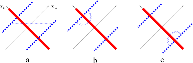
Figure 38: Path integrals describing one-loop diagrams for Wilson-line operators in the shock-wave field background.

Consider at first the diagram shown in Fig. 38a (which corresponds to the case $x_{\ast}>0$, $y_{\ast}<0$). The relevant contribution to the right-hand side of Eq. (7.3) is:

$$- g^{2}\int du[\infty p^{(0)}_{A},up^{(0)}_{A}]_{x}t^{a}[up^{(0)}_{A},-\infty p^{(0)}_{A}]_{x}\otimes\int dv[-\infty p^{(0)}_{A},vp^{(0)}_{A}]_{y}t^{b}$$ (283)

$$\times [vp^{(0)}_{A},\infty p^{(0)}_{A}]_{y}{\hbox{\bf\Big{(}$\!\!$\Big{(}}}up^{(0)}_{A}+x_{\perp}\Big{|}up_{\ast}\{(p^{(0)}_{A\xi}-{\cal P}_{\circ}\frac{p_{2\xi}}{p\cdot p_{2}})$$

$$\times [\frac{1}{{\cal P}^{2}g_{\xi\eta}+2iG_{\xi\eta}}-\frac{1}{{\cal P}^{2}g_{\xi\lambda}+2iG_{\xi\lambda}}(D^{\alpha}G_{\alpha\lambda}\frac{p_{2\rho}}{p\cdot p_{2}}+\frac{p_{2\lambda}}{p\cdot p_{2}}D^{\alpha}G_{\alpha\rho}$$

$$- \frac{p_{2\lambda}}{p\cdot p_{2}}{\cal P}^{\beta}D^{\alpha}G_{\alpha\beta}\frac{p_{2\rho}}{p\cdot p_{2}})\frac{1}{{\cal P}^{2}g_{\rho\eta}+2iF_{\rho\eta}}+\ldots]$$

$$\times (p^{(0)}_{A\eta}-\frac{p_{2\eta}}{p\cdot p_{2}}{\cal P}_{\circ})\}-v\left\{\ldots\right\}p_{\ast}\Big{|}vp^{(0)}_{A}+y_{\perp}{\hbox{\bf\Big{)}$\!\!$\Big{)}}}_{ab}.$$

As we discussed in Sec. 4, terms in parentheses proportional to ${\cal P}_{\circ}$ vanish after integration by parts (see. Eq. (122)). Further, it is easy to check that since the only nonzero component of field strength tensor for the shock wave is $G_{\circ\perp}$ the expression in braces in Eq. (283) can be reduced to ${\cal O}_{\circ\circ}$ where the operator ${\cal O}_{\mu\nu}$ is given by Eq. (7.4). Starting from this point, it is convenient to perform the calculation in the background of the rotated field $B^{\Omega}$ (91) which is $0$ everywhere except the shock-wave wall. (We shall make the rotation back to field $B$ in the final answer). The gauge factors $[\infty,u]t^{a}[u,-\infty]$ and $[\infty,v]t^{b}[v,-\infty]$ in Eq. (283) reduce to $t^{a}[\infty,-\infty]\otimes t^{b}[-\infty,\infty]$ (at $x_{\ast}>0,y_{\ast}<0$) and we obtain:

$$-g^{2}t^{a}U^{\Omega}\otimes t^{b}U^{\dagger\Omega}\int\!du\int\!dv(u-v){\hbox{\bf\Big{(}$\!\!$\Big{(}}}up^{(0)}_{A}+x_{\perp}\Big{|}p_{\ast}{\cal O}^{\Omega}_{\circ\circ}\Big{|}vp^{(0)}_{A}+y_{\perp}{\hbox{\bf\Big{)}$\!\!$\Big{)}}}_{ab}$$ (284)

where we have used the fact that the operator $p_{\ast}$ commutes with ${\cal O}^{\Omega}$. Let us now derive the formula for the $(_{\circ\circ})$ component of the gluon propagator $\hbox{\bf\Big{(}$\!\!$\Big{(}}x\Big{|}{\cal O}^{\Omega}\Big{|}y\hbox{\bf\Big{)}$\!\!$\Big{)}}$ in the shock-wave background. The path-integral representation of $\hbox{\bf\Big{(}$\!\!$\Big{(}}x\Big{|}{\cal O}^{\Omega}_{\circ\circ}\Big{|}y\hbox{\bf\Big{)}$\!\!$\Big{)}}$ has the form

$$\!\!\!\!\!{\hbox{\bf\Big{(}$\!\!$\Big{(}}}x\Big{|}4\frac{1}{{\cal P}^{2}}G^{\xi\Omega}_{~{}~{}\circ}\frac{1}{{\cal P}^{2}}G^{\Omega}_{\xi\circ}\frac{1}{{\cal P}^{2}}-\frac{1}{{\cal P}^{2}}(D^{\alpha}G^{\Omega}_{\alpha\circ}\frac{s_{0}}{2p_{\ast}}$$

$$+ \!\!\!\!\!\frac{s_{0}}{2p_{\ast}}D^{\alpha}G^{\Omega}_{\alpha\nu}-\frac{s_{0}}{2p_{\ast}}{\cal P}^{\beta}D^{\alpha}G^{\Omega}_{\alpha\beta}\frac{s_{0}}{2p_{\ast}})\frac{1}{{\cal P}^{2}}\Big{|}y{\hbox{\bf\Big{)}$\!\!$\Big{)}}}$$

$$= \!\!\!i\int_{0}^{\infty}\!d\tau\int_{0}^{\tau}\!d\tau^{\prime}{\hbox{\bf\Big{(}$\!\!$\Big{(}}}x\Big{|}e^{i(\tau-\tau^{\prime}){\cal P}^{2}}\Big{\{}G^{\alpha\Omega}_{\circ}\int_{0}^{\tau^{\prime}}\!d\tau^{\prime\prime}e^{i(\tau^{\prime}-\tau^{\prime\prime}){\cal P}^{2}}$$

$$\times \!\!\!\!\!G^{\Omega}_{\alpha\circ}e^{i\tau^{\prime\prime}{\cal P}^{2}}-{is_{0}\over 2p_{\ast}}D^{\alpha}G^{\Omega}_{\alpha\circ}e^{i\tau^{\prime\prime}{\cal P}^{2}}\Big{\}}\Big{|}y{\hbox{\bf\Big{)}$\!\!$\Big{)}}}$$

$$= \!\!\!\!\!i\int_{0}^{\infty}\!d\tau{\cal N}^{-1}\int_{x(0)=y}^{x(\tau)=x}\!{\cal D}x(t)e^{-i\int_{0}^{\tau}\!dt{\dot{x}^{2}\over 4}}\{4\int_{0}^{\tau}\!d\tau^{\prime}\int_{0}^{\tau^{\prime}}\!d\tau^{\prime\prime}$$

$$\times \!\!\!\!\!Pe^{ig\int_{\tau^{\prime}}^{\tau}\!dtB^{\Omega}_{\mu}(x(t))\dot{x}_{\mu}(t)}gG^{\Omega}_{\circ i}(x(\tau^{\prime}))Pe^{ig\int^{\tau^{\prime}}_{\tau^{\prime\prime}}\!dtB^{\Omega}_{\mu}(x(t))\dot{x}_{\mu}(t)}\int_{0}^{\tau^{\prime}}\!d\tau^{\prime\prime}$$

$$\times \!\!\!\!\!Pe^{ig\int_{\tau^{\prime\prime}}^{\tau^{\prime}}\!dtB^{\Omega}_{\mu}(x(t))\dot{x}_{\mu}(t)}gG^{\Omega}_{\circ i}(x(\tau^{\prime\prime}))Pe^{ig\int^{\tau^{\prime\prime}}_{0}\!dtB^{\Omega}_{\mu}(x(t))\dot{x}_{\mu}(t)}$$

$$+ \!\!\!\!\!i\int_{0}^{\tau}\!d\tau^{\prime}Pe^{ig\int_{\tau^{\prime}}^{\tau}\!dtB^{\Omega}_{\mu}(x(t))\dot{x}_{\mu}(t)}{s_{0}\over\dot{x_{\ast}}(\tau^{\prime})}gD^{\alpha}G^{\Omega}_{\alpha\circ}(x(\tau^{\prime}))Pe^{ig\int^{\tau^{\prime}}_{0}\!dtB^{\Omega}_{\mu}(x(t))\dot{x}_{\mu}(t)}\}.$$

As we discussed above, the transition through the shock wave occurs in a short time $\sim{1\over\lambda}$ so the gluon has no time to deviate in the transverse directions and therefore the gauge factors in Eq. (7.3) can be approximated by segments of Wilson lines. One obtains then (cf. Eq. (271)):

$${\hbox{\bf\Big{(}$\!\!$\Big{(}}}x\Big{|}{\cal O}^{\Omega}_{\circ\circ}\Big{|}y{\hbox{\bf\Big{)}$\!\!$\Big{)}}}$$

$$= {i\over 2}s_{0}^{2}\int_{0}^{\infty}\!d\tau\int_{0}^{\tau}\!d\tau^{\prime}\int\!dz\delta(z_{*}){\cal N}^{-1}\int_{x(\tau^{\prime})=z}^{x(\tau)=x}\!{\cal D}x(t)\!e^{-i\int_{\tau^{\prime}}^{\tau}\!dt{\dot{x}^{2}\over 4}}$$

$$\times {1\over\dot{x}_{\ast}(\tau^{\prime})}\{2[GG]^{\Omega}(z_{\perp})-i[DG]^{\Omega}(z_{\perp})\}{\cal N}^{-1}\int_{x(0)=y}^{x(\tau^{\prime})=z}\!{\cal D}x(t)e^{-i\int_{\tau^{\prime}}^{\tau}\!dt{\dot{x}^{2}\over 4}},$$

where $[GG]^{\Omega}$ and $[DG]^{\Omega}$ are the notations for the gauge factors (127) calculated for the background field $B^{\Omega}_{\mu}$,

$$\![DG]^{\Omega}(x_{\perp}) = \int du[\infty p_{1},up_{1}]_{x}D^{\alpha}G^{\Omega}_{\alpha\circ}(up_{1}+x_{\perp})[up_{1},-\infty p_{1}]_{x},$$

$$\![GG]^{\Omega}(x_{\perp}) = \int\!du\int\!dv\Theta(u-v)[\infty p_{1},up_{1}]_{x}G^{\xi\Omega}_{\circ}(up_{1}+x_{\perp})$$ (287)

$$\times [up_{1},vp_{1}]_{x}G^{\Omega}_{\xi\circ}(vp_{1}+x_{\perp})[vp_{1},-\infty p_{1}]_{x}.$$

As we noted in Sec. 4, the gauge factor $-i[DG]+2[GG]$ in braces in Eq. (7.3) is in fact the total derivative of $U$ with respect to translations in the perpendicular directions so we get

$${\hbox{\bf\Big{(}$\!\!$\Big{(}}}x\Big{|}{\cal O}^{\Omega}_{\circ\circ}\Big{|}y{\hbox{\bf\Big{)}$\!\!$\Big{)}}} = {i\over 2}s_{0}^{2}\int_{0}^{\infty}\!d\tau\int_{0}^{\tau}\!d\tau^{\prime}\int\!dz\delta(z_{*})$$

$$\times {\cal N}^{-1}\int_{x(\tau^{\prime})=z}^{x(\tau)=x}\!{\cal D}x(t)\!e^{-i\int_{\tau^{\prime}}^{\tau}\!dt{\dot{x}^{2}\over 4}}{1\over\dot{x}_{\ast}(\tau^{\prime})}\vec{\partial}_{\perp}^{2}U^{\Omega}(x_{\perp})$$

$$\times {\cal N}^{-1}\int_{x(0)=y}^{x(\tau^{\prime})=z}\!{\cal D}x(t)e^{-i\int_{\tau^{\prime}}^{\tau}\!dt{\dot{x}^{2}\over 4}}.$$

Using now the path-integral representation for bare propagator (95) and the following formula

$$\int_{0}^{\infty}\!d\tau{\cal N}^{-1}\int^{x(\tau)=x}_{x(0)=y}\!{\cal D}x(t){1\over\dot{x}_{\ast}(0)}e^{-i\int^{\tau}_{0}\!dt{\dot{x}^{2}\over 4}}=i\frac{\ln(x-y)^{2}}{16\pi^{2}(x-y)_{\ast}}$$ (289)

we finally obtain the $(_{\circ\circ})$ component of the gluon propagator in the shock-wave background in the form:

$${\hbox{\bf\Big{(}$\!\!$\Big{(}}}x\Big{|}{\cal O}^{\Omega}_{\circ\circ}\Big{|}y{\hbox{\bf\Big{)}$\!\!$\Big{)}}}={s_{0}^{2}\over 2}\int\!dz\delta(z_{\ast})\frac{\ln(x-z)^{2}}{16\pi^{2}x_{\ast}}$$

$$\times [\vec{\partial}_{\perp}^{2}U^{\Omega}(z_{\perp})\Theta(x_{\ast})\Theta(-y_{\ast})-\vec{\partial}_{\perp}^{2}U^{\dagger\Omega}(z_{\perp})\Theta(-x_{\ast})\Theta(y_{\ast})]\frac{1}{4\pi^{2}(z-y)^{2}},$$

where we have added the similar term corresponding to the case $x_{\ast}<0$, $y_{\ast}>0$. We need also the ${\partial\over\partial x_{\circ}}$ derivative of this propagator (see Eq. (284)) which is

$${\hbox{\bf\Big{(}$\!\!$\Big{(}}}x\Big{|}p_{\ast}{\cal O}^{\Omega}_{\circ\circ}\Big{|}y{\hbox{\bf\Big{)}$\!\!$\Big{)}}}={is_{0}^{2}\over 64\pi^{4}}\int\!dz\frac{\delta(z_{\ast})}{(x-y)^{2}}$$

$$\times [\vec{\partial}_{\perp}^{2}U^{\Omega}(z_{\perp})\Theta(x_{\ast})\Theta(-y_{\ast})-\vec{\partial}_{\perp}^{2}U^{\dagger\Omega}(z_{\perp})\Theta(-x_{\ast})\Theta(y_{\ast})]\frac{1}{(z-y)^{2}}.$$

Substituting now the Eq. (7.3) into Eq. (284) one obtains

$${g^{2}\over 4\pi}{\hbox{\bf\Big{(}$\!\!$\Big{(}}}x_{\perp}\Big{|}\frac{1}{\vec{p}_{\perp}^{2}}\vec{\partial}_{\perp}^{2}U^{\Omega}\frac{1}{\vec{p}_{\perp}^{2}}\Big{|}y_{\perp}{\hbox{\bf\Big{)}$\!\!$\Big{)}}}_{ab}t^{a}U^{\Omega}(x_{\perp})\otimes t^{b}U^{\dagger\Omega}(y_{\perp})$$ (292)

$$+ {g^{2}\over 4\pi}{\hbox{\bf\Big{(}$\!\!$\Big{(}}}x_{\perp}\Big{|}\frac{1}{\vec{p}_{\perp}^{2}}\vec{\partial}_{\perp}^{2}U^{\dagger\Omega}\frac{1}{\vec{p}_{\perp}^{2}}\Big{|}y_{\perp}{\hbox{\bf\Big{)}$\!\!$\Big{)}}}_{ab}U^{\Omega}(x_{\perp})t^{a}\otimes U^{\dagger\Omega}(y_{\perp})t^{b}.$$

which agrees with Eq. (131).

Let us consider now the diagram shown in Fig. 38c. The calculation is very similar to the case of Fig. 38a diagram considered above so we shall only briefly outline the calculation. One starts with the corresponding contribution to the right-hand side of Eq. (7.3) which has the form (cf. (283):

$$- \!\!g^{2}\zeta\int\!du\int\!dv\Theta(u-v)[\infty p^{(0)}_{A}+x_{\perp},up^{(0)}_{A}+x_{\perp}]t^{a}[up^{(0)}_{A}+x_{\perp},vp^{(0)}_{A}+x_{\perp}]$$ (293)

$$\times \!\!t^{b}[vp^{(0)}_{A}+x_{\perp},-\infty p^{(0)}_{A}+x_{\perp}]\otimes U^{\dagger}(y_{\perp})$$

$$\times \!\!{\hbox{\bf\Big{(}$\!\!$\Big{(}}}up^{(0)}_{A}+x_{\perp}\Big{|}up_{\ast}\{(p^{(0)}_{A\xi}-{\cal P}_{\circ}\frac{p_{2\xi}}{p\cdot p_{2}})[\frac{1}{{\cal P}^{2}g_{\xi\eta}+2iG_{\xi\eta}}-\frac{1}{{\cal P}^{2}g_{\xi\lambda}+2iG^{\Omega}_{\xi\lambda}}$$

$$\times \!\!\Big{[}D^{\alpha}G^{\Omega}_{\alpha\lambda}\frac{p_{2\rho}}{p\cdot p_{2}}+\frac{p_{2\lambda}}{p\cdot p_{2}}D^{\alpha}G^{\Omega}_{\alpha\rho}-\frac{p_{2\lambda}}{p\cdot p_{2}}{\cal P}^{\beta}D^{\alpha}G_{\alpha\beta}\frac{p_{2\rho}}{p\cdot p_{2}}\Big{]}$$

$$\times \!\!\frac{1}{{\cal P}^{2}g_{\rho\eta}+2iG_{\rho\eta}}+\ldots](p^{(0)}_{A\eta}-\frac{p_{2\eta}}{p\cdot p_{2}}{\cal P}_{\circ})\}-v\left\{\ldots\right\}p_{\ast}\Big{|}vp^{(0)}_{A}+x_{\perp}{\hbox{\bf\Big{)}$\!\!$\Big{)}}}_{ab}.$$

As we demonstrated in Sec. 4, the terms in parentheses proportional to ${\cal P}_{\circ}$ vanish and after that the operator in braces reduce to ${\cal O}_{\circ\circ}$. Again, it is convenient to make a gauge transformation to the rotated field (91) which is 0 everywhere except the shock wave. Then the gauge factor $[\infty,u]t^{a}[u,v]t^{b}[v,-\infty]$ in Eq. (293) simplifies to $t^{a}[\infty,-\infty]t^{b}$ (at $x_{\ast}>0,y_{\ast}<0$) and we obtain

$$-g^{2}t^{a}U^{\Omega}t^{b}\otimes U^{\dagger\Omega}\int\!du\int\!dv(u-v){\hbox{\bf\Big{(}$\!\!$\Big{(}}}up^{(0)}_{A}+x_{\perp}\Big{|}p_{\ast}{\cal O}^{\Omega}_{\circ\circ}\Big{|}vp^{(0)}_{A}+x_{\perp}{\hbox{\bf\Big{)}$\!\!$\Big{)}}}_{ab}.$$ (294)

Using the expression (7.3) for the gluon propagator in the shock-wave background we can reduce Eq. (294) to

$$-{g^{2}\over 4\pi}t^{a}U^{\Omega}(x_{\perp})t^{b}\otimes U^{\dagger\Omega}(y_{\perp}){\hbox{\bf\Big{(}$\!\!$\Big{(}}}x_{\perp}\Big{|}\frac{1}{\vec{p}_{\perp}^{2}}(\vec{\partial}_{\perp}^{2}U^{\Omega})\frac{1}{\vec{p}_{\perp}^{2}}\Big{|}x_{\perp}{\hbox{\bf\Big{)}$\!\!$\Big{)}}}_{ab}.$$ (295)

The contribution of the diagram in Fig. 38b differs from Eq. (295) only in change $U\leftrightarrow U^{\dagger},~{}x\leftrightarrow y$. Combining these expressions, one obtains the answer in the rotated field (91) in the form

$$\!\!\!\!\!{g^{2}\over 16\pi^{3}}\int\!dz_{\perp}\Bigg{\{}\Big{[}\{U^{\dagger\Omega}(z_{\perp})U^{\Omega}(x_{\perp})\}^{k}_{j}\{U^{\Omega}(z_{\perp})U^{\dagger\Omega}(y_{\perp})\}^{i}_{l}$$

$$+ \!\!\!\!\!\{U^{\Omega}(x_{\perp})U^{\dagger\Omega}(z_{\perp})\}^{i}_{l}\{U^{\dagger\omega}(y_{\perp})U^{\Omega}(z_{\perp})\}^{k}_{j}$$

$$- \!\!\!\!\!\delta^{k}_{j}\{U^{\Omega}(x_{\perp})U^{\dagger\Omega}(y_{\perp})\}^{i}_{l}-\delta^{i}_{l}\{U^{\dagger\Omega}(y_{\perp})U^{\Omega}(x_{\perp})\}^{k}_{j}\Big{]}\frac{(\vec{x}-\vec{z},\vec{y}-\vec{z})_{\perp}}{(\vec{x}-\vec{z})_{\perp}^{2}(\vec{y}-\vec{z})_{\perp}^{2}}$$

$$- \!\!\!\!\!\Big{[}\{U^{\Omega}(z_{\perp})\}^{i}_{j}{\rm Tr}\{U^{\Omega}(x_{\perp})U^{\dagger\Omega}(z_{\perp})\}-N_{c}\{U^{\Omega}(x_{\perp})\}^{i}_{j})U^{\dagger\Omega}(y_{\perp})^{k}_{l}\frac{1}{(\vec{x}-\vec{z})_{\perp}^{2}}$$

$$- \!\!\!\!\!\{U^{\Omega}(x_{\perp})\}^{i}_{j}[U^{\dagger\Omega}(z_{\perp})^{k}_{l}{\rm Tr}\{U^{\Omega}(z_{\perp})U^{\dagger\Omega}(y_{\perp})\}-N_{c}\{U^{\dagger\Omega}(y_{\perp})\}^{k}_{l})\Big{]}\frac{1}{(\vec{y}-\vec{z})_{\perp}^{2}}\Bigg{\}}.$$

Now we must perform the gauge rotation back to the “original” field $B_{\mu}$. The answer is especially simple if we consider the evolution of the gauge-invariant operator such as $Tr\{U(x_{\perp})[x_{\perp},y_{\perp}]_{-}U^{\dagger}(y_{\perp})[y_{\perp},x_{\perp}]_{+}\}$ where the Wilson lines are connected by gauge segments at the infinity. We have then

$$\zeta{\partial\over\partial\zeta}\langle{\rm Tr}\{{\hat{U}^{\zeta}}(x_{\perp})[x_{\perp},y_{\perp}]_{-}{\hat{U}^{\dagger\zeta}}(y_{\perp})[y_{\perp},x_{\perp}]_{+}\}\rangle_{A}=$$ (297)

$$= -{\alpha_{s}\over 4\pi^{2}}\int\!dz_{\perp}{(\vec{x}-\vec{y})_{\perp}^{2}\over(\vec{x}-\vec{z})_{\perp}^{2}(\vec{z}-\vec{y})_{\perp}^{2}}$$

$$\times \Bigg{(}{\rm Tr}\{U(x_{\perp})[x_{\perp},z_{\perp}]_{-}U^{\dagger}(z_{\perp})[z_{\perp},x_{\perp}]_{+}\}$$

$$\times {\rm Tr}\{U(z_{\perp})[z_{\perp},y_{\perp}]_{-}U^{\dagger}(y_{\perp})[y_{\perp},z_{\perp}]_{+}\}$$

$$- N_{c}{\rm Tr}\{U(x_{\perp})[x_{\perp},y_{\perp}]_{-}U^{\dagger}(y_{\perp})[y_{\perp},x_{\perp}]_{+}\}\Bigg{)},$$

where we have replaced the end gauge factors like $\Omega(\infty p_{1}+x_{\perp})\Omega^{\dagger}(\infty p_{1}+y_{\perp})$ and $\Omega(-\infty p_{1}+x_{\perp})\Omega^{\dagger}(-\infty p_{1}+y_{\perp})$ by segments of gauge line $[x_{\perp},y_{\perp}]_{+}$ and $[x_{\perp},y_{\perp}]_{-}$, respectively. Since the background field $B_{\mu}$ is a pure gauge outside the shock wave the specific form of the contour in Eq. (297) does not matter as long as it has the same initial and final points. Finally, note that the gauge factors in the right-hand side of Eq. (297) preserve their form after rescaling back to the field $A_{\mu}$ so we reproduce the Eq. (136).

In the general case, the evolution of the 2$n$-line operators such as
${\rm Tr}\{UU^{\dagger}\}{\rm Tr}\{UU^{\dagger}\}...{\rm Tr}\{UU^{\dagger}\}$ come from either self-interaction diagrams or from the pair-interactions ones (see Fig. 39).

Figure 39: Typical diagrams for the one-loop evolution of the $n$-line operator.

These pair-wise kernels have the form ($U_{x}\equiv U(x_{\perp})$, etc.)

$$\zeta\frac{\partial}{\partial\zeta}\{U_{x}\}^{i}_{j}\{U^{\dagger}_{y}\}^{k}_{l}~{}=~{}{g^{2}\over 16\pi^{3}}\int dz_{\perp}\frac{(\vec{x}-\vec{z},\vec{y}-\vec{z})_{\perp}}{(\vec{x}-\vec{z})_{\perp}^{2}(\vec{y}-\vec{z})_{\perp}^{2}}$$

$$\times \Bigg{(}\{U^{\dagger}_{z}U_{x}\}^{k}_{j}\{U_{z}U^{\dagger}_{y}\}^{i}_{l}+\{U_{x}U^{\dagger}_{z}\}^{i}_{l}\{U^{\dagger}_{y}U_{z}\}^{k}_{j}-\delta^{k}_{j}\{U_{x}U^{\dagger}_{y}\}^{i}_{l}-\delta^{i}_{l}\{U^{\dagger}_{y}U_{x}\}^{k}_{j}\Bigg{)},$$

$$\zeta\frac{\partial}{\partial\zeta}\{U_{x}\}^{i}_{j}\{U_{y}\}^{k}_{l}~{}=~{}-{g^{2}\over 16\pi^{3}}\int dz_{\perp}\frac{(\vec{x}-\vec{z},\vec{y}-\vec{z})_{\perp}}{(\vec{x}-\vec{z})_{\perp}^{2}(\vec{y}-\vec{z})_{\perp}^{2}}$$

$$\times \Bigg{(}\{U_{z}\}^{i}_{l}\{U_{y}U^{\dagger}_{z}U_{x}\}^{k}_{j}+\{U_{x}U^{\dagger}_{z}U_{y}\}^{i}_{l}\{U_{z}\}^{k}_{j}-\{U_{x}\}^{i}_{l}\{U_{y}\}^{k}_{j}-\{U_{y}\}^{i}_{l}\{U_{x}\}^{k}_{j}\Bigg{)},$$

$$\zeta\frac{\partial}{\partial\zeta}\{U^{\dagger}_{x}\}^{i}_{j}\{U^{\dagger}_{y}\}^{k}_{l}~{}=~{}-{g^{2}\over 16\pi^{3}}\int dz_{\perp}\frac{(\vec{x}-\vec{z},\vec{y}-\vec{z})_{\perp}}{(\vec{x}-\vec{z})_{\perp}^{2}(\vec{y}-\vec{z})_{\perp}^{2}}$$

$$\times \Bigg{(}\{U^{\dagger}_{z}\}^{i}_{l}\{U^{\dagger}_{y}U_{z}U^{\dagger}_{x}\}^{k}_{j}+\{U^{\dagger}_{x}U_{z}U^{\dagger}_{y}\}^{i}_{l}\{U^{\dagger}_{z}\}^{k}_{j}-\{U^{\dagger}_{x}\}^{i}_{l}\{U^{\dagger}_{y}\}^{k}_{j}-\{U^{\dagger}_{y}\}^{i}_{l}\{U^{\dagger}_{x}\}^{k}_{j}\Bigg{)}$$

for the pair-interaction diagrams in Fig. 39a and

$$\zeta\frac{\partial}{\partial\zeta}\{U_{x}\}^{i}_{j} = -{g^{2}\over 16\pi^{3}}\int dz_{\perp}[U_{z}{\rm Tr}\{U_{x}U^{\dagger}_{z}\}-N_{c}U_{x}]\frac{1}{(\vec{x}-\vec{z})_{\perp}^{2}},$$

$$\zeta\frac{\partial}{\partial\zeta}\{U^{\dagger}_{x}\}^{i}_{j} = -{g^{2}\over 16\pi^{3}}\int dz_{\perp}[U^{\dagger}_{z}{\rm Tr}\{U_{z}U^{\dagger}_{x}\}-N_{c}U^{\dagger}_{x}]\frac{1}{(\vec{x}-\vec{z})_{\perp}^{2}},$$ (299)

for the self-interaction diagrams of Fig. 39b type.

7.4 Gluon propagator in the axial gauge.

Our aim here is to derive the expression for the gluon propagator in the external field in the axial gauge. The propagator of the “quantum” gauge field $A^{q}$ in the external “classical” field $A^{cl}$ in the axial gauge $e_{\mu}A_{\mu}=0$ can be represented as the following functional integral:

$$G_{\mu\nu}^{ab}(x,y) = \lim_{w\rightarrow 0}N^{-1}\int DAA^{qa}_{\mu}(x)A^{qb}_{\nu}(y)$$

$$\times e^{i\int dz{\rm Tr}\{A^{q}_{\alpha}(z)(D^{2}g^{\alpha\beta}-D^{\alpha}D^{\beta}-2iF_{cl}^{\alpha\beta}-{1\over w}e^{\alpha}e^{\beta})A^{q}_{\beta}(z)\}},$$

where $D_{\mu}=\partial_{\mu}-igA^{cl}_{\mu}$. Hereafter we shall omit the label “cl” from the external field. This propagator can be formally written down as

$$iG^{ab}_{\mu\nu}(x,y)={\hbox{\bf\Big{(}$\!\!$\Big{(}}}x\Big{|}\frac{1}{\Box^{\mu\nu}-{\cal P}^{\mu}{\cal P}^{\nu}+\frac{1}{w}e^{\mu}e^{\nu}}\Big{|}y{\hbox{\bf\Big{)}$\!\!$\Big{)}}}^{ab},$$ (301)

where $\Box^{\mu\nu}={\cal P}^{2}g^{\mu\nu}+2iF^{\mu\nu}$. It is easy to check that the operator in right-hand side of Eq. (301) satisfies the recursion formula

$$\frac{1}{\Box^{\mu\nu}-{\cal P}^{\mu}{\cal P}^{\nu}+{e^{\mu}e^{\nu}\over w}} = (\delta_{\mu}^{\xi}-{\cal P}_{\mu}\frac{e^{\xi}}{{\cal P}e})\frac{1}{\Box^{\xi\eta}}(\delta_{\nu}^{\eta}-\frac{e^{\eta}}{{\cal P}e}{\cal P}_{\nu})+{\cal P}_{\mu}\frac{w}{({\cal P}e)^{2}}{\cal P}_{\nu}$$ (302)

$$- \frac{1}{\Box^{\mu\alpha}-{\cal P}^{\mu}{\cal P}^{\alpha}+{e^{\mu}e^{\alpha}\over w}}(D_{\lambda}F^{\lambda\alpha}\frac{e^{\xi}}{{\cal P}e}-{\cal P}^{\alpha}\frac{1}{{\cal P}^{2}}D_{\lambda}F^{\lambda\xi})$$

$$\times \frac{1}{\Box^{\xi\eta}}(\delta_{\nu}^{\eta}-\frac{e^{\eta}}{{\cal P}e}{\cal P}_{\nu})$$

which gives the propagator as an expansion in powers of the operator $D_{\lambda}F^{a}_{\lambda\alpha}=-g\bar{\psi}t^{a}\gamma_{\alpha}\psi$. We shall see below that in the leading logarithmic approximation we need the terms not higher than the first nontrivial order in this operator. With this accuracy

$$\frac{1}{\Box^{\mu\nu}-{\cal P}^{\mu}{\cal P}^{\nu}+\frac{1}{w}e^{\mu}e^{\nu}} = (\delta_{\mu}^{\xi}-{\cal P}_{\mu}\frac{e^{\xi}}{{\cal P}e})\frac{1}{\Box^{\xi\eta}}(\delta_{\nu}^{\eta}-\frac{e^{\eta}}{{\cal P}e}{\cal P}_{\nu})+{\cal P}_{\mu}\frac{w}{({\cal P}e)^{2}}{\cal P}_{\nu}$$ (303)

$$- (\delta_{\mu}^{\xi}-{\cal P}_{\mu}\frac{e^{\xi}}{{\cal P}e})\frac{1}{\Box^{\xi\eta}}\Big{(}D_{\lambda}F^{\lambda\eta}\frac{e^{\rho}}{{\cal P}e}+\frac{e^{\eta}}{{\cal P}e}D_{\lambda}F^{\lambda\rho}$$

$$- \frac{e^{\eta}}{{\cal P}e}{\cal P}^{\beta}D_{\alpha}F^{\alpha\beta}\frac{e^{\rho}}{{\cal P}e}\Big{)}\frac{1}{\Box^{\rho\sigma}}(\delta_{\nu}^{\sigma}-\frac{e^{\sigma}}{{\cal P}e}{\cal P}_{\nu}).$$

We take now $w\rightarrow 0$, obtaining the propagator in external field in axial gauge in the form

$$iG_{\mu\nu}^{ab}(x,y) = (\delta_{\mu}^{\xi}-{\cal P}_{\mu}\frac{e^{\xi}}{{\cal P}e})\frac{1}{\Box^{\xi\eta}}(\delta_{\nu}^{\eta}-\frac{e^{\eta}}{{\cal P}e}{\cal P}_{\nu})-(\delta_{\mu}^{\xi}-{\cal P}_{\mu}\frac{e^{\xi}}{{\cal P}e})\frac{1}{\Box^{\xi\eta}}$$ (304)

$$\times \Big{(}D_{\lambda}F^{\lambda\eta}\frac{e^{\rho}}{{\cal P}e}+\frac{e^{\eta}}{{\cal P}e}D_{\lambda}F^{\lambda\rho}-\frac{e^{\eta}}{{\cal P}e}{\cal P}^{\beta}D_{\alpha}F^{\alpha\beta}\frac{e^{\rho}}{{\cal P}e}\Big{)}$$

$$\times \frac{1}{\Box^{\rho\sigma}}(\delta_{\nu}^{\sigma}-\frac{e^{\sigma}}{{\cal P}e}{\cal P}_{\nu})+\ldots$$

where the dots stand for the terms of second (and higher) order in $D^{\lambda}F_{\lambda\rho}$. It can be demonstrated that for our purposes a first few terms of the expansion of operators ${1\over\Box}$ in powers of $F_{\xi\eta}$ are enough, namely

$$iG_{\mu\nu}^{ab}(x,y)=(\delta_{\mu}^{\xi}-{\cal P}_{\mu}\frac{e^{\xi}}{{\cal P}e})\left[\frac{\delta_{\xi\eta}}{{\cal P}^{2}}-2i\frac{1}{{\cal P}^{2}}F_{\xi\eta}\frac{1}{{\cal P}^{2}}+{\cal O}_{\xi\eta}\right](\delta_{\nu}^{\eta}-\frac{e^{\eta}}{{\cal P}e}{\cal P}_{\nu})+\ldots$$ (305)

where the operator ${\cal O}$ stands for

$${\cal O}_{\mu\nu} = 4\frac{1}{{\cal P}^{2}}F^{\xi}_{~{}~{}\mu}\frac{1}{{\cal P}^{2}}F_{\xi\nu}\frac{1}{{\cal P}^{2}}$$

$$- \frac{1}{{\cal P}^{2}}(D^{\alpha}F_{\alpha\mu}\frac{p_{2\nu}}{p\cdot p_{2}}+\frac{p_{2\mu}}{p\cdot p_{2}}D^{\alpha}F_{\alpha\nu}-\frac{p_{2\mu}}{2p\cdot p_{2}}{\cal P}^{\beta}D^{\alpha}F_{\alpha\beta}\frac{p_{2\nu}}{2p\cdot p_{2}})\frac{1}{{\cal P}^{2}}.$$

7.5 First-order effective action.

As we discussed in Sec. 5, in order to calculate the effective action semiclassically we can start with the trial configuration (208). Making the shift $A\rightarrow A+{\bar{A}}^{(0)}$ in the functional integral (200), we obtain

$$e^{iS_{\rm eff}} = \int\!D\!A\ \exp i\Bigg{\{}\int dx_{\perp}V^{a}_{i}(x_{\perp})U^{ai}(x_{\perp})+2\int dx_{\perp}\Delta^{a}_{i}(x_{\perp})A^{ai}(0,x_{\perp})$$ (307)

$$+ 2{\rm Tr}\int dx_{\perp}\Big{[}-{1\over 2}[U^{i},\Delta_{i}]W_{1}+\big{(}L_{1}+{1\over 2}[U^{i},\Delta_{i}]\big{)}W_{2}$$

$$- {1\over 2}[V^{i},\Delta_{i}]Y_{1}+\big{(}-L_{1}+{1\over 2}[V^{i},\Delta_{i}]\big{)}Y_{2}\Big{]}$$

$$+ {1\over 2}\int d^{4}xA^{a\mu}\left({\bar{D}}^{2}g_{\mu\nu}-2ig{\bar{F}}_{\mu\nu}+g^{2}{\cal G}_{\mu\nu}\right)^{ab}A^{b\mu}+O(A^{3})\Bigg{\}}$$

where

$$Y_{1}(x_{\perp})=[x_{\perp}+\infty p_{1},x_{\perp}]^{(1)}, Y_{2}(x_{\perp})=[x_{\perp},x_{\perp}-\infty p_{1}]^{(1)},$$

$$W_{1}(x_{\perp})=[x_{\perp}+\infty p_{2},x_{\perp}]^{(1)}, W_{2}(x_{\perp})=[x_{\perp},x_{\perp}-\infty p_{2}]^{(1)},$$ (308)

and the operator ${\cal G}_{\mu\nu}$ is the second variational derivative of the source term with respect to $A_{\mu}$, $A_{\nu}$. The non-zero components of ${\cal G}_{\mu\nu}$ are

$${\cal G}_{\bullet\bullet}=\delta({2\over s}x_{\ast})\big{(}\partial_{i}-i[V_{i},)U^{i}{s/2\over i\partial_{\ast}},\qquad{\cal G}_{\ast\ast}=\delta({2\over s}x_{\bullet})\big{(}\partial_{i}-i[U_{i},)V^{i}{s/2\over i\partial_{\bullet}},$$ (309)

while all other components vanish. In the first order in our cluster expansion we obtain

$$S^{(1)}_{\rm eff} = -2\hbox{\bf\Big{(}$\!\!$\Big{(}}0,\Delta_{i}^{a}\Big{|}\left({1\over{\bar{D}}^{2}g_{ik}-2ig{\bar{F}}_{ik}}\right)^{ab}|0,\Delta_{k})$$

$$+{2g^{2}\over s^{2}}\Bigg{\{}\hbox{\bf\Big{(}$\!\!$\Big{(}}0,L_{1}\Big{|}{p_{2}^{\mu}\over\alpha+i\epsilon}+\hbox{\bf\Big{(}$\!\!$\Big{(}}0,[U_{i},\Delta_{i}]\Big{|}{p_{2}^{\mu}\over\alpha}-\hbox{\bf\Big{(}$\!\!$\Big{(}}0,L_{1}\Big{|}{p_{1}^{\mu}\over\beta+i\epsilon}+\hbox{\bf\Big{(}$\!\!$\Big{(}}0,[V_{i},\Delta_{i}]\Big{|}{p_{1}^{\mu}\over\beta}\Bigg{\}}^{a}$$

$$\times\left({1\over{\bar{D}}^{2}g_{\mu\nu}-2ig{\bar{F}}_{\mu\nu}+g^{2}{\cal G}_{\mu\nu}}\right)^{ab}$$

$$\times\Bigg{\{}{p_{2}^{\nu}\over\alpha-i\epsilon}\Big{|}0,L_{1}\hbox{\bf\Big{)}$\!\!$\Big{)}}+{p_{2}^{\nu}\over\alpha}\Big{|}0,[U^{i},\Delta_{i}]\hbox{\bf\Big{)}$\!\!$\Big{)}}-{p_{1}^{\nu}\over\beta-i\epsilon}\Big{|}0,L_{1}\hbox{\bf\Big{)}$\!\!$\Big{)}}+{p_{1}^{\nu}\over\beta}\Big{|}0,[V^{i},\Delta_{i}]\hbox{\bf\Big{)}$\!\!$\Big{)}}\Bigg{\}}$$

where ${1\over\alpha}\equiv{1\over 2}({1\over\alpha-i\epsilon}+{1\over\alpha+i\epsilon})$ ( similarly for ${1\over\beta}$) and $\Big{|}0,\Delta_{i}\hbox{\bf\Big{)}$\!\!$\Big{)}}\equiv\int dz_{\perp}\Big{|}0,z_{\perp}\hbox{\bf\Big{)}$\!\!$\Big{)}}\Delta_{i}(z_{\perp})$ etc. We will now demonstrate that with $O[U,V]^{2}$ accuracy one can reduce ${1\over{\bar{D}}^{2}g_{\mu\nu}-2ig{\bar{F}}_{\mu\nu}+g^{2}{\cal G}_{\mu\nu}}$ in right-hand side of Eq. (7.5) to ${g_{\mu\nu}\over{\bar{D}}^{2}}$. Indeed,

$${1\over\bar{D}^{2}g_{\mu\nu}-2ig\bar{F}_{\mu\nu}+g^{2}{\cal G}_{\mu\nu}}$$

$$= {g_{\mu\nu}\over\bar{D}^{2}}+2ig{1\over\bar{D}^{2}}\bar{F}_{\mu\nu}{1\over\bar{D}^{2}}-4g^{2}{1\over\bar{D}^{2}}\bar{F}_{\mu\xi}{1\over\bar{D}^{2}}\bar{F}_{\xi\nu}{1\over\bar{D}^{2}}-g^{2}{1\over\bar{D}^{2}}{\cal G}_{\mu\nu}{1\over\bar{D}^{2}}+\ldots.$$

It is easy to note that the term $\sim{1\over\bar{D}^{2}}\bar{F}_{\mu\nu}{1\over\bar{D}^{2}}$ does not contribute to right-hand side of Eq. (7.5) because the relevant components of ${\bar{F}}_{\mu\nu}$ vanish: ${\bar{F}}_{ik}={\bar{F}}_{\ast\bullet}=0$. Let us prove that the last term in the right-hand side of Eq. (7.5) leads to the contributions $\sim[U,V]^{3}$. Consider the first term in the right-hand side of Eq. (309). The corresponding contribution is ${1\over{\bar{D}}^{2}}\bar{F}_{i\bullet}{1\over{\bar{D}}^{2}}\bar{F}_{\ast k}{1\over{\bar{D}}^{2}}+(\bullet\leftrightarrow\ast)$. Because $\bar{F}_{\ast i}=U_{i}+O(\Delta_{i}),~{}~{}\bar{F}_{i\bullet}=V_{i}+O(\Delta_{i})$ this term is actually proportional to $\Delta_{i}{1\over{\bar{D}}^{2}}V_{i}{1\over{\bar{D}}^{2}}U_{k}{1\over{\bar{D}}^{2}}\Delta_{k}\sim[U,V]^{3}$. Let us now turn our attention to the second term in the right-hand side of Eq. (7.5). The relevant contributions have the structure $L_{1}\left({4\over{\bar{D}}^{2}}{\bar{F}}_{\bullet i}{1\over{\bar{D}}^{2}}{\bar{F}}_{\bullet i}{1\over{\bar{D}}^{2}}-{1\over{\bar{D}}^{2}}{\cal G}_{\bullet\bullet}\right)L_{1}{1\over{\bar{D}}^{2}}$, $L_{1}{1\over{\bar{D}}^{2}}{\bar{F}}_{\bullet i}{1\over{\bar{D}}^{2}}{\bar{F}}_{\ast i}{1\over{\bar{D}}^{2}}L_{1}$, $[V_{i},\Delta_{i}]\left({1\over{\bar{D}}^{2}}{\bar{F}}_{\bullet i}{1\over{\bar{D}}^{2}}{\bar{F}}_{\bullet i}{1\over{\bar{D}}^{2}}+{1\over{\bar{D}}^{2}}{\cal G}_{\bullet\bullet}{1\over{\bar{D}}^{2}}\right)[V_{i},\Delta_{i}]$, $[V_{i},\Delta_{i}]{1\over{\bar{D}}^{2}}{\bar{F}}_{\bullet i}{1\over{\bar{D}}^{2}}{\bar{F}}_{\ast i}{1\over{\bar{D}}^{2}}[U_{i},\Delta_{i}]$,
and similar expressions with $U\leftrightarrow V$, $\ast\leftrightarrow\bullet$. All of them are clearly $\sim[U,V]^{3}$ except the first term which is

$$g^{2}\hbox{\bf\Big{(}$\!\!$\Big{(}}0,L_{1}\Big{|}{1\over\beta+i\epsilon}\left({4\over\bar{D}^{2}}{\bar{F}}_{\bullet i}{1\over{\bar{D}}^{2}}{\bar{F}}_{\bullet i}{1\over{\bar{D}}^{2}}-{1\over{\bar{D}}^{2}}{\cal G}_{\bullet\bullet}{1\over{\bar{D}}^{2}}\right){1\over\beta-i\epsilon}\Big{|}0,L_{1}\hbox{\bf\Big{)}$\!\!$\Big{)}}.$$ (312)

If we neglect the $[U,V]^{3}$ terms in cluster expansion, the Green function in braces in right-hand side of Eq. (312) should be taken in the $U_{i}\theta(x_{\ast})$ background. This Green function has the form

$$\hbox{\bf\Big{(}$\!\!$\Big{(}}x\Big{|}-4{1\over{\bar{D}}^{2}}{\bar{F}}_{\bullet i}{1\over{\bar{D}}^{2}}{\bar{F}}_{\bullet i}{1\over{\bar{D}}^{2}}+{1\over{\bar{D}}^{2}}{\cal G}_{\bullet\bullet}{1\over{\bar{D}}^{2}}\Big{|}y\hbox{\bf\Big{)}$\!\!$\Big{)}}~{}=~{}\hbox{\bf\Big{(}$\!\!$\Big{(}}x\Big{|}{\cal O}_{\bullet\bullet}\Big{|}y\hbox{\bf\Big{)}$\!\!$\Big{)}}$$

$$= -i\theta(x_{\ast})\theta(-y_{\ast})U^{\dagger}(x_{\perp})\int dz\delta(z_{\ast})\hbox{\bf\Big{(}$\!\!$\Big{(}}x\Big{|}{1\over p^{2}\alpha}\Big{|}z\hbox{\bf\Big{)}$\!\!$\Big{)}}\vec{\partial}_{\perp}^{2}U(z_{\perp})\hbox{\bf\Big{(}$\!\!$\Big{(}}z\Big{|}{1\over p^{2}}\Big{|}y\hbox{\bf\Big{)}$\!\!$\Big{)}},$$

plus the similar term $\sim\theta(-x_{\ast})\theta(y_{\ast})$. It is easy to see that the terms $\sim\theta(x_{\ast})\theta(-y_{\ast})$ or $\sim\theta(-x_{\ast})\theta(y_{\ast})$ do not contribute to Eq. (312) — recall that this term comes from the contraction of $L_{1}W_{2}(x)$ and $L_{1}Y_{2}(y)$ where both $x_{\ast},y_{\ast}<0$.

Thus, the $[U,V]^{2}$ term in cluster expansion of Eq. (7.5) reduces to

$$S^{(1)}_{\rm eff}~{}=~{}\hbox{\bf\Big{(}$\!\!$\Big{(}}0,\Delta_{i}\Big{|}{-2\over{\bar{D}}^{2}}\Big{|}0,\Delta_{i}\hbox{\bf\Big{)}$\!\!$\Big{)}}$$ (314)

$$-~{}{g^{2}\over s}\hbox{\bf\Big{(}$\!\!$\Big{(}}0,L_{1}\Big{|}\Big{[}{1\over\alpha+i\epsilon}{1\over{\bar{D}}^{2}}{1\over\beta-i\epsilon}+{1\over\beta+i\epsilon}{1\over{\bar{D}}^{2}}{1\over\alpha-i\epsilon}\Big{]}\Big{|}0,L_{1}\hbox{\bf\Big{)}$\!\!$\Big{)}}$$

$$-~{}{g^{2}\over s}\hbox{\bf\Big{(}$\!\!$\Big{(}}0,L_{1}\Big{|}{1\over\beta+i\epsilon}{1\over{\bar{D}}^{2}}{1\over\alpha}\Big{|}0,[U^{i},\Delta_{i}]\hbox{\bf\Big{)}$\!\!$\Big{)}}+{g^{2}\over s}\hbox{\bf\Big{(}$\!\!$\Big{(}}0,L_{1}\Big{|}{1\over\alpha+i\epsilon}{1\over{\bar{D}}^{2}}{1\over\beta}\Big{|}0,[V^{i},\Delta_{i}]\hbox{\bf\Big{)}$\!\!$\Big{)}}$$

$$-~{}{g^{2}\over s}\hbox{\bf\Big{(}$\!\!$\Big{(}}0,[U^{i},\Delta_{i}]\Big{|}{1\over\alpha}{1\over{\bar{D}}^{2}}{1\over\beta-i\epsilon}\Big{|}0,L_{1}\hbox{\bf\Big{)}$\!\!$\Big{)}}+{g^{2}\over s}\hbox{\bf\Big{(}$\!\!$\Big{(}}0,[V_{i},\Delta^{i}]\Big{|}{1\over\beta}{1\over{\bar{D}}^{2}}{1\over\alpha-i\epsilon}\Big{|}0,L_{1}\hbox{\bf\Big{)}$\!\!$\Big{)}}.$$

It is easy to see that the remaining Green function connect points belonging to the different boundaries of the same sector in Fig. 40.

Figure 40: Trial field configuration.

It may be demonstrated that up to $[U,V]$ accuracy the only effect of the background field on the Green function with the arguments belonging to the same sector is the corresponding gauge factor: $\hbox{\bf\Big{(}$\!\!$\Big{(}}x\Big{|}{1\over D^{2}}\Big{|}y\hbox{\bf\Big{)}$\!\!$\Big{)}}=\Omega^{\dagger}(x_{\perp})\hbox{\bf\Big{(}$\!\!$\Big{(}}x\Big{|}{-1\over p^{2}}\Big{|}y\hbox{\bf\Big{)}$\!\!$\Big{)}}\Omega^{\dagger}(y_{\perp})$, where $\Omega$ is $U,~{}V$, or $\Lambda$. We obtain

$$\hbox{\bf\Big{(}$\!\!$\Big{(}}0,x_{\perp}\Big{|}{1\over\alpha+i\epsilon}{1\over D^{2}}{1\over\beta-i\epsilon}\Big{|}0,y_{\perp}\hbox{\bf\Big{)}$\!\!$\Big{)}}=\hbox{\bf\Big{(}$\!\!$\Big{(}}0,x_{\perp}\Big{|}{1\over\alpha+i\epsilon}{-1\over p^{2}+i\epsilon}{1\over\beta-i\epsilon}\Big{|}0,y_{\perp}\hbox{\bf\Big{)}$\!\!$\Big{)}},$$ (315)

$$\hbox{\bf\Big{(}$\!\!$\Big{(}}0,x_{\perp}\Big{|}{1\over\alpha+i\epsilon}{1\over D^{2}}{1\over\beta+i\epsilon}\Big{|}0,y_{\perp}\hbox{\bf\Big{)}$\!\!$\Big{)}}=U^{\dagger}_{x}\hbox{\bf\Big{(}$\!\!$\Big{(}}0,x_{\perp}\Big{|}{1\over\alpha+i\epsilon}{-1\over p^{2}+i\epsilon}{1\over\beta+i\epsilon}\Big{|}0,y_{\perp}\hbox{\bf\Big{)}$\!\!$\Big{)}}U_{y},$$

$$\hbox{\bf\Big{(}$\!\!$\Big{(}}0,x_{\perp}\Big{|}{1\over\alpha-i\epsilon}{1\over D^{2}}{1\over\beta-i\epsilon}\Big{|}0,y_{\perp}\hbox{\bf\Big{)}$\!\!$\Big{)}}=V^{\dagger}_{x}\hbox{\bf\Big{(}$\!\!$\Big{(}}0,x_{\perp}\Big{|}{1\over\alpha-i\epsilon}{-1\over p^{2}+i\epsilon}{1\over\beta-i\epsilon}\Big{|}0,y_{\perp}\hbox{\bf\Big{)}$\!\!$\Big{)}}V_{y}.$$

In the leading log approximation 

$$\hbox{\bf\Big{(}$\!\!$\Big{(}}0,x_{\perp}\Big{|}{-1\over p^{2}+i\epsilon}\Big{|}0,y_{\perp}\hbox{\bf\Big{)}$\!\!$\Big{)}}={i\over 4\pi}\ln{\sigma\over\sigma^{\prime}}\delta^{2}(x_{\perp}-y_{\perp}),$$ (317)

and

$$\hbox{\bf\Big{(}$\!\!$\Big{(}}0,x_{\perp}\Big{|}{1\over\alpha\pm i\epsilon}{-2/s\over p^{2}+i\epsilon}{1\over\beta-i\epsilon}\Big{|}0,y_{\perp}\hbox{\bf\Big{)}$\!\!$\Big{)}}\!\!\!\! = \!\!\!\!\hbox{\bf\Big{(}$\!\!$\Big{(}}0,x_{\perp}\Big{|}{1\over\alpha\pm i\epsilon}{-2/s\over p^{2}+i\epsilon}{1\over\beta+i\epsilon}\Big{|}0,y_{\perp}\hbox{\bf\Big{)}$\!\!$\Big{)}}$$ (318)

$$= \!\!\!\!{i\over 2\pi}\ln{\sigma\over\sigma^{\prime}}\hbox{\bf\Big{(}$\!\!$\Big{(}}x_{\perp}\Big{|}{1\over\vec{p}_{\perp}^{2}}\Big{|}y_{\perp}\hbox{\bf\Big{)}$\!\!$\Big{)}},$$

so we get

$$S^{(1)}_{\rm eff} = {-i\over 2\pi}\ln{\sigma\over\sigma^{\prime}}\Bigg{(}\int dx_{\perp}\Delta^{ai}(x_{\perp})\Delta^{a}_{i}(x_{\perp})~{}+~{}g^{2}\int dx_{\perp}dy_{\perp}$$ (319)

$$\times \Bigg{\{}L_{1}^{a}(x_{\perp})\hbox{\bf\Big{(}$\!\!$\Big{(}}x_{\perp}\Big{|}{1\over\vec{p}_{\perp}^{2}}\Big{|}y_{\perp}\hbox{\bf\Big{)}$\!\!$\Big{)}}L^{a}_{1}(y_{\perp})$$

$$- L_{1}^{a}(x_{\perp})\hbox{\bf\Big{(}$\!\!$\Big{(}}x_{\perp}\Big{|}{1\over 2}(U^{\dagger}{1\over\vec{p}_{\perp}^{2}}U+{1\over\vec{p}_{\perp}^{2}})\Big{|}y_{\perp}\hbox{\bf\Big{)}$\!\!$\Big{)}}^{ab}[V_{i},\Delta^{i}]^{b}(y_{\perp})$$

$$+ L_{1}^{a}(x_{\perp})\hbox{\bf\Big{(}$\!\!$\Big{(}}x_{\perp}\Big{|}{1\over 2}(V^{\dagger}{1\over\vec{p}_{\perp}^{2}}V+{1\over\vec{p}_{\perp}^{2}})\Big{|}y_{\perp}\hbox{\bf\Big{)}$\!\!$\Big{)}}^{ab}[U_{i},\Delta^{i}]^{b}(y_{\perp})\Bigg{\}}\Bigg{)}.$$

Finally, the effective actuion in the $[U,V]^{2}$ order in the cluster expansion has the form

$$S^{(1)}_{\rm eff}~{}=~{}-{ig^{2}\over 2\pi}\ln{\sigma\over\sigma^{\prime}}2{\rm Tr}\Bigg{\{}\int dx_{\perp}{1\over g^{2}}\Delta_{i}(x_{\perp})\Delta^{i}(x_{\perp})+\int dx_{\perp}dy_{\perp}\Big{\{}L_{1}(x_{\perp})$$

$$\times\hbox{\bf\Big{(}$\!\!$\Big{(}}x_{\perp}\Big{|}{1\over\vec{p}_{\perp}^{2}}\Big{|}y_{\perp}\hbox{\bf\Big{)}$\!\!$\Big{)}}L_{1}(y_{\perp})+2L_{1}(x_{\perp})\hbox{\bf\Big{(}$\!\!$\Big{(}}x_{\perp}\Big{|}{1\over\vec{p}_{\perp}^{2}}\Big{|}y_{\perp}\hbox{\bf\Big{)}$\!\!$\Big{)}}[U_{i}-V_{i},\Delta^{i}](y_{\perp})\Big{\}}\Bigg{\}}$$ (320)

which coincides with Eq. (5.1).

References

References

• [1] V.S. Fadin, E.A. Kuraev, and L.N. Lipatov, Phys. Lett. B 60, 50 (1975) I.I. Balitsky and L.N. Lipatov, Sov. Journ. Nucl. Phys. 28, 822 (1978).
• [2] L.N. Lipatov, Phys. Rept. 286, 131 (1997).
• [3] I. Balitsky, Phys. Rev. D60, 014020 (1999).
• [4] L. McLerran and R. Venugopalan, Phys. Rev. D49, 2233 (1994); Phys. Rev. D49, 3352 (1994).
• [5] J. Jalilian-Marian, A. Kovner, L. McLerran, and H. Weigert, Phys. Rev. D55,5414 (1997).
• [6] K.J. Eskola, K. Kajantie, P.V. Ruuskanen, and K. Tuominen, Nucl. Phys. B570, 379 (2000).
• [7] A.H. Mueller, Nucl. Phys. B572, 227 (2000); R. Venugopalan, Acta. Phys. Polon. B30, 3731 (1999).
• [8] O. Nachtmann, Annals Phys. 209, 436 (1991).
• [9] J.C. Collins and R.K. Ellis Nucl. Phys. B360, 3 (1991).
• [10] J. R. Forshaw and D. A. Ross, Quantum Chromodynamics and the Pomeron, Cambridge Lecture Notes in Physics, 9 (Cambridge Univ. Press, 1997).
• [11] I.I. Balitsky and L.N. Lipatov, JETP Letters 30, 355 (1979).
• [12] L.N. Lipatov, Sov. Phys. JETP 63, 904 (1986).
• [13] V.S. Fadin and L.N. Lipatov, Phys. Lett. B 429, 127 (1998); G. Carnici and M. Ciafaloni, Phys. Lett. B 430, 349 (1998).
• [14] E. Levin, Nucl. Phys. B453, 303 (1995).
• [15] D.E. Kharzeev and E. Levin, Nucl. Phys. B578, 351 (2000);
D.E. Kharzeev, Y. V. Kovchegov, and E. Levin, Preprint BNL-NT-00-18, TAUP-2637-2000, Jul 2000, [hep-ph/0007182].
• [16] M.A. Braun, Eur.Phys.J.C16, 337 (2000), [hep-ph/0001268]; [hep-ph/0010041].
• [17] Y.V. Kovchegov, A.H. Mueller, Phys. Lett. B 439, 428 (1998).
• [18] C. Coriano, A. R. White, and M. Wusthoff, Nucl. Phys. B493, 397 (1997).
• [19] N. Armesto, J. Bartels, and M.A. Braun, Phys. Lett. B 442, 459 (1998).
• [20] J.R. Forshaw, D.A. Ross, A. Sabio-Vera, [hep-ph/0011047].
• [21] M. Ciafaloni, D. Colferai, G.P. Salam, Phys. Rev. D60, 114036 (1999).
• [22] R. Kirschner, L.N. Lipatov, L. Szymanowski, Nucl. Phys. B425, 579 (1994); Nucl. Phys. B452, 369 (1996).
• [23] J. Bartels, Nucl. Phys. B175, 365 (1980);
J. Kwiecinski and M. Praszalowicz, Phys. Lett. B 94, 413 (1980).
• [24] A.H. Mueller, Nucl. Phys. B415, 373 (1994); A.H. Mueller and Bimal Patel, Nucl. Phys. B425, 471 (1994).
• [25] N.N. Nikolaev and B.G. Zakharov, Phys. Lett. B 332, 184 (1994); Z. Phys. C64, 631 (1994); N.N. Nikolaev B.G. Zakharov, and V.R. Zoller, JETP Letters 59, 6 (1994).
• [26] V.S. Fadin, R. Fiore, M.I. Kotsky, Phys. Lett. B 359, 181 (1995); Phys. Lett. B 387, 593 (1996).
• [27] I.A. Korchemskaya and G.P. Korchemsky, Phys. Lett. B 387, 346 (1996).
• [28] L.N. Lipatov, Phys. Lett. B 251, 284 (1990); Phys. Lett. B 309, 394 (1993).
• [29] G.P. Korchemsky, [hep-ph/9511370].
• [30] H. Cheng and T.T. Wu, Expanding Protons: Scattering at High Energies, (MIT press, Cambridge, 1987).
• [31] L.N. Lipatov, JETP Letters 59, 571 (1994);
L.D. Faddeev and G.P. Korchemsky, Phys. Lett. B 342, 311 (1995).
• [32] R.A. Janik and J. Wosiek, Phys. Rev. Lett. 82, 1092 (1999).
• [33] M.A. Braun, P. Gauron, and B. Nicolescu, Nucl. Phys. B542, 329 (1999).
• [34] J. Bartels, L.N. Lipatov, and G.P. Vacca, “A New Odderon Solution in Perturbative QCD”, preprint DESY 99-115 (Dec 1999), [hep-ph/9912423].
• [35] I. Balitsky, Nucl. Phys. B463, 99 (1996).
• [36] I. Balitsky and V.M. Braun, Nucl. Phys. B311, 541 (1989).
• [37] Yu.V. Kovchegov, Phys. Rev. D60, 034008 (1999); Phys. Rev. D61,074018 (2000).
• [38] L.V. Gribov, E.M. Levin, and M.G. Ryskin, Phys. Rept. 100, 1 (1983).
• [39] A.H. Mueller and J.W. Qiu Nucl. Phys. B268, 427 (1986).
• [40] I. Balitsky and E. Kuchina Phys. Rev. D62,074004 (2000).
• [41] A.H. Mueller, Nucl. Phys. B437, 107 (1995).
• [42] I. Balitsky, [hep-ph/9706411].
• [43] I. Balitsky and V.M. Braun, Phys. Lett. B 222, 121 (1989); Nucl. Phys. B361, 93 (1991).
• [44] A. Berera and D.E. Soper, Phys. Rev. D53, 6162 (1996); M. Grazzini, L. Trentadue, and G. Veneziano, Nucl. Phys. B519, 394 (1998); J.C. Collins, Phys. Rev. D57, 3051 (1998).
• [45] J. Bartels and M. Wusthoff, Z. Phys. C66, 157 (1995).
• [46] A. Bialas, H. Navelet, and R. Peschanski, Phys. Rev. D57, 6585 (1998); G.P. Korchemsky, Nucl. Phys. B550, 397 (1999).
• [47] Y. V. Kovchegov and E. Levin, Nucl. Phys. B577, 221 (2000).
• [48] I. Balitsky, Phys. Rev. Lett. 81, 2024 (1998).
• [49] I.I. Balitsky, Nucl. Phys. B254, 166 (1985).
• [50] H.G. Dosch, E. Ferreira, and A. Kraemer, Phys. Rev. D50, 2015 (1994).
• [51] H. Verlinde and E. Verlinde, “QCD at High Energies and Two-Dimensional Field Theory”, preprint PUPT-1319, [hep-th/9302104].
• [52] L. McLerran and R. Venugopalan, Phys. Rev. D50, 2225 (1994); A. Ayala, J. Jalilian-Marian, L. McLerran , and R. Venugopalan, Phys. Rev. D52, 2935 (1995).
• [53] A. Kovner, L. McLerran and H. Weigert, Phys. Rev. D52, 6231 (1995).
• [54] I. Balitsky, [hep-ph/9808215].
• [55] A. Kovner, L. McLerran and H. Weigert, Phys. Rev. D52, 3809 (1995); M. Gyulassy and L. McLerran, Phys. Rev. C52, 2219 (1997).
• [56] Alex Krasnitz, Raju Venugopalan, Nucl. Phys. B557, 237 (1999); Phys. Rev. Lett. 84, 4309 (2000); [hep-ph/0007108].
• [57] B.Z Kopeliovich, I.L. Lapidus, and Al.B. Zamolodchikov, JETP Letters 33, 612 (1981);
N.N. Nikolaev and B.G. Zakharov, Z. Phys. C53, 331 (1992).
• [58] J. Jalilian-Marian, A. Kovner, and H. Weigert, Phys. Rev. D59,014015 (1999).
• [59] Yu.V. Kovchegov, A.H. Mueller, Nucl. Phys. B529, 451 (1998).
• [60] I. Balitsky and V.M. Braun, Nucl. Phys. B380, 51 (1992).