The Semileptonic Decays $B\to\pi l\nu$ and $D\to\pi l\nu$ from Lattice QCD

Abstract

We present a lattice QCD calculation of the form factors and differential decay rates for semileptonic decays of the heavy-light mesons $B$ and $D$ to the final state $\pi l\nu$. The results are obtained with three methodological improvements over previous lattice calculations: a matching procedure that reduces heavy-quark lattice artifacts, the first study of lattice-spacing dependence, and the introduction of kinematic cuts to reduce model dependence. We show that the main systematics are controllable (within the quenched approximation) and outline how the calculations could be improved to aid current experiments in the determination of $|V_{ub}|$ and $|V_{cd}|$.

I Introduction

Processes involving weak decays of $B$ and $D$ mesons are of great interest, because they yield information on the more poorly known elements of the Cabibbo-Kobayashi-Maskawa (CKM) matrix. Semileptonic decays have traditionally been used to determine the CKM matrix, for example, $V_{ud}$ (through nuclear $\beta$-decay), $V_{us}$ ($K_{l3}$), $V_{cb}$ ($B\to D^{(*)}l\nu$), and $V_{ub}$ ($b\to ul\nu$) [1]. In the first three cases flavor symmetries (isospin, SU(3) flavor, and heavy quark symmetry, respectively) greatly simplify one’s theoretical understanding of the hadronic transition matrix elements. In the symmetry limit, and at zero recoil, current conservation ensures that the matrix elements are exactly normalized. Even when estimates of the deviations from the symmetry limit are difficult to calculate reliably, the deviations tend to be small. Thus, the overall theoretical uncertainty on the decay process is under control. Given good experimental measurements, this procedure then determines the associated element of the CKM matrix.

For semileptonic decays of charmed or $b$-flavored mesons into light mesons there are no flavor symmetries to constrain the hadronic matrix elements. As a result, the errors on $|V_{ub}|$ are currently dominated by theoretical uncertainties and are not well known [1]. For the same reason the best value for $|V_{cd}|$, at this time, comes from neutrino production of charm off of valence $d$ quarks (with the cross section from perturbative QCD), rather than from the semileptonic $D$ decays. In this paper we take a step towards reducing the theoretical uncertainty by using lattice QCD to calculate the form factors for the decays $B\to\pi l\nu$ and $D\to\pi l\nu$. Although our results are in the quenched approximation, we introduce several methodological improvements that carry over to full QCD. Moreover, this work is the first to study the lattice-spacing dependence of the form factors.

There is a considerable ongoing experimental effort on this subject, which will lead to measurements of the differential decay rates. For $B\to\pi l\nu$,

$$\frac{d\Gamma}{dp}=\frac{G_{F}^{2}|V_{ub}|^{2}}{24\pi^{3}}\frac{2m_{B}p^{4}|f_{+}(E)|^{2}}{E},$$ (1)

where $E=p_{\pi}\cdot p_{B}/m_{B}$ is the energy of the pion in the rest frame of the $B$ meson, and $p=\sqrt{E^{2}-m_{\pi}^{2}}$ is the magnitude of the corresponding three-momentum. ($p_{\pi}$ and $p_{B}$ are four-momenta. For $D\to\pi l\nu$, replace $V_{ub}$ with $V_{cd}$, $m_{B}$ with $m_{D}$, and $p_{B}$ with $p_{D}$.) The non-perturbative form factor $f_{+}(E)$ parametrizes the hadronic matrix element of the heavy-to-light transition,

$$\langle\pi(p_{\pi})|{\cal V}^{\mu}|B(p_{B})\rangle=f_{+}(E)\left[p_{B}+p_{\pi}-\frac{m_{B}^{2}-m_{\pi}^{2}}{q^{2}}q\right]^{\mu}+f_{0}(E)\frac{m_{B}^{2}-m_{\pi}^{2}}{q^{2}}q^{\mu},$$ (2)

where ${\cal V}^{\mu}$ is the charged $b\to u$ vector current, and $q=p_{B}-p_{\pi}$ is the momentum transferred to the leptons. For reasons that are made clear below, we prefer to consider the form factors $f_{+}$ and $f_{0}$ as functions of $E$. This kinematic variable is related to the more common choice $q^{2}=m_{B}^{2}+m_{\pi}^{2}-2m_{B}E$. The contribution of $f_{0}$ to the decay rate is suppressed by a factor $(m_{l}/m_{B})^{2}$ so we shall present the rate given in Eq. (1). In the decay $B\to\pi\tau\nu$ both form factors are important, however, so both are tabulated below, in Sec. VI.

The first determinations of $|V_{ub}|$ came from the rate of the inclusive semileptonic decay $B\to X_{u}l\nu$. In general, inclusive rates can be described model-independently through an operator product expansion (OPE), leading to a double series in $\Lambda_{\text{QCD}}/m_{b}$ and $\alpha_{s}(m_{b})$ [2]. Thus, they are subject to non-perturbative and perturbative uncertainties. In particular, one requires the quantities $\bar{\Lambda}$, $\lambda_{1}$, and $\lambda_{2}$, which are defined in the heavy-quark effective theory. The huge charm background in $B\to X_{u}l\nu$ must be eliminated by imposing a cut either on the charged lepton energy [4], on the hadronic invariant mass [5], or on $q^{2}$ [6]. Such cuts narrow the kinematic acceptance and may, therefore, increase sensitivity to violations of quark-hadron duality, which is hard to quantify.

The differential rates of exclusive decays offer an alternative route to $|V_{ub}|$ and $|V_{cd}|$. This method is limited, however, by uncertainties in the form factors, such as $f_{+}(E)$ in Eq. (1). In the case of $D$ decays, the $E$ dependence of the rate has been measured only for $D\to Kl\nu$ [7]. The FOCUS collaboration [8] will improve that measurement and also should be able to measure the $E$ dependence in the Cabibbo-suppressed mode $D\to\pi l\nu$. First measurements of the branching ratios for $B\to\pi l\nu$ and $B\to\rho l\nu$ have been presented by the CLEO collaboration [9]. The form factors for all these processes are calculable with lattice QCD. Here we concentrate on calculating the form factors for $B\to\pi l\nu$ (and similar $D$ decays). The branching ratio is not as large as for $B\to\rho l\nu$, and there are other experimental difficulties [10]. On the other hand, with vector mesons several form factors enter into the decay rate. Furthermore, one might expect greater uncertainties for the $\rho$ (and $\omega$ and $\phi$) from the quenched approximation, because of their non-zero hadronic widths.

With lattice QCD a very pressing issue is to understand the systematic uncertainties. Indeed, an important justification for using the quenched approximation is that the savings in computer time allow us to study the other systematic uncertainties in detail. To control systematic errors we apply three main methodological improvements in this paper: we normalize the heavy-quark action and current in a way that reduces heavy-quark discretization effects, we have three different lattice spacings to study any remaining discretization effects, and we introduce kinematic cuts to avoid model dependence.

First, let us consider the discretization for the heavy quark. At the lattice spacings, $a$, currently in use, the large mass of the $b$ quark means that $m_{b}a>1$. To control lattice spacing effects, we adopt the approach of Ref. [11], which takes an improved action for Wilson fermions, but adjusts the couplings in the action and the normalization of the current so that the leading and next-to-leading terms in the heavy-quark effective theory (HQET) are correct. By applying HQET directly to lattice observables, one can show that the heavy-light meson has small discretization effects [12], in our case of order $\alpha_{s}\Lambda_{\text{QCD}}/m_{Q}$, $\alpha_{s}\Lambda_{\text{QCD}}a$, $(\Lambda_{\text{QCD}}/m_{Q})^{2}$, and $(\Lambda_{\text{QCD}}a)^{2}$. These normalization conditions allow us to perform our calculations directly at the physical mass $m_{Q}=m_{b}$. This approach has already been successfully applied in calculations of $B$ and $D$ meson decay constants by four groups [13, 14, 15, 16] and in calculations of the form factors for $B\to D^{(*)}l\nu$ at zero recoil [17]. Work on $B\to\pi l\nu$ by two other groups [18, 19, 20] with the same action (but different lattice currents) has used normalization conditions designed for light quarks, which suffer from errors of order $\alpha_{s}m_{Q}a$ [18] or $(m_{Q}a)^{2}$ [19, 20]. To reduce these effects their calculations have been carried out with pseudoscalar meson masses $1.2~{}\text{GeV}<m_{P}<2.0~{}\text{GeV}$ [19] or $1.7~{}\text{GeV}<m_{P}<2.6~{}\text{GeV}$ [20]. We have not been persuaded that HQET can be used to guide the extrapolation from there back up to $m_{B}=5.3$ GeV.

Second, there are cutoff effects of order $\alpha_{s}ka$ and $(ka)^{2}$ from the light quark, where $k$ is the momentum of the light quarks inside the mesons. For light or heavy-light hadrons at rest, the momentum $k\approx\Lambda_{\text{QCD}}$, so these effects are of the same kind as some of those considered above. In the semileptonic decay, however, one has a light daughter hadron with non-zero recoil momentum, which gives rise to lattice spacing errors with $k=|\mathchoice{{\hbox{\boldmath$\displaystyle p$}}}{{\hbox{\boldmath$\textstyle p$}}}{{\hbox{\boldmath$\scriptstyle p$}}}{{\hbox{\boldmath$\scriptscriptstyle p$}}}_{\pi}|$. To study this systematic error, we carry out the calculation at three different lattice spacings, and check the dependence of our results on $a$. We can then restrict our final results to small enough recoil momenta, so that discretization effects remain under control. Our test of the lattice spacing dependence is the first in a lattice calculation of semileptonic form factors.

Third, we do not use models to extend our kinematic reach to high pion energy (i.e., low $q^{2}$), in contrast to previous work [18, 19, 20]. The extrapolation would rely on the worst of our data: not only do discretization errors increase with $\mathchoice{{\hbox{\boldmath$\displaystyle p$}}}{{\hbox{\boldmath$\textstyle p$}}}{{\hbox{\boldmath$\scriptstyle p$}}}{{\hbox{\boldmath$\scriptscriptstyle p$}}}_{\pi}a$, but statistical errors do too. Therefore, we quote the differential decay rate over the range where systematic uncertainties from the lattice are under control. In particular, we define

$$T_{B}(p_{\text{min}},p_{\text{max}})=\int_{p_{\text{min}}}^{p_{\text{max}}}\!\!dp\;p^{4}|f_{+}(E)|^{2}/E.$$ (3)

The upper limit is chosen to rein in the discretization and statistical uncertainties. The lower limit cuts out a region where extrapolations in $p$ and light quark mass are difficult. Then, assuming a massless charged lepton, one can combine $T_{B}$ with experimental measurements to determine the CKM matrix via

$$|V_{ub}|^{2}=\frac{12\pi^{3}}{G_{F}^{2}m_{B}}\frac{1}{T_{B}(p_{\text{min}},p_{\text{max}})}\int_{p_{\text{min}}}^{p_{\text{max}}}\!\!dp\,\frac{d\Gamma_{B\to\pi}}{dp},$$ (4)

and, similarly,

$$|V_{cd}|^{2}=\frac{12\pi^{3}}{G_{F}^{2}m_{D}}\frac{1}{T_{D}(p_{\text{min}},p_{\text{max}})}\int_{p_{\text{min}}}^{p_{\text{max}}}\!\!dp\,\frac{d\Gamma_{D\to\pi}}{dp}.$$ (5)

Our final result, showing the integrand of Eq. (3) for $B$ and $D\to\pi l\nu$, is in Fig. 1.

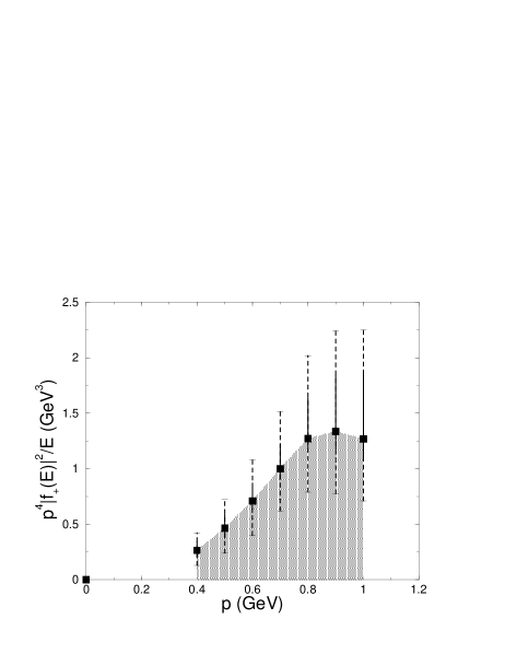
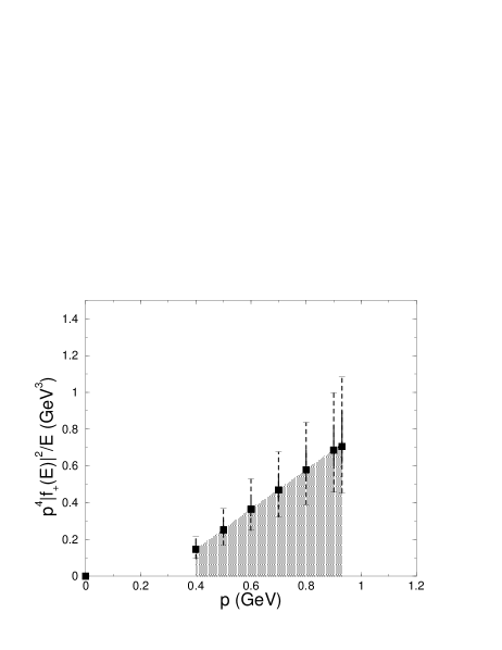
FIG. 1.: The differential decay rate (without momentum-independent factors) as a function of $p=|\mathchoice{{\hbox{\boldmath$\displaystyle p$}}}{{\hbox{\boldmath$\textstyle p$}}}{{\hbox{\boldmath$\scriptstyle p$}}}{{\hbox{\boldmath$\scriptscriptstyle p$}}}_{\pi}|$, for (a) $B\to\pi l\nu$ and (b) $D\to\pi l\nu$. The solid error bars show the statistical uncertainty and the dotted ones show the sum in quadrature of statistical and systematic uncertainties.

The shaded regions indicate the range of pion momentum over which we can control the uncertainties. Integrating over this region, we find

$$T_{B}(0.4~{}\text{GeV},1.0~{}\text{GeV}) = 0.55^{+\,0.15}_{-\,0.05}{\;}^{+\,0.09}_{-\,0.12}{\,}^{+\,0.09}_{-\,0.02}\pm 0.06\pm 0.09~{}\text{GeV}^{4},$$ (6)

$$T_{D}(0.4~{}\text{GeV},0.925~{}\text{GeV}) = 0.23^{+\,0.04}_{-\,0.02}{\;}^{+\,0.01}_{-\,0.05}{\,}^{+\,0.06}_{-\,0.02}\pm 0.03\pm 0.03~{}\text{GeV}^{4}.$$ (7)

where the first uncertainty is statistical, and following four are systematic and come from chiral extrapolation, lattice spacing dependence, matching to continuum QCD, and the sum in quadrature of several other uncertainties. The last includes an estimate of the uncertainty from converting lattice units to physical units, which partly reflects uncertainty from the quenched approximation. In addition to these uncertainties, which are quantifiable within the quenched approximation, there may be an additional error from quenching as large as 10–20 percent on $T_{B}$ and $T_{D}$.

At low momenta the experimental rates go to zero, so no information is lost by making the cut at $p_{\text{min}}=0.4$ GeV. For semileptonic $D$ decays the high-momentum cut is already at the kinematic endpoint $(m_{D}^{2}-m_{\pi}^{2})/2m_{D}=0.925$ GeV. A high-momentum cut at $p_{\text{max}}=1.0$ GeV is, however, an obstacle to determining $|V_{ub}|$, since semileptonic $B$ decays usually produce harder pions. Although the cut does reduce the overlap between our lattice calculation and experimental results, the results presented here are model independent (apart from quenching). As experimental and lattice results improve over the next several years, the range of pion momentum should widen and can be selected to optimize the combined experimental and theoretical uncertainty.

This paper is organized as follows. Section II contains a discussion of the lattice action and vector current for heavy quarks. The lattice calculation of the matrix elements is described in Sec. III. Section IV describes an interpolation in pion three-momentum and an extrapolation in light quark mass, which are needed to obtain the form factors. The former is a special feature of these decays; it interacts with the chiral limit, and together these lead to the cuts given in Eqs. (6) and (7). We discuss quantitatively the systematic errors on $T_{B}$ and $T_{D}$ in Sec. V. The analysis of $B$ and $D$ decays is essentially the same. Results for the form factors are tabulated in Sec. VI. Section VII compares our methods and results to previous (and ongoing) work [19, 20, 21]. Section VIII concludes.

Preliminary results of this analysis have been presented in Refs. [22, 23]. Phenomenological implications of $D$ decays, especially for comparing $D\to\pi l\nu$ and $D\to Kl\nu$ as in Ref. [24], will appear in another publication.

II Continuum and lattice matrix elements

The continuum matrix element of the flavor-changing vector current, ${\cal V}^{\mu}=\bar{u}i\gamma^{\mu}b$, is parametrized by two independent form factors, for example those in Eq. (2). In considering the chiral and heavy-quark limits, it is more convenient to write the matrix element as

$$\langle\pi(p_{\pi})|{\cal V}^{\mu}|B(p_{B})\rangle=\sqrt{2m_{B}}\left[v^{\mu}f_{\parallel}(E)+p^{\mu}_{\perp}f_{\perp}(E)\right],$$ (8)

where $v=p_{B}/m_{B}$ is the four-velocity of the $B$, and $p_{\perp}=p_{\pi}-Ev$ is the pion momentum orthogonal to $v$. The traditional form factors $f_{+}$ and $f_{0}$ are related to $f_{\parallel}$ and $f_{\perp}$ by

$$f_{+}(E) = (2m_{B})^{-1/2}\left[f_{\parallel}(E)+(m_{B}-E)f_{\perp}(E)\right],$$ (9)

$$f_{0}(E) = \frac{\sqrt{2m_{B}}}{m_{B}^{2}-m_{\pi}^{2}}\left[(m_{B}-E)f_{\parallel}(E)+(E^{2}-m_{\pi}^{2})f_{\perp}(E)\right].$$ (10)

At $q^{2}=0$ it follows from these formulae that $f_{+}=f_{0}$, which is necessary from Eq. (2).

There are several good reasons to focus the numerical analysis on $f_{\parallel}$ and $f_{\perp}$. First, consideration of chiral and heavy-quark symmetry yields the expectation for $m_{\pi}$, $E\to 0$

$$f_{\parallel} = \frac{f_{B}\sqrt{m_{B}}}{\sqrt{2}f_{\pi}},$$ (11)

$$f_{\perp} = \frac{f_{B^{*}}\sqrt{m_{B^{*}}}}{\sqrt{2}f_{\pi}}g_{BB^{*}\pi}\frac{2m_{B}}{m_{B^{*}}^{2}-q^{2}},$$ (12)

through order $1/m_{Q}$ in the heavy-quark expansion [25]. Here $f_{B}$, $f_{B^{*}}$, and $f_{\pi}$ are decay constants, and $g_{BB^{*}\pi}$ is the $B$-$B^{*}$-$\pi$ coupling. Although we do not use these results to constrain the needed chiral extrapolation of our data, they do show us that $f_{\parallel}$ and $f_{\perp}$ behave differently as $m_{\pi}$ is reduced to its physical value. (Recall $q^{2}=m_{B}^{2}+m_{\pi}^{2}-2m_{B}E$.) Furthermore, $f_{\parallel}$ and $f_{\perp}$ have a simple description in the heavy-quark effective theory [25], so they are natural quantities to study in the lattice method of Refs. [11, 12], or when using lattice NRQCD [21]. Finally, they emerge directly from the lattice calculation, so it is simpler to analyze them separately, forming the linear combinations in Eqs. (9) and (10) at the end.

For the light quarks we use the Sheikholeslami-Wohlert (SW) action [26], with the customary normalization conditions for $m_{q}a\to 0$. The SW action has an extra coupling $c_{\text{SW}}$, sometimes called the “clover” coupling, which can be adjusted to reduce the leading lattice-spacing effect of Wilson fermions. In practice, we adjust $c_{\text{SW}}$ according to tadpole-improved, tree-level perturbation theory [27], so the leading light-quark cutoff effect is of order $\alpha_{s}ka$.

We also use the SW action for the heavy quark, but its two free parameters, the bare mass $m_{0}$ and clover coupling $c_{\text{SW}}$, are adjusted to maintain good behavior in the heavy-quark limit [11]. This goes as follows: on-shell lattice matrix elements can be described by a version of HQET [12], with effective Lagrangian (in the rest frame)

$${\cal L}_{\text{HQET}}=m_{1}\bar{h}h+\frac{\bar{h}\mathchoice{{\hbox{\boldmath$\displaystyle D$}}}{{\hbox{\boldmath$\textstyle D$}}}{{\hbox{\boldmath$\scriptstyle D$}}}{{\hbox{\boldmath$\scriptscriptstyle D$}}}^{2}h}{2m_{2}}+\frac{\bar{h}\,i\mathchoice{{\hbox{\boldmath$\displaystyle\Sigma$}}}{{\hbox{\boldmath$\textstyle\Sigma$}}}{{\hbox{\boldmath$\scriptstyle\Sigma$}}}{{\hbox{\boldmath$\scriptscriptstyle\Sigma$}}}\cdot\mathchoice{{\hbox{\boldmath$\displaystyle B$}}}{{\hbox{\boldmath$\textstyle B$}}}{{\hbox{\boldmath$\scriptstyle B$}}}{{\hbox{\boldmath$\scriptscriptstyle B$}}}\,h}{2m_{\cal B}}+\cdots,$$ (13)

where $h$ is the heavy-quark field of HQET, and $\textstyle B$ is the chromomagnetic field. The “masses” $m_{1}$, $m_{2}$, and $m_{\cal B}$ are short-distance coefficients; they depend on $m_{0}$ and $c_{\text{SW}}$ (and the gauge coupling). Fortunately, matrix elements are completely independent of $m_{1}$ [12], so we adjust $m_{0}$ and $c_{\text{SW}}$ to tune $m_{2}$ and $m_{\cal B}$ to the $b$ (or $c$) quark. In practice, we tune $m_{2}$ non-perturbatively, using the quarkonium spectra, and $m_{\cal B}$ with the estimate of tadpole-improved, tree-level perturbation theory [27].

The lattice current is constructed according to the same principles. We distinguish the lattice current $V$ from its continuum counterpart ${\cal V}$ and take

$$V^{\mu}=\sqrt{Z_{V^{uu}}Z_{V^{bb}}}\bar{\Psi}_{u}i\gamma^{\mu}\Psi_{b}$$ (14)

where the rotated field [11]

$$\Psi_{q}=\left[1+ad_{1}\mathchoice{{\hbox{\boldmath$\displaystyle\gamma$}}}{{\hbox{\boldmath$\textstyle\gamma$}}}{{\hbox{\boldmath$\scriptstyle\gamma$}}}{{\hbox{\boldmath$\scriptscriptstyle\gamma$}}}\cdot\mathchoice{{\hbox{\boldmath$\displaystyle D$}}}{{\hbox{\boldmath$\textstyle D$}}}{{\hbox{\boldmath$\scriptstyle D$}}}{{\hbox{\boldmath$\scriptscriptstyle D$}}}_{\text{lat}}\right]\psi_{q},$$ (15)

and $\psi_{q}$ is the lattice quark field ($q=u,\;b$) in the SW action. Here $\mathchoice{{\hbox{\boldmath$\displaystyle D$}}}{{\hbox{\boldmath$\textstyle D$}}}{{\hbox{\boldmath$\scriptstyle D$}}}{{\hbox{\boldmath$\scriptscriptstyle D$}}}_{\text{lat}}$ is the symmetric, nearest-neighbor, covariant difference operator. In Eq. (14) the factors $Z_{V^{qq}}$, $q=u,b$, normalize the flavor-conserving currents. In practice, they are computed non-perturbatively.

Matching the current $V^{\mu}$ to HQET requires further short-distance coefficients:

$$V^{\mu}\doteq(\eta_{V}^{\text{lat}}+\zeta_{V}^{\text{lat}})v^{\mu}\bar{q}h+\eta_{V}^{\text{lat}}\bar{q}i\gamma^{\mu}_{\perp}h-\frac{\bar{q}i\gamma^{\mu}{\kern 1.00006pt/\kern-6.49994ptD}_{\perp}h}{2m_{3}}+\cdots,$$ (16)

where the symbol $\doteq$ implies equality of matrix elements, and $\bar{q}$ is a relativistic (continuum) anti-quark field. At the tree level $\eta_{V}^{\text{lat}}=1$, $\zeta_{V}^{\text{lat}}=0$. Also, further dimension-four operators, whose coefficients vanish at the tree level, are omitted from the right-hand side of Eq. (16). This description is in complete analogy with that for the continuum current, namely,

$${\cal V}^{\mu}\doteq(\eta_{V}+\zeta_{V})v^{\mu}\bar{q}h+\eta_{V}\bar{q}i\gamma^{\mu}_{\perp}h-\frac{B_{1}\bar{q}i\gamma^{\mu}{\kern 1.00006pt/\kern-6.49994ptD}_{\perp}h}{2m_{Q}}+\cdots.$$ (17)

Indeed, the HQET operators are the same. On the other hand, the radiative corrections to the short-distance coefficients in Eqs. (16) and Eqs. (17) differ, because the lattice modifies the physics at short distances.

By studying the form factors in HQET, as in Ref. [25], one can deduce how to compensate for the mismatch between short-distance coefficients $\eta_{V}^{\text{(lat)}}$ and $\zeta_{V}^{\text{(lat)}}$ for the lattice and $\eta_{V}$ and $\zeta_{V}$ for the continuum. HQET matrix elements have form factors

$$\langle\pi|\bar{q}h|B\rangle = \varphi_{\parallel}(E),$$ (18)

$$\langle\pi|\bar{q}i\gamma_{\perp}^{\mu}h|B\rangle = p_{\perp}^{\mu}\varphi_{\perp}(E),$$ (19)

so, leaving aside the dimension-four operator $\bar{q}i\gamma^{\mu}{\kern 1.00006pt/\kern-6.49994ptD}_{\perp}h$ for now,

$$f_{\parallel}(E) = \eta_{V}\varphi_{\parallel}(E),$$ (20)

$$f_{\perp}(E) = (\eta_{V}+\zeta_{V})\varphi_{\perp}(E).$$ (21)

By the same reasoning, form factors calculated with the lattice current $V$ satisfy

$$f^{\text{lat}}_{\parallel}(E) = \eta^{\text{lat}}_{V}\varphi_{\parallel}(E),$$ (22)

$$f^{\text{lat}}_{\perp}(E) = (\eta^{\text{lat}}_{V}+\zeta^{\text{lat}}_{V})\varphi_{\perp}(E).$$ (23)

Up to lattice artifacts of the light degrees of freedom the HQET form factors $\varphi_{\parallel}$ and $\varphi_{\perp}$ are the same in Eqs. (20) and (21) and in Eqs. (22) and (23). Thus,

$$f_{\parallel}(E) = \rho_{V_{\parallel}}f^{\text{lat}}_{\parallel}(E),$$ (24)

$$f_{\perp}(E) = \rho_{V_{\perp}}f^{\text{lat}}_{\perp}(E),$$ (25)

where $\rho_{V_{\parallel}}=\eta_{V}/\eta^{\text{lat}}_{V}$, $\rho_{V_{\perp}}=(\eta_{V}+\zeta_{V})/(\eta^{\text{lat}}_{V}+\zeta^{\text{lat}}_{V})$. Because these factors arise from short distances, in practice we compute them in perturbation theory to one loop. We find these short-distance corrections to be very small.

Finally, the free parameter $d_{1}$ in Eq. (15) can be adjusted to tune $1/m_{3}$ to $B_{1}/m_{Q}$. In the present calculations, we adjust $d_{1}$ with the estimate of tadpole-improved, tree-level perturbation theory, as explained in Ref. [11].

With these normalization conditions the leading term in the heavy-quark expansion is correctly obtained, up to neglected higher-order corrections to $\rho_{V_{\parallel}}$ and $\rho_{V_{\perp}}$. The associated error should be much smaller than our other uncertainties, because most of the short-distance normalization is handled non-perturbatively, through the factor $\sqrt{Z_{V^{uu}}Z_{V^{bb}}}$. Similarly, the $1/m_{Q}$ term in the heavy-quark expansion is correctly obtained, up to neglected loop corrections to $c_{\text{SW}}$ and $d_{1}$, and to dimension-four operators neglected in Eq. (16). Here the associated error depends on $m_{Q}a$. When $m_{Q}a>1$ it is formally of order $\alpha_{s}\Lambda_{\text{QCD}}/m_{Q}$, but when $m_{Q}a<1$ it is formally of order $\alpha_{s}\Lambda_{\text{QCD}}a$. In the work reported here, such corrections are smaller than, or comparable to, other uncertainties.

In lattice QCD the required matrix elements and thence the form factors are calculated from correlation functions. In particular, the three-point correlation function for the $B\to\pi$ transition is

$$C_{\mu}^{(3)}(\mathchoice{{\hbox{\boldmath$\displaystyle p$}}}{{\hbox{\boldmath$\textstyle p$}}}{{\hbox{\boldmath$\scriptstyle p$}}}{{\hbox{\boldmath$\scriptscriptstyle p$}}},\mathchoice{{\hbox{\boldmath$\displaystyle k$}}}{{\hbox{\boldmath$\textstyle k$}}}{{\hbox{\boldmath$\scriptstyle k$}}}{{\hbox{\boldmath$\scriptscriptstyle k$}}},t_{f},t_{s},t_{i})=\sum_{\mathchoice{{\hbox{\boldmath$\displaystyle x$}}}{{\hbox{\boldmath$\textstyle x$}}}{{\hbox{\boldmath$\scriptstyle x$}}}{{\hbox{\boldmath$\scriptscriptstyle x$}}},\mathchoice{{\hbox{\boldmath$\displaystyle y$}}}{{\hbox{\boldmath$\textstyle y$}}}{{\hbox{\boldmath$\scriptstyle y$}}}{{\hbox{\boldmath$\scriptscriptstyle y$}}}}e^{-i\mathchoice{{\hbox{\boldmath$\displaystyle p$}}}{{\hbox{\boldmath$\textstyle p$}}}{{\hbox{\boldmath$\scriptstyle p$}}}{{\hbox{\boldmath$\scriptscriptstyle p$}}}\cdot\mathchoice{{\hbox{\boldmath$\displaystyle x$}}}{{\hbox{\boldmath$\textstyle x$}}}{{\hbox{\boldmath$\scriptstyle x$}}}{{\hbox{\boldmath$\scriptscriptstyle x$}}}}e^{-i(\mathchoice{{\hbox{\boldmath$\displaystyle k$}}}{{\hbox{\boldmath$\textstyle k$}}}{{\hbox{\boldmath$\scriptstyle k$}}}{{\hbox{\boldmath$\scriptscriptstyle k$}}}-\mathchoice{{\hbox{\boldmath$\displaystyle p$}}}{{\hbox{\boldmath$\textstyle p$}}}{{\hbox{\boldmath$\scriptstyle p$}}}{{\hbox{\boldmath$\scriptscriptstyle p$}}})\cdot\mathchoice{{\hbox{\boldmath$\displaystyle y$}}}{{\hbox{\boldmath$\textstyle y$}}}{{\hbox{\boldmath$\scriptstyle y$}}}{{\hbox{\boldmath$\scriptscriptstyle y$}}}}\langle 0|{\cal O}_{B}(\mathchoice{{\hbox{\boldmath$\displaystyle x$}}}{{\hbox{\boldmath$\textstyle x$}}}{{\hbox{\boldmath$\scriptstyle x$}}}{{\hbox{\boldmath$\scriptscriptstyle x$}}},t_{f})\bar{\Psi}_{b}\gamma_{\mu}\Psi_{u}(\mathchoice{{\hbox{\boldmath$\displaystyle y$}}}{{\hbox{\boldmath$\textstyle y$}}}{{\hbox{\boldmath$\scriptstyle y$}}}{{\hbox{\boldmath$\scriptscriptstyle y$}}},t_{s}){\cal O}^{\dagger}_{\pi}(\mathchoice{{\hbox{\boldmath$\displaystyle 0$}}}{{\hbox{\boldmath$\textstyle 0$}}}{{\hbox{\boldmath$\scriptstyle 0$}}}{{\hbox{\boldmath$\scriptscriptstyle 0$}}},t_{i})|0\rangle,$$ (26)

where ${\cal O}_{B}$ and ${\cal O}_{\pi}$ are interpolating operators for the $B$ and $\pi$ mesons. In the limit of large time separations, the correlation function becomes

$$C_{\mu}^{(3)}(\mathchoice{{\hbox{\boldmath$\displaystyle p$}}}{{\hbox{\boldmath$\textstyle p$}}}{{\hbox{\boldmath$\scriptstyle p$}}}{{\hbox{\boldmath$\scriptscriptstyle p$}}},\mathchoice{{\hbox{\boldmath$\displaystyle k$}}}{{\hbox{\boldmath$\textstyle k$}}}{{\hbox{\boldmath$\scriptstyle k$}}}{{\hbox{\boldmath$\scriptscriptstyle k$}}},t_{f},t_{s},t_{i})={\cal Z}_{B}^{1/2}{\cal Z}_{\pi}^{1/2}\frac{\langle B(\mathchoice{{\hbox{\boldmath$\displaystyle k$}}}{{\hbox{\boldmath$\textstyle k$}}}{{\hbox{\boldmath$\scriptstyle k$}}}{{\hbox{\boldmath$\scriptscriptstyle k$}}})|\bar{\Psi}_{b}\gamma_{\mu}\Psi_{u}|\pi(\mathchoice{{\hbox{\boldmath$\displaystyle p$}}}{{\hbox{\boldmath$\textstyle p$}}}{{\hbox{\boldmath$\scriptstyle p$}}}{{\hbox{\boldmath$\scriptscriptstyle p$}}})\rangle}{\sqrt{2E_{B}}\hfil\sqrt{2E_{\pi}}}e^{-E_{\pi}(t_{s}-t_{i})}e^{-E_{B}(t_{f}-t_{s})}+\cdots,$$ (27)

where $E_{B}$ ($E_{\pi}$) is the energy of a $B$ ($\pi$) meson with momentum $\textstyle k$ ($\textstyle p$). The energies and the external line factors ${\cal Z}_{\pi}$ and ${\cal Z}_{B}$ can be calculated from two-point correlation functions

$$C^{(2)}(\mathchoice{{\hbox{\boldmath$\displaystyle p$}}}{{\hbox{\boldmath$\textstyle p$}}}{{\hbox{\boldmath$\scriptstyle p$}}}{{\hbox{\boldmath$\scriptscriptstyle p$}}},t)=\sum_{\mathchoice{{\hbox{\boldmath$\displaystyle x$}}}{{\hbox{\boldmath$\textstyle x$}}}{{\hbox{\boldmath$\scriptstyle x$}}}{{\hbox{\boldmath$\scriptscriptstyle x$}}}}e^{-i\mathchoice{{\hbox{\boldmath$\displaystyle p$}}}{{\hbox{\boldmath$\textstyle p$}}}{{\hbox{\boldmath$\scriptstyle p$}}}{{\hbox{\boldmath$\scriptscriptstyle p$}}}\cdot\mathchoice{{\hbox{\boldmath$\displaystyle x$}}}{{\hbox{\boldmath$\textstyle x$}}}{{\hbox{\boldmath$\scriptstyle x$}}}{{\hbox{\boldmath$\scriptscriptstyle x$}}}}\langle 0|{\cal O}_{H}(\mathchoice{{\hbox{\boldmath$\displaystyle x$}}}{{\hbox{\boldmath$\textstyle x$}}}{{\hbox{\boldmath$\scriptstyle x$}}}{{\hbox{\boldmath$\scriptscriptstyle x$}}},t){\cal O}^{\dagger}_{H}(\mathchoice{{\hbox{\boldmath$\displaystyle 0$}}}{{\hbox{\boldmath$\textstyle 0$}}}{{\hbox{\boldmath$\scriptstyle 0$}}}{{\hbox{\boldmath$\scriptscriptstyle 0$}}},0)|0\rangle,$$ (28)

where $H$ is $\pi$ or $B$, and for large $|t|$ one has

$$C^{(2)}(\mathchoice{{\hbox{\boldmath$\displaystyle p$}}}{{\hbox{\boldmath$\textstyle p$}}}{{\hbox{\boldmath$\scriptstyle p$}}}{{\hbox{\boldmath$\scriptscriptstyle p$}}},t)={\cal Z}_{H}e^{-E_{H}|t|}+\cdots.$$ (29)

By time reversal $\langle B(\mathchoice{{\hbox{\boldmath$\displaystyle k$}}}{{\hbox{\boldmath$\textstyle k$}}}{{\hbox{\boldmath$\scriptstyle k$}}}{{\hbox{\boldmath$\scriptscriptstyle k$}}})|\bar{\Psi}_{b}\gamma_{\mu}\Psi_{u}|\pi(\mathchoice{{\hbox{\boldmath$\displaystyle p$}}}{{\hbox{\boldmath$\textstyle p$}}}{{\hbox{\boldmath$\scriptstyle p$}}}{{\hbox{\boldmath$\scriptscriptstyle p$}}})\rangle=\langle\pi(\mathchoice{{\hbox{\boldmath$\displaystyle p$}}}{{\hbox{\boldmath$\textstyle p$}}}{{\hbox{\boldmath$\scriptstyle p$}}}{{\hbox{\boldmath$\scriptscriptstyle p$}}})|\bar{\Psi}_{u}\gamma_{\mu}\Psi_{b}|B(\mathchoice{{\hbox{\boldmath$\displaystyle k$}}}{{\hbox{\boldmath$\textstyle k$}}}{{\hbox{\boldmath$\scriptstyle k$}}}{{\hbox{\boldmath$\scriptscriptstyle k$}}})\rangle$, so in the rest of this paper we do not distinguish the two matrix elements.

To summarize this section, let us review the steps needed to obtain the physical form factors $f_{+}$ and $f_{0}$. First we obtain $E_{\pi}$ and

$$F_{\parallel}(\mathchoice{{\hbox{\boldmath$\displaystyle p$}}}{{\hbox{\boldmath$\textstyle p$}}}{{\hbox{\boldmath$\scriptstyle p$}}}{{\hbox{\boldmath$\scriptscriptstyle p$}}}) = \frac{\langle B(\mathchoice{{\hbox{\boldmath$\displaystyle 0$}}}{{\hbox{\boldmath$\textstyle 0$}}}{{\hbox{\boldmath$\scriptstyle 0$}}}{{\hbox{\boldmath$\scriptscriptstyle 0$}}})|\bar{\Psi}_{b}\gamma_{4}\Psi_{u}|\pi(\mathchoice{{\hbox{\boldmath$\displaystyle p$}}}{{\hbox{\boldmath$\textstyle p$}}}{{\hbox{\boldmath$\scriptstyle p$}}}{{\hbox{\boldmath$\scriptscriptstyle p$}}})\rangle}{\sqrt{2m_{B}}\hfil\sqrt{2E_{\pi}}},$$ (30)

$$F_{\perp}(\mathchoice{{\hbox{\boldmath$\displaystyle p$}}}{{\hbox{\boldmath$\textstyle p$}}}{{\hbox{\boldmath$\scriptstyle p$}}}{{\hbox{\boldmath$\scriptscriptstyle p$}}}) = \frac{1}{p_{j}a}\frac{\langle B(\mathchoice{{\hbox{\boldmath$\displaystyle 0$}}}{{\hbox{\boldmath$\textstyle 0$}}}{{\hbox{\boldmath$\scriptstyle 0$}}}{{\hbox{\boldmath$\scriptscriptstyle 0$}}})|\bar{\Psi}_{b}\gamma_{j}\Psi_{u}|\pi(\mathchoice{{\hbox{\boldmath$\displaystyle p$}}}{{\hbox{\boldmath$\textstyle p$}}}{{\hbox{\boldmath$\scriptstyle p$}}}{{\hbox{\boldmath$\scriptscriptstyle p$}}})\rangle}{\sqrt{2m_{B}}\hfil\sqrt{2E_{\pi}}},$$ (31)

for several values of $\textstyle p$, directly from fitting the lattice correlation functions to the time dependence given in Eqs. (27) and (29). The normalization factors $Z_{V^{uu}}$ and $Z_{V^{bb}}$ are computed from zero-momentum, flavor-conserving correlation functions. The radiative correction factors $\rho_{V}$ appearing in Eqs. (24) and (25) are computed with perturbation theory. These ingredients are combined to form

$$f_{\parallel}(E) = \rho_{V_{\parallel}}\sqrt{Z_{V^{uu}}Z_{V^{bb}}}\sqrt{2E_{\pi}}\,F_{\parallel}(\mathchoice{{\hbox{\boldmath$\displaystyle p$}}}{{\hbox{\boldmath$\textstyle p$}}}{{\hbox{\boldmath$\scriptstyle p$}}}{{\hbox{\boldmath$\scriptscriptstyle p$}}}),$$ (32)

$$f_{\perp}(E) = \rho_{V_{\perp}}\sqrt{Z_{V^{uu}}Z_{V^{bb}}}\sqrt{2E_{\pi}}\,aF_{\perp}(\mathchoice{{\hbox{\boldmath$\displaystyle p$}}}{{\hbox{\boldmath$\textstyle p$}}}{{\hbox{\boldmath$\scriptstyle p$}}}{{\hbox{\boldmath$\scriptscriptstyle p$}}}),$$ (33)

with $E=E_{\pi}$. From the calculated values of $\textstyle p$ we then interpolate to a fiducial set of momenta. The form factors $f_{\parallel}$ and $f_{\perp}$ are extrapolated to the physical light quark mass. With the light quark corresponding to strange we check also for lattice spacing effects. Finally, the combinations $f_{+}$ and $f_{0}$ are formed from the extrapolated $f_{\perp}$ and $f_{\parallel}$ with Eqs. (9) and (10) and physical meson masses.

III Lattice calculation

This work uses three ensembles of lattice gauge field configurations, which have been used in previous work on heavy-light decay constants [28, 14], light-quark masses [29], and quarkonia [30]. The quark propagators are the same as in Ref. [14], but we now use 200 instead of 100 configurations on the finest lattice (with $\beta=6.1$). The input parameters for these fields are in Table I, together with some elementary output parameters.

TABLE I.: Input parameters to the numerical lattice calculations, together with some elementary output parameters. Error bars on the outputs refer to the last digit(s).

Inputs
$\beta=6/g_{0}^{2}$	6.1	5.9	5.7
Volume, $N_{S}^{3}\times N_{T}$	$24^{3}\times 48$	$16^{3}\times 32$	$12^{3}\times 24$
Configurations	200	350	300
$c_{\rm sw}$	1.46	1.50	1.57
$\kappa_{b}$, $m_{0}$ (GeV)	0.0990, 4.31	0.0930, 3.73	0.0890, 2.87
$\kappa_{c}$, $m_{0}$ (GeV)	0.1260, 1.07	0.1227, 1.05	0.1190, 0.96
$\kappa_{s}$, $m_{0}$ (GeV)	0.1373, 0.092	0.1385, 0.091	0.1405, 0.093
$\kappa_{q}$, $m_{0}$ (GeV)		0.1382, 0.107
		0.1388, 0.075	0.1410, 0.076
		0.1391, 0.059	0.1415, 0.059
		0.1394, 0.043	0.1419, 0.045
Elementary outputs
$\kappa_{\text{crit}}$	0.13847$\;\begin{array}[]{@{}l@{}}\makebox[15.0pt][c]{$+$}\makebox[2.5pt][r]{4\hfill}\\[-1.19995pt] \makebox[15.0pt][c]{$-$}\makebox[2.5pt][r]{2\hfill}\end{array}$	0.14021$\;\begin{array}[]{@{}l@{}}\makebox[15.0pt][c]{$+$}\makebox[2.5pt][r]{3\hfill}\\[-1.19995pt] \makebox[15.0pt][c]{$-$}\makebox[2.5pt][r]{1\hfill}\end{array}$	0.14327$\;\begin{array}[]{@{}l@{}}\makebox[15.0pt][c]{$+$}\makebox[2.5pt][r]{5\hfill}\\[-1.19995pt] \makebox[15.0pt][c]{$-$}\makebox[2.5pt][r]{2\hfill}\end{array}$
$a^{-1}_{\text{1P-1S}}$ (GeV)	2.64$\;\begin{array}[]{@{}l@{}}\makebox[15.0pt][c]{$+$}\makebox[5.0pt][r]{17\hfill}\\[-2.40005pt] \makebox[15.0pt][c]{$-$}\makebox[5.0pt][r]{13\hfill}\end{array}$	1.80$\;\begin{array}[]{@{}l@{}}\makebox[15.0pt][c]{$+$}\makebox[2.5pt][r]{7\hfill}\\[-1.19995pt] \makebox[15.0pt][c]{$-$}\makebox[2.5pt][r]{6\hfill}\end{array}$	1.16$\;\begin{array}[]{@{}l@{}}\makebox[15.0pt][c]{$+$}\makebox[2.5pt][r]{3\hfill}\\[-1.19995pt] \makebox[15.0pt][c]{$-$}\makebox[2.5pt][r]{3\hfill}\end{array}$
$a^{-1}_{f_{\pi}}$ (GeV)	2.40$\;\begin{array}[]{@{}l@{}}\makebox[15.0pt][c]{$+$}\makebox[5.0pt][r]{10\hfill}\\[-2.40005pt] \makebox[15.0pt][c]{$-$}\makebox[5.0pt][r]{12\hfill}\end{array}$	1.47$\;\begin{array}[]{@{}l@{}}\makebox[15.0pt][c]{$+$}\makebox[2.5pt][r]{6\hfill}\\[-1.19995pt] \makebox[15.0pt][c]{$-$}\makebox[2.5pt][r]{6\hfill}\end{array}$	0.89$\;\begin{array}[]{@{}l@{}}\makebox[15.0pt][c]{$+$}\makebox[2.5pt][r]{2\hfill}\\[-1.19995pt] \makebox[15.0pt][c]{$-$}\makebox[2.5pt][r]{2\hfill}\end{array}$
$2\pi/N_{S}a$ (GeV)	0.686	0.707	0.607
$u_{0}$	0.8816	0.8734	0.8608
$\alpha_{V}(2/a)$	0.171	0.192	0.227

The quark propagators are computed from the Sheikholeslami-Wohlert action, which includes a dimension-five interaction with coupling $c_{\text{SW}}$. For heavy and light quarks we adjust $c_{\text{SW}}$ to the value $u_{0}^{-3}$ suggested by tadpole-improved, tree-level perturbation theory, and the so-called mean link $u_{0}$ is calculated from the plaquette. The hopping parameter $\kappa$ is related to the bare quark mass. For bottom and charmed quarks, $\kappa_{b}$ and $\kappa_{c}$ are adjusted so that the spin-averaged kinetic mass of the corresponding 1S quarkonium states match experimental measurements. For light quarks, $\kappa_{s}$ and $\kappa_{q}$ are fixed from light meson spectroscopy, using leading-order chiral perturbation theory and the experimental kaon and pion masses. We also list the tadpole-improved bare quark mass in GeV,

$$m_{0}a=\frac{1}{u_{0}}\left(\frac{1}{2\kappa}-\frac{1}{2\kappa_{\text{crit}}}\right),$$ (34)

where the critical quark hopping parameter $\kappa_{\text{crit}}$ makes the pion massless. Although this mass is just a bare mass, it shows that the heavy quarks are heavy, and the light quarks light.

We calculate the three-point function in Eq. (27) with degenerate spectator and daughter light quarks. At each lattice spacing we have propagators corresponding to the strange quark. We refer to this decay as $B_{s}\to\eta_{s}l\nu$, writing $\eta_{s}$ for the pseudoscalar $\bar{s}s$ state in analogy with quarkonium. At $\beta=5.9$ and $5.7$ we have additional light quark propagators, with hopping parameter $\kappa_{q}$, covering the range $\frac{1}{2}m_{s}\lesssim m_{q}\lesssim m_{s}$.

The lattice spacing $a$ in physical units must be set through some fiducial observable. As a rule [30] we prefer the spin-averaged 1P-1S splitting of charmonium, $\Delta m_{\text{1P-1S}}$. For comparison we give the value of $a^{-1}$ defined through the pion decay constant $f_{\pi}$. The discrepancy means that $\Delta m_{\text{1P-1S}}/f_{\pi}$ does not agree with experiment; this is thought to be largely due to the quenched approximation, because it remains even as $a$ is decreased.

The renormalized strong coupling $\alpha_{V}(2/a)$ at scale $2/a$ is determined as in Ref. [27]. It is an ingredient in the calculation of the short-distance coefficients $\rho_{V_{\parallel}}$ and $\rho_{V_{\perp}}$, introduced in Eqs. (24) and (25).

In the three-point functions the heavy-light meson is at rest, while the momentum of the light daughter meson is varied. In a finite volume only discrete values of spatial momentum are accessible. We compute the three-point function with $\mathchoice{{\hbox{\boldmath$\displaystyle p$}}}{{\hbox{\boldmath$\textstyle p$}}}{{\hbox{\boldmath$\scriptstyle p$}}}{{\hbox{\boldmath$\scriptscriptstyle p$}}}_{\pi}=2\pi\mathchoice{{\hbox{\boldmath$\displaystyle n$}}}{{\hbox{\boldmath$\textstyle n$}}}{{\hbox{\boldmath$\scriptstyle n$}}}{{\hbox{\boldmath$\scriptscriptstyle n$}}}/N_{S}a$, for integer momentum $\mathchoice{{\hbox{\boldmath$\displaystyle n$}}}{{\hbox{\boldmath$\textstyle n$}}}{{\hbox{\boldmath$\scriptstyle n$}}}{{\hbox{\boldmath$\scriptscriptstyle n$}}}\in\{(0,0,0),\,(1,0,0),\,(1,1,0),\,(1,1,1),\,(2,0,0)\}$. As one can see in Table I, one unit of momentum is about 0.7 GeV in the boxes used here, so our calculations cover the range $0\leq p<1.5$ GeV.

We obtain the energies, matrix elements, and ${\cal Z}_{H}$ factors by fitting Eqs. (27) and (29) with a $\chi^{2}$-minimization algorithm. Statistical errors, including the full correlation matrix in $\chi^{2}$, are determined from 1000 bootstrap samples for each best fit. The bootstrap procedure is repeated with the same sequence for all quark mass combinations and momenta, and in this way the fully correlated statistical errors are propagated through later stages of the analysis.

The right-hand sides of Eqs. (27) and (29) are the first term in a series, with another term for each radial excitation. We reduce contamination from these states two ways. First, we keep the three points of the three-point function well separated in (Euclidean) time. The light meson creation operator ${\cal O}_{\pi}$ is always at $t_{i}=0$ and the heavy-light meson annihilation operator at $t_{f}=N_{T}/2$. We then vary the time $t_{s}$ of the current and the range $\Delta t$ of time-slices kept in the fit, to see when the lowest-lying states dominate. The final choice is made by demanding that $\chi^{2}/\text{d.o.f.}$ is acceptable and, then, minimizing the statistical errors while maximizing $\Delta t$. For acceptable fits we have $3\leq\Delta t\leq 6$. The extraction of the desired matrix elements is shown in Fig. 2 for several light-meson momenta and typical quark mass. The best fit and error envelope are indicated by the solid and dotted lines respectively.

FIG. 2.: Matrix elements $F_{\parallel}$ (squares) and $F_{\perp}$ (diamonds) at $\beta=5.9$, for a light strange quark and a heavy bottom quark. The integer momenta are (a) $\mathchoice{{\hbox{\boldmath$\displaystyle n$}}}{{\hbox{\boldmath$\textstyle n$}}}{{\hbox{\boldmath$\scriptstyle n$}}}{{\hbox{\boldmath$\scriptscriptstyle n$}}}=(0,0,0)$, (b) $\mathchoice{{\hbox{\boldmath$\displaystyle n$}}}{{\hbox{\boldmath$\textstyle n$}}}{{\hbox{\boldmath$\scriptstyle n$}}}{{\hbox{\boldmath$\scriptscriptstyle n$}}}=(1,0,0)$, (c) $\mathchoice{{\hbox{\boldmath$\displaystyle n$}}}{{\hbox{\boldmath$\textstyle n$}}}{{\hbox{\boldmath$\scriptstyle n$}}}{{\hbox{\boldmath$\scriptscriptstyle n$}}}=(1,1,0)$, and (d) $\mathchoice{{\hbox{\boldmath$\displaystyle n$}}}{{\hbox{\boldmath$\textstyle n$}}}{{\hbox{\boldmath$\scriptstyle n$}}}{{\hbox{\boldmath$\scriptscriptstyle n$}}}=(1,1,1)$.

The second way to isolate the lowest-lying states is to choose interpolating operators, ${\cal O}_{B}$ and ${\cal O}_{\pi}$ in Eq. (26), to have a large overlap with the desired state. This is done by smearing out the quark and anti-quark with 1S and 2S Coulomb-gauge wave functions, as in Ref. [31]. We also examine point-like, or $\delta$ function, operators, but for light mesons at higher momenta we find that the $\delta$ source does not yield good plateaus [32]. The different combinations of sources and sinks allow us to check explicitly for excited state contributions by comparing results from fits with different smearing functions. Figure 3 compares results for the matrix element $\langle B_{s}|V^{\dagger}_{\mu}|\eta_{s}\rangle$ at $\mathchoice{{\hbox{\boldmath$\displaystyle n$}}}{{\hbox{\boldmath$\textstyle n$}}}{{\hbox{\boldmath$\scriptstyle n$}}}{{\hbox{\boldmath$\scriptscriptstyle n$}}}=(1,1,0)$, obtained from 1S source and sink and from 1S source for the light meson and $\delta$ sink for the $B_{s}$.

FIG. 3.: Isolation of the lowest-lying states with different smearing functions, for $\mathchoice{{\hbox{\boldmath$\displaystyle n$}}}{{\hbox{\boldmath$\textstyle n$}}}{{\hbox{\boldmath$\scriptstyle n$}}}{{\hbox{\boldmath$\scriptscriptstyle n$}}}=(1,1,0)$ and quark masses as in Fig. 2. The solid symbols have the standard 1S source and 1S sink; the open symbols have a $\delta$-function sink for the $B_{s}$.

The 1S-1S correlation functions yield the cleanest matrix elements, so we take our central values from them.

IV Analysis of form factors

From the exponential fits to three-point correlation functions described in Sec. III we have the matrix element, $\langle\eta_{q}(\mathchoice{{\hbox{\boldmath$\displaystyle p$}}}{{\hbox{\boldmath$\textstyle p$}}}{{\hbox{\boldmath$\scriptstyle p$}}}{{\hbox{\boldmath$\scriptscriptstyle p$}}})|V^{\mu}|B_{q}(\mathchoice{{\hbox{\boldmath$\displaystyle 0$}}}{{\hbox{\boldmath$\textstyle 0$}}}{{\hbox{\boldmath$\scriptstyle 0$}}}{{\hbox{\boldmath$\scriptscriptstyle 0$}}})\rangle$, for quark masses $m_{q}\lesssim m_{s}$ and final-state momenta $|\mathchoice{{\hbox{\boldmath$\displaystyle p$}}}{{\hbox{\boldmath$\textstyle p$}}}{{\hbox{\boldmath$\scriptstyle p$}}}{{\hbox{\boldmath$\scriptscriptstyle p$}}}|<1.4$ GeV. We must now extend these data to lower quark mass, until the mass of the $\bar{q}q$ pseudoscalar reaches the pion mass. Furthermore, the more important form factor $f_{\perp}(E)$, which is essentially $\langle\eta_{q}(\mathchoice{{\hbox{\boldmath$\displaystyle p$}}}{{\hbox{\boldmath$\textstyle p$}}}{{\hbox{\boldmath$\scriptstyle p$}}}{{\hbox{\boldmath$\scriptscriptstyle p$}}})|V_{j}|B_{q}(\mathchoice{{\hbox{\boldmath$\displaystyle 0$}}}{{\hbox{\boldmath$\textstyle 0$}}}{{\hbox{\boldmath$\scriptstyle 0$}}}{{\hbox{\boldmath$\scriptscriptstyle 0$}}})\rangle/p_{j}$, is directly calculated only for non-zero three-momentum. In the finite volume used here, the lowest non-zero momentum is already $0.7$ GeV, and we would like to extend to lower values, calling for another extrapolation.

The extrapolation in quark mass can be guided by chiral perturbation theory. To extrapolate in momentum, however, there is no firm theoretical guide, so we must exercise caution. Fortunately, this extrapolation is problematic only in the kinematic regime where phase space suppresses the rate. Consequently, neither extrapolation introduces a model. We also have checked that the order in which the momentum and chiral extrapolations are done has no significant effect the final result.

A Momentum interpolation and extrapolation

Ultimately, we want to compare results at the three different lattice spacings. Therefore, we interpolate the lattice data to a fixed set of physical momenta. To start, we convert the lattice data to physical units using $a^{-1}_{\text{1P-1S}}$. Figure 4 shows the underlying data for $B_{s}\to\eta_{s}l\nu$ at $\beta=5.9$ and $6.1$, along with interpolated points.

FIG. 4.: Momentum interpolation (and extrapolation) of $f_{\parallel}a^{+1/2}$ (squares) and $f_{\perp}a^{-1/2}$ (diamonds) for $B_{s}\to\eta_{s}l\nu$ at (a) $\beta=5.9$, (b) $\beta=6.1$. The solid points are the underlying data; the asterisks are interpolated.

The vertical (horizontal) error bars on the underlying data come from the statistical uncertainty in $F_{\parallel,\perp}$ ($a^{-1}$). We interpolate $\log f_{\perp}a^{-1/2}$ ($\log f_{\parallel}a^{+1/2}$) linearly (quadratically) in $\mathchoice{{\hbox{\boldmath$\displaystyle p$}}}{{\hbox{\boldmath$\textstyle p$}}}{{\hbox{\boldmath$\scriptstyle p$}}}{{\hbox{\boldmath$\scriptscriptstyle p$}}}^{2}$ to $|\mathchoice{{\hbox{\boldmath$\displaystyle p$}}}{{\hbox{\boldmath$\textstyle p$}}}{{\hbox{\boldmath$\scriptstyle p$}}}{{\hbox{\boldmath$\scriptscriptstyle p$}}}|\in\{0,0.1,0.2,0.3,0.4,0.5,0.6,0.7,0.8,0.9,1.0,1.1\}$ GeV. This set forms the basis of all further analysis. The statistical error bars of the interpolated points are vertical only, because both statistical errors are propagated through the interpolation.

We must extend the interpolation to an extrapolation to obtain an estimate of $f_{\perp}$ for $p<0.7$ GeV. As the pion becomes softer and lighter one expects from Eq. (12) that the dependence on $E$ (and hence $p$) is sensitive to the Ansatz for extrapolation. The $B^{*}$ pole gives $f_{\perp}$ a peak at low momentum, and the height of the peak rises as the quark mass decreases. This shape is hard to capture, as is shown in Fig. 5, unless the fit is constrained to it.

FIG. 5.: Momentum interpolation (and extrapolation) at $\beta=5.9$, for $B_{q}\to\eta_{q}l\nu$ and (a) the heaviest of our light quarks, with $\kappa_{q}=0.1382$; (b) the lightest of the light quarks, with $\kappa_{q}=0.1394$.

For $p>0.7$ GeV the pole fit agrees perfectly with the method described above. But as $p$ is decreased into the region of extrapolation, the two forms start to deviate. Above 0.4 GeV the agreement is still good, so we make a cut here. For smaller momenta phase space suppresses the number of events, so this cut has no serious ramifications. For $D$ decays the situation is much the same, as shown in Fig. 6.

FIG. 6.: Momentum interpolation (and extrapolation) at $\beta=5.9$, for $D_{q}\to\eta_{q}l\nu$ and (a) the heaviest of our light quarks, with $\kappa_{q}=0.1382$; (b) the lightest of the light quarks, with $\kappa_{q}=0.1394$.

Therefore, we impose the same low-momentum cut in this case. Other functional forms, such as rational, do not make much difference in $d\Gamma/dp\propto p^{4}|f_{+}|^{2}/E$, once the cut at $p_{\text{min}}=0.4$ GeV is imposed.

At high momentum there are other difficulties. The signal-to-noise ratio of the three-point function deteriorates. For the highest momentum, $\mathchoice{{\hbox{\boldmath$\displaystyle n$}}}{{\hbox{\boldmath$\textstyle n$}}}{{\hbox{\boldmath$\scriptstyle n$}}}{{\hbox{\boldmath$\scriptscriptstyle n$}}}=(2,0,0)$, we cannot always extract a convincing matrix element: in some cases the plateau $\Delta t$ is just 2 time-slices, and three-point functions with different sources and sinks do not yield the same value for the matrix element. We cannot include these data in the interpolation. For the second-highest momentum, $\mathchoice{{\hbox{\boldmath$\displaystyle n$}}}{{\hbox{\boldmath$\textstyle n$}}}{{\hbox{\boldmath$\scriptstyle n$}}}{{\hbox{\boldmath$\scriptscriptstyle n$}}}=(1,1,1)$, we cannot extract the matrix elements at lighter $m_{q}$, so statistical errors blow up in the chiral extrapolation. We therefore place a cut at $\mathchoice{{\hbox{\boldmath$\displaystyle n$}}}{{\hbox{\boldmath$\textstyle n$}}}{{\hbox{\boldmath$\scriptstyle n$}}}{{\hbox{\boldmath$\scriptscriptstyle n$}}}=(1,1,0)$, which corresponds to $p_{\text{max}}=1.0$ GeV. Indeed, our uncertainties would be smaller with a lower upper cut, at the cost of reducing the overlap with the experimental data further still.

B Chiral extrapolation

Following the momentum interpolation, the form factors $f_{\parallel}$ and $f_{\perp}$ at $\beta=5.7$ and $5.9$ are extrapolated to the chiral limit at fixed momentum, guided by chiral perturbation theory. From Eqs. (11) and (12) one can see that the chiral behavior of $f_{\parallel}$ and $f_{\perp}$ should be very different. In particular, $f_{\parallel}$ does not contain a $B^{*}$ pole, at least not at the leading order in the chiral expansion. In the form factors, dependence on the light pseudoscalar mass enters both through $m_{\pi}^{2}$ and $E$. With our momentum cut, $p>0.4$ GeV, and our light meson masses, $0.45~{}\text{GeV}<m_{\eta_{q}}<0.74~{}\text{GeV}$, the dependence of $E$ on $p$ remains smooth, so we try fits of the form

$$f_{\parallel,\perp}=A+Bm+Cm^{2},$$ (35)

where $m=\log(1+m_{0}a)$. We compare quadratic fits with floating $C$ to linear ones with fixed $C=0$. The difference in the chiral limit of these different fits is the origin of our greatest systematic uncertainty.

It would be desirable to have quark propagators at lighter quark masses to achieve better control on the chiral extrapolation. The computer time would increase substantially, however, and the obstacle of exceptional configurations would have to be overcome, for example as in Ref. [33].

We note that when $p=0$ (or $p\ll m_{\pi}$) it would be better [34] to carry out the chiral extrapolation at fixed $E$, instead of fixed $p$. With $p>0.4$ GeV, however, the fixed $E$ extrapolation is probably not essential, although it may reduce the uncertainty from the chiral extrapolation. We shall investigate this issue elsewhere.

V Systematic Errors

As discussed in the previous section, we do not have useful results outside the range

$$0.4~{}\text{GeV}\leq p\leq 1.0~{}\text{GeV},$$ (36)

where $p=|\mathchoice{{\hbox{\boldmath$\displaystyle p$}}}{{\hbox{\boldmath$\textstyle p$}}}{{\hbox{\boldmath$\scriptstyle p$}}}{{\hbox{\boldmath$\scriptscriptstyle p$}}}_{\pi}|$ is the pion’s three-momentum in the rest frame of the $B$ or $D$. Matrix elements with higher momentum are not estimated reliably, and at lower momentum the chiral extrapolation used is no longer good. In this section we analyze the systematic uncertainties quantitatively, focusing on the partially integrated rates $T_{B}(0.4~{}\text{GeV},1.0~{}\text{GeV})$ and $T_{D}(0.4~{}\text{GeV},0.925~{}\text{GeV})$, defined in Eq. (3), and the CKM matrix obtained from Eqs. (4) and (5). A summary of this analysis is given in Table II.

TABLE II.: Budget of statistical and systematic uncertainties in this work for the quantities $T_{B}(0.4~{}\text{GeV},1.0~{}\text{GeV})$, $T_{D}(0.4~{}\text{GeV},0.93~{}\text{GeV})$, and $T_{B}(0.4~{}\text{GeV},0.9~{}\text{GeV})/T_{D}(0.4~{}\text{GeV},0.9~{}\text{GeV})$. All entries in percent.

uncertainty	$~{}T_{B}$	$|V_{ub}|$	$~{}T_{D}$	$|V_{cd}|$	$T_{B}/T_{D}$	$|V_{ub}/V_{cd}|$
statistical	$\;\begin{array}[]{@{}l@{}}\makebox[15.0pt][c]{$+$}\makebox[5.0pt][r]{27\hfill}\\[-2.40005pt] \makebox[15.0pt][c]{$-$}\makebox[5.0pt][r]{9\hfill}\end{array}$	$\;\begin{array}[]{@{}l@{}}\makebox[15.0pt][c]{$+$}\makebox[5.0pt][r]{14\hfill}\\[-2.40005pt] \makebox[15.0pt][c]{$-$}\makebox[5.0pt][r]{5\hfill}\end{array}$	$\;\begin{array}[]{@{}l@{}}\makebox[15.0pt][c]{$+$}\makebox[5.0pt][r]{17\hfill}\\[-2.40005pt] \makebox[15.0pt][c]{$-$}\makebox[5.0pt][r]{8\hfill}\end{array}$	$\;\begin{array}[]{@{}l@{}}\makebox[15.0pt][c]{$+$}\makebox[5.0pt][r]{9\hfill}\\[-2.40005pt] \makebox[15.0pt][c]{$-$}\makebox[5.0pt][r]{4\hfill}\end{array}$	$\;\begin{array}[]{@{}l@{}}\makebox[15.0pt][c]{$+$}\makebox[5.0pt][r]{10\hfill}\\[-2.40005pt] \makebox[15.0pt][c]{$-$}\makebox[5.0pt][r]{4\hfill}\end{array}$	$\;\begin{array}[]{@{}l@{}}\makebox[15.0pt][c]{$+$}\makebox[2.5pt][r]{5\hfill}\\[-1.19995pt] \makebox[15.0pt][c]{$-$}\makebox[2.5pt][r]{2\hfill}\end{array}$
excited states	6	3	6	3	6	3
$\textstyle p$ extrapolation	10	5	9	5	9	5
$m_{q}$ extrapolation	$\;\begin{array}[]{@{}l@{}}\makebox[15.0pt][c]{$+$}\makebox[5.0pt][r]{16\hfill}\\[-2.40005pt] \makebox[15.0pt][c]{$-$}\makebox[5.0pt][r]{22\hfill}\end{array}$	$\;\begin{array}[]{@{}l@{}}\makebox[15.0pt][c]{$+$}\makebox[5.0pt][r]{8\hfill}\\[-2.40005pt] \makebox[15.0pt][c]{$-$}\makebox[5.0pt][r]{11\hfill}\end{array}$	$\;\begin{array}[]{@{}l@{}}\makebox[15.0pt][c]{$+$}\makebox[5.0pt][r]{3\hfill}\\[-2.40005pt] \makebox[15.0pt][c]{$-$}\makebox[5.0pt][r]{18\hfill}\end{array}$	$\;\begin{array}[]{@{}l@{}}\makebox[15.0pt][c]{$+$}\makebox[2.5pt][r]{2\hfill}\\[-1.19995pt] \makebox[15.0pt][c]{$-$}\makebox[2.5pt][r]{9\hfill}\end{array}$	$\;\begin{array}[]{@{}l@{}}\makebox[15.0pt][c]{$+$}\makebox[5.0pt][r]{13\hfill}\\[-2.40005pt] \makebox[15.0pt][c]{$-$}\makebox[5.0pt][r]{4\hfill}\end{array}$	$\;\begin{array}[]{@{}l@{}}\makebox[15.0pt][c]{$+$}\makebox[2.5pt][r]{7\hfill}\\[-1.19995pt] \makebox[15.0pt][c]{$-$}\makebox[2.5pt][r]{2\hfill}\end{array}$
adjusting $m_{Q}$	6	3	2	1	8	4
HQET matching	10	5	10	5	10	5
$a$ dependence	$\;\begin{array}[]{@{}l@{}}\makebox[15.0pt][c]{$+$}\makebox[5.0pt][r]{16\hfill}\\[-2.40005pt] \makebox[15.0pt][c]{$-$}\makebox[5.0pt][r]{3\hfill}\end{array}$	$\;\begin{array}[]{@{}l@{}}\makebox[15.0pt][c]{$+$}\makebox[2.5pt][r]{8\hfill}\\[-1.19995pt] \makebox[15.0pt][c]{$-$}\makebox[2.5pt][r]{2\hfill}\end{array}$	$\;\begin{array}[]{@{}l@{}}\makebox[15.0pt][c]{$+$}\makebox[5.0pt][r]{23\hfill}\\[-2.40005pt] \makebox[15.0pt][c]{$-$}\makebox[5.0pt][r]{6\hfill}\end{array}$	$\;\begin{array}[]{@{}l@{}}\makebox[15.0pt][c]{$+$}\makebox[5.0pt][r]{11\hfill}\\[-2.40005pt] \makebox[15.0pt][c]{$-$}\makebox[5.0pt][r]{3\hfill}\end{array}$	5	3
definition of $a$	11	6	4	2	8	4
total systematic	30	15	$\;\begin{array}[]{@{}l@{}}\makebox[15.0pt][c]{$+$}\makebox[5.0pt][r]{28\hfill}\\[-2.40005pt] \makebox[15.0pt][c]{$-$}\makebox[5.0pt][r]{24\hfill}\end{array}$	$\;\begin{array}[]{@{}l@{}}\makebox[15.0pt][c]{$+$}\makebox[5.0pt][r]{14\hfill}\\[-2.40005pt] \makebox[15.0pt][c]{$-$}\makebox[5.0pt][r]{12\hfill}\end{array}$	$\;\begin{array}[]{@{}l@{}}\makebox[15.0pt][c]{$+$}\makebox[5.0pt][r]{23\hfill}\\[-2.40005pt] \makebox[15.0pt][c]{$-$}\makebox[5.0pt][r]{20\hfill}\end{array}$	$\;\begin{array}[]{@{}l@{}}\makebox[15.0pt][c]{$+$}\makebox[5.0pt][r]{12\hfill}\\[-2.40005pt] \makebox[15.0pt][c]{$-$}\makebox[5.0pt][r]{10\hfill}\end{array}$
total (stat $\oplus$ syst)	$\;\begin{array}[]{@{}l@{}}\makebox[15.0pt][c]{$+$}\makebox[5.0pt][r]{40\hfill}\\[-2.40005pt] \makebox[15.0pt][c]{$-$}\makebox[5.0pt][r]{31\hfill}\end{array}$	$\;\begin{array}[]{@{}l@{}}\makebox[15.0pt][c]{$+$}\makebox[5.0pt][r]{20\hfill}\\[-2.40005pt] \makebox[15.0pt][c]{$-$}\makebox[5.0pt][r]{16\hfill}\end{array}$	$\;\begin{array}[]{@{}l@{}}\makebox[15.0pt][c]{$+$}\makebox[5.0pt][r]{32\hfill}\\[-2.40005pt] \makebox[15.0pt][c]{$-$}\makebox[5.0pt][r]{26\hfill}\end{array}$	$\;\begin{array}[]{@{}l@{}}\makebox[15.0pt][c]{$+$}\makebox[5.0pt][r]{16\hfill}\\[-2.40005pt] \makebox[15.0pt][c]{$-$}\makebox[5.0pt][r]{13\hfill}\end{array}$	$\;\begin{array}[]{@{}l@{}}\makebox[15.0pt][c]{$+$}\makebox[5.0pt][r]{25\hfill}\\[-2.40005pt] \makebox[15.0pt][c]{$-$}\makebox[5.0pt][r]{20\hfill}\end{array}$	$\;\begin{array}[]{@{}l@{}}\makebox[15.0pt][c]{$+$}\makebox[5.0pt][r]{13\hfill}\\[-2.40005pt] \makebox[15.0pt][c]{$-$}\makebox[5.0pt][r]{10\hfill}\end{array}$

The statistical error is estimated with the bootstrap method, drawing 1000 samples for each fit. The bootstrap propagates the statistical uncertainty, including correlations, through the interpolation in light meson momentum and extrapolation in light-quark mass, so in the end statistics remain a quantitatively important source of uncertainty.

A Excited states

As explained in Sec. III, we take care to isolate the desired lowest-lying $\pi$ and $B$ states from their radial excitations when computing the three-point function of Eq. (26). The associated uncertainty on the matrix elements (and, thus, the form factors) is computed by comparing fits with different smeared and unsmeared interpolating operators. After choosing the optimal fit range for each combination of smearing functions, we find deviations in $F_{\perp}$ and $F_{\parallel}$ of 1–3 percent, where the high end of the range is for momenta near the upper cut. We assign an uncertainty of 6 percent to $T_{B}$ and $T_{D}$.

Although we calculate similar matrix elements for each $\textstyle p$ and for $B$ and $D$ decays, the range $\Delta t$ of time-slices kept in the fit was chosen independently for each case. Therefore, the excited state contamination in $T_{B}/T_{D}$ is partly, but not fully, correlated. A conservative error estimate is again 6 percent.

B Momentum and chiral extrapolations

The form factor $f_{+}$ that enters into the partial width is more sensitive to $f_{\perp}$ than to $f_{\parallel}$. Thus, it could be sensitive at small $p$ to the extrapolation described in Sec. IV A. The rate, however, is much less sensitive, because phase space suppresses it at small $p$. For $T_{B}$ the variation between linear, rational, and pole forms is $\pm 10\%$.

The chiral extrapolation is a major source of uncertainty. Figure 7 shows the chiral extrapolation at $\beta=5.9$ for $f_{\parallel}$ and $f_{\perp}$ at $\mathchoice{{\hbox{\boldmath$\displaystyle n$}}}{{\hbox{\boldmath$\textstyle n$}}}{{\hbox{\boldmath$\scriptstyle n$}}}{{\hbox{\boldmath$\scriptscriptstyle n$}}}=(1,0,0)$.

FIG. 7.: Chiral extrapolations of $f_{\parallel}$ and $f_{\perp}$ for $\mathchoice{{\hbox{\boldmath$\displaystyle n$}}}{{\hbox{\boldmath$\textstyle n$}}}{{\hbox{\boldmath$\scriptstyle n$}}}{{\hbox{\boldmath$\scriptscriptstyle n$}}}=(1,0,0)$ and $\beta=5.9$.

We compare three different fits: (1) a quadratic fit to the four lightest quark masses; (2) a linear fit to the four lightest quark masses; and (3) a quadratic fit to all five light quark masses. The first has the lowest $\chi^{2}/\text{d.o.f.}$, but the other two are perfectly acceptable. For other momenta the behavior is the same. Because the extrapolated result from the first (and best) fit lies between the other two, we use it to give our central value, and use the other two as estimates of the systematic error. The ambiguity of the fits, and hence the systematic error, could be reduced with explicit calculation at smaller $m_{q}$, but a suitable point is not feasible with our computer resources. We are left with an uncertainty of $\;\begin{array}[]{@{}l@{}}\makebox[15.0pt][c]{$+$}\makebox[5.0pt][r]{16\hfill}\\[-2.40005pt] \makebox[15.0pt][c]{$-$}\makebox[5.0pt][r]{22\hfill}\end{array}$% in $T_{B}$ and $\;\begin{array}[]{@{}l@{}}\makebox[15.0pt][c]{$+$}\makebox[5.0pt][r]{3\hfill}\\[-2.40005pt] \makebox[15.0pt][c]{$-$}\makebox[5.0pt][r]{18\hfill}\end{array}$% in $T_{D}$.

The error bars on the extrapolated points in Fig. 7 show how the statistical uncertainties are inflated by the chiral extrapolation. This part of the uncertainty is statistical in nature, so it is incorporated into the first line of Table II. Indeed, it is the main reason the statistical uncertainty in $T_{B}$ ($T_{D}$) grows from 6 percent (7 percent) with $m_{q}=m_{s}$ to 18 percent (13 percent) with $m_{q}=m_{d}$.

C Heavy quark mass dependence

To examine the dependence on the heavy quark mass we use form factors with a light strange quark, because then statistical errors do not mask the effect. Figure 8 compares the form factors $B_{s}$ and $D_{s}$ decays.

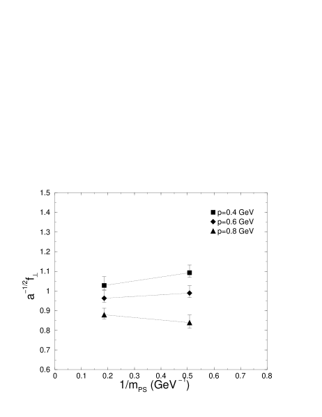
FIG. 8.: The heavy quark mass dependence at several momenta, at $\beta=5.9$ for the temporal matrix element. The light quarks are strange quarks. The dotted lines are to guide the eye.

There is a significant difference. The quarkonium spectrum tunes the (bare) heavy quark mass within a precision of 1–2% [14], which clearly would have no significant effect on the form factors. But because of lattice artifacts in the quarkonium binding energy [35] and because of quenching, the heavy-light spectrum yields a different adjustment of bare quark masses. The shift is to lower $1/m_{\text{PS}}$ in Fig. 8. From Eq. (9) one sees that $f_{\perp}$ dominates in $f_{+}$ for $B$ decay. Thus, $f_{+}$ is smaller with the heavy-light adjustment of the bottom quark mass, and $T_{B}$ is 6 percent smaller. On the other hand, $f_{\perp}$ and $f_{\parallel}$ make a comparable contributions to $f_{+}$ for $D$ decay. It turns out that $f_{+}$ is larger with the heavy-light adjustment of the charmed quark mass, and $T_{D}$ is 2 percent larger. The ratio $T_{B}/T_{D}$ is 8 percent smaller.

D Matching

As explained in Sec. II, our treatment of the heavy quark matches lattice gauge theory with Wilson fermions to HQET. This requires calculations of the short-distance coefficients: $1/m_{2}$ and $1/m_{\cal B}$ in the effective action; $\sqrt{Z_{V^{uu}}Z_{V^{bb}}}$ in the definition of the current; and $\rho_{V_{\parallel}}$, $\rho_{V_{\perp}}$, and $1/m_{3}$ in the description of the currents. As discussed in the previous subsection, $m_{2}$ is adjusted non-perturbatively, by tuning the quarkonium spectrum to agree with experiment. The normalization factors $Z_{V^{uu}}$ and $Z_{V^{bb}}$ are also computed non-perturbatively, by requiring that flavor-conserving matrix elements $\pi\to\pi$ and $B\to B$, computed by analogy with Eq. (27), give unit charge. The uncertainty from it is purely statistical and much smaller than all other statistical uncertainties.

The significant systematic effects in the matching procedure come from computing $\rho_{V_{\parallel}}$ and $\rho_{V_{\perp}}$, and from the mismatch between Eqs. (16) and Eqs. (17) at the level of dimension-four and higher currents. In the present work we do this part of the matching with perturbative QCD, leading to errors of order $\alpha_{s}^{2}$, $\alpha_{s}/m_{Q}$, $1/m_{Q}^{2}$, respectively. Let us now consider these effects in turn.

Because they are short-distance quantities, the matching factors $\rho_{V_{\parallel}}$ and $\rho_{V_{\perp}}$ should be calculable in perturbation theory. (Note that all effects that make lattice perturbation theory less reliable than continuum perturbation theory are absorbed into $\sqrt{Z_{V^{uu}}Z_{V^{bb}}}$.) We have calculated them to one loop, so we write

$$\rho_{V}=1+\alpha_{s}(q^{*})4\pi\rho_{V}^{[1]}$$ (37)

for $\rho_{V_{\parallel}}$ and $\rho_{V_{\perp}}$. We use the Brodsky-Lepage-Mackenzie (BLM) procedure to choose the expansion parameter $\alpha_{s}(q^{*})$ [36, 27]. In the scheme in which the Fourier transform of the heavy-quark potential reads $V(k)=-C_{F}4\pi\alpha_{s}(k)/k^{2}$, the BLM scale $q^{*}$ is given through

$$\log(q^{*}a)=\frac{{}^{*}\rho_{V}^{[1]}}{2\rho_{V}^{[1]}}$$ (38)

where ${}^{*}\rho_{V}^{[1]}$ is obtained from $\rho_{V}^{[1]}$ by replacing the gluon propagator $D(k)$ with $D(k)\log{k^{2}a^{2}}$. The details of these calculations are similar to those described in Ref. [37], and the results are listed in Table III [38].

TABLE III.: Perturbation theory for matching factors $\rho_{V_{\parallel}}$ and $\rho_{V_{\perp}}$. The one-loop terms $\rho_{V}^{[1]}$ and ${}^{*}\rho_{V}^{[1]}$ are in units of $10^{-5}$.

	$\beta=6.1$				$\beta=5.9$				$\beta=5.7$
	$\rho_{V}^{[1]}$	${}^{*}\rho_{V}^{[1]}$	$\alpha_{s}(q^{*})$	$\rho_{V}$	$\rho_{V}^{[1]}$	${}^{*}\rho_{V}^{[1]}$	$\alpha_{s}(q^{*})$	$\rho_{V}$	$\rho_{V}^{[1]}$	${}^{*}\rho_{V}^{[1]}$	$\alpha_{s}(q^{*})$	$\rho_{V}$
$b$
$f_{\parallel}$	536	980	0.159	1.011	817	1591	0.173	1.018	1065	2199	0.196	1.026
$f_{\perp}$	$-1987$	$-3312$	0.163	0.959	$-2096$	$-3534$	0.181	0.952	$-2146$	$-3621$	0.212	0.943
$c$
$f_{\parallel}$	$-59$	13	0.233	0.998	$-28$	40	0.402	0.999	$+63$	152	0.184	1.001
$f_{\perp}$	$-947$	$-1368$	0.169	0.980	$-1223$	$-1821$	0.188	0.971	$-1508$	$-2339$	0.218	0.959

The effects are small for $B$ decays and tiny for $D$ decays. This can be understood because the $\rho_{V}$s are ratios of very similar quantities, so there is good cancellation. It is therefore plausible that the two-loop contribution is numerically smaller by another factor of $\alpha_{s}\approx 0.2$, and thus completely negligible.

Next, we must estimate the uncertainty from the mismatch of the $1/m_{Q}$ term in the heavy-quark expansion. This contributes an error on either form factor $f$

$$\delta_{1/m_{Q}}f\sim\alpha_{s}b_{1/m_{Q}}(m_{Q}a)m_{Q}^{-1}\Lambda_{\text{QCD}}f$$ (39)

from $1/m_{3}$ and $1/m_{\cal B}$ contributions, and $b_{1/m_{Q}}$ gives the deviation of the short-distance coefficients for the lattice and continuum theories. (See Refs. [11, 12] for further details.) The factor $b(m_{Q}a)$ is at most of order unity; for our calculations of $D$-meson matrix elements it is of order $m_{c}a<1$. Taking $\alpha_{s}\approx 0.2$ and $\Lambda_{\text{QCD}}\approx 500$ MeV one finds that these errors, in either case, are at most a few percent on $f$ or the CKM matrix.

Finally, we must estimate the uncertainty from the mismatch of the $1/m_{Q}^{2}$ terms:

$$\delta_{1/m_{Q}^{2}}f\sim b_{1/m_{Q}^{2}}(m_{Q}a)m_{Q}^{-2}\Lambda_{\text{QCD}}^{2}f.$$ (40)

There are many contribution at order $1/m_{Q}^{2}$ in the heavy-quark expansion, most of which come from iteration of the $1/m_{Q}$ terms. Only genuine $1/m_{Q}^{2}$ terms in the effective action and currents can be as inaccurate as Eq. (40) suggests. Since $\Lambda_{\text{QCD}}/m_{Q}\approx\Lambda_{\text{QCD}}a\lesssim\alpha_{s}$ for our lattice data, the error $\delta_{1/m_{Q}^{2}}f$ is similar in magnitude to that of $\delta_{1/m_{Q}}f$.

The estimates in Table II derived from Eqs. (39) and (40) are very conservative. It is plausible that the denominator of heavy-quark expansion is $2m_{Q}$, and it is possible that the unknown coefficients are fractions instead of 1–2 as used above. Thus, the matching uncertainties may already be negligible.

The masses of the $b$ and $c$ quarks differ by about a factor of three. The short-distance coefficients are functions of $m_{Q}a$ [11, 12], so the matching uncertainties do not cancel completely in the ratio $T_{B}/T_{D}$. In particular, on our lattices the mismatch coefficients $b_{1/m_{Q}^{n}}$ are of order 1 for $b$ quarks, but $b_{1/m_{Q}}\sim m_{c}a$ and $b_{1/m_{Q}^{2}}\sim(m_{c}a)^{2},\,\alpha_{s}m_{c}a$ for $c$ quarks. Nevertheless, the effects often have the same sign, so we take the uncertainty in the ratio to be the same as in numerator or denominator.

E Lattice spacing dependence

For the artificial decays $B_{s},D_{s}\to\eta_{s}l\nu$ we have results at three lattice spacings, so we can examine how severely the form factors are affected. These decays are good for studying the $a$ dependence, because their form factors have small statistical errors. After chiral extrapolation, on the other hand, the larger statistical error bars would mask lattice spacing effects. Previous experience with decay constants [14] leads us to believe this will not change very much after chiral extrapolation. With the action used in this work the lattice spacing dependence is a combination of $O(\alpha_{s}a)$ and $O(a^{2})$ effects from the light quarks and gluons, and the $a$ dependence of the heavy-quark short-distance coefficients, discussed in the previous subsection. In particular, when the $\eta_{s}$ has non-zero recoil momentum $p$, the light-quark lattice effects are $O(\alpha_{s}pa)$ and $O(p^{2}a^{2})$.

The $a$ dependence of the form factors is shown in Fig. 9.

FIG. 9.: Lattice spacing dependence of $B_{s}\to\eta_{s}l\nu$ form factors (a) $f_{\parallel}$ and (b) $f_{\perp}$, for $p=0.5$ GeV (squares) and $0.7$ GeV (diamonds). The solid (open) symbols correspond to defining the lattice spacing with $\Delta m_{\text{1P-1S}}$ ($f_{\pi}$).

The variation with $a$ is several percent, which is comparable to the statistical uncertainty and also to the errors from the mismatch of the heavy quark. The observed $a$ dependence is therefore a combination of (uncorrelated) statistical fluctuations, lattice artifacts from the light degrees of freedom, and from the lattice artifacts [described in Eqs. (39) and (40)] of the heavy quark. They cannot be disentangled with the current set of calculations, so it does not make sense to extrapolate $a\to 0$.

Instead we choose the results from $\beta=5.9$, where we have the widest range of light quark masses, for our central value and use the other two lattices to estimate the uncertainty. Figure 10 shows the combination $p^{4}|f_{+}|^{2}/E$, which is proportional to $d\Gamma/dp$, at all three lattice spacings for $B_{s}\to\eta_{s}l\nu$ and $D_{s}\to\eta_{s}l\nu$.

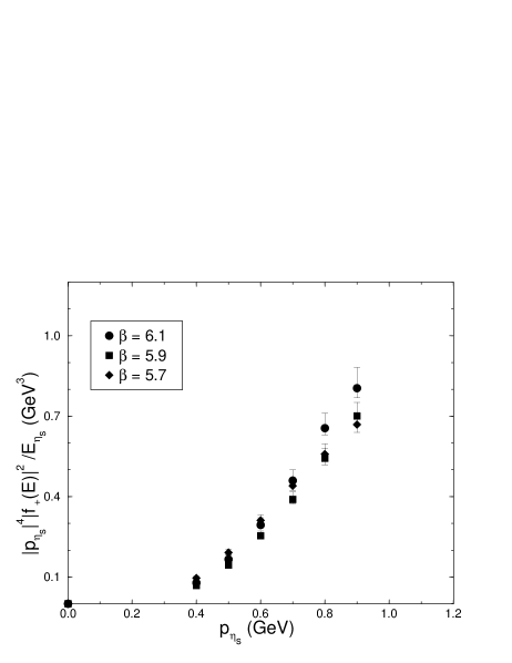
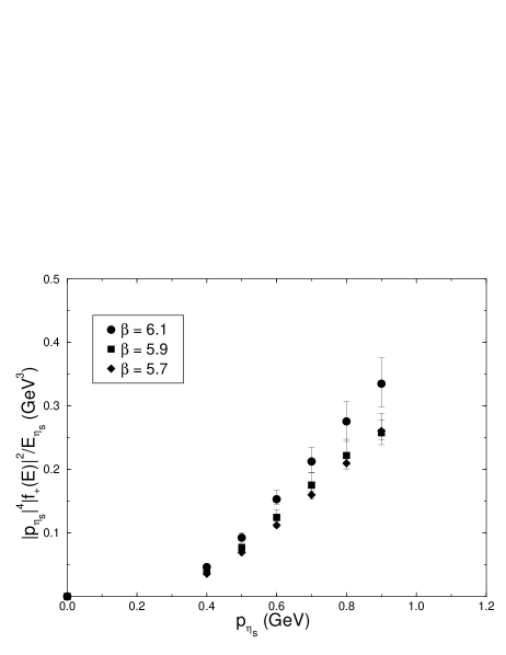
FIG. 10.: Comparison of $p^{4}|f_{+}|^{2}/E$ at three lattice spacings for (a) $B_{s}\to\eta_{s}l\nu$ and (b) $D_{s}\to\eta_{s}l\nu$.

As in Fig. 9 one sees that the dependence on $a$ is several percent, and increases with increasing $p$. By integrating over $p$ we find a variation of of $\hskip-5.0pt\raisebox{0.80002pt}{{$\;\begin{array}[]{@{}l@{}}\makebox[15.0pt][c]{$+$}\makebox[5.0pt][r]{16\hfill}\\[-2.40005pt] \makebox[15.0pt][c]{$-$}\makebox[5.0pt][r]{3\hfill}\end{array}$}}\%$ in $T_{B}$ and $\hskip-5.0pt\raisebox{0.80002pt}{{$\;\begin{array}[]{@{}l@{}}\makebox[15.0pt][c]{$+$}\makebox[5.0pt][r]{23\hfill}\\[-2.40005pt] \makebox[15.0pt][c]{$-$}\makebox[5.0pt][r]{6\hfill}\end{array}$}}\%$ in $T_{D}$.

F Definition of $a$ and quenching

Changes in the final results from changing the definition of $a$ can be thought of as a crude way to estimate effects of the quenched approximation. In lattice units we obtain $f_{\parallel}a^{1/2}$ and $f_{\perp}a^{-1/2}$, so converting to physical units introduces a mild explicit dependence on the value chosen for $a$. There is also an implicit dependence that enters through functional dependence on $E$ (or $p$). These two effects are illustrated in Fig. 9. The solid (open) points are obtained by defining $a$ so that the 1P-1S splitting of charmonium (pion decay constant) takes its physical value. The central values in the paper are computed with the 1P-1S definition. At $\beta=5.9$ we repeat the full analysis with the $f_{\pi}$ definition. We find that $T_{B}$ ($T_{D}$) increases by 11 percent (4 percent), and the ratio $T_{B}/T_{D}$ increases by 8 percent.

A more serious estimate of the effect of the quenched approximation is impossible without generating gauge fields with dynamical quark loops. This would require more computer resources than we have at our disposal, and no other group has yet studied these semileptonic decays with dynamical quarks. There are results with two light, dynamical flavors for the leptonic decay constants $f_{B}$ and $f_{D}$, using either lattice NRQCD [39] or our method [16, 40] for the heavy quark. In that case one finds an increase of between 10–11 percent over the quenched result.

The exercise of changing the definition of $a$ easily could underestimate the effects of quenching. At the same time, we do not expect form factors to be more sensitive than $f_{B}$. Thus, a provisional estimate of a uncertainty in $T_{B,D}$ of 10–20% seems reasonable.

VI Results

The main results of this paper, given in Eqs. (6) and (7), are the quantities $T_{B}(0.4~{}\text{GeV},1.0~{}\text{GeV})$ and $T_{D}(0.4~{}\text{GeV},0.925~{}\text{GeV})$, which are proportional to the partially integrated rates. It may also be of interest to present the results in other ways. In this section we give results for the ratio $T_{B}/T_{D}$, as well as results for $T_{B}$, $T_{D}$, and $T_{B}/T_{D}$ with a lower upper cut. We also give results for the form factors themselves.

Many uncertainties cancel in the ratio of $B$ and $D$ rates: the statistical error is correlated, and the systematic errors are similar in nature. Because of heavy-quark symmetry it is most sensible to form a ratio with the same cuts for both. We find

$$\frac{T_{B}(0.4~{}\text{GeV},0.9~{}\text{GeV})}{T_{D}(0.4~{}\text{GeV},0.9~{}\text{GeV})}=2.04^{+\,0.20}_{-\,0.09}{\;}^{+\,0.26}_{-\,0.08}\pm 0.10\pm 0.20\pm 0.29,$$ (41)

where the uncertainties are from statistics, chiral extrapolation, $a$ dependence, HQET matching, and other miscellaneous sources. A more detailed budget of the last uncertainty is given in Table II.

As mentioned above, raising the upper cut $p_{\text{max}}$ increases the uncertainty. Conversely, lowering $p_{\text{max}}$ decreases the uncertainty. Repeating the full analysis at $p_{\text{max}}=0.8~{}\text{GeV}$, we find

$$T_{B}(0.4~{}\text{GeV},0.8~{}\text{GeV}) = 0.294^{+\,0.063}_{-\,0.031}{\;}^{+\,0.041}_{-\,0.064}{\,}^{+\,0.041}_{-\,0.006}\pm 0.029\pm 0.038~{}\text{GeV}^{4},$$ (42)

$$T_{D}(0.4~{}\text{GeV},0.8~{}\text{GeV}) = 0.145^{+\,0.026}_{-\,0.013}{\;}\pm 0.016{\,}^{+\,0.024}_{-\,0.012}\pm 0.014\pm 0.017~{}\text{GeV}^{4}.$$ (43)

and the ratio

$$\frac{T_{B}(0.4~{}\text{GeV},0.8~{}\text{GeV})}{T_{D}(0.4~{}\text{GeV},0.8~{}\text{GeV})}=2.03^{+\,0.19}_{-\,0.10}{\;}^{+\,0.25}_{-\,0.16}\pm 0.10\pm 0.20\pm 0.24.$$ (44)

Table IV shows a budget of systematic errors, similar to Table II.

TABLE IV.: Budget of statistical and systematic uncertainties in this work for the quantities $T_{B}(0.4~{}\text{GeV},0.8~{}\text{GeV})$, $T_{D}(0.4~{}\text{GeV},0.8~{}\text{GeV})$, and $T_{B}(0.4~{}\text{GeV},0.8~{}\text{GeV})/T_{D}(0.4~{}\text{GeV},0.8~{}\text{GeV})$. All entries in percent.

uncertainty	$~{}T_{B}$	$|V_{ub}|$	$~{}T_{D}$	$|V_{cd}|$	$T_{B}/T_{D}$	$|V_{ub}/V_{cd}|$
statistical	$\;\begin{array}[]{@{}l@{}}\makebox[15.0pt][c]{$+$}\makebox[5.0pt][r]{21\hfill}\\[-2.40005pt] \makebox[15.0pt][c]{$-$}\makebox[5.0pt][r]{10\hfill}\end{array}$	$\;\begin{array}[]{@{}l@{}}\makebox[15.0pt][c]{$+$}\makebox[5.0pt][r]{11\hfill}\\[-2.40005pt] \makebox[15.0pt][c]{$-$}\makebox[5.0pt][r]{5\hfill}\end{array}$	$\;\begin{array}[]{@{}l@{}}\makebox[15.0pt][c]{$+$}\makebox[5.0pt][r]{18\hfill}\\[-2.40005pt] \makebox[15.0pt][c]{$-$}\makebox[5.0pt][r]{9\hfill}\end{array}$	$\;\begin{array}[]{@{}l@{}}\makebox[15.0pt][c]{$+$}\makebox[5.0pt][r]{9\hfill}\\[-2.40005pt] \makebox[15.0pt][c]{$-$}\makebox[5.0pt][r]{5\hfill}\end{array}$	$\;\begin{array}[]{@{}l@{}}\makebox[15.0pt][c]{$+$}\makebox[5.0pt][r]{10\hfill}\\[-2.40005pt] \makebox[15.0pt][c]{$-$}\makebox[5.0pt][r]{5\hfill}\end{array}$	$\;\begin{array}[]{@{}l@{}}\makebox[15.0pt][c]{$+$}\makebox[5.0pt][r]{5\hfill}\\[-2.40005pt] \makebox[15.0pt][c]{$-$}\makebox[5.0pt][r]{3\hfill}\end{array}$
excited states	4	2	4	2	4	2
$\textstyle p$ extrapolation	8	4	10	5	6	3
$m_{q}$ extrapolation	$\;\begin{array}[]{@{}l@{}}\makebox[15.0pt][c]{$+$}\makebox[5.0pt][r]{14\hfill}\\[-2.40005pt] \makebox[15.0pt][c]{$-$}\makebox[5.0pt][r]{22\hfill}\end{array}$	$\;\begin{array}[]{@{}l@{}}\makebox[15.0pt][c]{$+$}\makebox[5.0pt][r]{7\hfill}\\[-2.40005pt] \makebox[15.0pt][c]{$-$}\makebox[5.0pt][r]{11\hfill}\end{array}$	$\;\begin{array}[]{@{}l@{}}\makebox[15.0pt][c]{$+$}\makebox[5.0pt][r]{11\hfill}\\[-2.40005pt] \makebox[15.0pt][c]{$-$}\makebox[5.0pt][r]{11\hfill}\end{array}$	$\;\begin{array}[]{@{}l@{}}\makebox[15.0pt][c]{$+$}\makebox[2.5pt][r]{6\hfill}\\[-1.19995pt] \makebox[15.0pt][c]{$-$}\makebox[2.5pt][r]{6\hfill}\end{array}$	$\;\begin{array}[]{@{}l@{}}\makebox[15.0pt][c]{$+$}\makebox[5.0pt][r]{13\hfill}\\[-2.40005pt] \makebox[15.0pt][c]{$-$}\makebox[5.0pt][r]{8\hfill}\end{array}$	$\;\begin{array}[]{@{}l@{}}\makebox[15.0pt][c]{$+$}\makebox[2.5pt][r]{7\hfill}\\[-1.19995pt] \makebox[15.0pt][c]{$-$}\makebox[2.5pt][r]{4\hfill}\end{array}$
adjusting $m_{Q}$	3	1	4	2	6	3
HQET matching	10	5	10	5	10	5
$a$ dependence	$\;\begin{array}[]{@{}l@{}}\makebox[15.0pt][c]{$+$}\makebox[5.0pt][r]{14\hfill}\\[-2.40005pt] \makebox[15.0pt][c]{$-$}\makebox[5.0pt][r]{2\hfill}\end{array}$	$\;\begin{array}[]{@{}l@{}}\makebox[15.0pt][c]{$+$}\makebox[2.5pt][r]{7\hfill}\\[-1.19995pt] \makebox[15.0pt][c]{$-$}\makebox[2.5pt][r]{1\hfill}\end{array}$	$\;\begin{array}[]{@{}l@{}}\makebox[15.0pt][c]{$+$}\makebox[5.0pt][r]{17\hfill}\\[-2.40005pt] \makebox[15.0pt][c]{$-$}\makebox[5.0pt][r]{8\hfill}\end{array}$	$\;\begin{array}[]{@{}l@{}}\makebox[15.0pt][c]{$+$}\makebox[2.5pt][r]{9\hfill}\\[-1.19995pt] \makebox[15.0pt][c]{$-$}\makebox[2.5pt][r]{4\hfill}\end{array}$	5	3
definition of $a$	9	5	3	2	8	4
total systematic	$\;\begin{array}[]{@{}l@{}}\makebox[15.0pt][c]{$+$}\makebox[5.0pt][r]{26\hfill}\\[-2.40005pt] \makebox[15.0pt][c]{$-$}\makebox[5.0pt][r]{28\hfill}\end{array}$	$\;\begin{array}[]{@{}l@{}}\makebox[15.0pt][c]{$+$}\makebox[5.0pt][r]{13\hfill}\\[-2.40005pt] \makebox[15.0pt][c]{$-$}\makebox[5.0pt][r]{14\hfill}\end{array}$	$\;\begin{array}[]{@{}l@{}}\makebox[15.0pt][c]{$+$}\makebox[5.0pt][r]{26\hfill}\\[-2.40005pt] \makebox[15.0pt][c]{$-$}\makebox[5.0pt][r]{21\hfill}\end{array}$	$\;\begin{array}[]{@{}l@{}}\makebox[15.0pt][c]{$+$}\makebox[5.0pt][r]{13\hfill}\\[-2.40005pt] \makebox[15.0pt][c]{$-$}\makebox[5.0pt][r]{10\hfill}\end{array}$	$\;\begin{array}[]{@{}l@{}}\makebox[15.0pt][c]{$+$}\makebox[5.0pt][r]{21\hfill}\\[-2.40005pt] \makebox[15.0pt][c]{$-$}\makebox[5.0pt][r]{19\hfill}\end{array}$	$\;\begin{array}[]{@{}l@{}}\makebox[15.0pt][c]{$+$}\makebox[5.0pt][r]{11\hfill}\\[-2.40005pt] \makebox[15.0pt][c]{$-$}\makebox[5.0pt][r]{9\hfill}\end{array}$
total (stat $\oplus$ syst)	$\;\begin{array}[]{@{}l@{}}\makebox[15.0pt][c]{$+$}\makebox[5.0pt][r]{33\hfill}\\[-2.40005pt] \makebox[15.0pt][c]{$-$}\makebox[5.0pt][r]{29\hfill}\end{array}$	$\;\begin{array}[]{@{}l@{}}\makebox[15.0pt][c]{$+$}\makebox[5.0pt][r]{17\hfill}\\[-2.40005pt] \makebox[15.0pt][c]{$-$}\makebox[5.0pt][r]{15\hfill}\end{array}$	$\;\begin{array}[]{@{}l@{}}\makebox[15.0pt][c]{$+$}\makebox[5.0pt][r]{31\hfill}\\[-2.40005pt] \makebox[15.0pt][c]{$-$}\makebox[5.0pt][r]{23\hfill}\end{array}$	$\;\begin{array}[]{@{}l@{}}\makebox[15.0pt][c]{$+$}\makebox[5.0pt][r]{16\hfill}\\[-2.40005pt] \makebox[15.0pt][c]{$-$}\makebox[5.0pt][r]{11\hfill}\end{array}$	$\;\begin{array}[]{@{}l@{}}\makebox[15.0pt][c]{$+$}\makebox[5.0pt][r]{23\hfill}\\[-2.40005pt] \makebox[15.0pt][c]{$-$}\makebox[5.0pt][r]{20\hfill}\end{array}$	$\;\begin{array}[]{@{}l@{}}\makebox[15.0pt][c]{$+$}\makebox[5.0pt][r]{12\hfill}\\[-2.40005pt] \makebox[15.0pt][c]{$-$}\makebox[5.0pt][r]{9\hfill}\end{array}$

As one can see from comparing the last two lines in Tables II and IV, the total uncertainty is several percent lower with $p_{\text{max}}=0.8~{}\text{GeV}$.

Finally, we give our results for the form factors. Table V gives the results for form factors in the decay $B\to\pi l\nu$.

TABLE V.: Form factors with statistical and total systematic errors for the decay $B\to\pi l\nu$.

$p$	$E$	$q^{2}$	$f_{\parallel}$	$f_{\perp}$	$f_{+}$	$f_{0}$	$p^{4}|f_{+}|^{2}/E$
GeV	GeV	GeV2	GeV1/2	GeV-1/2			GeV3
0.0	0.140	26.41	1.93$\;\begin{array}[]{@{}l@{}}\makebox[15.0pt][c]{$+$}\makebox[5.0pt][r]{29\hfill}\\[-2.40005pt] \makebox[15.0pt][c]{$-$}\makebox[5.0pt][r]{3\hfill}\end{array}$$\;\begin{array}[]{@{}l@{}}\makebox[15.0pt][c]{$+$}\makebox[5.0pt][r]{28\hfill}\\[-2.40005pt] \makebox[15.0pt][c]{$-$}\makebox[5.0pt][r]{28\hfill}\end{array}$			1.17$\;\begin{array}[]{@{}l@{}}\makebox[15.0pt][c]{$+$}\makebox[5.0pt][r]{18\hfill}\\[-2.40005pt] \makebox[15.0pt][c]{$-$}\makebox[5.0pt][r]{6\hfill}\end{array}$$\;\begin{array}[]{@{}l@{}}\makebox[15.0pt][c]{$+$}\makebox[5.0pt][r]{18\hfill}\\[-2.40005pt] \makebox[15.0pt][c]{$-$}\makebox[5.0pt][r]{18\hfill}\end{array}$	0.0
0.1	0.172	26.07	1.88$\;\begin{array}[]{@{}l@{}}\makebox[15.0pt][c]{$+$}\makebox[5.0pt][r]{28\hfill}\\[-2.40005pt] \makebox[15.0pt][c]{$-$}\makebox[5.0pt][r]{3\hfill}\end{array}$$\;\begin{array}[]{@{}l@{}}\makebox[15.0pt][c]{$+$}\makebox[5.0pt][r]{28\hfill}\\[-2.40005pt] \makebox[15.0pt][c]{$-$}\makebox[5.0pt][r]{28\hfill}\end{array}$
0.2	0.244	25.31	1.85$\;\begin{array}[]{@{}l@{}}\makebox[15.0pt][c]{$+$}\makebox[5.0pt][r]{27\hfill}\\[-2.40005pt] \makebox[15.0pt][c]{$-$}\makebox[5.0pt][r]{3\hfill}\end{array}$$\;\begin{array}[]{@{}l@{}}\makebox[15.0pt][c]{$+$}\makebox[5.0pt][r]{28\hfill}\\[-2.40005pt] \makebox[15.0pt][c]{$-$}\makebox[5.0pt][r]{28\hfill}\end{array}$
0.3	0.331	24.39	1.80$\;\begin{array}[]{@{}l@{}}\makebox[15.0pt][c]{$+$}\makebox[5.0pt][r]{25\hfill}\\[-2.40005pt] \makebox[15.0pt][c]{$-$}\makebox[5.0pt][r]{4\hfill}\end{array}$$\;\begin{array}[]{@{}l@{}}\makebox[15.0pt][c]{$+$}\makebox[5.0pt][r]{27\hfill}\\[-2.40005pt] \makebox[15.0pt][c]{$-$}\makebox[5.0pt][r]{27\hfill}\end{array}$
0.4	0.424	23.41	1.73$\;\begin{array}[]{@{}l@{}}\makebox[15.0pt][c]{$+$}\makebox[5.0pt][r]{23\hfill}\\[-2.40005pt] \makebox[15.0pt][c]{$-$}\makebox[5.0pt][r]{4\hfill}\end{array}$$\;\begin{array}[]{@{}l@{}}\makebox[15.0pt][c]{$+$}\makebox[5.0pt][r]{26\hfill}\\[-2.40005pt] \makebox[15.0pt][c]{$-$}\makebox[5.0pt][r]{26\hfill}\end{array}$	1.05$\;\begin{array}[]{@{}l@{}}\makebox[15.0pt][c]{$+$}\makebox[5.0pt][r]{16\hfill}\\[-2.40005pt] \makebox[15.0pt][c]{$-$}\makebox[5.0pt][r]{18\hfill}\end{array}$$\;\begin{array}[]{@{}l@{}}\makebox[15.0pt][c]{$+$}\makebox[5.0pt][r]{16\hfill}\\[-2.40005pt] \makebox[15.0pt][c]{$-$}\makebox[5.0pt][r]{16\hfill}\end{array}$	2.10$\;\begin{array}[]{@{}l@{}}\makebox[15.0pt][c]{$+$}\makebox[5.0pt][r]{29\hfill}\\[-2.40005pt] \makebox[15.0pt][c]{$-$}\makebox[5.0pt][r]{25\hfill}\end{array}$$\;\begin{array}[]{@{}l@{}}\makebox[15.0pt][c]{$+$}\makebox[5.0pt][r]{32\hfill}\\[-2.40005pt] \makebox[15.0pt][c]{$-$}\makebox[5.0pt][r]{32\hfill}\end{array}$	1.00$\;\begin{array}[]{@{}l@{}}\makebox[15.0pt][c]{$+$}\makebox[5.0pt][r]{13\hfill}\\[-2.40005pt] \makebox[15.0pt][c]{$-$}\makebox[5.0pt][r]{3\hfill}\end{array}$$\;\begin{array}[]{@{}l@{}}\makebox[15.0pt][c]{$+$}\makebox[5.0pt][r]{15\hfill}\\[-2.40005pt] \makebox[15.0pt][c]{$-$}\makebox[5.0pt][r]{15\hfill}\end{array}$	0.27$\;\begin{array}[]{@{}l@{}}\makebox[15.0pt][c]{$+$}\makebox[2.5pt][r]{8\hfill}\\[-1.19995pt] \makebox[15.0pt][c]{$-$}\makebox[2.5pt][r]{6\hfill}\end{array}$
0.5	0.519	22.41	1.65$\;\begin{array}[]{@{}l@{}}\makebox[15.0pt][c]{$+$}\makebox[5.0pt][r]{21\hfill}\\[-2.40005pt] \makebox[15.0pt][c]{$-$}\makebox[5.0pt][r]{6\hfill}\end{array}$$\;\begin{array}[]{@{}l@{}}\makebox[15.0pt][c]{$+$}\makebox[5.0pt][r]{25\hfill}\\[-2.40005pt] \makebox[15.0pt][c]{$-$}\makebox[5.0pt][r]{25\hfill}\end{array}$	0.99$\;\begin{array}[]{@{}l@{}}\makebox[15.0pt][c]{$+$}\makebox[5.0pt][r]{13\hfill}\\[-2.40005pt] \makebox[15.0pt][c]{$-$}\makebox[5.0pt][r]{14\hfill}\end{array}$$\;\begin{array}[]{@{}l@{}}\makebox[15.0pt][c]{$+$}\makebox[5.0pt][r]{15\hfill}\\[-2.40005pt] \makebox[15.0pt][c]{$-$}\makebox[5.0pt][r]{15\hfill}\end{array}$	1.96$\;\begin{array}[]{@{}l@{}}\makebox[15.0pt][c]{$+$}\makebox[5.0pt][r]{24\hfill}\\[-2.40005pt] \makebox[15.0pt][c]{$-$}\makebox[5.0pt][r]{20\hfill}\end{array}$$\;\begin{array}[]{@{}l@{}}\makebox[15.0pt][c]{$+$}\makebox[5.0pt][r]{29\hfill}\\[-2.40005pt] \makebox[15.0pt][c]{$-$}\makebox[5.0pt][r]{29\hfill}\end{array}$	0.95$\;\begin{array}[]{@{}l@{}}\makebox[15.0pt][c]{$+$}\makebox[5.0pt][r]{12\hfill}\\[-2.40005pt] \makebox[15.0pt][c]{$-$}\makebox[5.0pt][r]{3\hfill}\end{array}$$\;\begin{array}[]{@{}l@{}}\makebox[15.0pt][c]{$+$}\makebox[5.0pt][r]{14\hfill}\\[-2.40005pt] \makebox[15.0pt][c]{$-$}\makebox[5.0pt][r]{14\hfill}\end{array}$	0.46$\;\begin{array}[]{@{}l@{}}\makebox[15.0pt][c]{$+$}\makebox[5.0pt][r]{12\hfill}\\[-2.40005pt] \makebox[15.0pt][c]{$-$}\makebox[5.0pt][r]{9\hfill}\end{array}$
0.6	0.616	21.38	1.56$\;\begin{array}[]{@{}l@{}}\makebox[15.0pt][c]{$+$}\makebox[5.0pt][r]{20\hfill}\\[-2.40005pt] \makebox[15.0pt][c]{$-$}\makebox[5.0pt][r]{7\hfill}\end{array}$$\;\begin{array}[]{@{}l@{}}\makebox[15.0pt][c]{$+$}\makebox[5.0pt][r]{23\hfill}\\[-2.40005pt] \makebox[15.0pt][c]{$-$}\makebox[5.0pt][r]{23\hfill}\end{array}$	0.95$\;\begin{array}[]{@{}l@{}}\makebox[15.0pt][c]{$+$}\makebox[5.0pt][r]{10\hfill}\\[-2.40005pt] \makebox[15.0pt][c]{$-$}\makebox[5.0pt][r]{9\hfill}\end{array}$$\;\begin{array}[]{@{}l@{}}\makebox[15.0pt][c]{$+$}\makebox[5.0pt][r]{14\hfill}\\[-2.40005pt] \makebox[15.0pt][c]{$-$}\makebox[5.0pt][r]{14\hfill}\end{array}$	1.84$\;\begin{array}[]{@{}l@{}}\makebox[15.0pt][c]{$+$}\makebox[5.0pt][r]{20\hfill}\\[-2.40005pt] \makebox[15.0pt][c]{$-$}\makebox[5.0pt][r]{14\hfill}\end{array}$$\;\begin{array}[]{@{}l@{}}\makebox[15.0pt][c]{$+$}\makebox[5.0pt][r]{27\hfill}\\[-2.40005pt] \makebox[15.0pt][c]{$-$}\makebox[5.0pt][r]{27\hfill}\end{array}$	0.89$\;\begin{array}[]{@{}l@{}}\makebox[15.0pt][c]{$+$}\makebox[5.0pt][r]{10\hfill}\\[-2.40005pt] \makebox[15.0pt][c]{$-$}\makebox[5.0pt][r]{4\hfill}\end{array}$$\;\begin{array}[]{@{}l@{}}\makebox[15.0pt][c]{$+$}\makebox[5.0pt][r]{13\hfill}\\[-2.40005pt] \makebox[15.0pt][c]{$-$}\makebox[5.0pt][r]{13\hfill}\end{array}$	0.71$\;\begin{array}[]{@{}l@{}}\makebox[15.0pt][c]{$+$}\makebox[5.0pt][r]{16\hfill}\\[-2.40005pt] \makebox[15.0pt][c]{$-$}\makebox[5.0pt][r]{10\hfill}\end{array}$
0.7	0.714	20.35	1.45$\;\begin{array}[]{@{}l@{}}\makebox[15.0pt][c]{$+$}\makebox[5.0pt][r]{18\hfill}\\[-2.40005pt] \makebox[15.0pt][c]{$-$}\makebox[5.0pt][r]{7\hfill}\end{array}$$\;\begin{array}[]{@{}l@{}}\makebox[15.0pt][c]{$+$}\makebox[5.0pt][r]{22\hfill}\\[-2.40005pt] \makebox[15.0pt][c]{$-$}\makebox[5.0pt][r]{22\hfill}\end{array}$	0.91$\;\begin{array}[]{@{}l@{}}\makebox[15.0pt][c]{$+$}\makebox[2.5pt][r]{9\hfill}\\[-1.19995pt] \makebox[15.0pt][c]{$-$}\makebox[2.5pt][r]{5\hfill}\end{array}$$\;\begin{array}[]{@{}l@{}}\makebox[15.0pt][c]{$+$}\makebox[5.0pt][r]{14\hfill}\\[-2.40005pt] \makebox[15.0pt][c]{$-$}\makebox[5.0pt][r]{14\hfill}\end{array}$	1.72$\;\begin{array}[]{@{}l@{}}\makebox[15.0pt][c]{$+$}\makebox[5.0pt][r]{18\hfill}\\[-2.40005pt] \makebox[15.0pt][c]{$-$}\makebox[5.0pt][r]{8\hfill}\end{array}$$\;\begin{array}[]{@{}l@{}}\makebox[15.0pt][c]{$+$}\makebox[5.0pt][r]{26\hfill}\\[-2.40005pt] \makebox[15.0pt][c]{$-$}\makebox[5.0pt][r]{26\hfill}\end{array}$	0.83$\;\begin{array}[]{@{}l@{}}\makebox[15.0pt][c]{$+$}\makebox[5.0pt][r]{10\hfill}\\[-2.40005pt] \makebox[15.0pt][c]{$-$}\makebox[5.0pt][r]{4\hfill}\end{array}$$\;\begin{array}[]{@{}l@{}}\makebox[15.0pt][c]{$+$}\makebox[5.0pt][r]{12\hfill}\\[-2.40005pt] \makebox[15.0pt][c]{$-$}\makebox[5.0pt][r]{12\hfill}\end{array}$	1.00$\;\begin{array}[]{@{}l@{}}\makebox[15.0pt][c]{$+$}\makebox[5.0pt][r]{22\hfill}\\[-2.40005pt] \makebox[15.0pt][c]{$-$}\makebox[5.0pt][r]{9\hfill}\end{array}$
0.8	0.812	19.31	1.34$\;\begin{array}[]{@{}l@{}}\makebox[15.0pt][c]{$+$}\makebox[5.0pt][r]{17\hfill}\\[-2.40005pt] \makebox[15.0pt][c]{$-$}\makebox[5.0pt][r]{8\hfill}\end{array}$$\;\begin{array}[]{@{}l@{}}\makebox[15.0pt][c]{$+$}\makebox[5.0pt][r]{20\hfill}\\[-2.40005pt] \makebox[15.0pt][c]{$-$}\makebox[5.0pt][r]{20\hfill}\end{array}$	0.86$\;\begin{array}[]{@{}l@{}}\makebox[15.0pt][c]{$+$}\makebox[5.0pt][r]{12\hfill}\\[-2.40005pt] \makebox[15.0pt][c]{$-$}\makebox[5.0pt][r]{4\hfill}\end{array}$$\;\begin{array}[]{@{}l@{}}\makebox[15.0pt][c]{$+$}\makebox[5.0pt][r]{13\hfill}\\[-2.40005pt] \makebox[15.0pt][c]{$-$}\makebox[5.0pt][r]{13\hfill}\end{array}$	1.59$\;\begin{array}[]{@{}l@{}}\makebox[15.0pt][c]{$+$}\makebox[5.0pt][r]{21\hfill}\\[-2.40005pt] \makebox[15.0pt][c]{$-$}\makebox[5.0pt][r]{7\hfill}\end{array}$$\;\begin{array}[]{@{}l@{}}\makebox[15.0pt][c]{$+$}\makebox[5.0pt][r]{24\hfill}\\[-2.40005pt] \makebox[15.0pt][c]{$-$}\makebox[5.0pt][r]{24\hfill}\end{array}$	0.76$\;\begin{array}[]{@{}l@{}}\makebox[15.0pt][c]{$+$}\makebox[5.0pt][r]{10\hfill}\\[-2.40005pt] \makebox[15.0pt][c]{$-$}\makebox[5.0pt][r]{4\hfill}\end{array}$$\;\begin{array}[]{@{}l@{}}\makebox[15.0pt][c]{$+$}\makebox[5.0pt][r]{11\hfill}\\[-2.40005pt] \makebox[15.0pt][c]{$-$}\makebox[5.0pt][r]{11\hfill}\end{array}$	1.27$\;\begin{array}[]{@{}l@{}}\makebox[15.0pt][c]{$+$}\makebox[5.0pt][r]{36\hfill}\\[-2.40005pt] \makebox[15.0pt][c]{$-$}\makebox[5.0pt][r]{11\hfill}\end{array}$
0.9	0.911	18.27	1.23$\;\begin{array}[]{@{}l@{}}\makebox[15.0pt][c]{$+$}\makebox[5.0pt][r]{17\hfill}\\[-2.40005pt] \makebox[15.0pt][c]{$-$}\makebox[5.0pt][r]{7\hfill}\end{array}$$\;\begin{array}[]{@{}l@{}}\makebox[15.0pt][c]{$+$}\makebox[5.0pt][r]{18\hfill}\\[-2.40005pt] \makebox[15.0pt][c]{$-$}\makebox[5.0pt][r]{18\hfill}\end{array}$	0.73$\;\begin{array}[]{@{}l@{}}\makebox[15.0pt][c]{$+$}\makebox[5.0pt][r]{15\hfill}\\[-2.40005pt] \makebox[15.0pt][c]{$-$}\makebox[5.0pt][r]{6\hfill}\end{array}$$\;\begin{array}[]{@{}l@{}}\makebox[15.0pt][c]{$+$}\makebox[5.0pt][r]{11\hfill}\\[-2.40005pt] \makebox[15.0pt][c]{$-$}\makebox[5.0pt][r]{11\hfill}\end{array}$	1.36$\;\begin{array}[]{@{}l@{}}\makebox[15.0pt][c]{$+$}\makebox[5.0pt][r]{23\hfill}\\[-2.40005pt] \makebox[15.0pt][c]{$-$}\makebox[5.0pt][r]{9\hfill}\end{array}$$\;\begin{array}[]{@{}l@{}}\makebox[15.0pt][c]{$+$}\makebox[5.0pt][r]{20\hfill}\\[-2.40005pt] \makebox[15.0pt][c]{$-$}\makebox[5.0pt][r]{20\hfill}\end{array}$	0.70$\;\begin{array}[]{@{}l@{}}\makebox[15.0pt][c]{$+$}\makebox[2.5pt][r]{9\hfill}\\[-1.19995pt] \makebox[15.0pt][c]{$-$}\makebox[2.5pt][r]{4\hfill}\end{array}$$\;\begin{array}[]{@{}l@{}}\makebox[15.0pt][c]{$+$}\makebox[5.0pt][r]{11\hfill}\\[-2.40005pt] \makebox[15.0pt][c]{$-$}\makebox[5.0pt][r]{11\hfill}\end{array}$	1.34$\;\begin{array}[]{@{}l@{}}\makebox[15.0pt][c]{$+$}\makebox[5.0pt][r]{51\hfill}\\[-2.40005pt] \makebox[15.0pt][c]{$-$}\makebox[5.0pt][r]{17\hfill}\end{array}$
1.0	1.01	17.23	1.15$\;\begin{array}[]{@{}l@{}}\makebox[15.0pt][c]{$+$}\makebox[5.0pt][r]{16\hfill}\\[-2.40005pt] \makebox[15.0pt][c]{$-$}\makebox[5.0pt][r]{6\hfill}\end{array}$$\;\begin{array}[]{@{}l@{}}\makebox[15.0pt][c]{$+$}\makebox[5.0pt][r]{17\hfill}\\[-2.40005pt] \makebox[15.0pt][c]{$-$}\makebox[5.0pt][r]{17\hfill}\end{array}$	0.59$\;\begin{array}[]{@{}l@{}}\makebox[15.0pt][c]{$+$}\makebox[5.0pt][r]{15\hfill}\\[-2.40005pt] \makebox[15.0pt][c]{$-$}\makebox[5.0pt][r]{6\hfill}\end{array}$$\;\begin{array}[]{@{}l@{}}\makebox[15.0pt][c]{$+$}\makebox[2.5pt][r]{9\hfill}\\[-1.19995pt] \makebox[15.0pt][c]{$-$}\makebox[2.5pt][r]{9\hfill}\end{array}$	1.13$\;\begin{array}[]{@{}l@{}}\makebox[15.0pt][c]{$+$}\makebox[5.0pt][r]{24\hfill}\\[-2.40005pt] \makebox[15.0pt][c]{$-$}\makebox[5.0pt][r]{9\hfill}\end{array}$$\;\begin{array}[]{@{}l@{}}\makebox[15.0pt][c]{$+$}\makebox[5.0pt][r]{17\hfill}\\[-2.40005pt] \makebox[15.0pt][c]{$-$}\makebox[5.0pt][r]{17\hfill}\end{array}$	0.64$\;\begin{array}[]{@{}l@{}}\makebox[15.0pt][c]{$+$}\makebox[2.5pt][r]{9\hfill}\\[-1.19995pt] \makebox[15.0pt][c]{$-$}\makebox[2.5pt][r]{3\hfill}\end{array}$$\;\begin{array}[]{@{}l@{}}\makebox[15.0pt][c]{$+$}\makebox[5.0pt][r]{10\hfill}\\[-2.40005pt] \makebox[15.0pt][c]{$-$}\makebox[5.0pt][r]{10\hfill}\end{array}$	1.30$\;\begin{array}[]{@{}l@{}}\makebox[15.0pt][c]{$+$}\makebox[5.0pt][r]{60\hfill}\\[-2.40005pt] \makebox[15.0pt][c]{$-$}\makebox[5.0pt][r]{35\hfill}\end{array}$

Listed are $f_{\parallel}$ and $f_{\perp}$, which emerge directly from our lattice calculations, and $f_{+}$ and $f_{0}$, which appear in the expression for the differential rate. In every case the first error is statistical and the second adds the systematic uncertainties in quadrature. Table VI lists the same information for $D\to\pi l\nu$.

TABLE VI.: Form factors with statistical and total systematic errors for the decay $D\to\pi l\nu$.

$p$	$E$	$q^{2}$	$f_{\parallel}$	$f_{\perp}$	$f_{+}$	$f_{0}$	$p^{4}|f_{+}|^{2}/E$
GeV	GeV	GeV2	GeV1/2	GeV-1/2			GeV3
0.0	0.140	2.99	1.34$\;\begin{array}[]{@{}l@{}}\makebox[15.0pt][c]{$+$}\makebox[5.0pt][r]{19\hfill}\\[-2.40005pt] \makebox[15.0pt][c]{$-$}\makebox[5.0pt][r]{3\hfill}\end{array}$$\;\begin{array}[]{@{}l@{}}\makebox[15.0pt][c]{$+$}\makebox[5.0pt][r]{17\hfill}\\[-2.40005pt] \makebox[15.0pt][c]{$-$}\makebox[5.0pt][r]{15\hfill}\end{array}$			1.29$\;\begin{array}[]{@{}l@{}}\makebox[15.0pt][c]{$+$}\makebox[5.0pt][r]{20\hfill}\\[-2.40005pt] \makebox[15.0pt][c]{$-$}\makebox[5.0pt][r]{2\hfill}\end{array}$$\;\begin{array}[]{@{}l@{}}\makebox[15.0pt][c]{$+$}\makebox[5.0pt][r]{17\hfill}\\[-2.40005pt] \makebox[15.0pt][c]{$-$}\makebox[5.0pt][r]{14\hfill}\end{array}$	0.0
0.1	0.172	2.87	1.33$\;\begin{array}[]{@{}l@{}}\makebox[15.0pt][c]{$+$}\makebox[5.0pt][r]{19\hfill}\\[-2.40005pt] \makebox[15.0pt][c]{$-$}\makebox[5.0pt][r]{2\hfill}\end{array}$$\;\begin{array}[]{@{}l@{}}\makebox[15.0pt][c]{$+$}\makebox[5.0pt][r]{17\hfill}\\[-2.40005pt] \makebox[15.0pt][c]{$-$}\makebox[5.0pt][r]{15\hfill}\end{array}$
0.2	0.244	2.60	1.32$\;\begin{array}[]{@{}l@{}}\makebox[15.0pt][c]{$+$}\makebox[5.0pt][r]{18\hfill}\\[-2.40005pt] \makebox[15.0pt][c]{$-$}\makebox[5.0pt][r]{2\hfill}\end{array}$$\;\begin{array}[]{@{}l@{}}\makebox[15.0pt][c]{$+$}\makebox[5.0pt][r]{17\hfill}\\[-2.40005pt] \makebox[15.0pt][c]{$-$}\makebox[5.0pt][r]{14\hfill}\end{array}$
0.3	0.331	2.28	1.31$\;\begin{array}[]{@{}l@{}}\makebox[15.0pt][c]{$+$}\makebox[5.0pt][r]{17\hfill}\\[-2.40005pt] \makebox[15.0pt][c]{$-$}\makebox[5.0pt][r]{3\hfill}\end{array}$$\;\begin{array}[]{@{}l@{}}\makebox[15.0pt][c]{$+$}\makebox[5.0pt][r]{17\hfill}\\[-2.40005pt] \makebox[15.0pt][c]{$-$}\makebox[5.0pt][r]{14\hfill}\end{array}$
0.4	0.424	1.93	1.28$\;\begin{array}[]{@{}l@{}}\makebox[15.0pt][c]{$+$}\makebox[5.0pt][r]{16\hfill}\\[-2.40005pt] \makebox[15.0pt][c]{$-$}\makebox[5.0pt][r]{4\hfill}\end{array}$$\;\begin{array}[]{@{}l@{}}\makebox[15.0pt][c]{$+$}\makebox[5.0pt][r]{16\hfill}\\[-2.40005pt] \makebox[15.0pt][c]{$-$}\makebox[5.0pt][r]{14\hfill}\end{array}$	1.19$\;\begin{array}[]{@{}l@{}}\makebox[15.0pt][c]{$+$}\makebox[5.0pt][r]{16\hfill}\\[-2.40005pt] \makebox[15.0pt][c]{$-$}\makebox[5.0pt][r]{15\hfill}\end{array}$$\;\begin{array}[]{@{}l@{}}\makebox[15.0pt][c]{$+$}\makebox[5.0pt][r]{15\hfill}\\[-2.40005pt] \makebox[15.0pt][c]{$-$}\makebox[5.0pt][r]{13\hfill}\end{array}$	1.56$\;\begin{array}[]{@{}l@{}}\makebox[15.0pt][c]{$+$}\makebox[5.0pt][r]{17\hfill}\\[-2.40005pt] \makebox[15.0pt][c]{$-$}\makebox[5.0pt][r]{10\hfill}\end{array}$$\;\begin{array}[]{@{}l@{}}\makebox[15.0pt][c]{$+$}\makebox[5.0pt][r]{20\hfill}\\[-2.40005pt] \makebox[15.0pt][c]{$-$}\makebox[5.0pt][r]{17\hfill}\end{array}$	1.14$\;\begin{array}[]{@{}l@{}}\makebox[15.0pt][c]{$+$}\makebox[5.0pt][r]{13\hfill}\\[-2.40005pt] \makebox[15.0pt][c]{$-$}\makebox[5.0pt][r]{4\hfill}\end{array}$$\;\begin{array}[]{@{}l@{}}\makebox[15.0pt][c]{$+$}\makebox[5.0pt][r]{15\hfill}\\[-2.40005pt] \makebox[15.0pt][c]{$-$}\makebox[5.0pt][r]{12\hfill}\end{array}$	0.15$\;\begin{array}[]{@{}l@{}}\makebox[15.0pt][c]{$+$}\makebox[2.5pt][r]{3\hfill}\\[-1.19995pt] \makebox[15.0pt][c]{$-$}\makebox[2.5pt][r]{2\hfill}\end{array}$
0.5	0.519	1.57	1.21$\;\begin{array}[]{@{}l@{}}\makebox[15.0pt][c]{$+$}\makebox[5.0pt][r]{15\hfill}\\[-2.40005pt] \makebox[15.0pt][c]{$-$}\makebox[5.0pt][r]{5\hfill}\end{array}$$\;\begin{array}[]{@{}l@{}}\makebox[15.0pt][c]{$+$}\makebox[5.0pt][r]{16\hfill}\\[-2.40005pt] \makebox[15.0pt][c]{$-$}\makebox[5.0pt][r]{13\hfill}\end{array}$	1.17$\;\begin{array}[]{@{}l@{}}\makebox[15.0pt][c]{$+$}\makebox[5.0pt][r]{12\hfill}\\[-2.40005pt] \makebox[15.0pt][c]{$-$}\makebox[5.0pt][r]{12\hfill}\end{array}$$\;\begin{array}[]{@{}l@{}}\makebox[15.0pt][c]{$+$}\makebox[5.0pt][r]{15\hfill}\\[-2.40005pt] \makebox[15.0pt][c]{$-$}\makebox[5.0pt][r]{13\hfill}\end{array}$	1.45$\;\begin{array}[]{@{}l@{}}\makebox[15.0pt][c]{$+$}\makebox[5.0pt][r]{14\hfill}\\[-2.40005pt] \makebox[15.0pt][c]{$-$}\makebox[5.0pt][r]{8\hfill}\end{array}$$\;\begin{array}[]{@{}l@{}}\makebox[15.0pt][c]{$+$}\makebox[5.0pt][r]{19\hfill}\\[-2.40005pt] \makebox[15.0pt][c]{$-$}\makebox[5.0pt][r]{16\hfill}\end{array}$	1.08$\;\begin{array}[]{@{}l@{}}\makebox[15.0pt][c]{$+$}\makebox[5.0pt][r]{12\hfill}\\[-2.40005pt] \makebox[15.0pt][c]{$-$}\makebox[5.0pt][r]{4\hfill}\end{array}$$\;\begin{array}[]{@{}l@{}}\makebox[15.0pt][c]{$+$}\makebox[5.0pt][r]{14\hfill}\\[-2.40005pt] \makebox[15.0pt][c]{$-$}\makebox[5.0pt][r]{12\hfill}\end{array}$	0.25$\;\begin{array}[]{@{}l@{}}\makebox[15.0pt][c]{$+$}\makebox[2.5pt][r]{5\hfill}\\[-1.19995pt] \makebox[15.0pt][c]{$-$}\makebox[2.5pt][r]{3\hfill}\end{array}$
0.6	0.616	1.21	1.12$\;\begin{array}[]{@{}l@{}}\makebox[15.0pt][c]{$+$}\makebox[5.0pt][r]{14\hfill}\\[-2.40005pt] \makebox[15.0pt][c]{$-$}\makebox[5.0pt][r]{6\hfill}\end{array}$$\;\begin{array}[]{@{}l@{}}\makebox[15.0pt][c]{$+$}\makebox[5.0pt][r]{15\hfill}\\[-2.40005pt] \makebox[15.0pt][c]{$-$}\makebox[5.0pt][r]{12\hfill}\end{array}$	1.13$\;\begin{array}[]{@{}l@{}}\makebox[15.0pt][c]{$+$}\makebox[5.0pt][r]{10\hfill}\\[-2.40005pt] \makebox[15.0pt][c]{$-$}\makebox[5.0pt][r]{8\hfill}\end{array}$$\;\begin{array}[]{@{}l@{}}\makebox[15.0pt][c]{$+$}\makebox[5.0pt][r]{15\hfill}\\[-2.40005pt] \makebox[15.0pt][c]{$-$}\makebox[5.0pt][r]{12\hfill}\end{array}$	1.32$\;\begin{array}[]{@{}l@{}}\makebox[15.0pt][c]{$+$}\makebox[5.0pt][r]{12\hfill}\\[-2.40005pt] \makebox[15.0pt][c]{$-$}\makebox[5.0pt][r]{6\hfill}\end{array}$$\;\begin{array}[]{@{}l@{}}\makebox[15.0pt][c]{$+$}\makebox[5.0pt][r]{17\hfill}\\[-2.40005pt] \makebox[15.0pt][c]{$-$}\makebox[5.0pt][r]{14\hfill}\end{array}$	1.01$\;\begin{array}[]{@{}l@{}}\makebox[15.0pt][c]{$+$}\makebox[5.0pt][r]{11\hfill}\\[-2.40005pt] \makebox[15.0pt][c]{$-$}\makebox[5.0pt][r]{5\hfill}\end{array}$$\;\begin{array}[]{@{}l@{}}\makebox[15.0pt][c]{$+$}\makebox[5.0pt][r]{13\hfill}\\[-2.40005pt] \makebox[15.0pt][c]{$-$}\makebox[5.0pt][r]{11\hfill}\end{array}$	0.36$\;\begin{array}[]{@{}l@{}}\makebox[15.0pt][c]{$+$}\makebox[2.5pt][r]{7\hfill}\\[-1.19995pt] \makebox[15.0pt][c]{$-$}\makebox[2.5pt][r]{3\hfill}\end{array}$
0.7	0.714	0.85	1.04$\;\begin{array}[]{@{}l@{}}\makebox[15.0pt][c]{$+$}\makebox[5.0pt][r]{13\hfill}\\[-2.40005pt] \makebox[15.0pt][c]{$-$}\makebox[5.0pt][r]{6\hfill}\end{array}$$\;\begin{array}[]{@{}l@{}}\makebox[15.0pt][c]{$+$}\makebox[5.0pt][r]{14\hfill}\\[-2.40005pt] \makebox[15.0pt][c]{$-$}\makebox[5.0pt][r]{11\hfill}\end{array}$	1.08$\;\begin{array}[]{@{}l@{}}\makebox[15.0pt][c]{$+$}\makebox[2.5pt][r]{7\hfill}\\[-1.19995pt] \makebox[15.0pt][c]{$-$}\makebox[2.5pt][r]{6\hfill}\end{array}$$\;\begin{array}[]{@{}l@{}}\makebox[15.0pt][c]{$+$}\makebox[5.0pt][r]{14\hfill}\\[-2.40005pt] \makebox[15.0pt][c]{$-$}\makebox[5.0pt][r]{12\hfill}\end{array}$	1.18$\;\begin{array}[]{@{}l@{}}\makebox[15.0pt][c]{$+$}\makebox[5.0pt][r]{10\hfill}\\[-2.40005pt] \makebox[15.0pt][c]{$-$}\makebox[5.0pt][r]{6\hfill}\end{array}$$\;\begin{array}[]{@{}l@{}}\makebox[15.0pt][c]{$+$}\makebox[5.0pt][r]{15\hfill}\\[-2.40005pt] \makebox[15.0pt][c]{$-$}\makebox[5.0pt][r]{13\hfill}\end{array}$	0.96$\;\begin{array}[]{@{}l@{}}\makebox[15.0pt][c]{$+$}\makebox[2.5pt][r]{9\hfill}\\[-1.19995pt] \makebox[15.0pt][c]{$-$}\makebox[2.5pt][r]{5\hfill}\end{array}$$\;\begin{array}[]{@{}l@{}}\makebox[15.0pt][c]{$+$}\makebox[5.0pt][r]{12\hfill}\\[-2.40005pt] \makebox[15.0pt][c]{$-$}\makebox[5.0pt][r]{10\hfill}\end{array}$	0.47$\;\begin{array}[]{@{}l@{}}\makebox[15.0pt][c]{$+$}\makebox[2.5pt][r]{8\hfill}\\[-1.19995pt] \makebox[15.0pt][c]{$-$}\makebox[2.5pt][r]{4\hfill}\end{array}$
0.8	0.812	0.478	0.99$\;\begin{array}[]{@{}l@{}}\makebox[15.0pt][c]{$+$}\makebox[5.0pt][r]{11\hfill}\\[-2.40005pt] \makebox[15.0pt][c]{$-$}\makebox[5.0pt][r]{6\hfill}\end{array}$$\;\begin{array}[]{@{}l@{}}\makebox[15.0pt][c]{$+$}\makebox[5.0pt][r]{13\hfill}\\[-2.40005pt] \makebox[15.0pt][c]{$-$}\makebox[5.0pt][r]{11\hfill}\end{array}$	1.02$\;\begin{array}[]{@{}l@{}}\makebox[15.0pt][c]{$+$}\makebox[2.5pt][r]{8\hfill}\\[-1.19995pt] \makebox[15.0pt][c]{$-$}\makebox[2.5pt][r]{6\hfill}\end{array}$$\;\begin{array}[]{@{}l@{}}\makebox[15.0pt][c]{$+$}\makebox[5.0pt][r]{13\hfill}\\[-2.40005pt] \makebox[15.0pt][c]{$-$}\makebox[5.0pt][r]{11\hfill}\end{array}$	1.07$\;\begin{array}[]{@{}l@{}}\makebox[15.0pt][c]{$+$}\makebox[2.5pt][r]{9\hfill}\\[-1.19995pt] \makebox[15.0pt][c]{$-$}\makebox[2.5pt][r]{6\hfill}\end{array}$$\;\begin{array}[]{@{}l@{}}\makebox[15.0pt][c]{$+$}\makebox[5.0pt][r]{14\hfill}\\[-2.40005pt] \makebox[15.0pt][c]{$-$}\makebox[5.0pt][r]{11\hfill}\end{array}$	0.95$\;\begin{array}[]{@{}l@{}}\makebox[15.0pt][c]{$+$}\makebox[2.5pt][r]{9\hfill}\\[-1.19995pt] \makebox[15.0pt][c]{$-$}\makebox[2.5pt][r]{5\hfill}\end{array}$$\;\begin{array}[]{@{}l@{}}\makebox[15.0pt][c]{$+$}\makebox[5.0pt][r]{12\hfill}\\[-2.40005pt] \makebox[15.0pt][c]{$-$}\makebox[5.0pt][r]{10\hfill}\end{array}$	0.58$\;\begin{array}[]{@{}l@{}}\makebox[15.0pt][c]{$+$}\makebox[5.0pt][r]{11\hfill}\\[-2.40005pt] \makebox[15.0pt][c]{$-$}\makebox[5.0pt][r]{6\hfill}\end{array}$
0.9	0.911	0.109	0.95$\;\begin{array}[]{@{}l@{}}\makebox[15.0pt][c]{$+$}\makebox[5.0pt][r]{10\hfill}\\[-2.40005pt] \makebox[15.0pt][c]{$-$}\makebox[5.0pt][r]{5\hfill}\end{array}$$\;\begin{array}[]{@{}l@{}}\makebox[15.0pt][c]{$+$}\makebox[5.0pt][r]{12\hfill}\\[-2.40005pt] \makebox[15.0pt][c]{$-$}\makebox[5.0pt][r]{10\hfill}\end{array}$	0.98$\;\begin{array}[]{@{}l@{}}\makebox[15.0pt][c]{$+$}\makebox[2.5pt][r]{8\hfill}\\[-1.19995pt] \makebox[15.0pt][c]{$-$}\makebox[2.5pt][r]{7\hfill}\end{array}$$\;\begin{array}[]{@{}l@{}}\makebox[15.0pt][c]{$+$}\makebox[5.0pt][r]{13\hfill}\\[-2.40005pt] \makebox[15.0pt][c]{$-$}\makebox[5.0pt][r]{11\hfill}\end{array}$	0.98$\;\begin{array}[]{@{}l@{}}\makebox[15.0pt][c]{$+$}\makebox[2.5pt][r]{9\hfill}\\[-1.19995pt] \makebox[15.0pt][c]{$-$}\makebox[2.5pt][r]{6\hfill}\end{array}$$\;\begin{array}[]{@{}l@{}}\makebox[15.0pt][c]{$+$}\makebox[5.0pt][r]{13\hfill}\\[-2.40005pt] \makebox[15.0pt][c]{$-$}\makebox[5.0pt][r]{11\hfill}\end{array}$	0.94$\;\begin{array}[]{@{}l@{}}\makebox[15.0pt][c]{$+$}\makebox[2.5pt][r]{9\hfill}\\[-1.19995pt] \makebox[15.0pt][c]{$-$}\makebox[2.5pt][r]{5\hfill}\end{array}$$\;\begin{array}[]{@{}l@{}}\makebox[15.0pt][c]{$+$}\makebox[5.0pt][r]{12\hfill}\\[-2.40005pt] \makebox[15.0pt][c]{$-$}\makebox[5.0pt][r]{10\hfill}\end{array}$	0.69$\;\begin{array}[]{@{}l@{}}\makebox[15.0pt][c]{$+$}\makebox[5.0pt][r]{13\hfill}\\[-2.40005pt] \makebox[15.0pt][c]{$-$}\makebox[5.0pt][r]{8\hfill}\end{array}$
0.925	0.935	0	0.93$\;\begin{array}[]{@{}l@{}}\makebox[15.0pt][c]{$+$}\makebox[5.0pt][r]{13\hfill}\\[-2.40005pt] \makebox[15.0pt][c]{$-$}\makebox[5.0pt][r]{4\hfill}\end{array}$$\;\begin{array}[]{@{}l@{}}\makebox[15.0pt][c]{$+$}\makebox[5.0pt][r]{12\hfill}\\[-2.40005pt] \makebox[15.0pt][c]{$-$}\makebox[5.0pt][r]{10\hfill}\end{array}$	0.95$\;\begin{array}[]{@{}l@{}}\makebox[15.0pt][c]{$+$}\makebox[2.5pt][r]{9\hfill}\\[-1.19995pt] \makebox[15.0pt][c]{$-$}\makebox[2.5pt][r]{7\hfill}\end{array}$$\;\begin{array}[]{@{}l@{}}\makebox[15.0pt][c]{$+$}\makebox[5.0pt][r]{12\hfill}\\[-2.40005pt] \makebox[15.0pt][c]{$-$}\makebox[5.0pt][r]{10\hfill}\end{array}$	0.94$\;\begin{array}[]{@{}l@{}}\makebox[15.0pt][c]{$+$}\makebox[5.0pt][r]{10\hfill}\\[-2.40005pt] \makebox[15.0pt][c]{$-$}\makebox[5.0pt][r]{5\hfill}\end{array}$$\;\begin{array}[]{@{}l@{}}\makebox[15.0pt][c]{$+$}\makebox[5.0pt][r]{12\hfill}\\[-2.40005pt] \makebox[15.0pt][c]{$-$}\makebox[5.0pt][r]{10\hfill}\end{array}$	0.94$\;\begin{array}[]{@{}l@{}}\makebox[15.0pt][c]{$+$}\makebox[5.0pt][r]{10\hfill}\\[-2.40005pt] \makebox[15.0pt][c]{$-$}\makebox[5.0pt][r]{6\hfill}\end{array}$$\;\begin{array}[]{@{}l@{}}\makebox[15.0pt][c]{$+$}\makebox[5.0pt][r]{12\hfill}\\[-2.40005pt] \makebox[15.0pt][c]{$-$}\makebox[5.0pt][r]{10\hfill}\end{array}$	0.71$\;\begin{array}[]{@{}l@{}}\makebox[15.0pt][c]{$+$}\makebox[5.0pt][r]{19\hfill}\\[-2.40005pt] \makebox[15.0pt][c]{$-$}\makebox[5.0pt][r]{9\hfill}\end{array}$

Our final results for $f_{\parallel}$ and $f_{\perp}$ are obtained at $\beta=5.9$, after chiral extrapolation, with the systematic errors estimated as described in Sec. V. In particular, the estimate of lattice spacing effects uses results from all three lattice spacings. For $p<0.4$ GeV our extrapolation of $f_{\perp}$ in the pion momentum is no longer reliable, so we do not quote results for it.

The physical form factors $f_{+}(E)$ and $f_{0}(E)$ are obtained from Eqs. (9) and (10) using the tabulated results for $f_{\perp}(E)$ and $f_{\parallel}(E)$, physical meson masses, and energy $E=\sqrt{m_{\pi}^{2}+p^{2}}$, for each $p=|\mathchoice{{\hbox{\boldmath$\displaystyle p$}}}{{\hbox{\boldmath$\textstyle p$}}}{{\hbox{\boldmath$\scriptstyle p$}}}{{\hbox{\boldmath$\scriptscriptstyle p$}}}_{\pi}|$ in our set of pion three-momenta. They are shown in Fig. 11.

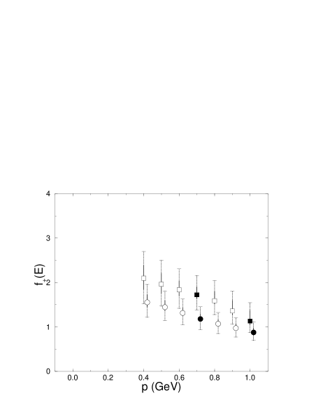
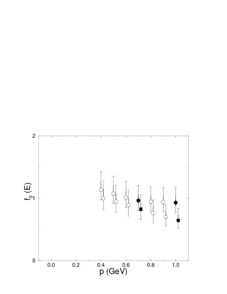
FIG. 11.: Momentum dependence of the form factors with all systematic uncertainties included. (a) $f_{+}$ and (b) $f_{0}$. Squares (circles) denote $B$ ($D$) decays. Solid symbols are independent of the momentum interpolation.

Tables V and VI also include the combination $p^{4}|f^{+}|^{2}/E$; for massless final-state leptons the differential rates are given by

$$\frac{d\Gamma_{B\to\pi}}{dp\hfil}=|V_{ub}|^{2}\,(2.9328~{}\text{ps}^{-1}\text{GeV}^{-4})\,\frac{p^{4}|f_{+}|^{2}}{E},$$ (45)

$$\frac{d\Gamma_{D\to\pi}}{dp\hfil}=|V_{cd}|^{2}\,(1.0358~{}\text{ps}^{-1}\text{GeV}^{-4})\,\frac{p^{4}|f_{+}|^{2}}{E}.$$ (46)

Other differential distributions can be obtained from the latter by changing variables with $dp/dE=E/p$ and $dp/dq^{2}=E/2m_{B}p$ or $E/2m_{D}p$. From Eqs. (45) and (46) one sees that the phase-space factor $p^{4}$ suppresses the rate in the low-momentum region where we cannot quote $f_{+}$.

VII Comparison with other results

In this section we compare our results to recent published [19, 20] and preliminary [21] work from lattice QCD. The comparison is apt, because three different methods for treating the heavy quark on the lattice have been employed. We use Wilson fermions with the SW action, normalized to have a consistent heavy-quark limit. References [19, 20] use Wilson fermions (with the SW action and light-quark normalization conditions) at $m_{Q}$ near and below the charmed quark mass, and extrapolate up to $m_{b}$. Reference [21] uses lattice NRQCD [41] (with the power-counting of HQET [42]) and, as we do, calculates the form factors directly at the bottom quark mass.

Figure 12 shows results from Refs. [19, 20] together with ours. (We do not include results from the JLQCD collaboration [21], because they are still preliminary. We anticipate that their systematic uncertainties will be similar to ours. At this stage their statistical uncertainties seem surprisingly large.) Within the quoted uncertainties there is broad agreement among the three calculations. There are, however, three noteworthy differences in the analysis of the form factors. These are the lattice spacings at which the calculations are done, the procedure for chiral extrapolation, and the treatment of the heavy quark.

Our results are based on lattice gauge fields at three lattice spacings, given in Table I.

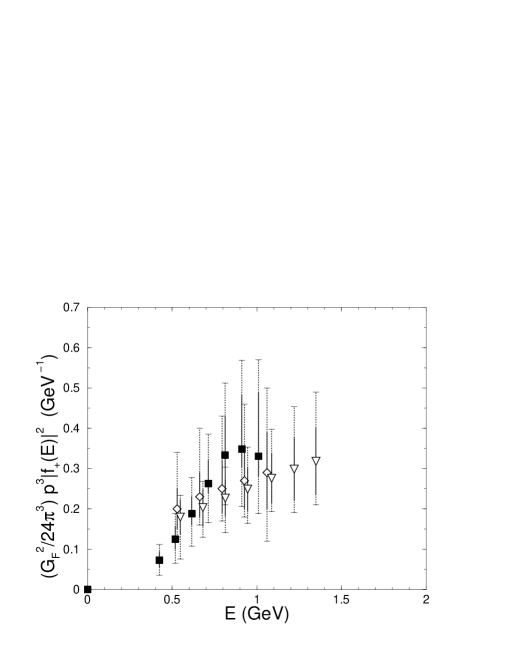
FIG. 12.: Comparison of the differential decay rate (at fixed lattice spacing) vs. $E$: open diamonds [19], open triangles [20], and solid squares (this work).

We find that the lattice-spacing dependence of the form factors is mild (with our treatment of the heavy quark), even on a relatively coarse lattice at $\beta=5.7$. The results of Refs. [19, 20] are both based on only one set of lattice gauge fields (at $\beta=6.2$), whose spacing is slightly finer than any of ours. We believe, therefore, that the lattice spacing effects of the gluons and light quarks are not a serious source of error, at the present overall level of accuracy, in any of the three works.

In our work, the largest uncertainty comes from the chiral extrapolation at fixed pion momentum $p$. As explained in Sec. V B, this uncertainty arises because the linear and quadratic fits give moderately different results. References [19, 20] do not have enough values of the light quark mass to be able to check whether a term quadratic in $m_{q}$ is needed to describe their data. Because those works extrapolate at fixed $q^{2}$, however, it is plausible that the curvature seen in Fig. 7 would go away, and that a linear chiral extrapolation would then be adequate.

The interpolation in pion momentum, or energy, is another difference. It leads to the apparent difference in the shape of the spectrum in Fig. 12. If we choose the pole form suggested (for small $E$) by Eqs. (11) and (12), the shape of the spectrum is less humped, though not as flat as the spectra from Refs. [19, 20]. In those works a pole Ansatz different from Eqs. (11) and (12) was used.

The most significant difference in the three calculations is the treatment of the heavy quark. Although the same action and similar currents are used, the bare quark mass and the normalization of the current are adjusted differently. The normalization conditions chosen in Refs. [19, 20] are designed for the $m_{Q}a\to 0$ limit, and at finite $m_{Q}a$ they leave systematic uncertainties of order $(m_{Q}a)^{2}$. To reduce these, Refs. [19, 20] calculate with the heavy-light meson mass near and below 2 GeV and extrapolate up to $m_{B}$. This procedure leads to their largest quoted uncertainty. The statistical error increases, as it must in any extrapolation. There are also systematic effects, which are estimated by trying linear and quadratic fits in $1/m_{Q}$. For at least two reasons, this test may underestimate the systematic uncertainty of the extrapolation. First, the compatibility of the fits shows only that the dependence on $1/m_{Q}$ is smooth in the employed range of the quark masses. It does not show that the heavy-quark expansion is reliable below 2 GeV. This problem is especially severe for Ref. [19], which has heavy-light meson masses as low as 1.2 GeV. Second, the lattice artifacts of order $(m_{Q}a)^{2}$ may well be amplified by the extrapolation. This problem would be especially severe for Ref. [20], which has $m_{Q}a$ as high as 0.7.

Our normalization conditions coincide with those above as $m_{Q}a\to 0$. At finite $m_{Q}a$, however, they are chosen to eliminate lattice artifacts that grow with $m_{Q}a$ [11]. This is made possible by using HQET to match the lattice action and current to continuum QCD [12], as reviewed in Sec. II. The advantage is that, as with lattice NRQCD [41, 21], the calculations can be done directly at $m_{Q}=m_{b}$, without an extrapolation in $1/m_{Q}$. Of course, we must assume that HQET is valid for the $b$ quark, but that is safer than assuming that it is valid for $m_{Q}\sim 1$–2 GeV.

A feature of our approach is that it leads to a somewhat complicated pattern of heavy-quark discretization errors. There is, however, a corresponding pattern of systematic uncertainties in the results of Refs. [19, 20]. In particular, there are corrections to the normalization of order $\alpha_{s}(m_{Q}a)^{2}$ and of order $(m_{Q}a)^{2}\Lambda_{\text{QCD}}/m_{Q}=m_{Q}a\Lambda_{\text{QCD}}a$ in the $1/m_{Q}$ term of the heavy-quark expansion. Estimates of the magnitude of these errors—before or after $1/m_{Q}$ extrapolation—are absent from Refs. [19, 20]. (The corresponding errors in our work, which we address quantitatively in Sec. V D, are of order $\alpha_{s}^{2}$ in the normalization and of order $\alpha_{s}\Lambda_{\text{QCD}}/m_{b}$ in the $1/m_{Q}$ term.)

The calculation of semileptonic form factors for $B\to\pi l\nu$, and related $D$ decays, has also been carried out with quark models and QCD sum rules. At present the uncertainties from lattice QCD are comparable to those based on light-cone sum rules [43, 44]. The latter have the advantage that they are most applicable for energetic pions, so (for $B$ decay) they overlap better with th distribution of events in an experiment. On the other hand, it seems difficult to reduce the uncertainties from sum rules down to the level of a few percent, which will be needed to match the precision of the $B$ factories. As discussed in the following section, however, all uncertainties of the form factors are reducible with lattice QCD.

VIII Conclusions

In this paper we have presented results for the form factors and differential decay rates for the semileptonic decays $B\to\pi l\nu$ and $D\to\pi l\nu$. The total uncertainties are 30–35 percent (for the rate) and, hence, would yield a theoretical uncertainty to the CKM matrix of 15–18 percent. We have attempted a complete analysis of the systematic uncertainties, at least within the quenched approximation. A rough estimate of the additional error from quenching is 10–20 percent (on the rate).

A more important, thought less specific, result of this paper is a demonstration that, within the quenched approximation, all uncertainties are controllable. Table VII gives a sketch of what is needed to reduce all sources of uncertainty.

TABLE VII.: Strategies for reducing statistical and systematic uncertainties of semileptonic form factors.

uncertainty	strategy
statistical	more lattice gauge fields; better $m_{q}$ extrapolation
excited states	longer time extent; better operators
$\textstyle p$ extrapolation	larger finite volume; better statistics
$m_{q}$ extrapolation	better statistics; more values of $m_{q}$; fixed-$E$ extrapolation
adjusting $m_{Q}$	unquench
HQET matching	match up to $\alpha_{s}\Lambda_{\text{QCD}}/m_{Q}$, $(\Lambda_{\text{QCD}}/m_{Q})^{2}$
$a$ dependence	more lattices
definition of $a$	unquench
quenching	unquench

In almost every case, the remedy is simply more computer time. That, in fact, is promising, since the computer used in this work is already ten years old. Given the experience of the CP-PACS [16, 39] and MILC [40] collaborations with heavy-light decay constants, it should be feasible to repeat our analysis on a modern supercomputer with unquenched gauge fields. In summary, there do not appear to be any technical roadblocks to reducing the uncertainties in lattice calculations to a few percent or better, over the course of the present round of experiments.

In the case of the uncertainty labeled “HQET matching” better calculations of the various short-distance coefficients introduced in Sec. II will be needed to be sure that the total uncertainty is only a few percent. This is not a computational problem but a theoretical one, which arises also in calculations with lattice NRQCD. The alternative would be to reduce the lattice spacing dramatically, so that $m_{Q}a$ and $\Lambda_{\text{QCD}}/m_{Q}$ can be simultaneously small. But, since computer requirements scale as $a^{-1}$ to a high power, that would seem to be a long way off. One would also have to sacrifice some other improvements, such as removing the quenched approximation.

For semileptonic decays of $B$ or$D$ to vector mesons such as $\rho$ and $\omega$ more study is needed. The vector mesons decay hadronically, and in the quenched approximation these decays are absent. Even in unquenched calculations, however, there are still issues that may need explicit analysis. In particular, if the calculations are done at largish light quark masses, the decay may be kinematically forbidden. Because there is not yet much experience with unquenched calculations, it is not yet clear whether one can smoothly extrapolate vector meson properties from this region to the physical meson masses. It is, thus, hard to anticipate how well lattice QCD will do here. This is unfortunate, because the experimental errors for semileptonic decays into vector mesons are expected to be somewhat smaller.

In any case, semileptonic decays of $B$ mesons ultimately will provide one of the most accurate constraints on the unitarity triangle, through a determination of $|V_{ub}|$. Indeed, if new physics lurks behind $B^{0}$-$\bar{B}^{0}$ mixing, it is essential to have constraints on the CKM matrix through charged-current interactions like $b\to c$ and $b\to u$.

- [1] D. E. Groom et al., Eur. Phys. J. C15, 1 (2000).
- [2] For a review and guide to the literature on inclusive decays, see Z. Ligeti, “ and from Decays: Recent Progress and Limitations,” in Kaon Physics, edited by J. L. Rosner and B. D. Winstein (U. of Chicago, Chicago, 2000) [hep-ph/9908432].
- [3] A. S. Kronfeld and J. N. Simone, Phys. Lett. B490, 228 (2000).
- [4] H. Albrecht et al. [ARGUS Collaboration], Phys. Lett. B255, 297 (1991); J. Bartelt et al. [CLEO Collaboration], Phys. Rev. Lett. 71, 4111 (1993).
- [5] A. F. Falk, Z. Ligeti and M. B. Wise, Phys. Lett. B406, 225 (1997).
- [6] C. W. Bauer, Z. Ligeti, and M. Luke, Phys. Lett. B479, 395 (2000).
- [7] P. L. Frabetti et al. [E687 Collaboration], Phys. Lett. B364, 127 (1995).
- [8] B. O’Reilly [FOCUS Collaboration], Nucl. Phys. B Proc. Suppl. 75B, 20 (1999).
- [9] J. P. Alexander et al. [CLEO Collaboration], Phys. Rev. Lett. 77, 5000 (1996).
- [10] B. H. Behrens et al. [CLEO Collaboration], Phys. Rev. D61, 052001 (2000).
- [11] A. X. El-Khadra, A. S. Kronfeld, and P. B. Mackenzie, Phys. Rev. D55, 3933 (1997).
- [12] A. S. Kronfeld, Phys. Rev. D62, 014505 (2000).
- [13] S. Aoki et al. [JLQCD Collaboration], Phys. Rev. Lett. 80, 5711 (1998).
- [14] A. X. El-Khadra et al., Phys. Rev. D58, 014506 (1998).
- [15] C. Bernard et al., Phys. Rev. Lett. 81, 4812 (1998).
- [16] A. Ali Khan et al. [CP-PACS Collaboration], Nucl. Phys. B Proc. Suppl. 83, 331 (2000); hep-lat/0010009.
- [17] S. Hashimoto et al., Phys. Rev. D61, 014502 (2000); J. N. Simone et al., Nucl. Phys. B Proc. Suppl. 83, 334 (2000).
- [18] K. C. Bowler et al. [UKQCD Collaboration], Phys. Rev. D51, 4905 (1995).
- [19] K. C. Bowler et al. [UKQCD Collaboration], Nucl. Phys. B Proc. Suppl. 83, 313 (2000); Phys. Lett. B486, 111 (2000).
- [20] A. Abada, D. Becirevic, P. Boucaud, J. P. Leroy, V. Lubicz and F. Mescia, hep-lat/0011065.
- [21] S. Aoki et al. [JLQCD Collaboration], Nucl. Phys. B Proc. Suppl. 83, 325 (2000); hep-lat/0011008.
- [22] J. N. Simone, Nucl. Phys. B Proc. Suppl. 47, 17 (1996).
- [23] S. Ryan et al., Nucl. Phys. B Proc. Suppl. 73, 390 (1999); 83, 328 (2000); S. M. Ryan, hep-ph/9905232.
- [24] J. N. Simone et al., Nucl. Phys. B Proc. Suppl. 73, 393 (1999).
- [25] G. Burdman, Z. Ligeti, M. Neubert, and Y. Nir, Phys. Rev. D49, 2331 (1994). The form factors introduced here are related to those in Eq. (8) by , .
- [26] B. Sheikholeslami and R. Wohlert, Nucl. Phys. B259, 572 (1985).
- [27] G. P. Lepage and P. B. Mackenzie, Phys. Rev. D48, 2250 (1993).
- [28] A. Duncan et al., Phys. Rev. D51, 5101 (1995).
- [29] B. J. Gough et al., Phys. Rev. Lett. 79, 1622 (1997).
- [30] A. X. El-Khadra, G. Hockney, A. S. Kronfeld, and P. B. Mackenzie, Phys. Rev. Lett. 69, 729 (1992).
- [31] A. Duncan, E. Eichten, and H. Thacker, Phys. Lett. B303, 109 (1993).
- [32] T. Onogi and J. N. Simone, Nucl. Phys. B Proc. Suppl. 42, 434 (1995).
- [33] W. Bardeen, A. Duncan, E. Eichten, G. Hockney, and H. Thacker, Phys. Rev. D57, 1633 (1998).
- [34] L. Lellouch, Nucl. Phys. B479, 353 (1996).
- [35] A. S. Kronfeld, Nucl. Phys. B Proc. Suppl. 53, 401 (1997); Nucl. Phys. B Proc. Suppl. 63, 311 (1998).
- [36] S. J. Brodsky, G. P. Lepage, and P. B. Mackenzie, Phys. Rev. D28, 228 (1983).
- [37] A. S. Kronfeld and S. Hashimoto, Nucl. Phys. B Proc. Suppl. 73, 387 (1999).
- [38] J. Harada, S. Hashimoto, K.-I. Ishikawa, A. S. Kronfeld, T. Onogi, and N. Yamada, in preparation.
- [39] A. Ali Khan et al. [CP-PACS Collaboration], Nucl. Phys. B Proc. Suppl. 83, 265 (2000).
- [40] C. Bernard et al. [MILC Collaboration], Nucl. Phys. B Proc. Suppl. 83, 289 (2000).
- [41] G. P. Lepage and B. A. Thacker, Nucl. Phys. B Proc. Suppl. 4, 199 (1987); B. A. Thacker and G. P. Lepage, Phys. Rev. D43, 196 (1991); G. P. Lepage, L. Magnea, C. Nakhleh, U. Magnea, and K. Hornbostel, ibid. D46, 4052 (1992).
- [42] E. Eichten, Nucl. Phys. B Proc. Suppl. 4, 170 (1987); E. Eichten and B. Hill, Phys. Lett. B234, 511 (1990).
- [43] E. Bagan, P. Ball, and V. M. Braun, Phys. Lett. B417, 154 (1998); P. Ball, JHEP 9809, 005 (1998).
- [44] A. Khodjamirian, R. Rückl, S. Weinzierl, and O. Yakovlev, Phys. Lett. B410, 275 (1997); A. Khodjamirian, R. Rückl, S. Weinzierl, C. W. Winhart, and O. Yakovlev, Phys. Rev. D62, 114002 (2000).