On the heavy monopole potential in gluodynamics. MPI-PHT-00-50

Abstract

We discuss predictions for the interaction energy of the fundamental monopoles in gluodynamics introduced via the ’t Hooft loop. At short distances, the heavy monopole potential is calculable from first principles. At larger distances, we apply the Abelian dominance models. We discuss the measurements which would be crucial to distinguish between various models. Non-zero temperatures are also considered. Our predictions are in qualitative agreement with the existing lattice data.

1 Definition of the heavy monopole potential

In this note we discuss the interaction of the fundamental monopoles in gluodynamics. The fundamental monopoles can be introduced via the ’t Hooft loop [1], and are best understood on the lattice. The monopoles correspond to point-like objects in the continuum limit and can be visualized as end-points of the Dirac strings which in turn are defined as piercing negative plaquettes. In more detail, consider the standard Wilson action of $SU(2)$ lattice gauge theory (LGT):

$$S_{lat}(U)=-\beta\sum\limits_{p}\;\frac{1}{2}\mathrm{Tr}\;U_{p}\,,$$ (1)

where $\beta=4/g^{2}$, $g$ is the bare coupling, the sum is taken over all elementary plaquettes $p$ and $U_{p}$ is the ordered product of link matrices in the fundamental representation along the boundary of $p$. Then the ’t Hooft loop is formulated (see, e.g. [2, 3] and references therein) in terms of a modified action $S(\beta,-\beta)$:

$$S(\beta,-\beta)=-\beta\sum\limits_{p\notin{}^{*}{\Sigma}_{j}}\;\frac{1}{2}\mathrm{Tr}\;U_{p}+\beta\sum\limits_{p\in{}^{*}{\Sigma}_{j}}\;\frac{1}{2}\mathrm{Tr}\;U_{p}\,,$$ (2)

where ${}^{*}{\Sigma}_{j}$ is a manifold which is dual to a surface spanned on the monopole world-line $j$. Introducing the corresponding partition function, $Z(\beta,-\beta)$ and considering a time-like planar rectangular $T\times R$, $T\gg R$ contour $j$ one can define

$$V_{m\bar{m}}(R)~{}\equiv~{}-\frac{1}{T}\ln{Z(\beta,-\beta)\over Z(\beta,\beta)}\,.$$ (3)

Since the external monopoles become point-like particles in the continuum limit the potential $V_{m\bar{m}}(R)$ is the same fundamental quantity as, say, the heavy-quark potential $V_{Q\bar{Q}}$ related to the expectation value of the Wilson loop. By analogy, we will call the quantity $V_{m\bar{m}}(R)$ the heavy monopole potential. Because of the asymptotic freedom, one would expect that at short distances the potential $V_{m\bar{m}}(R)$ is predictable from first principles. Some preliminary work is needed, however, since originally $V_{m\bar{m}}(R)$ is formulated in the lattice terms. The continuum version of the ’t Hooft loop was worked out in [4]. Moreover, it turns possible [5] to reformulate the problem in the Lagrangian approach a la Zwanziger [6]. The crucial point is that the role of the Dirac string, explicit in the lattice construction (2), reduces to particular rules of the ultraviolet regularization. The papers [4, 5] set up a theoretical framework which we will exploit here.

Recently, first direct measurements of $V_{m\bar{m}}(R)$ on the lattice were reported [2, 3]. The main conclusion is that at large distances the potential $V_{m\bar{m}}(R)$ is of the Yukawa type. Motivated by these measurements we explore in this note how far one can reach with predicting the heavy monopole potential theoretically. As is already mentioned above, we are not trying to develop new models but rather to elucidate the relation between various theoretical hypotheses and measurable properties of the potential $V_{m\bar{m}}(R)$.

2 Potential at zero temperature

2.1 Coulomb-like potential

Consider first the potential $V_{m\bar{m}}(R)$ at short distances. Then the interaction between the monopoles is Coulomb-like (see [4, 5] and references therein):

$$V_{m\bar{m}}(R)~{}=~{}-{\Biggl{(}\frac{2\pi}{g(R)}\Biggr{)}}^{2}\,\frac{1}{4\,\pi\,R}~{}=~{}-{\pi\over g^{2}(R)}\;{1\over R}\,,$$ (4)

where $g(R)$ is the running coupling of the gluodynamics. Eq. (4) makes manifest that monopoles in gluodynamics unify Abelian and non-Abelian features. Namely, the overall coefficient, $\pi/g^{2}$ is the same as in the Abelian theory with fundamental electric charge $e=g$ while the running of the coupling $g^{2}$ is governed by the non-Abelian interactions.

Prediction (4) is rooted in the very foundations of the theory. Namely, the $U(1)$ overall normalization is based on the classification of the monopoles in non-Abelian gauge theories (see, e.g., [7] and references therein). The running of the coupling reflects the general rule that the effect of the fluctuations at short distances can be absorbed into the renormalization of the coupling. What might be not so evident, is which distances can be considered small in practice. We shall come to discuss this point later.

To derive (4) explicitly one establishes first the classical equations of motion corresponding to the ’t Hooft loop:

$$\partial^{2}A_{\mu}^{a}~{}=~{}-\frac{2\pi}{g}\partial_{\nu}\,\big{(}n^{a}\,{}^{*}{\Sigma}_{\mu\nu}\big{)}\,,$$ (5)

where $\Sigma_{\mu\nu}$ is the world sheet of the Dirac string whose end points represent the monopoles, star symbol means the duality operation and $n^{a}$ is a unit vector in the color space whose direction is a matter of gauge fixing. In particular, there exist gauges in which $n^{a}$ is constant.

Eq. (5) demonstrates that only the boundary of the Dirac string determines the interaction. Therefore, one can hope to introduce Lagrangian which would reproduce the same results in terms of particles alone, without strings. A well known example of such a construction is the Zwanziger Lagrangian [6] which allows to describe photons interacting with both magnetic and electric charges. In case of gluodynamics the Zwanziger-type Lagrangian was found in [5]:

$$L_{\mathrm{dual}}(A^{a},B)~{}=~{}\frac{1}{4}(F^{a}_{\mu\nu})^{2}~{}+~{}\frac{1}{2}[m\cdot(\partial\wedge B-i{}^{*}{n^{a}F^{a}})]^{2}~{}+~{}i\frac{2\pi}{g}jB\,,$$ (6)

where $j$ is the magnetic current, $F_{\mu\nu}^{a}$ is the non-Abelian field strength tensor and $m_{\mu}$ is an arbitrary constant vector, $m^{2}=1$. Note that the vector $m$ enters also the original Zwanziger Lagrangian in the QED case. The vector field $B$ can be called dual gluon, although because the $A^{a}$ and $B$ fields are mixed the number of the physical degrees of freedom corresponding to (6) is the same as in the gluodynamics itself. One can demonstrate that the Lagrangian (6) reproduces the heavy monopole potential (4). The Dirac string, however, re-emerges in a way, through rules of the ultraviolet regularization which uniquely define the theory (6) on the quantum level.

A salient feature of the Eq. (6) is that the dual gluon $B$ is a $U(1)$ particle despite of the fact that the “ordinary” gluon are in an adjoint representation of the non-Abelian group. There is no violation, however, of the color symmetry through the mixing of the $B$ and $A^{a}$ fields since the choice of $n^{a}$ is a matter of gauge fixing, see for details [4, 5]. In the simplest form, the argument is that an averaging over all possible embeddings of the $U(1)$ into the non-Abelian group is understood. Thus, by checking (4) one would verify that the dual gluon in gluodynamics is indeed a $U(1)$ gauge boson.

The message so far is that at one-loop level the interaction of the heavy monopoles is understood theoretically no worse than the interaction of the heavy quarks. There is a word of caution, however, concerning higher loops. The point is that the monopole field is proportional to $g^{-1}$. As a result, any number of interaction of virtual gluons with the external monopole field is equally important and the evaluation of the corresponding determinant looks a very difficult problem, with no analytical solution at all [8]. The leading log approximation is an exception to the rule [5] and is given by the simple graph with insertion of two external fields. Thus, it may take long before the next term in the expansion in $g^{2}(R)$ is found.

2.2 Power corrections

As far as the physics of short distances is concerned, the next step is to consider power corrections to (4). Theoretically, the prediction is that there is no linear in $R$ term at small $R$:

$$V_{m\bar{m}}(R)~{}\approx~{}-{\pi\over g^{2}(R)}\;{1\over R}~{}+~{}a_{0}\Lambda_{QCD}~{}+~{}a_{2}\Lambda_{QCD}^{3}R^{2}+...$$ (7)

where $a_{0,2}$ are constants sensitive to the physics in the infrared. To the contrary, the coefficients in front of the odd powers of $R$ are sensitive to the short distances. The same is true in case of the heavy quark potential and we refer the reader to [9] for the reasoning and further references. The absence of the linear term follows then from the absence of a dimension $d=2$ quantity in the gluodynamics.

Note that in case of the heavy quark potential this logic can in fact be challenged [10]. Indeed, the power corrections are obviously sensitive to the vacuum structure. The picture that we have in mind is that monopoles condense in the vacuum (see below). Then the external quarks are connected by a Dirac string and since the string is infinitely thin, the physics in the ultraviolet can change [10]. The case that we are considering now, that is, magnetically charged external probes embedded into the vacuum with monopoles condensed, is much simpler. Indeed, in the dual language we do not need then Dirac strings at all. Thus, there is no mechanism to change (7). Things would change if we included light quarks. Then the quark condensate could invalidate (7) since the quarks are carrying color. However, the dynamical quarks would also make visible the Dirac string connecting the external monopoles, and the whole construction would radically change. We would not consider that case in detail.

To summarize, the absence of the linear in $R$ term at short distances follows also from the first principles and eventually is related to the fact that the monopoles are not confined.

2.3 Yukawa potential

It is a common point that at large distances $V_{m\bar{m}}(R)$ is of the Yukawa type, see, e.g., [2, 3, 5, 11, 12]:

$$V_{m\bar{m}}(R)~{}=~{}-C\cdot{e^{-\mu R}\over R}~{}.$$ (8)

In fact, it is a manifestation of the general statement that either electric or magnetic charges are confined [13]. At a closer look, however, there is a variety of model dependent predictions for the parameters $C$ and $\mu$. Thus, experimental determination of these parameters could distinguish between various models and we will discuss the models one by one:

(i) Continuing with our discussion of the fundamental gluodynamics, Eq. (7) tells us that the Yukawa potential (8) cannot be true at all the distances. Indeed, absence of the linear term is inconsistent with (8). In other words, there is no reason to believe that the Yukawa potential matches smoothly the Coulomb-like potential and, generally speaking, $C\neq\pi/g^{2}$. Thus, there are no model independent predictions either for $\mu$ or $C$.

(ii) Historically, the first prediction for $\mu$ was obtained in [11]. Namely, it was shown that to any order in the strong coupling expansion the mass $\mu$ coincides with the mass of $0^{++}$ glueball:

$$\mu~{}=~{}m_{G}.$$ (9)

As for the constant $C$, there is again no reason for it to be the same for the Yukawa and Coulomb like potentials so that, generally speaking, $C\neq\pi/g^{2}$.

(iii) The Yukawa potential (8) at all the distances arises naturally within effective field theories with monopole condensation. To describe the condensation in the field theoretical language, one introduces a new (effective) field $\phi$ which is interacting minimally with the dual gluon (for review and references see, e.g., [5, 14]). Consider first the Lagrangian proposed in [5].

$$L_{eff}~{}=~{}L_{\mathrm{dual}}(A^{a},B)+S_{\mathrm{Higgs}}(B,\phi_{m})\,.$$ (10)

where $L_{\mathrm{dual}}$ is given by Eq. (6) and $L_{\mathrm{Higgs}}$ is the standard Higgs part of the Abelian Higgs model action. The vacuum expectation value of the Higgs, or monopole field is, of course, of order $\Lambda_{QCD}$. Within this model,

$$\mu~{}=~{}m_{V}\,,\qquad C~{}=~{}{\pi\over g^{2}}\,,$$ (11)

where $m_{V}$ is the mass of the vector field $B$ acquired through the Higgs mechanism. An attractive feature of the model (10) is that it can incorporate the Casimir scaling [5].

It is worth emphasizing that the predictions (11) differ substantially from the cases (i), (ii) discussed above. First, $m_{V}$ may not coincide with any glueball mass. This is not in contradiction with the general principles since there is no spectral representation for the correlator of two magnetic currents $j$ (which are sources of the field $B$) [4]. Indeed, although the currents do not carry any color index explicitly they are not color singlets either since their color orientation is a matter of a gauge fixing. Moreover the monopole trajectory $j$ is to be understood as the boundary of the Dirac-string world sheet. The Dirac string is infinitely heavy in the continuum limit so that all the intermediate states are in fact infinitely heavy.

As for the magnitude of $m_{V}$, the estimates usually give $m_{V}\approx 1\mathrm{~{}GeV}$, see, e.g., [15]. More generally, if it turns out that $\mu$ is indeed smaller than the lowest glueball mass, it would be a serious argument in favor of the Abelian dominance models. If the value of $\mu$ does not distinguish between the models, then it would be crucial to check that the potential is vector like, as is predicted by the model (10).

At very short distances the potential (8) should yield to the potential (7) obtained within the fundamental gluodynamics. However, there exist various pieces of evidence that the effective theory (10) is valid down to such small scales that in practice it covers all the distances available for the lattice measurements nowadays [10, 16]. Clearly, a careful study of the $V_{m\bar{m}}(R)$ could be crucial to confirm or reject these speculations.

(iv) It is worth emphasizing that the value $C=\pi/g^{2}$ is specific for the model (10) and is not true in a generic Abelian dominance model. To use an analogy, consider the world with spontaneously broken chiral symmetry of strong interactions and with weakly interacting vector bosons added. Then the model (10) would be analogous to assuming that the massless pions are coupled to the $W$ bosons but do not interact directly with the nucleons. Thus, we could have added to (10) interaction of the Higgs bosons with the fundamental monopoles. In other words, since the monopoles are condensed the monopole charge of particles is not well defined and the constant $C$ is not constrained, generally speaking.

3 Non-vanishing temperatures

3.1 Dimensional reduction approach

The screening mechanism at high temperatures is the Debye screening. As is noted above the classical limit of the state created by ’t Hooft loop is an Abelian monopole pair. Thus it is natural to evaluate the Debye mass within the Abelian dominance models. Note that even if one assumes the Abelian dominance, it is an open question which $U(1)$ is to be used to classify the monopoles. At short distances, there is no such problem since the coupling $g^{2}$ is small and the only subtle point is the averaging over all the embeddings of the $U(1)$ into $SU(2)$. At large distances when $g^{2}\sim 1$, different definitions of the $U(1)$ result in different physics. We assume that the maximal Abelian gauge is used.

Our estimates of the mass $\mu(T)$ [4] at high $T$ are based on the observation that the Abelian model which corresponds to the high temperature gluodynamics is the 3D compact $U(1)$ theory. Therefore, at high temperatures the screening mass $\mu$ coincides with the corresponding Debye mass:

$$\mu^{2}~{}=~{}m^{2}_{D}=16\pi^{2}{\rho\over e^{2}_{3}},$$ (12)

where $\rho$ is the density of monopoles and $e_{3}$ is the corresponding three-dimensional coupling constant. To estimate the temperature dependence of $m_{D}$ we use the numerical results of Ref. [17], where the density of Abelian monopoles was obtained:

$$\rho=2^{-7}(1\pm 0.02)\,e^{6}_{3}\,.$$ (13)

At high temperatures we can use the dimensional reduction formalism and express 3D coupling constant $e_{3}$ in terms of 4D Yang–Mills coupling $g$. At the tree level one has

$$e^{2}_{3}(T)=g^{2}(\Lambda,T)\,T\,,$$ (14)

where $g(\Lambda,T)$ is the running coupling calculated at the scale $T$,

$$g^{-2}(\Lambda,T)~{}=~{}{11\over 12\pi^{2}}\log\Bigl{(}{T\over\Lambda}\Bigr{)}~{}+~{}{17\over 44\pi^{2}}\log\Bigr{[}2\log\Bigl{(}{T\over\Lambda}\Bigr{)}\Bigr{]}\,,$$ (15)

and $\Lambda$ is a dimensional constant which can be determined from lattice simulations.

At present, the lattice measurements of the $\Lambda$ parameter are ambiguous and depend on the quantity which is used to determine it. We use two ”extreme” values of $\Lambda$. Namely in Ref. [18] the lattice data for the gluon propagator have been used to determine the so–called ”magnetic mass” in high temperature $SU(2)$ gluodynamics. These measurements indirectly provide,

$$\Lambda=0.262(18)\,T_{c}\,,$$ (16)

where $T_{c}$ is the temperature of the deconfinement phase transition, $T_{c}\approx 0.69\sqrt{\sigma}$ (see, e.g., [19]). In Ref. [20], on the other hand, a the spatial string tension has been calculated and a smaller value of $\Lambda$ was found:

$$\Lambda=0.076(13)\,T_{c}\,.$$ (17)

Another uncertainty in our prediction is that we have used the dimensional reduction which is supposed to work well only at asymptotically high temperatures. In practice, however, the temperatures used in lattice measurements are only few times larger $T_{c}$.

3.2 Monopole potential in Abelian projection

So far we assumed that the heavy monopole potential is measured via the ’t Hooft loop in full, non-Abelian lattice simulations. However, within the Abelian dominance model all the interactions are described by QED-like interactions of the magnetic and electric charges. Moreover, the magnetic currents in the vacuum can be measured directly. Then the potential energy of external sources can, in principle, be evaluated using the ensembles of the magnetic currents. In case of external color charges, or Wilson loop such an approach is well known. Also, the intermonopole potential has been studied on the lattice both at zero [21] and non–zero [12] temperatures. In this section we address this issue anew and emphasize that in fact calculation of the heavy monopole potential involves extra parameters. However, the situation is simplified greatly in the limits of very low and very high temperatures.

The Abelian monopole action in the Maximal Abelian projection depends on many parameters. The action contains the term $S^{(Coul)}[{}^{*}{j}]={\mathrm{const.}}({}^{*}{j},\Delta^{-1}{}^{*}{j})$, responsible for the Coulomb exchange between monopoles as well as various $n$–point, $n\geq 2$, local monopole interaction terms, Ref. [24]. Here $\Delta^{-1}$ is the lattice inverse Laplacian, ${}^{*}{j}$ is the monopole current on the dual lattice. Throughout this Section we are using the differential form notations on the lattice [25].

Let us consider the following simple monopole action with 2–point (self) interaction as an example:

$$S^{(mon)}[{}^{*}{j}]=4\pi^{2}\beta({}^{*}{j},\Delta^{-1}{}^{*}{j})+4\pi^{2}\gamma{||{}^{*}{j}||}^{2}\,,$$ (18)

This action corresponds to the London limit of the (dual) lattice Abelian Higgs model [26] in which the role of the Higgs field is played by the monopole field. Another representation of model (18) is the compact gauge field representation [24]:

$${\cal Z} = \int\limits^{\pi}_{-\pi}{\cal D}\theta e^{-S^{(comp)}({\mathrm{d}}\theta)}\,,$$

$$e^{-S^{(comp)}({\mathrm{d}}\theta)} = \sum\limits_{n(c_{2})\in Z\!\!\!Z}\exp\Bigl{\{}-\beta{||{\mathrm{d}}\theta+2\pi n||}^{2}-\gamma({\mathrm{d}}\theta+2\pi n,\Delta({\mathrm{d}}\theta+2\pi n))\Bigr{\}}\,,$$ (19)

where $\theta$ is the compact gauge field and $n$ is the integer valued auxiliary plaquette field. The intermonopole potential can be studied then with the help of the Abelian ’t Hooft loop,

$$H^{\mathrm{ab}}_{\Sigma_{J},q}=\exp\{S^{(comp)}({\mathrm{d}}\theta)-S^{(comp)}({\mathrm{d}}\theta+2\pi q\,{}^{*}{\Sigma}_{J})\}\,,$$ (20)

where the surface $\Sigma_{J}$ ends on the trajectory of an external monopole with charge $q$.

Similarly to eq. (3) the quantum average of the ‘t Hooft operator gives the static monopole potential:

$$V^{\mathrm{ab}}_{m\bar{m},q}(R)=-\frac{1}{T}\ln\frac{{\cal Z}^{mon}_{q}}{{\cal Z}^{mon}_{0}}\,,\quad{\cal Z}^{mon}_{q}=\sum\limits_{\stackrel{{\scriptstyle{}^{*}{j}({}^{*}{c}_{1})\in Z\!\!\!Z}}{{\delta{}^{*}{j}=0}}}e^{-S^{(mon)}[{}^{*}{j}+q\,{}^{*}{J}]}\,,$$ (21)

where the summation is taken over all closed monopole trajectories. The 2–point interaction term provides the local interaction between external $J$ and dynamical $j$ currents, $S_{int}({}^{*}{j},{}^{*}{J})=8q\pi^{2}\gamma({}^{*}{j},{}^{*}{J})$. In our case the external current consists of two disconnected pieces, ${}^{*}{J}={}^{*}{J}_{m}+{}^{*}{J}_{{}^{*}{m}}$, separated by the distance $R$.

The term $S_{int}(j,J)$ is non-zero iff the dynamical monopole current touches the external monopole current $J$, see Figure 1(a). Thus, the $2$–point interaction terms affect the intermonopole potential provided the dynamical monopoles overlap locally with the external sources.

Let us discuss the role of the local $n$–point interaction terms at the finite temperature. At sufficiently small temperatures the system is in the confinement phase in which the entropy of the monopole currents prevails over their energy. Thus there exist arbitrarily long dynamical monopole currents $j$ connecting the external (anti-) monopole trajectories $J_{m}$ ($J_{\bar{m}}$), Figure 1(a). In other words, the monopole currents in the confinement phase of gluodynamics are percolating [27]: the probability for two distinct points to be connected by a monopole trajectory does not depend on the distances between them at sufficiently large separations. Since the dynamical currents are not getting suppressed as their length is increased the distance dependent part of the inter-monopole potential is not affected by the $n$–point interaction terms.

(a)	(b)

Figure 1: The static external currents $J_{m}$ and $J_{\bar{m}}$ and the dynamical monopole currents $j$ at confinement, (a), and the deconfinement, (b), phases.

As temperature increases the system goes into the deconfinement phase. Now the $n$–point terms become important since the monopole currents acquire non–zero free energy per unit monopole trajectory length. However at sufficiently high temperatures the dynamical monopole trajectories become static ($i.e.$, wrapped on the compactified direction with a minimal length), see Fig. 1(b), and $n$–point terms do not affect the distance dependence of the correlators for well separated external monopoles.

To summarize we expect that the magnetic screening mass obtained using only the long range part of the action should be correct at asymptotically small and large temperatures while at the intermediate temperatures the result is modified by the local current interactions.

3.3 Comparison with the data

Data on $V_{m\bar{m}}(R)$ are only beginning to accumulate and we summarize briefly the comparison of the lattice measurements with predictions above:

Short distances. The Coulomb-like potential (4) is confirmed in the numerical simulations in the classical approximation [2, 4]. There is no running of $g^{2}$ on this level of course. As for the full quantum simulations the normalization (4) of the potential at short distances is confirmed within a factor of about 2, Ref. [28].

As for the power corrections, all the data so far [2, 3] are fitted smoothly with a Yukawa potential (8). Thus, there is no evidence whatsoever that the linear term at short distances is to be subtracted. However, no explicit bound on the linear term at short distances has been obtained either.

Screening mass at $T=0$. Existing data [2, 3] seem to be not accurate enough to distinguish between the models (9), (11). Moreover, no checks of the vector-exchange have been made.

Temperature dependence of the screening mass. On Figure 2 we have summarized the existing data on temperature dependence of the screening mass together with our predictions, Eqs. (11-15). The direct measurement of the screening mass [2, 3] is shown by the diamonds and squares, respectively. The character of the predicted temperature dependence is reproduced by the data. Although numerically the screening mass seems to be systematically higher than is predicted, the prediction based on the Abelian dominance hypothesis is rather close to the numerical results within the errors.

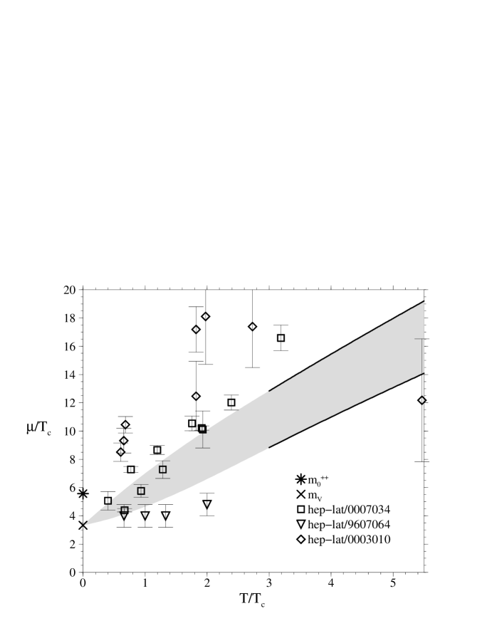
Figure 2: Temperature dependence of the screening mass in the heavy monopole potential (8). Shaded region denotes the theoretical prediction, Eqs. (11), (12-15). Symbols denote: ${\tt\times}$ – the dual gluon mass $m_{V}\approx 1GeV$ as reported in Ref. [15]; * – the mass of the lightest $0^{++}$ glueball [19]; ${\bigtriangledown}$ – magnetic screening mass measured in Maximal Abelian gauge, Ref. [12]; $\Diamond$ and $\Box$ – the screening masses measured at various temperatures in Ref. [2] and Ref. [3] respectively.

The triangles on Figure 1 denote the results of Ref. [12] obtained in the Maximal Abelian projection using the method described in the previous Section. At small temperatures these results are quantitatively in agreement with Refs. [2, 3] while at higher temperatures the screening mass obtained in Ref. [12] falls essentially lower than is indicated by the measurements in the full gluodynamics [2, 3]. It is worth emphasizing that the calculations [12] took into account only the Coulomb-like interaction between the monopoles. As is explained in the preceding section, this is justified at very low and very high temperatures, but not at the intermediate temperatures. This observation allows to understand why the results of [2, 3] and [12] agree at $T=0$ and tend to disagree at intermediate temperatures.

Conclusion

To summarize, the heavy monopole potential at small distances is of the Coulomb type with a known overall normalization. The large–distance potential is of the Yukawa type. The descent of the interaction at large distances and at non–zero temperatures is qualitatively consistent with the monopole dominance model. Thus the monopole dominance model of SU(2) gluodynamics based on the dual superconductivity predicts the inter monopole potential which is consistent with the numerical data both at small and large distances at high as well as at low temperatures. Further data are desired to allow for a detailed quantitative comparison.

References

- [1] G. ’t Hooft, Nucl. Phys. B138 (1978) 1.
- [2] C. Hoelbling, C. Rebbi and V. A. Rubakov, hep-lat/0003010. Nucl. Phys. Proc. Suppl. 83 (2000) 485, [hep-lat/9909023]; Nucl. Phys. Proc. Suppl. 73 (1999) 527, [hep-lat/9809113].
- [3] Ph. de Forcrand, M. D’Elia, M. Pepe, “ A study of the ’t Hooft loop in Yang-Mills theory”, hep-lat/0007034.
- [4] M.N. Chernodub, F.V. Gubarev, M.I. Polikarpov, V.I. Zakharov, Nucl. Phys. B592 (2000) 107; [hep-th/0003138].
- [5] M.N. Chernodub, F.V. Gubarev, M.I. Polikarpov, V.I. Zakharov, “Towards Abelian- like formulation of the dual gluodynamics”, hep-th/0010265. “Magnetic monopoles, alive”, hep-th/0007135.
-
[6]
D. Zwanziger, Phys. Rev. D3 (1971) 880;
R.A. Brandt, F. Neri, D. Zwanziger, Phys. Rev. D19 (1979) 1153. - [7] S. Coleman, in “The Unity of the Fundamental Interactions”, Erice lectures (1981), ed. A. Zichichi (Plenum, London, 1983), p. 21.
- [8] G.J. Goebel, M.T. Thomas, Phys. Rev. D30 (1984) 823.
- [9] R. Akhoury, V.I. Zakharov, Phys. Lett. B 438 (1998) 165, [hep-ph/9710487].
-
[10]
F.V. Gubarev, M.I. Polikarpov, V.I. Zakharov, Phys. Lett. B 438 (1998) 147,
[hep-th/9805175];
Mod. Phys. Lett. A14 (1999) 2039, [hep-th/9812030];
”Physics of the Power Corrections in QCD”, hep-ph/9908292;
M.N. Chernodub, F.V. Gubarev, M.I. Polikarpov, V.I. Zakharov, Phys. Lett. B 475 (2000) 303, [hep-ph/0003006]. - [11] S. Samuel, Nucl. Phys. B214 (1983) 532.
- [12] J.D. Stack, Nucl. Phys. Proc. Suppl. 53 (1997) 524, [hep-lat/9607064].
- [13] G. ’t Hooft, Nucl. Phys. B 153 (1979) 141.
-
[14]
M. Baker, J.S. Ball, F. Zachariasen,
Phys. Rep. 209 (1991) 73;
Phys. Rev. D 51 (1995) 1968;
N. Brambilla, A. Vairo, “Quark confinement and the hadron spectrum”, hep-ph/9904330. - [15] F.V. Gubarev, E.M. Ilgenfritz, M.I. Polikarpov, T. Suzuki, Phys. Lett. B 468 (1999) 134, [hep-lat/9909099].
- [16] E.V. Shuryak, “Probing the boundary of the non-perturbative QCD by small size instantons”, hep-ph/9909458.
- [17] V. Bornyakov, R. Grigorev, Nucl. Phys. Proc. Suppl. 30 (1993) 576.
- [18] U.M. Heller, F. Karsch, J. Rank, Phys. Lett. B355 (1995) 511; [hep-lat/9505016].
- [19] M. Teper,”Glueball masses and other physical properties of gauge theories in : a review of lattice results for theorists”, hep-th/9812187.
- [20] G.S. Bali, K. Schilling, J. Fingberg, U.M. Heller, F. Karsch, Int. J. Mod. Phys. C4 (1993) 1179; Phys. Rev. Lett. 71 (1993) 3059.
- [21] A. Tanaka and H. Suganuma, ”Dual Wilson loop and infrared monopole condensation in lattice QCD in the maximally Abelian gauge”, hep-lat/9901022.
-
[22]
H. Shiba and T. Suzuki,
Phys. Lett. B333 (1994) 461;
J. D. Stack, S. D. Neiman and R. J. Wensley, Phys. Rev. D50 (1994) 3399. -
[23]
A. S. Kronfeld, M. L. Laursen, G. Schierholz and U. J. Wiese,
Phys. Lett. B198 (1987) 516;
A. S. Kronfeld, G. Schierholz and U. J. Wiese, Nucl. Phys. B293 (1987) 461. -
[24]
M. N. Chernodub, S. Fujimoto, S. Kato, M. Murata, M. I. Polikarpov and T. Suzuki,
Phys. Rev. D62 (2000) 094506
[hep-lat/0006025];
M. N. Chernodub, S. Kato, N. Nakamura, M. I. Polikarpov and T. Suzuki, “Various representations of infrared effective lattice SU(2) gluodynamics”, hep-lat/9902013. -
[25]
P. Becher and H. Joos,
Z. Phys. C15 (1982) 343;
A. H. Guth, Phys. Rev. D21 (1980) 2291. - [26] J. Smit and A. van der Sijs, Nucl. Phys. B355 (1991) 603.
-
[27]
T. L. Ivanenko, A. V. Pochinsky and M. I. Polikarpov,
Phys. Lett. B302 (1993) 458;
G. Damm and W. Kerler, Phys. Lett. B397 (1997) 216 [hep-lat/9702012]. - [28] Ph. de Forcrand, private communications.