Thermalization in a Hartree Ensemble Approximation to Quantum Field Dynamics

Abstract

For homogeneous initial conditions, Hartree (gaussian) dynamical approximations are known to have problems with thermalization, because of insufficient scattering. We attempt to improve on this by writing an arbitrary density matrix as a superposition of gaussian pure states and applying the Hartree approximation to each member of such an ensemble. Particles can then scatter via their back-reaction on the typically inhomogeneous mean fields. Starting from initial states which are far from equilibrium we numerically compute the time evolution of particle distribution functions and observe that they indeed display approximate thermalization on intermediate time scales by approaching a Bose-Einstein form. However, for very large times the distributions drift towards classical-like equipartition.

I Introduction

Non-perturbative computations in quantum field theory in real time are important for our understanding of the physics of the early universe as well as dynamics of heavy ion collisions. Real-time simulations may also give us a new handle on the difficult problem of computations at finite chemical potential, e.g. in QCD. Incorporating finite density does not necessarily pose extra problems of principle, so taking time averages in a thermalized ergodic system will provide us with microcanonical expectation values.

The classical approximation has given very useful results for the sphaleron rate (see [1] and [2] for the status in three and one spatial dimensions), thermalization after preheating [3], non-equilibrium electroweak baryogenesis [4], as well as for studies of equilibration and thermalization [5, 6, 7]. With the inclusion of fermions it has given encouraging results for finite density simulations [8]. However, it suffers from Rayleigh-Jeans divergences. To some extent these can be ameliorated in scalar field theories [9], but for gauge theories the problems are more severe [10, 11]. Large $n$ approximations have also been used for initial value problems, with $O(n)$-type models. The leading order in $1/n$ has given useful results for the description of preheating dynamics in the early universe (see e.g. [12] and references therein) and for the possibly disoriented chiral condensate in heavy ion collisions [13], but it is generally considered to contain insufficient scattering for describing thermalization at larger times. This will be improved in next order in $1/n$, where scattering comes into play, but full implementation in field theory is hard. Furthermore, within quantum mechanics one finds instabilities [14, 15], and it has been argued that systematically correcting in $1/n$ does not prevent the approximation to break down at times of order $\sqrt{n}$ [16]. On the other hand, Schwinger-Dyson-like approaches including scattering diagrams appear to give more favorable results [17] and have been found to lead to equilibration in field theory [18].

The leading order large $n$ equations for the $O(n)$ model are almost identical to the Hartree approximation for the single component scalar field, and so the latter approximation is also not considered to be able to describe thermalization. Yet, in this paper we shall present evidence for approximate thermalization using Hartree dynamics in a toy model, the $\varphi^{4}$ model in 1+1 dimensions. The crucial difference with previous studies is that our system is allowed to be arbitrarily inhomogeneous. This has the effect that particle-like excitations can scatter through the intermediary of a mean field fluctuating in time and space, which in turn is created by the particles. (We used ‘Hartree’ rather than ‘large $n$’ to avoid problems with would-be Goldstone bosons in 1+1 dimensions.)

The Hartree approximation describes the dynamics in terms of a mean field and a two-point correlation function. It corresponds to a gaussian density matrix in field space, centered around the mean field with a width given by the two-point function (see e.g. [15]). The two-point function can be conveniently described in terms of a complete set of mode functions. For a homogeneous initial state the mean field is homogeneous and the mode functions can conveniently be taken in the form of plane waves labeled by a wave vector ${\bf k}$. Typically, only mode functions in a narrow $|{\bf k}|$-band get excited by the time-dependent homogeneous mean field, through parametric resonance or spinodal instability. The system equilibrates but does not thermalize in this approximation and particle distribution functions show resonance peaks instead of approaching the Bose-Einstein distribution (see for example [19]).

It is instructive to compare with the classical approximation. Simulations in this case indicate no problem of principle with thermalization (see  [5, 6, 7] for quantitative studies). Starting from an initial ensemble of classical field configurations $\rho_{c}[\varphi,\pi,t_{\rm in}]$ (with canonical field variables $\varphi$ and $\pi$), suitable observables are found to become distributed according to the classical canonical distribution $\exp(-\beta H[\varphi,\pi])$. This distribution will not be reached starting with strictly homogeneous realizations, because then the dynamics is that of a simple system with only two degrees of freedom, i.e. the spatially constant $\varphi$ and $\pi$. As initial conditions aiming at thermalization these are unsuitable realizations, even if $\rho_{c}[\varphi,\pi,t_{\rm in}]$ is homogeneous. The phase space distribution $\rho_{c}[\varphi,\pi,t_{\rm in}]$ may be homogeneous, but realizations $\varphi({\bf x},t_{\rm in})$, $\pi({\bf x},t_{\rm in})$ are typically inhomogeneous. Viewing the Hartree approximation as a semiclassical improvement, we may expect that thermalization will improve if some analogies of classical realizations are used as initial states.

To implement the idea, we note that an arbitrary density operator can be formally written as a superposition of gaussian pure states:

$$\hat{\rho}=\int[d\varphi\,d\pi]\,\rho_{q}[\varphi,\pi]\,|\varphi,\pi\rangle\langle\varphi,\pi|.$$ (1)

Here the $|\varphi,\pi\rangle$ are coherent states centered around $\varphi({\bf x})=\langle\varphi,\pi|\hat{\varphi}({\bf x})|\varphi,\pi\rangle$ and $\pi({\bf x})=\langle\varphi,\pi|\hat{\pi}({\bf x})|\varphi,\pi\rangle$, and $\rho_{q}[\varphi,\pi]$ is a functional representing the density operator $\hat{\rho}$. We interpret the $|\varphi,\pi\rangle\langle\varphi,\pi|$ as ‘realizations’ of $\hat{\rho}$. The distribution $\rho_{q}[\varphi,\pi]$ can be quite singular for non-classical states, but for suitable semiclassical states or thermal states it is positive and intuitively attractive [20]. We give a brief review in appendix A.

A thermal state like $\exp[-\beta\hat{H}]$ cannot be approximated very well by a gaussian if there are nontrivial interactions. For example, with a double well potential there are in general multiple peaks in the field distribution, while a gaussian has a single peak. But if in the decomposition (1) a gaussian state $|\varphi,\pi\rangle\langle\varphi,\pi|$ has a reasonable weight, we can take it as an initial state and use the Hartree approximation to compute the time evolution. We can then compute time averages (as long as the approximation is good), and finally sum over initial states according to (1). Such a description is semiclassical in so far as the mean field describes a near-classical path and $\rho_{q}[\varphi,\pi]$ is positive. But note that in the Hartree approximation the gaussian fluctuations (the modes comprising the two-point function – these are the ‘particle-like excitations’ alluded to above) influence the ‘classical’ field, i.e. the mean field of the ‘realization’.

For thermal equilibrium the functional $\rho_{q}[\varphi,\pi]$ is time-independent but it is not known for interacting systems. If the time evolution could be followed exactly, we would be able to reconstruct its microcanonical version, assuming the system is sufficiently strongly ergodic. With exact dynamics we can imagine starting from some initial $\rho_{q}[\varphi,\pi]$ which is reasonably close to the target distribution, wait for equilibration and subsequently compute time averages over an arbitrarily long time span. With only an approximation to the dynamics (Hartree) the distribution may deteriorate after some time and we may have to stop and start again.

Crucial questions are now, does the system equilibrate sufficiently in the Hartree approximation, such that results are insensitive to reasonable choices of the initial $\rho_{q}[\varphi,\pi]$? Does it thermalize approximately, e.g. do one-particle distribution functions get the appropriate thermal forms? How long does it take for the approximation to break down? And if the answers to these questions are sufficiently favorable, can we obtain a reasonable approximation to the target equilibrium distribution at intermediate times starting with a convenient initial one?

We study these issues in a simple model, 1+1 dimensional $\varphi^{4}$ theory. Sect. 2 introduces the model and the gaussian approximation. An effective hamiltonian $H_{\rm eff}$ describing the gaussian dynamics is introduced in Sect. 3. In Sect. 4 we discuss vacuum and thermal stationary state solutions. We note one of the flaws of the Hartree approximation, the fact that it predicts a first order phase transition where there should only be a cross-over (in 3+1 D one also gets a first order transition [21] instead of the expected second order; the inconsistency problem with coupling constant renormalization [21] is absent in 1+1 dimensions). Numerical results for the evolution from initial out-of-equilibrium distributions are presented in Sec. VI. We introduce a one particle distribution function $n_{k}(t)$ and compare its time-dependent form with the Bose-Einstein distribution. In Sect. VII we study correlations in time of the zero momentum mode of the mean field, use them for estimating damping times. The results are discussed in Sect. VIII. In appendix A we discuss the representation (1), in B classical equipartition according to $H_{\rm eff}$.

II Gaussian approximation

We start with the Heisenberg field equation for the quantum field at times $x^{0}>0$,

$$(-\partial^{2}+\mu^{2})\hat{\varphi}(x)+\lambda\hat{\varphi}(x)^{3}=0.$$ (2)

For exact evaluation we would have to specify the infinite set of matrix elements of $\hat{\varphi}({\bf x},0)$ and $\partial_{0}\hat{\varphi}({\bf x},0)$ as initial conditions. In practise, of course, less detail is needed. Taking the expectation value in an initial state at time $x^{0}=0$ leads to

$$\langle\hat{\varphi}(x)\rangle = \varphi(x),$$ (3)

$$\langle T\hat{\varphi}(x_{1})\hat{\varphi}(x_{2})\rangle = \varphi(x_{1})\varphi(x_{2})-iG(x_{1},x_{2}),$$ (4)

$$\langle T\hat{\varphi}(x_{1})\hat{\varphi}(x_{2})\hat{\varphi}(x_{3})\rangle = \varphi(x_{1})\varphi(x_{2})\varphi(x_{3})-i\varphi(x_{1})G(x_{2},x_{3})+\mbox{2 perm.}$$ (6)

$$+(-i)^{2}G(x_{1},x_{2},x_{3}),$$

$$\langle T\hat{\varphi}(x_{1})\cdots\hat{\varphi}(x_{4})\rangle = \varphi(x_{1})\cdots\varphi(x_{4})-i\varphi(x_{1})\varphi(x_{2})G(x_{3},x_{4})+\mbox{6 perm.}$$ (10)

$$+\varphi(x_{1})(-i)^{2}G(x_{2},x_{3},x_{4})+\mbox{3 perm.}$$

$$+(-i)^{2}G(x_{1},x_{2})G(x_{3},x_{4})+\mbox{2 perm.}$$

$$+(-i)^{3}G(x_{1},\ldots,x_{4}),$$

etc. Here $T$ denotes time ordering and

$$\langle\hat{\varphi}(x_{1})\cdots\hat{\varphi}(x_{n})\rangle\equiv\mbox{Tr}\,\hat{\rho}\,\hat{\varphi}(x_{1})\cdots\hat{\varphi}(x_{n}),$$ (11)

with $\hat{\rho}$ the initial density operator; $\varphi$ is the mean field (or classical field) and the $G^{\prime}s$ are correlation functions (connected Green functions). Taking the expectation value of (2) and neglecting the three point correlation function $G(x,x,x)$ gives the approximate equation

$$[-\partial^{2}+\mu^{2}+\lambda\varphi(x)^{2}-3i\lambda G(x,x)]\varphi(x)=0.$$ (12)

To use it we need an equation for the two-point function. Such an equation can be found by multiplying (2) by $\hat{\varphi}(y)$ and taking again the expectation value in the initial state. This leads to the approximate equation

$$[-\partial^{2}+\mu^{2}+3\lambda\varphi(x)^{2}-3i\lambda G(x,x)]\,G(x,y)=\delta^{4}(x-y),$$ (13)

where we used the canonical commutation relations and dropped the three and four-point correlation functions. We shall comment on their neglect at the end of this section. Since only the two-point function appears, Eqs. (12,13) are exact if the hamiltonian and density matrix are approximated by gaussian forms. Given the neglect of the higher correlation functions the initial density matrix does not have to be gaussian per se, but its non-gaussianity does not enter in Eqs. (12,13). For clarity we shall now assume the bra-kets $\langle\cdots\rangle$ to refer to a gaussian density operator $\rho$. Later we will consider non-gaussian operators by further averaging over initial conditions, as in (1), which will be indicated by $\overline{\langle\cdots\rangle}$.

An intuitive as well as practical way for computing the two-point function is in terms of mode functions $f_{\alpha}(x)$. We write

$$-iG(x,y)=\theta(x^{0}-y^{0})C(x,y)+\theta(y^{0}-x^{0})C(y,x).$$ (14)

such that

$$C(x,y)=\langle[\hat{\varphi}(x)-\varphi(x)][\hat{\varphi}(y)-\varphi(y)]\rangle.$$ (15)

It follows from (13) that $C(x,y)$ satisfies the homogeneous equation ($\delta^{4}(x-y)\to 0$), in the variable $x$ as well as in $y$, as if $\hat{\varphi}(x)-\varphi(x)$ satisfies this equation. We can now introduce mode functions $f_{\alpha}(x)$ satisfying the homogeneous equation,

$$[-\partial^{2}+\mu^{2}+3\lambda\varphi(x)^{2}+3\lambda C(x,x)]\,f_{\alpha}(x)=0,$$ (16)

($-iG(x,x)=C(x,x)$) and write

$$\hat{\varphi}(x)\stackrel{{\scriptstyle\rm g.a.}}{{=}}\varphi(x)+\sum_{\alpha}\left[\hat{b}_{\alpha}f_{\alpha}(x)+\hat{b}^{\dagger}_{\alpha}f_{\alpha}^{*}(x)\right].$$ (17)

where the $\hat{b}_{\alpha}$ and $\hat{b}^{\dagger}_{\alpha}$ are spacetime independent and ‘g.a.’ means ‘gaussian approximation’. The wave equation (16) for the $f_{\alpha}$ is of the Klein-Gordon type and we require the mode functions to be orthogonal and complete in the Klein-Gordon sense,

$$\int d^{3}x\,\left[f_{\alpha}^{*}(x)i\partial_{0}f_{\beta}(x)-i\partial_{0}f_{\alpha}^{*}(x)f_{\beta}(x)\right] = \delta_{\alpha\beta},$$ (18)

$$\int d^{3}x\,\left[f_{\alpha}(x)i\partial_{0}f_{\beta}(x)-i\partial_{0}f_{\alpha}(x)f_{\beta}(x)\right] = 0,$$ (19)

$$\sum_{\alpha}\left[-if_{\alpha}(x)\partial_{0}f_{\alpha}^{*}(y)+if_{\alpha}^{*}(x)\partial_{0}f_{\alpha}(y)\right]_{x^{0}=y^{0}} = \delta^{3}({\bf x}-{\bf y}),$$ (20)

$$\sum_{\alpha}\left[f_{\alpha}(x)f_{\alpha}^{*}(y)-f_{\alpha}^{*}(x)f_{\alpha}(y)\right]_{x^{0}=y^{0}} = 0,$$ (21)

$$\sum_{\alpha}\left[\partial_{0}f_{\alpha}(x)\partial_{0}f_{\alpha}^{*}(y)-\partial_{0}f_{\alpha}^{*}(x)\partial_{0}f_{\alpha}(y)\right]_{x^{0}=y^{0}} = 0.$$ (22)

The above orthogonality and completeness relations are preserved by the equation of motion (16) for the $f_{\alpha}$. The canonical commutation relations for $\hat{\varphi}$ and $\partial_{0}\hat{\varphi}$ translate into

$$[\hat{b}_{\alpha},\hat{b}^{\dagger}_{\beta}]=\delta_{\alpha\beta},\;\;\;\;[\hat{b}_{\alpha},\hat{b}_{\beta}]=[\hat{b}^{\dagger}_{\alpha},\hat{b}^{\dagger}_{\beta}]=0.$$ (23)

The initial condition implies $\langle\hat{b}_{\alpha}\rangle=0$ and we have to specify $E_{\alpha\beta}\equiv\langle\hat{b}_{\alpha}\hat{b}_{\beta}\rangle$ and $N_{\alpha\beta}\equiv\langle\hat{b}^{\dagger}_{\alpha}\hat{b}_{\beta}\rangle$. The matrices $N$ and $E$ are subject to constraints following from their definition as expectation values of operators in Hilbert space. We shall assume that a Bogoliubov transformation $\hat{b}_{\alpha}\to\sum_{\beta}[A_{\alpha\beta}\hat{b}_{\beta}+B_{\alpha\beta}\hat{b}^{\dagger}_{\beta}]$ can be made such that $E_{\alpha\beta}\to 0$ and $N_{\alpha\beta}\propto\delta_{\alpha\beta}$. This transformation produces new mode functions which are linear combinations of the $f$ and $f^{*}$. In the new basis we only have to specify as initial conditions

$$\langle\hat{b}^{\dagger}_{\alpha}\hat{b}_{\beta}\rangle\equiv n^{0}_{\alpha}\,\delta_{\alpha\beta},\;\;\;\;n^{0}_{\alpha}\geq 0,$$ (24)

in terms of which

$$C(x,y)=\sum_{\alpha}\left[(1+n^{0}_{\alpha})f_{\alpha}(x)f_{\alpha}^{*}(y)+n^{0}_{\alpha}f_{\alpha}^{*}(x)f_{\alpha}(y)\right].$$ (25)

Eq. (17) expresses the fact that in the gaussian approximation the field $\hat{\varphi}^{\prime}(x)\equiv\hat{\varphi}(x)-\varphi(x)$ is a generalized free field, i.e. its correlation functions are completely determined by the two-point function. Its linear field equation (i.e. (16) with $f_{\alpha}\to\hat{\varphi}^{\prime}$) is equivalent to the Heisenberg equations of motion of the effective gaussian hamiltonian operator

$$\hat{H}_{\rm g.a.}=\int d^{3}x\,\left[\frac{1}{2}\hat{\pi}^{\prime 2}+\frac{1}{2}(\nabla\hat{\varphi}^{\prime})^{2}+\frac{1}{2}m_{\rm eff}^{2}\hat{\varphi}^{\prime 2}+\epsilon_{\rm eff}\right],$$ (26)

where the spacetime dependent effective mass $m^{2}_{\rm eff}$ is given by

$$m_{\rm eff}^{2}(x)=3\lambda\varphi(x)^{2}+3\lambda C(x,x).$$ (27)

We also introduced an effective c-number energy density $\epsilon_{\rm eff}$, which is determined by requiring $\langle\hat{H}_{\rm g.a.}\rangle=\langle\hat{H}\rangle$:

$$\epsilon_{\rm eff}(x)=\frac{1}{2}\pi(x)^{2}+\frac{1}{2}[\nabla\varphi(x)]^{2}+\frac{1}{2}\mu^{2}\varphi(x)^{2}+\frac{1}{4}\lambda\varphi(x)^{4}-\frac{3}{4}\lambda C(x,x)^{2}.$$ (28)

Summarizing, the gaussian approximation consists of eqs. (12), (16), (24) and (25), together with the orthogonality and completeness conditions (18)-(22) for the mode functions and some initial condition for the mean field and mode functions.

The gaussian approximation can be justified in the limit of large $n$ for the $O(n)$ model. The resulting field equations are very similar: we only need to make the replacement $3\to 1$ in eqs. (12) and (16).

The above derivation in terms of the Heisenberg equations of motion can be put into the systematic framework of the Dyson-Schwinger hierarchy. These equations follow from functionally differentiating an exact equation of motion $\delta\Gamma/\delta\varphi=-J$ with respect to $J$ and setting $J=0$ afterwards. Here $\Gamma$ is the effective action (with time integration along the usual Keldysh-Schwinger contour) and $J$ an external source. We shall not go into details here, but just comment on the systematics, using diagrams (for a derivation, see e.g. [22]). Fig. 1 illustrates the exact equation for the mean field. The gaussian approximation (12) is obtained by dropping the two-loop diagram. By differentiating the diagrams in Fig. 1 we get the exact equation for the two-point correlation function illustrated in Fig. 2. The gaussian approximation (13) can be obtained from this by: a) dropping the two-loop contributions and b) dropping the second one-loop diagram. The neglect of the two-loop terms may be reasonable at weak coupling, and even the second approximation may be justifiable if the product of the three point couplings (one bare, the other dressed) is substantially smaller than the (bare) four point coupling in the first one-loop diagram. However, since the bare three point vertex $\delta^{3}S/\delta\varphi^{3}\propto\lambda\varphi$ we see that this is not likely if $\varphi=O(\lambda^{-1/2})$ or larger. Especially this second approximation b) is worrisome, because on iteration of the integral equations we would not get correctly all one-loop diagrams. It is also known that the approximation does not give exact Goldstone bosons where one expects them, because the phase transition is incorrectly predicted to be first order, instead of second order (in 3+1 D) or a cross over (1+1 D). There is a problem with renormalization in 3+1 dimensions [21] (but not in 1+1 D).

It will depend on the circumstances if these troublesome features of the Hartree approximation are numerically important.

III Effective hamiltonian and conserved charges

The equations of the gaussian approximation derived in section II are local in time and they may be derived from a conserved effective hamiltonian. We shall present it here and exhibit its symmetries and accompanying conserved charges. We write

$$f_{\alpha}(x) = \frac{1}{\sqrt{2}}\left[f_{\alpha 1}(x)-if_{\alpha 2}(x)\right],$$ (29)

$$\xi_{\alpha a}(x) = \left(\frac{1}{2}+n^{0}_{\alpha}\right)^{1/2}f_{\alpha a}(x),\;\;\;\;a=1,2.$$ (30)

$$\eta_{\alpha a}(x) = \partial_{0}\xi_{\alpha a}(x),\;\;\;\;\pi(x)=\partial_{0}\varphi(x).$$ (31)

In terms of the real canonical variables $\varphi$, $\pi$, $\xi_{\alpha a}$ and $\eta_{\alpha a}$ the effective hamiltonian takes the form

$$H_{\rm eff} = \int d^{3}x\,\left[\frac{1}{2}\left(\pi^{2}+\eta^{2}+(\nabla\varphi)^{2}+(\nabla\xi)^{2}\right)\right.$$ (33)

$$\left.\mbox{}+\frac{1}{2}\mu^{2}\left(\varphi^{2}+\xi^{2}\right)+\frac{1}{4}\lambda\left(\varphi^{4}+6\varphi^{2}\xi^{2}+3(\xi^{2})^{2}\right)\right],$$

where

$$\xi^{2}=\sum_{\alpha}\left(\xi_{\alpha 1}^{2}+\xi_{\alpha 2}^{2}\right),\;\;\;(\nabla\xi)^{2}=\sum_{\alpha}\left[(\nabla\xi_{\alpha 1})^{2}+(\nabla\xi_{\alpha 2})^{2}\right],\;\;\;\eta^{2}=\sum_{\alpha}\left(\eta_{\alpha 1}^{2}+\eta_{\alpha 2}^{2}\right).$$ (34)

It is easy to check that the mean field equation (12) and the mode equations (16) are equivalent to the Hamilton equations

$$\partial_{0}\varphi=\pi,\;\;\;\partial_{0}\pi=-\frac{\delta H_{\rm eff}}{\delta\varphi},\;\;\;\;\partial_{0}\xi_{\alpha a}=\eta_{\alpha a},\;\;\;\;\partial_{0}\eta_{\alpha a}=-\frac{\delta H_{\rm eff}}{\delta\xi_{\alpha a}}.$$ (35)

It is also straightforward to show that $H_{\rm eff}$ is just the expectation value of the quantum hamiltonian $\hat{H}(t)$ upon inserting the gaussian approximation (17),

$$H_{\rm eff}=\langle\hat{H}\rangle.$$ (36)

The effective hamiltonian has evidently a large symmetry corresponding to rotations of the infinite dimensional vectors $\xi_{\alpha a}$ and $\eta_{\alpha a}$. For definiteness, let us assume a regularization of the field theory such that there are $M$ modes, $\alpha=1,\ldots,M$ (e.g. on an $N^{3}$ periodic lattice $M=N^{3}$). Then the effective hamiltonian has $O(2M)$ symmetry, implying $M(2M-1)$ conserved generalized angular momenta of the general form

$$L_{\alpha a,\beta b}=\int d^{3}x\,\left(\xi_{\alpha a}\eta_{\beta b}-\xi_{\beta b}\eta_{\alpha a}\right),\;\;\;(\alpha,a)\neq(\beta,b).$$ (37)

Recalling the orthonormality relations for the mode functions (18), (19) we see that the conserved quantities are given in terms of the initial conditions as

$$L_{\alpha 1,\alpha 2}=\frac{1}{2}+n^{0}_{\alpha},$$ (38)

with all others vanishing.

It is interesting to compare with the effective hamiltonian corresponding to the large $n$ limit of the $O(n)$ model [23], which may be obtained from $H_{\rm eff}$ above by the replacement $3\to 1$ (and $6\to 2$). This has the effect of producing the combination $\lambda(\varphi^{2}+\xi^{2})^{2}$, so the symmetry enlarges to $O(2M+1)$. The additional $2M$ conserved generalized angular momenta depend on the initial conditions for $\varphi$ and $\pi$.

IV Equilibrium states

In a first exploration of the system and of the gaussian approximation we study equilibrium states, i.e. stationary states with maximum entropy. This will give information on the phase structure and quasiparticle excitations as a function of temperature. From now on we specialize to 1+1 dimensions, $x^{\mu}\to(x,t)$, and assume the system to have ‘volume’ $L$ with periodic boundary conditions. The coupling $\lambda$ needs no renormalization while the bare mass parameter $\mu^{2}$ is only logarithmically divergent with the implicit cutoff.

We assume the equilibrium states to be homogeneous and time-independent, i.e. $\varphi(x,t)=v$ and $C(x,t;y,t)=C(x-y,0;0,0)$. Also the various time derivatives of $C$ evaluated at equal times are assumed to be time-independent. We shall seek solutions of the form (25) in which the mode functions are plane waves,

$$\varphi(x,t)=v,\;\;\;\;f_{k}(x,t)=\frac{e^{ikx-i\omega_{k}t}}{\sqrt{2\omega_{k}L}}.$$ (39)

Here the label $\alpha$ is the wave number $k$ and we write $n_{k}$ for the corresponding (time independent) occupation numbers. With this ansatz the equations for the mean field and mode functions reduce to

$$(\mu^{2}+3\lambda C+\lambda v^{2})v = 0,$$ (40)

$$-\omega_{k}^{2}+k^{2}+\mu^{2}+3\lambda C+3\lambda v^{2} = 0,$$ (41)

where $C=C(x,t;x,t)$ is time-independent. In the infinite volume limit it is given by

$$C=\int\frac{dk}{2\pi}\,\left(n_{k}+\frac{1}{2}\right)\,\frac{1}{\omega_{k}}.$$ (42)

It follows that

$$\omega_{k}^{2}=m^{2}+k^{2},\;\;\;\;m^{2}=\mu^{2}+3\lambda C+3\lambda v^{2}.$$ (43)

To determine the $n_{k}$ we maximize the entropy $S$ subject to the constraint of fixed energy $U\equiv H_{\rm eff}=E$, i.e. maximize $S+\beta(E-U)$, with Lagrange multiplyer $\beta$. We shall write these equations in terms of the densities $s=S/L$, $u=U/L$, $\epsilon=E/L$ with $L\to\infty$. The (unrenormalized) energy density $u$ is given by

$$u=\frac{H_{\rm eff}}{L}=\frac{1}{2}\mu^{2}v^{2}+\frac{1}{4}\lambda v^{4}+\int\frac{dk}{2\pi}\,\left(n_{k}+\frac{1}{2}\right)\frac{\omega_{k}^{2}+k^{2}+\mu^{2}+3\lambda v^{2}}{2\omega_{k}}+\frac{3}{4}\,\lambda C^{2},$$ (44)

and for our gaussian density operator, $s$ can be written as

$$s=-\frac{1}{L}\mbox{Tr}\,\rho\log\rho=\int\frac{dk}{2\pi}\,\left[\left(n_{k}+1\right)\log\left(n_{k}+1\right)-n_{k}\log n_{k}\right].$$ (45)

The maximization equations read

$$0=\frac{\delta[s+\beta(\epsilon-u)]}{\delta n_{k}}=\log\left(\frac{n_{k}+1}{n_{k}}\right)-\beta\omega_{k},\;\;\;\;u=\epsilon,$$ (46)

with the solution

$$n_{k}=\frac{1}{e^{\beta\omega_{k}}-1}$$ (47)

and $\beta$ such that $u=\epsilon$. So we found equilibrium states of the Hartree evolution corresponding to the Bose-Einstein distribution with temperature $T=\beta^{-1}$. All effects of the interaction are buried in the temperature dependent mass $m$ introduced in (43).

For simplicity of discussion, let us next use a simple momentum cutoff $|k|<\Lambda$ and define a renormalized mass parameter $\mu_{r}^{2}$ by

$$\mu_{r}^{2}=\mu^{2}+\frac{3\lambda}{4\pi}\log\frac{4\Lambda^{2}}{\lambda}.$$ (48)

Then (43) takes the renormalized form

$$m^{2}=\mu_{r}^{2}+\frac{3\lambda}{4\pi}\log\frac{\lambda}{m^{2}}+3\lambda\int_{0}^{\infty}\frac{dk}{\pi}\,\frac{1}{\sqrt{m^{2}+k^{2}}}\,\frac{1}{e^{\sqrt{m^{2}+k^{2}}/T}-1}+3\lambda v^{2}.$$ (49)

At zero temperature the equilibrium state is the vacuum. For $v=0$ there is one solution $m^{2}$ for every $\mu_{r}^{2}\in(-\infty,\infty)$. For nonzero $v$ we get with (40) the relations

$$m^{2}=2\lambda v^{2},\;\;\;\;\mu_{r}^{2}=-\frac{1}{2}m^{2}+\frac{3\lambda}{4\pi}\log\frac{m^{2}}{\lambda}.$$ (50)

There turn out to be two solutions, provided $\mu_{r}^{2}/\lambda<(3/4\pi)[-1+\log(3/2\pi)]\approx-0.415$, otherwise none. To determine the true ground state we plot in Fig. 3 the effective potential $u$ as a function $\varphi$ (i.e. $m^{2}$ is the solution of (49) with $v\to\varphi$ at $T=0$), for various $\mu_{r}$. The plot shows that there is a first order phase transition as a function of $\mu_{r}^{2}$, instead of the expected second order transition for a model in the universality class of the Ising model. This mis-representation of the phase transition is a well-known artefact of the gaussian approximation (see, e.g. [21]).

Note that the 2nd order transition would occur at strong coupling $\lambda/m^{2}\to\infty$, where the gaussian approximation is suspect. In fact, the two masses at the transition also imply strong coupling: they are given by $\lambda/m^{2}\approx 10$, for $\varphi=0$ and $\lambda/m^{2}\approx 1.2$ for $\varphi=v_{c}\approx 0.65$. To avoid fake first order effects we should evidently choose parameters away from the transition region. For this paper we mostly used $\lambda/m^{2}=1/12$ for which there is only one ground state at $v^{2}=6$, well away from $v_{c}^{2}\approx 0.65$.

Having determined the groundstate we define the renormalized energy $H_{\rm eff,r}$ by subtracting from $H_{\rm eff}$ its value in the ground state, such that the vacuum energy is zero. It can be instructive to split the total energy into a classical (gaussian mean field) part and a mode energy, $H_{\rm eff,r}=H_{\rm clas}+H_{\rm modes}$, where we define the classical part as

$$H_{\rm clas} = \int dx\,\left[\frac{1}{2}\pi^{2}+\frac{1}{2}(\nabla\varphi)^{2}+V_{\rm clas}(\varphi)\right],$$ (51)

$$V_{\rm clas}(\varphi) = \frac{1}{2}m^{2}\varphi^{2}+\frac{1}{4}\lambda\varphi^{4},\;\;\;\;v=0,$$ (52)

$$= \frac{1}{4}\lambda\left(\varphi^{2}-v^{2}\right)^{2},\;\;\;\;v\neq 0,$$ (53)

where $m^{2}$ and $v^{2}$ are the vacuum values ($T=0$).

Consider now starting in the broken symmetry phase $v\neq 0$ at zero temperature and raising the temperature. In 1+1 dimensions there should be only a cross over and not a true phase transition. Fig. 4 shows the finite temperature effective potential (free energy density)

$$f(\varphi)=u(\varphi)-Ts(\varphi),$$ (54)

using the temperature $T$ as independent variable instead of the energy density $\epsilon$. Now $m^{2}=m^{2}(\varphi,T)$ is the solution of (49), $v\to\varphi$, at finite $T$. The parameters were chosen such that $v^{2}=m^{2}(v,0)/2\lambda=6$ at $T=0$. We see again a fake first order transition, at $T_{c}\approx 1.79\,m(v,0)$, with $v_{c}=1.96$. Its latent heat $\ell$ and surface tension $\sigma$ are given by $\ell=\Delta u=0.39\,m(v,0)^{2}$, $\sigma=\int_{0}^{v_{c}}d\varphi\,\sqrt{2f(\varphi)}=0.295\,m(v,0)$. These are not particularly small values and we may not argue that the effects of the first order transition will be negligible under generic circumstances. However, the critical size of a nucleating bubble is zero in 1+1 dimensions, so the bubble nucleation rate is not suppressed ($\propto\exp(-2\sigma/T_{c})\approx\exp(-0.17)$) and supercooling will not be strong.

We end this section with some cautionary remarks. First, the fact that the equilibrium correlation function $C(x,y)$ has the free form (i.e. eq. (56) below with $n_{k}$ given by the Bose-Einstein form (47)) for any coupling strength is a result of the gaussian approximation. The exact correlation function will have a more complicated form, although the corrections are expected to be small at weak coupling. We will check this by a Monte Carlo computation in a separate publication [25].

Second, it is not clear that the finite temperature equilibrium state found above will actually be approached at very large times. Any set of numbers $n_{k}$ in conjunction with Eqs. (39)–(44) gives a stationary solution to the Hartree equations. Our derivation of the Bose-Einstein form for $n_{k}$ used the standard form (45) for the entropy, but we have not shown that this entropy is a large time result of the dynamics. Of course, this would be trivially the case if we choose the initial ocupation numbers $n^{0}_{\alpha}=n_{k}$. But for a generic gaussian initial state the correlation function may still approach a fixed point of the form just discussed ($t\approx t^{\prime}$),

$$C(x,t;x^{\prime},t^{\prime}) = \sum_{\alpha}\left[(1+n^{0}_{\alpha})f_{\alpha}(x,t)f_{\alpha}^{*}(x^{\prime},t^{\prime})+n^{0}_{\alpha}f_{\alpha}^{*}(x,t)f_{\alpha}(x^{\prime},t^{\prime})\right]$$ (55)

$$\to \int\frac{dk}{2\pi}\,\left[\frac{1+n_{k}}{2\omega_{k}}\,e^{ik(x-x^{\prime})-i\omega_{k}(t-t^{\prime})}+\frac{n_{k}}{2\omega_{k}}\,e^{-ik(x-x^{\prime})+i\omega_{k}(t-t^{\prime})}\right],$$ (56)

where the $n_{k}$ are expected to correspond to maximum entropy in relation to the dynamics. Since the Hartree dynamics in terms of $H_{\rm eff}$ is classical we may expect this entropy to take a classical form, which would lead to

$$n_{k}=\frac{T}{\omega_{k}}.$$ (57)

Matters are complicated by the presence of the infinitely many conserved charges (38), which are determined by the initial conditions. Note that without these constraints one would expect $n_{k}+1/2=T/\omega_{k}$, instead of (57), which makes a big difference because equipartition suggests low $T=O(\epsilon/\Lambda)$ and therefore small $n_{k}$. We elaborate on this in appendix B.

To study such matters numerically we now first introduce a coarse graining of the correlation function and define a corresponding time dependent distribution function $n_{k}(t)$.

V Coarse grained particle numbers

The mode functions may be interpreted as representing particles which interact through the mean field. This is similar to electrons scattering off each other in classical electrodynamics, albeit that here the ‘particles’ are treated quantum mechanically and their interaction is short ranged. Intuitively, such an interpretation supposes that the particles are localized, with a correspondingly fluctuating (and hence inhomogeneous) mean field taking the role of a classical field.

Within such a picture one expects the system to thermalize approximately. We would like such thermalization to be quantal, e.g. with particle distribution functions which are of the Bose-Einstein type. However, the fact that our equations of motion have the form of classical Hamilton equations in terms of $H_{\rm eff}$ suggests otherwise, namely a distribution approaching a classical Boltzmann form $\exp(-\beta H_{\rm eff})$, subject to the constraints set by the large number of conserved charges (37). But this may take a very long time. In any case, one way to test the gaussian approximation is to study its thermalization properties.

This we do by looking at equal time correlation functions, coarse grained by averaging over a spacetime region. Assuming the system is weakly coupled we can compare such averages with a free field form in terms of quasiparticles with effective masses. If the system equilibrates locally in a quantum way, then the quasiparticle distribution $n_{k}$ should approach the Bose-Einstein form. We define the correlation functions

$$S(x,y,t) = \overline{\langle\hat{\varphi}(x,t)\hat{\varphi}(y,t)\rangle}-\overline{\langle\hat{\varphi}(x,t)\rangle}\;\overline{\langle\hat{\varphi}(y,t)\rangle},$$ (58)

$$T(x,y,t) = \frac{1}{2}\overline{\langle\left[\hat{\varphi}(x,t)\hat{\pi}(y,t)+\hat{\pi}(y,t)\hat{\varphi}(x,t)\right]\rangle}-\overline{\langle\hat{\varphi}(x,t)\rangle}\;\overline{\langle\hat{\pi}(y,t)\rangle},$$ (59)

$$U(x,y,t) = \overline{\langle\hat{\pi}(x,t)\hat{\pi}(y,t)\rangle}-\overline{\langle\hat{\pi}(x,t)\rangle}\;\overline{\langle\hat{\pi}(y,t)\rangle},$$ (60)

where the overbar denotes the spacetime averaging as well as a possible average over initial conditions as in (1). Using (3) and (15) we can express these quantities in terms of a ‘classical’ (mean field) and a ‘quantum’ contribution,

$$S(x,y,t) = S^{c}(x,y,t)+S^{q}(x,y,t),$$ (61)

$$S^{c}(x,y,t) = \overline{\varphi(x,t)\varphi(y,t)}-\overline{\varphi(x,t)}\;\overline{\varphi(y,t)},$$ (62)

$$S^{q}(x,y,t) = \overline{C(x,t;y,t)},$$ (63)

etc. Note that $S^{c}\to 0$ in case of averaging over initial conditions and/or spacetime.

For simplicity the spatial average is performed over all of space. For example,

$$\overline{\langle\hat{\varphi}(x,t)\hat{\varphi}(y,t)\rangle}=\frac{1}{L\Delta}\int_{t-\Delta/2}^{t+\Delta/2}dt^{\prime}\,\int_{0}^{L}dz\,\langle\hat{\varphi}(x+z,t^{\prime})\hat{\varphi}(y+z,t^{\prime})\rangle.$$ (64)

Because of the periodic boundary conditions $S$, $T$ and $U$ depend only on the difference between $x$ and $y$. Taking the Fourier transform

$$S_{k}(t)=\frac{1}{L}\int_{0}^{L}dx\,dy\,e^{-ik(x-y)}\,S(x,y,t),\;\;\;\;k=(0,\pm 1,\pm 2,\cdots)\frac{2\pi}{L},$$ (65)

and similarly for $T$ and $U$, it is easy to see that $S$ and $U$ are symmetric and positive, i.e.

$$S_{k}(t)=S_{-k}(t)\geq 0,\;\;\;\;U_{k}(t)=U_{-k}(t)\geq 0,$$ (66)

while $T_{k}$ enjoys no such properties. For a free field with average occupation numbers $\langle\hat{a}^{\dagger}_{k}\hat{a}_{k}\rangle=n_{k}$ and frequencies $\omega_{k}$ the correlators are given by $S_{k}=(n_{k}+n_{-k}+1)/2\omega_{k}$, $T_{k}=(n_{k}-n_{-k})/2$ and $U_{k}=S_{k}\omega_{k}^{2}$. Note that in this case $T$ is antisymmetric. We now define $\omega_{k}(t)$ and $n_{k}(t)$ for the interacting case by

$$n_{k}(t) = n_{k}^{s}(t)+n_{k}^{a}(t),\;\;\;\;n_{k}^{s}(t)=n_{-k}^{s}(t),\;\;\;n_{k}^{a}(t)=-n_{-k}^{a}(t),$$ (67)

$$S_{k}(t) = \left[n_{k}^{s}(t)+\frac{1}{2}\right]\frac{1}{\omega_{k}(t)},$$ (68)

$$T^{a}_{k}(t) = \frac{1}{2}\left[T_{k}(t)-T_{-k}(t)\right]=n_{k}^{a}(t),$$ (69)

$$U_{k}(t) = \left[n_{k}^{s}(t)+\frac{1}{2}\right]\,\omega_{k}(t).$$ (70)

These equations can be easily solved in terms of $\omega_{k}$ and $n_{k}$: $\omega_{k}=\omega_{-k}=\sqrt{U_{k}/S_{k}}$, $n_{k}^{s}=\omega_{k}S_{k}-1/2$ and $n_{k}$ follows by adding $T_{k}^{a}$.

There is a more direct interpretation of these formulas in terms of the expectation value of a number operator $\hat{a}^{\dagger}_{k}\hat{a}_{k}$. Suppose we define time dependent creation and annihilation operators as

$$\hat{a}_{k}(t)=\frac{1}{\sqrt{2\omega_{k}(t)L}}\int_{0}^{L}dx\,e^{-ikx}\,[\omega_{k}(t)\hat{\varphi}(x,t)+i\hat{\pi}(x,t)],\;\;\;\;\hat{a}^{\dagger}_{k}(t)=\left(\hat{a}_{k}(t)\right)^{\dagger}.$$ (71)

Then

$$\overline{\langle\hat{a}^{\dagger}_{k}(t)\hat{a}_{k}(t)\rangle}=n_{k}(t).$$ (72)

The problem with starting with (71) is that one does not know a priori how to choose the $\omega_{k}(t)$. This is especially so if some of the effective squared frequencies $\mu^{2}+3\lambda\varphi^{2}+3\lambda C$ in the equations for the mode functions turn negative. The line of reasoning leading to (67) – (70) solves this problem, but we should keep in mind that this is by brute force, which can be misleading in extreme situations, e.g. when the spectral function is not dominated by a sufficiently narrow quasiparticle bump.

VI Numerical results

We now describe some simulations used for obtaining the particle numbers $n_{k}(t)$. The mass and coupling parameters were chosen such that the system at zero temperature is in the ‘broken symmetry phase’. The coupling was weak, $v^{2}=m^{2}/2\lambda=6$. Here and in the following $m$ is the mass of the particles at zero temperature.

The system is discretized on a space-time lattice with spatial (temporal) lattice distance $a$ ($a_{0}$), with $a_{0}/a=0.1$. The number of spatial lattice sites, equal to the number of independent complex mode functions, will be denotes with $N=L/a$. The discretized lagrangian gives rise to second order difference equations, with a time evolution which is equivalent to a first order leapfrog algorithm for $\pi_{x}(t)\equiv[\varphi_{x}(t+a_{0})-\varphi_{x}(t)]/a_{0}$ and $\varphi_{x}(t)$.

The initialization is similar to that used in [5, 6],

$$\varphi_{x}=v,\qquad\pi_{x}=Am\sum_{j=1}^{j_{\rm max}}\cos(2\pi jx/L-\psi_{j}),$$ (73)

with random phases $\psi_{j}$ uniformly distributed in $[0,2\pi)$. The modes are initialized with the equilibrium form at zero temperature: the $n^{0}_{k}$ are all zero and the modes $f_{k}(x,0)$, $\dot{f}_{k}(x,0)$ are given by the plane waves (39) and its time derivative at $t=0$, with $\omega_{k}^{2}=k^{2}+m^{2}$. The density operator is thus a superposition of coherent pure states as in (1).

We now describe a simulation for which $\lambda/m^{2}=1/12$, $N=256$, $mL=32$, $j_{\rm max}=4$, $A=1/\sqrt{2}$, such that the energy density is given by $E/Lm^{2}=A^{2}j_{\rm max}/4=0.5$. A Bose-Einstein distribution describing particles with such an energy density would have a temperature $T/m\approx 1.08$, well below the phase transition at $T/m\approx 1.8$, as calculated with the finite temperature effective potential. We also chose these parameters so that the system may end up in a low temperature quantum regime and not in a classical regime with $T/m\gg 1$. A boring consequence was that the volume averaged mean field typically just oscillated around one of the two minima, we did not encounter an initial condition for which it crossed the barrier after $tm>50$.

Initially the mean field carries all the energy in its low momentum modes $0<k/m\leq\pi/4$ (zero momentum mode excluded). Due to interaction with the inhomogeneous mean field, the modes will not keep the vacuum form, but get excited. Fig. 5 shows the time dependence of the energy density for one of the members of the ensemble. The total energy is conserved up to a numerical accuracy of about 0.2%. The energy in the mean field (cf. (51) for its definition), initially equal to the total energy, is decreasing rapidly and after a time $tm\approx 100$ about 50% has been transfered to the modes. The mean field continues losing energy after that time but at a time $tm$ of the order 20000 some 15% is still left.

The development of the particle numbers $n_{k}(t)$ at early times is shown in Fig. 6, including the mean field contribution, cf. (61)–(63). Initially the mean field gives the main contribution since $n_{k}^{0}=0$ for the modes, but then the mode contribution rapidly takes over. Because the mean field contribution fluctuates strongly we used as many as 500 initial conditions for these early times, without coarsening over time. Fig. 7 shows the mode contribution to $n_{k}$ as a function of $\omega$ (40 initial conditions were used for the data at $tm>200$, with no coarsening over time). It starts out identically zero, rises rapidly and then appears to stabilize. The figure also shows a fit to the Bose-Einstein distribution with chemical potential $\mu$ at time $tm=990$. A chemical potential is expected to develop temporarily at weak coupling, since elastic scattering dominates over processes like $2\leftrightarrow 4$ scattering. The fitted temperature ($\beta m=1.08$) is already approaching the earlier estimate $T/m\approx 1.1$ based on the energy density. The complete distribution function (including the mean field contribution) reaches much larger values at these early times (by a factor 3-4) and the curves appear closer together, but the plots are still noisier due to the strongly fluctuating mean field.

To study the tail of the distribution more easily, we plot in Fig. 8 $\log(1+1/n)$, which is linear in $\omega$ for a Bose-Einstein distribution. We see linear Bose-Einstein behavior developing at low momenta with gradual participation of the higher momentum modes. Including the contribution of the mean field, shown in Fig. 9, we see a more rapid convergence and higher occupation numbers, giving a higher fitted temperature and smaller chemical potential, compared to the data in Fig. 8. The trend seen in Figs. 8 and 9 continues at larger times, as shown in Fig. 10 for the contribution of the modes only. The plot including the mean field contribution looks similar. (We averaged over a time interval $tm=24$ (approximately 3.5 oscillation periods) and used only 10 initial configurations.) The straight line is a Bose-Einstein fit with zero chemical potential at $tm=6200$ in the region $\omega/m<1.8$. We see that the slope is roughly constant in time and that the thermalized part of the distribution is extending to higher values of $\omega$, roughly linear in $\log tm$.

In Fig. 11 a plot is made of the Bose-Einstein temperatures from the fits (modes only) as a function of time. For times $tm<3000$ the fit is made over the interval $\omega/m<1.4$ while for later times this is increased to $\omega/m<1.8$. The figure shows an anticorrelation between $T$ and $\mu$ which would be meaningful (i.e. not just a fitting artifact) if the particle density $n=\sum_{k}n_{k}/L$ is constant (or has evidently smaller fluctuations). This seems to be the case indeed: as shown in Fig. 12, the density $n$ corresponding to the modes only is quite constant for times $tm>100$, and in fact continues to remain so up to times of over $5000$. On a larger time scale of order 10000 or so it drops somewhat. The initial approach of $n/m$ (modes only) to the value $\approx 0.34$ can be fitted to an exponential, which yields an equilibration time scale $\tau m=15$ – 20, depending on the fitting range.

We have to be careful, however, that our $\mu$ is not an artifact of the fitting procedure. We believe this to be the case for the larger times $tm\gtrsim 40000$ where $\mu$ goes negative. As can be seen (with difficulty) in Fig. 10, the distribution starts to deviate at low $\omega$ upwards from the straight line, corresponding to a suppression of $n_{k}$ compared to the Bose-Einstein form. We interpret this as a contamination by classical behavior $n_{k}\approx T_{\rm cl}/\omega_{k}$, as in (57), as will be argued later in this section.

Let us now compare with analytical results derived from the equilibrium finite temperature effective potential (54). Around $tm=15000\dots 20000$ the temperature measured in the simulation is $T/m=1.1$. The effective potential then gives for the thermal mass $m(T=1.1)/m=v(T=1.1)/v=0.93$. We derive the thermal mass in the simulation from the dispersion relation of measured $\omega_{k}$. It is in very good agreement with a free form: $\omega_{k}^{2}=m^{2}(T)+k^{2}$. A straight line fit of $\omega^{2}$ versus $k^{2}$ over the interval $tm=15000\dots 20000$ gives a slope $1.00$ and an offset $m(T=1.1)/m=0.908$. This is also in good agreement with the volume average of the mean field, which is $0.91$. (These values are somewhat lower than the position of the minimum in the effective potential because of its asymmetric shape, but the difference is small because of the small amplitude of the mean field oscillations.)

The quasiparticle aspect can be investigated further by looking at the energy $\sum_{k}n_{k}\omega_{k}$, as plotted in Fig. 5. We have made a distinction between the particle number as derived from the mean field, quantum and total two-point function. We see that the total energy in the particles (mean field + modes) is only a few percent lower than the total energy is the system, as may be expected for a weakly coupled system. It is also interesting to note that the quantum modes thermalize with the same temperature 1.1 $m$ the system would have if all energy would be distributed according to a Bose-Einstein distribution with zero chemical potential, although the modes carry initially much less than the total energy.

We now turn to the very long time behavior of the system, where we expect Bose-Einstein behavior to be replaced by classical equipartition according to the effective hamiltonian (33). The numerical computation of the equilibrium distribution functions in this regime is very difficult as it changes exceedingly slowly (cf. the slow $\log t$-like population of the high momentum modes in Fig. 10). We therefore have carried out simulations in a smaller system at stronger coupling and at larger energy densities in order to make time scales a lot shorter. Here we present data for $N=16$, $Lm=1$, $\lambda/m^{2}=1$ and $E/Lm^{2}=36$, for which the system is in the ‘symmetric phase’. In Fig. 13 we plotted $n_{k}\omega_{k}$ (modes + mean field) versus the integer $kL/2\pi=k/2\pi m$, for different times. Note that we needed to excite initially also the highest momentum modes, otherwise the system would not reach final equilibrium sufficiently closely even after a time of 12 million. Classical equipartition suggests $n_{k}\omega_{k}=T_{\rm cl}$, giving a straight horizontal line in the plot. We see indeed flat behavior, with lower momentum modes tending to have somewhat smaller occupation numbers, except for the zero mode. Runs at small coupling $\lambda/m^{2}=1/12$ in larger volumes $Lm=4$ and $Lm=16$ in the ‘broken phase’ showed similar results, except that the zero modes were less exceptional.

So we do find approximate classical $n_{k}=T_{\rm cl}/\omega_{k}$ behavior at very large times. Classical equipartition leads to small temperatures $T_{\rm cl}=O(1/N)$. If this behavior sets in first for the low momentum modes, then these will appear to be under-occupied compared to the Bose-Einstein distribution at temperature $T>T_{\rm cl}$. This is indeed the trend noticed earlier in Fig. 10, where the low momentum data at times $tm>20000$ lie above the straight line going through the data at larger momenta.

VII Damping rate

In the previous section we have seen the system equilibrate initially on a time scale of $tm=15$ – 20 in its low momentum modes, with a particle distribution approaching the Bose-Einstein form. Subsequently this approach progressed rather more slowly towards higher momenta, on a time scale which is hard to quantify, of the order of thousands to tens of thousands. To get more information in this regime we turn to autocorrelation functions. For a homogeneous ensemble at finite temperature, the spatial Fourier transform $F_{k}(t)$ of the symmetrized autocorrelation function

$$F_{k}(t-t^{\prime})=\int dx\,e^{-ik(x-x^{\prime})}\,\left[\frac{1}{2}\langle\{\hat{\varphi}(x,t),\hat{\varphi}(x^{\prime},t^{\prime})\}\rangle-\langle\hat{\varphi}(x,t)\rangle\langle\hat{\varphi}(x^{\prime},t^{\prime})\rangle\right]$$ (74)

is given in terms of the spectral function by standard formulas. In case of weak coupling the spectral function is expected to exhibit a strong peak around the mass shell of the quasiparticles, which leads to exponential decay of $F_{k}(t)$ in an intermediate time regime. The decay rate is called ‘the plasmon damping rate’.

In the Hartree ensemble approximation $F_{k}(t)$ can be written as the sum of a mean field part and a contribution from the mode functions. It is easiest to compute the mean field part. This would give no information in case of constant mean fields, since it would be identically zero. However, we expect mean field and modes to be sufficiently coupled to gain useful information on the damping rate from the mean field part only. Even at late times $tm=30000-80000$ we observed the back reaction $3\lambda\sum_{\alpha}|f_{\alpha}(x,t)|^{2}$ of the modes on the mean field to be strongly fluctuating in space and time. Fluctuations in the modes will then cause corresponding fluctuations in the mean field.

We have computed the mean field part $F_{0\rm mf}(t)$ at $k=0$, obtained by taking a time average after an initial equilibration period $t\in(0,t_{0})$:

$$F_{0\rm mf}(t) = \frac{1}{(t_{1}-t_{0})}\int_{t_{0}}^{t_{1}}dt^{\prime}\,\tilde{\varphi}_{0}(t+t^{\prime})\tilde{\varphi}_{0}(t^{\prime})$$ (76)

$$\mbox{}-\frac{1}{(t_{1}-t_{0})^{2}}\int_{t_{0}}^{t_{1}}dt^{\prime}\,\tilde{\varphi}_{0}(t+t^{\prime})\int_{t_{0}}^{t_{1}}dt^{\prime}\,\tilde{\varphi}_{0}(t^{\prime}).$$

where $\tilde{\varphi}_{0}(t)=\int dx\,\varphi(x,t)/\sqrt{L}$. No average was taken over initial conditions. Fig. 14 shows two examples of $F_{0\rm mf}(t)$, for which the average was taken after an equilibration time of $t_{0}m\approx 31000$ over the interval $(t_{0}m,t_{1}m)\approx(31000,62000)$. We see roughly exponential decay modulated by oscillations. At first the oscillations looked suspicious to us, as if there were strong memory effects and no damping, but other simulations with averaging over initial conditions (this time in the symmetric phase) gave similar results. As a check we used two-loop perturbation theory to calculate the spectral function in the full (not Hartree approximated) theory. To our surprise this led to similar oscillations, modulating exponential decay. The reason is that in one space dimension collinear divergences lead to a spectral function with two adjacent peaks [24]. So we conclude that the damping behavior in Fig. 14 is real. The straight lines indicate damping times $\tau m_{T}\approx 105$ and $\approx 233$. We use the finite temperature mass here to set the scale as this appears naturally in resummed perturbation theory. For the first example (with the larger volume) the corresponding particle distribution was found to be reasonably of the Bose-Einstein form, with zero chemical potential and temperature $T/m_{T}\approx 1.6$. The two loop perturbative calculation gives a $\tau m_{T}\approx 67$ for this temperature, which we consider encouragingly close to the Hartree ensemble result $\approx 105$. We should however warn the reader that the numerical computation of autocorrelation functions is quite difficult and that there may be large statistical errors in the numbers given.

VIII Discussion

We presented results of simulations mainly for a weakly coupled system, such that near equilibrium a description in terms of quasiparticles is expected to be reasonable (we will check this expectation in a future publication [25]). Starting with distributions which are initially far out of equilibrium, in which only low momentum modes $k\lesssim m$ of the classical field were excited with low energy density, we observed approximate thermalization with a particle distribution function approaching the Bose-Einstein form. After a fairly rapid initial thermalization at low momenta, the gradual adjustment of progressively higher momentum modes is very slow. The energy in the mean field gets transfered to the two-point function and one might think that the system behaves as if the mean field were constant. However, this is not the case: up to large times $tm=80000$ the mean field keeps fluctuating in space and time and carries a non-negligible fraction of the total energy. Correspondingly, there is a ‘plasmon damping rate’, which turns out to be similar in magnitude to that predicted by two-loop perturbation theory (with no further gaussian approximation). It is hard to assign a time scale for the gradual adjustment of the distribution at higher momenta, but it appears to be at least two orders of magnitude larger than the equilibration time $\tau m\approx 20$ for the particle density, found at early times ($tm=O(10)$), or for the damping time $\tau m\approx 100$ for the zero mode of the mean field, found at larger times ($tm=O(10000)$. Slow thermalization was also found in a recent study of the fully nonlinear classical system in the symmetric phase [7]. Using our parameter combination $\lambda T/m^{3}\approx 1.1/12$ in their empirical fit $1/\tau m=5.8\,10^{-6}\,(6\lambda T/m^{3})^{1.39}$ would give $\tau m\approx 4\,10^{5}$.

On a large time scale, perhaps of the order of $tm=10000$ or more the distribution moves away from the quantum (Bose-Einstein) form towards classical equipartition. We never reached this classical equipartition for the weak coupling and low temperature used in this study. It would have taken much too long. Only for very small systems at high energy density and/or coupling we were able to reach a situation resembling classical equipartition.

We have carried out many more simulations at higher energy densities, and larger couplings, in which the approximate quantum nature of the distribution at intermediate times was also evident. With higher energy density and/or larger coupling the effective coupling strength $n_{k}\lambda/m^{2}$ increases. Things then go quicker and the time scales of quantum versus classical equilibration get closer and might even get blurred. Furthermore, the Bose-Einstein distribution, on which we based our analysis, might get distorted by nonperturbative effects. We may have seen such effects already in a significant enhancement of $n_{k}$ at low momenta, in simulations at larger volume.

We have also performed simulations in the ‘symmetric phase’ of the model. The picture there is confusing. At similar couplings and initial conditions as described in the previous sections nothing much seems to happen. Presumably, the reason is the extremely short range nature of the pure $\varphi^{4}$ interaction in the ‘symmetric phase’. In the ‘broken phase’ there is also a non-zero three-point coupling, giving the interactions a finite range. But at higher energy density and/or coupling there seems to be hardly a time regime in which the distribution function looks sufficiently Bose-Einstein.

Summarizing, on the one hand our intuitive expectation that there may be quantal thermalization in the gaussian approximation, due to scattering of the mode particles via the arbitrary inhomogeneous mean field, appears to be validated, but on the other hand it is not clear how useful this approximation can be for equilibrium physics, e.g. at finite density. It is possible that starting closer to quantum thermal equilibrium the time to reach thermalization is reduced and the intermediate time regime of quantal equilibrium can be stretched to do useful computations. Then it will be interesting to compare the gaussian approximation with the classical approximation and see which one fares best. We will address this aspect in a separate paper [25], where we will also investigate the possibility of using fewer mode functions.

Acknowledgements
We thank Gert Aarts, Bert-Jan Nauta and Chris van Weert for useful discussions. This work is supported by FOM/NWO.

A The diagonal coherent state representation

To derive the representation (1) consider first a quantum mechanical system of two degrees of freedom with canonical variables $p$ and $q$. Let $|pq\rangle$ be a normalized coherent state, such that

$$\hat{a}|pq\rangle = \frac{1}{\sqrt{2\omega}}\,(\omega q+ip)\,|pq\rangle,\;\;\;\;\hat{a}\equiv\frac{1}{\sqrt{2\omega}}\,(\omega\hat{q}+i\hat{p}),$$ (A1)

$$\langle p^{\prime}q^{\prime}|pq\rangle = \exp\left\{\frac{i}{2}\,(pq^{\prime}-p^{\prime}q)-\frac{1}{4\omega}[\omega^{2}(q-q^{\prime})^{2}+(p-p^{\prime})^{2}]\right\}$$ (A2)

$$\int\frac{dp\,dq}{2\pi}\,|pq\rangle\langle pq| = \hat{1}.$$ (A3)

where $\omega>0$ is arbitrary. As is well known, the coherent states form a (over-complete) set, so it should be possible to represent an arbitrary operator $\hat{\rho}$ in the form

$$\hat{\rho}=\int\frac{dp\,dq}{2\pi}\,\rho(p,q)\,|pq\rangle\langle pq|.$$ (A4)

In our application $\hat{\rho}$ is a density operator, for which

$$\int\frac{dp\,dq}{2\pi}\,\rho(p,q)=1.$$ (A5)

Taking matrix elements of the above equation with $|p^{\prime},q^{\prime}\rangle$ and $\langle-p^{\prime},-q^{\prime}|$ gives

$$e^{(\omega^{2}q^{\prime 2}+p^{\prime 2})/2\omega}\,\langle-p^{\prime},-q^{\prime}|\hat{\rho}|p^{\prime},q^{\prime}\rangle=\int\frac{dp\,dq}{2\pi}\,e^{i(p^{\prime}q-pq^{\prime})}\,e^{-(\omega^{2}q^{2}+p^{2})/2\omega}\,\rho(p,q),$$ (A6)

from which follows that the function $\rho(p,q)$ is given by the inverse Fourier transform

$$\rho(p,q)=e^{(\omega^{2}q^{2}+p^{2})/2\omega}\int\frac{dp^{\prime}\,dq^{\prime}}{2\pi}\,e^{-i(p^{\prime}q-pq^{\prime})}\,e^{(\omega^{2}q^{\prime 2}+p^{\prime 2})/2\omega}\,\langle-p^{\prime},-q^{\prime}|\hat{\rho}|p^{\prime},q^{\prime}\rangle.$$ (A7)

A trivial example is a coherent state centered about $p_{1}$, $q_{1}$, for which $\rho(p,q)=2\pi\delta(p-p_{1})\delta(q-q_{1})$. Another simple example is given by the thermal density operator of the harmonic oscillator with hamiltonian $H=(\omega^{2}q^{2}+p^{2})/2$,

$$\hat{\rho}=\frac{1}{Z}\,\exp\left[-\beta\omega\left(\hat{a}^{\dagger}\hat{a}+\frac{1}{2}\right)\right],$$ (A8)

with $Z$ the partition function, such that $\mbox{Tr}\,\hat{\rho}=1$. Choosing the $\omega$ in the definition of the coherent states equal to the $\omega$ appearing in this $\hat{\rho}$, it follows that

$$\langle-p^{\prime},-q^{\prime}|\hat{\rho}|p^{\prime},q^{\prime}\rangle=\frac{1}{Z}\,\exp\left[-\left(e^{-\beta\omega}+1\right)\frac{1}{2\omega}\left(\omega^{2}q^{\prime 2}+p^{\prime 2}\right)-\frac{1}{2}\beta\omega\right],$$ (A9)

and

$$\rho(p,q)=\frac{1}{Z}\exp\left[-\left(e^{\beta\omega}-1\right)\frac{1}{2\omega}\left(\omega^{2}q^{2}+p^{2}\right)+\frac{1}{2}\beta\omega\right].$$ (A10)

We recognize the inverse Bose-Einstein distribution, $\exp(\beta\omega)-1$, in the exponent. For large temperatures, $\beta\omega\ll 1$, $\rho(p,q)$ approaches the classical Boltzmann distribution $\exp(-\beta H)$. In the limit of zero temperature we get the distribution representing the ground state,

$$\rho(p,q)=2\pi\delta(p)\delta(q).$$ (A11)

More examples can be found in [20]. The generalization to the scalar field is straightforward.

B Equipartition?

The effective hamiltonian $H_{\rm eff}[\varphi,\pi,\xi,\eta]$ of the gaussian approximation is conserved in time. So one may expect that after very large times the system reaches classical equilibrium. Assuming ergodicity, time averages will then correspond to the Boltzmann distribution $\exp(-H_{\rm eff}/T)$, under the constraints of the conserved generalized angular momenta $L_{\alpha a,\beta b}$ (cf. (37)). We shall now derive an approximate form for the particle distribution function $n_{k}$ corresponding to this classical equilibration.

In our derivation we assume the system to be weakly coupled, such that we may approximate $H_{\rm eff}$ in the Boltzmann distribution by a free field form (possibly after having shifted $\varphi$ by its equilibrium value $v$ such that $\langle\varphi\rangle=0$),

$$H_{\rm free}=\int dx\,\left[\frac{1}{2}\pi^{2}+\frac{1}{2}(\partial\varphi)^{2}+\frac{1}{2}m^{2}\varphi^{2}+\sum_{\alpha}(|\eta_{\alpha}|^{2}+|\partial\xi_{\alpha}|^{2}+m^{2}|\xi_{\alpha}|^{2})\right],$$ (B1)

where $m$ is an effective mass. For convenience we use a complex formalism for the mode functions ($\xi_{\alpha}=(\xi_{\alpha 1}-i\xi_{\alpha 2})/\sqrt{2}=\sqrt{n^{0}_{\alpha}+1/2}\,f_{\alpha}$, cf. (31)). The generalized angular momenta are just the naturally conserved charges of the complex fields,

$$Q_{\alpha}=i\int dx\,(\xi^{*}_{\alpha}\eta^{*}_{\alpha}-\eta_{\alpha}\xi_{\alpha})=L_{\alpha 1,\alpha 2}=n^{0}_{\alpha}+\frac{1}{2}.$$ (B2)

We take them into account by introducing chemical potentials $\mu_{\alpha}$, such that the average charges are equal to their values set by the initial conditions, $Q_{\alpha}=n^{0}_{\alpha}+1/2$. It is not immediately clear that this procedure is correct, because these initial values are not extensive and therefore relative fluctuations will be large, but the emerging formulas below look reasonable. Imposing the constraints exactly appears to be quite cumbersome, except for $N=1$. Recall that $N$ is the number of complex mode functions, which in the lattice regularization is equal to the number of lattice sites: $N=\sum_{k}=\sum_{\alpha}$. Here we shall assume a sharp momentum cutoff $|k|<\Lambda$, for simplicity.

The classical grand canonical average will be indicated by an over-bar:

$$\overline{F}=\frac{1}{Z_{c}}\int[d\varphi\,d\pi][\prod_{\alpha}d\xi_{\alpha}\,d\eta_{\alpha}]\,\exp\left[-\frac{1}{T}\left(H_{\rm free}-\sum_{\alpha}\mu_{\alpha}Q_{\alpha}\right)\right]\,F,$$ (B3)

with $Z_{c}$ the partition function such that $\overline{1}=1$. Our approximation for $n_{k}$ is now given by ($\omega_{k}=\sqrt{m^{2}+k^{2}}$)

$$S(x,y) = \frac{1}{L}\sum_{k}e^{ik(x-y)}\,\frac{n_{k}+1/2}{\omega_{k}},$$ (B4)

$$= \overline{\varphi(x)\varphi(y)}+\sum_{\alpha}\left[\frac{n^{0}_{\alpha}+1}{n^{0}_{\alpha}+1/2}\,\overline{\xi_{\alpha}(x)\xi_{\alpha}^{*}(y)}+\frac{n^{0}_{\alpha}}{n^{0}_{\alpha}+1/2}\,\overline{\xi_{\alpha}^{*}(x)\xi_{\alpha}(y)}\right].$$ (B5)

The calculation is a straightforward free field exercise. Introducing the classical analogues of the creation and annihilation operators,

$$\varphi(x)=\sum_{k}\frac{e^{ikx}}{\sqrt{2\omega_{k}L}}\,(a_{k}+a^{*}_{-k}),\;\;\;\;\xi_{\alpha}=\sum_{k}\frac{e^{ikx}}{\sqrt{2\omega_{k}L}}\,(a_{\alpha k}+b^{*}_{\alpha-k}),$$ (B6)

and accordingly for the canonical momenta $\pi$ and $\eta_{\alpha}$, we get

$$H_{\rm free} = \sum_{k}\left[|a_{k}|^{2}+\sum_{\alpha}\left(|a_{\alpha k}|^{2}+|b_{\alpha k}|^{2}\right)\right]\,\omega_{k},$$ (B7)

$$Q_{\alpha} = \sum_{k}\left[|a_{\alpha k}|^{2}-|b_{\alpha k}|^{2}\right].$$ (B8)

It follows that

$$n_{k}+\frac{1}{2} = \overline{|a_{k}|^{2}}+\sum_{\alpha}\left(\ \overline{|a_{\alpha k}|^{2}}+\overline{|b_{\alpha k}|^{2}}\right)$$ (B9)

$$= \frac{T}{\omega_{k}}+\sum_{\alpha}\left(\frac{T}{\omega_{k}-\mu_{\alpha}}+\frac{T}{\omega_{k}+\mu_{\alpha}}\right).$$ (B10)

The $\mu_{\alpha}$ are to be determined by the conditions

$$n^{0}_{\alpha}+\frac{1}{2} = \overline{Q_{\alpha}}=\sum_{k}\left(\overline{|a_{\alpha k}|^{2}}-\overline{|b_{\alpha k}|^{2}}\right)$$ (B11)

$$= \sum_{k}\left(\frac{T}{\omega_{k}-\mu_{\alpha}}-\frac{T}{\omega_{k}+\mu_{\alpha}}\right).$$ (B12)

Before turning to the case $n^{0}_{\alpha}=0$ used mostly in this paper, we comment on the properties of the above equations. Suppose there is only one complex mode function (‘quantum mechanics’): $N=1$. Then the solution of the equations is given by

$$\mu = \sqrt{\omega^{2}+\frac{T^{2}}{(n^{0}+1/2)^{2}}}-\frac{T}{n^{0}+1/2},$$ (B13)

$$n+\frac{1}{2} = \sqrt{\left(n^{0}+\frac{1}{2}\right)^{2}+\frac{T^{2}}{\omega^{2}}}+\frac{T}{\omega},$$ (B14)

for which $n\geq n^{0}$. We see that $\mu\to\omega$, $n\to n^{0}$ as $T\to 0$, and $\mu\to 0$, $n\to\infty$ as $T\to\infty$.

For finite $N$ Eq. (B12) for $\mu_{\alpha}$ can be rewritten as a polynomial equation of degree $2N$ by multiplying the LHS and RHS by $\prod_{k}(\omega_{k}^{2}-\mu_{\alpha}^{2})$. So there are in principle $2N$ solutions for each $\mu_{\alpha}$. For $T\to 0$ we have a solution in which $\alpha\leftrightarrow k$ (as in (39), behaving as

$$\mu_{k}=\omega_{k}-T/(n_{k}^{0}+1/2)+\cdots,\;\;\;\;n_{k}=n^{0}_{k}+\cdots.$$ (B15)

For the case $n^{0}_{\alpha}\equiv 0$ it is natural to look for a solution in which all the chemical potentials are equal, $\mu_{\alpha}=\mu$. Eq. (B12) then reduces to

$$\frac{1}{2} = 2T\mu\sum_{k}\frac{1}{\omega_{k}^{2}-\mu^{2}}\approx 2TL\mu\int_{0}^{\Lambda}\frac{dk}{\pi}\,\frac{1}{m^{2}+k^{2}-\mu^{2}}$$ (B16)

$$\approx \frac{TL\mu}{\sqrt{m^{2}-\mu^{2}}},$$ (B17)

for large volumes $mL\gg 1$ and large momentum cutoff $\Lambda/m\gg 1$ (the integral converges for $\Lambda\to\infty$.) It follows that

$$\mu\approx\frac{m}{\sqrt{1+4T^{2}L^{2}}}.$$ (B18)

On the other hand, we have from (B10),

$$n_{k}+\frac{1}{2}=\frac{T}{\omega_{k}}+\frac{2NT\omega_{k}}{\omega_{k}^{2}-\mu^{2}},$$ (B19)

which depends explicitly on the number of modes $N$. We see that $n_{k}+1/2$ falls roughly like $1/\omega_{k}$, and there is a danger that $n_{k}$ may get negative for large $\omega_{k}$, which should not happen.

In fact, in our numerical simulations we always found the $n_{k}$ to be positive, but not following the distribution (B19) for all $k$. Even after very large times we usually found that only a limited number of modes are able to thermalize approximately classically, except for small systems such as in Fig. 13.

If we approximate $N=\sum_{k}\approx L\int_{0}^{\Lambda}dk/\pi=L\Lambda/\pi$, $\omega_{\Lambda}\approx\Lambda$, the condition $n_{\Lambda}+1/2\approx 2TN/\Lambda\geq 1/2$ leads to $LT\geq\pi/4$, If this condition is not satisfied, more complicated solutions for the chemical potentials may be needed in which $\mu_{k}\approx\omega_{k}$, as in (B15). We have explored such solutions on the lattice, using Mathematica. Despite ambiguities (e.g. funny behavior of the alternating lattice modes), such solutions indicate that $n_{k}\omega_{k}$ is quite constant (but apparently not exactly), i.e. approximate equipartition.

So we tentatively conclude that, approximately, $n_{k}\approx T_{\rm cl}/\omega_{k}$ is the predicted form for the particle distribution at very large times.

FIG. 1.: Diagrammatic illustration of $\delta\Sigma/\delta\varphi$, with $\Sigma$ the selfenergy functional defined by $\Gamma=S-\Sigma$. The lines and full dots represent the exact propagators (correlation functions) and vertex functions, the other vertices represent the bare vertex functions as given by the classical action $S$.

FIG. 2.: Diagrams for the selfenergy part of the inverse correlation function $G^{-1}=-\delta^{2}S/\delta\varphi\,\delta\varphi+\delta^{2}\Sigma/\delta\varphi\,\delta\varphi$. The $\cdots$ represent the two-loop diagrams obtained by differentiating the diagrams in Fig. 1.

FIG. 3.: Zero temperature effective potential $u/\lambda=H_{\rm eff}/L\lambda$ versus $\varphi$ for various values of $\mu_{r}^{2}/\lambda$. The potential is normalized to zero at $\varphi=0$.

FIG. 4.: Finite temperature effective potential $f/\lambda=(u-Ts)/\lambda$ versus $\varphi$ for various values of $\beta m(\varphi_{c},0)$. The potential is again normalized to zero at $\varphi=0$.

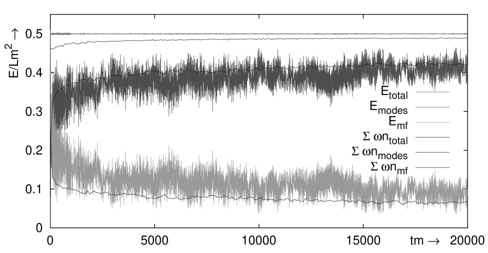
FIG. 5.: The total energy density $E/Lm^{2}$ (horizontal line at 0.5), energy density of the mean field (lower band) and of the modes (higher band). Also plotted are the various energy densities in the quasiparticle interpretation, $\sum_{k}n_{k}\omega_{k}/Lm^{2}$.

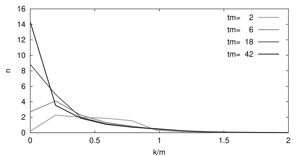
FIG. 6.: Particle number $n_{k}$ versus $k/m$ for early times.

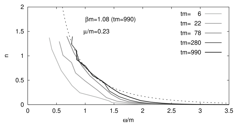
FIG. 7.: Particle number $n_{k}$ (modes only) versus $\omega_{k}$ for early times.

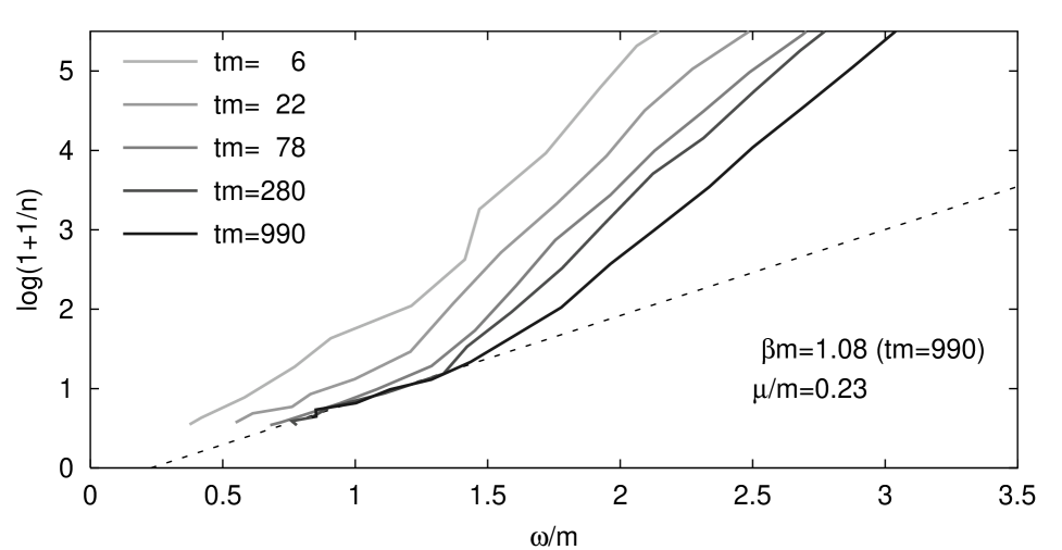
FIG. 8.: Particle number $\log(1+1/n_{k})$ (modes only) versus $\omega_{k}$ for early times. The straight line is a Bose-Einstein fit for the latest time, over $\omega/m<1.2$.

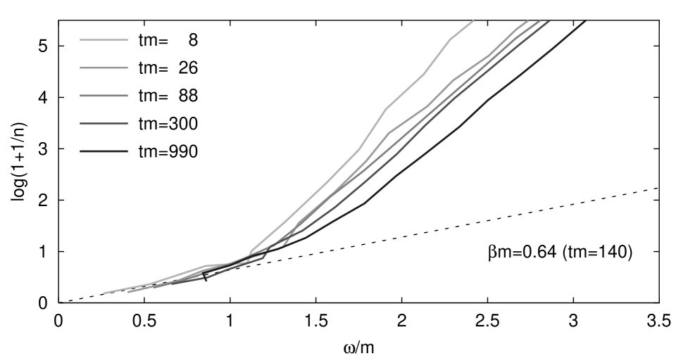
FIG. 9.: As in Fig. 8, including the mean field contribution.

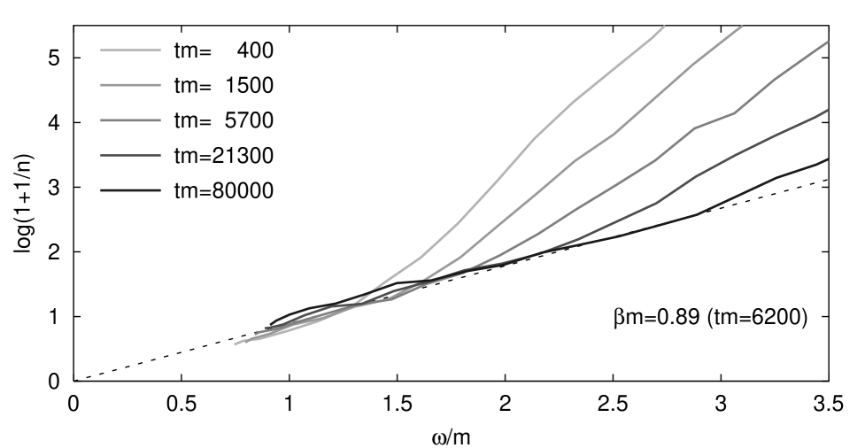
FIG. 10.: The particle numbers (modes only) for later times.

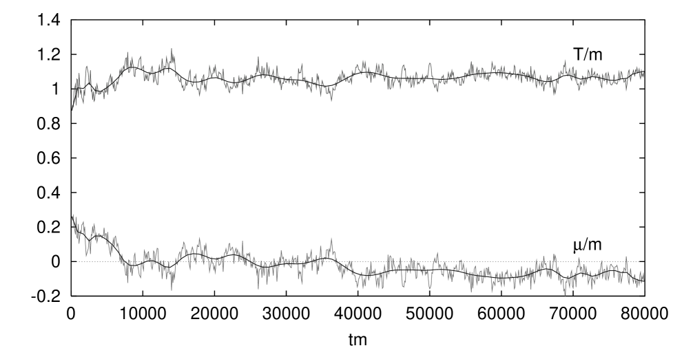
FIG. 11.: The Bose-Einstein temperature for particle numbers plotted in Fig. 10. The smoother lines are drawn to guide the eye.

FIG. 12.: Particle densities $n/m=\sum_{k}n_{k}/Lm$.

FIG. 13.: Energy distribution $n_{k}\omega_{k}/m$ (modes + mean field) for a small system with $N=16,Lm=1,E/Lm^{2}=36$.

FIG. 14.: Numerically computed auto-correlation functions $\log|F_{0\rm mf}(t)|$ versus time $tm_{T}$, with $m_{T}$ the temperature dependent mass. The coupling is weak, $\lambda/m_{T}^{2}=0.11$ and the temperature $T/m_{T}\approx 1.4$ for the smaller volume (with significant deviations from the Bose-Einstein distribution) and $\approx 1.6$ for the larger volume (reasonably BE).

REFERENCES

- [1] D. Bödeker, G.D. Moore, K. Rummukainen, Phys. Rev. D61 (2000) 056003, hep-ph/9907545.
- [2] W.H. Tang, J. Smit, Nucl. Phys. B540 (1999) 437, hep-lat/9805001.
- [3] S. Yu. Khlebnikov, I.I. Tkachev, Phys. Rev. Lett. 77 (1996) 219; T. Prokopec, T. Roos, Phys. Rev. D55 (1997) 3768, hep-ph/9610400; G. Felder, L. Kofman, Phys. Rev. 63 (2001) 103503, hep-ph/0011160.
- [4] J. García-Bellido, D.Y. Grigoriev, A. Kusenko, M. Shaposhnikov, Phys. Rev. D60 (1999) 123504, hep-ph/9902449. A. Rajantie, P.M. Saffin, E.J. Copeland, Nucl. Phys. B587 (200) 403, hep-ph/0012097.
- [5] G. Parisi, Europhys. Lett 40 (1997) 357;
- [6] G. Aarts, G.F. Bonini, Ch. Wetterich, Nucl. Phys. B587 (2000) 403, hep-ph/0003262.
- [7] G. Aarts, G.F. Bonini and Ch. Wetterich, Phys. Rev. D63 (2001) 025012, hep-ph/0007357.
- [8] G. Aarts, J. Smit, Phys. Rev. D61 (2000) 025002, hep-ph/9906538; Nucl. Phys. B555 (1999) 355, hep-ph/9812413.
- [9] G. Aarts, J. Smit, Nucl. Phys. B511 (1998) 451, hep-ph/9707342; Phys. Lett. B393 (1997) 395, hep-ph/9610415.
- [10] P. Arnold, Phys. Rev. D55 (1997) 7781, hep-ph/9701393;
- [11] B.-J. Nauta, Nucl. Phys. B575 (2000) 383, hep-ph/9906389; G. Aarts, B.-J. Nauta, Ch. G. van Weert, Phys. Rev. D61 (2000) 105002, hep-ph/9911463.
- [12] D. Boyanovsky, H.J. de Vega, astro-ph/0006446.
- [13] F. Cooper, Y. Kluger, E. Mottola, J.P. Paz, Phys. Rev. D51 (1995) 2377; M.A. Lampert, J. Dawson, F. Cooper, Phys.Rev. D54 (1996) 2213, hep-th/9603068.
- [14] B. Mihaila, F. Cooper and J.F. Dawson, Phys. Rev. D56 (1997) 5400, hep-ph/9705354.
- [15] B. Mihaila, T. Athan, F. Cooper, J. Dawson, S. Habib, Phys.Rev. D62 (2000) 125015, hep-ph/0003105.
- [16] A.V. Ryzhov and L.G. Yaffe, Phys. Rev. D62 (200) 125003, hep-ph/0006333.
- [17] B. Mihaila, F. Cooper and J.F. Dawson, Phys. Rev. D63 (2001) 046003, hep-ph/0006254.
- [18] J. Berges and J. Cox, hep-ph/0006160.
- [19] D. Boyanovsky, H. J. de Vega, R. Holman, J. F. J. Salgado, Phys. Rev. D54 (1996) 7570, hep-ph/9608205.
- [20] L. Mandel and E. Wolf, Optical coherence in quantum optics, (Cambridge University Press, Cambridge 1995); J.R. Klauder and B.-S. Skagerstam, Coherent States, World Scientific 1985.
- [21] H.-S. Roh, T. Matsui, Eur. Phys. J. A1 (1998) 205, nucl-th/9611050.
- [22] B.S. DeWitt, Dynamical theory of groups and fields, (Blackie 1965, in ‘Relativity, Groups and Topology’, Gordon and Breach 1964).
- [23] F. Cooper, S. Habib, Y. Kluger, E. Mottola, Phys. Rev. D55 (1997) 6471, hep-ph/9610345.
- [24] M. Sallé, J. Smit and J.C. Vink, hep-ph/0008122; Nucl. Phys. (Proc. Suppl.) 94 (2001) 427, hep-lat/0010054.
- [25] M. Sallé, J. Smit and J.C. Vink, hep-ph/0012362.