Nonlinear effects in Compton scattering at photon colliders

Abstract

The backward Compton scattering is a basic process at future higher energy photon colliders. To obtain a high probability of e$\to\gamma$ conversion the density of laser photons in the conversion region should be so high that simultaneous interaction of one electron with several laser photons is possible (nonlinear Compton effect). In this paper a detailed consideration of energy spectra, helicities of final photons and electrons in nonlinear backward Compton scattering of circularly polarized laser photons is given. Distributions of $\gamma\gamma$ luminosities with total helicities 0 and 2 are investigated. Very high intensity of laser wave leads to broadening of the energy (luminosity) spectra and shift to lower energies (invariant masses). Beside complicated exact formulae, approximate formulae for energy spectrum and polarization of backscattered photons are given for relatively small nonlinear parameter $\xi^{2}$ (first order correction). All this is necessary for optimization of the conversion region at photon colliders and study of physics processes where a sharp edge of the luminosity spectrum and monochromaticity of collisions are important.

PACS: 13.60.Fz; 13.88.+e; 42.60; 12.20.Ds

1 Introduction

The process of backward Compton scattering (BCS) is a basic process at Photon Linear Colliders (PLC), i.e. $\gamma$e and $\gamma\gamma$ colliding beams based on e⁺e^- (ee) linear colliders [1, 2, 3, 4, 5]. A detailed description of basic scheme of photon colliders and main characteristics of colliding $\gamma$e and $\gamma\gamma$ beams can be found in papers [2, 3]. In the latter non-trivial polarization effects in $\gamma$e and $\gamma\gamma$ interactions are also investigated. Further development of these ideas can be found elsewhere [6, 7, 8, 9, 10, 11, 12, 13, 14, 15, 16, 17, 18].

When a density of laser photons is very high, the processes in the conversion region can become nonlinear due to simultaneous interaction of electrons with several laser photons [19, 20, 21, 22]:

$$e(p)+n\gamma(k_{0})\to e(p^{\prime})+\gamma(k)\;,\;\;\quad n\geq 1\;,$$ (1)

$$\gamma(k)+s\gamma(k_{0})\to e^{+}(p_{+})+e^{-}(p_{-})\;,\;s\geq 1\;.$$ (2)

The first of these nonlinear processes (i.e. a process of nonlinear BCS) leads to widening energy spectra of scattered high energy photons and the second one lowers e⁺e^- pair production threshold [19, 20, 21, 22]. An interaction of electrons and positrons with an electromagnetic wave effectively increases the mass of the electron and this increase is characterized by an intensity parameter $\xi^{2}$:

$$m^{2}\rightarrow m^{2}_{\ast}=m^{2}\;(1+\xi^{2})\;,\;\xi^{2}=n_{\gamma}\left({4\pi\alpha\over m^{2}\omega_{0}}\right)\;=\;-{e^{2}\;a^{2}\over m^{2}}\;,$$ (3)

where $n_{\gamma}$ is the photon density in the wave, $\omega_{0}$ is the energy of the photons, $a$ is the amplitude of the a classical 4-potential of electromagnetic wave, $e$ and $m$ are the charge and the mass of the electron and $\alpha$ being the fine structure constant.  A systematic theoretical investigation of the nonlinear processes (1) and (2) has been done in papers [20, 21], and an experimental study has been carried out in papers [22].

At photon colliders one has “to convert” almost all electrons to high energy photons. To achieve this with minimum laser energy the laser light should be optimally focused, namely the length of the laser bunch and the Rayleigh length (the depth of the laser focus) should be approximately equal to the electron bunch length [2, 6, 7]. In this case the transverse size follows from the transverse emittance of the laser beam which is equal to $\lambda/4\pi$ (diffraction limit). It turns out that for beam parameters considered for photon colliders the parameter $\xi^{2}$ at optimum focusing may be larger than its acceptable value $\sim$0.2–0.3. To decrease $\xi^{2}$ (photon density) keeping conversion probability constant one has to make the photon bunch at the focal point longer and wider that requires larger laser flash energy. So, nonlinear effects in Compton scattering are very important for optimization of photon colliders (better quality of spectra needs larger flash energy).

In this paper we analyze in detail the influence of nonlinear effects on main characteristics of $\gamma$e and $\gamma\gamma$ collisions, namely, the energy spectra of photons, polarization of final photons and electrons, and the distribution of both the total spectral luminosity of $\gamma\gamma$ collisions and that for the total helicity 0 and 2. As we will see below the nonlinear effects are important. They must be taken into account at simulations of PLC. For comprehensive simulation of a PLC [7, 9, 11, 23] including processes multiple BCS one has to know not only the differential cross section of the reaction (1) but energy, angles and polarization of final photons and electrons.

2 The differential cross section for nonlinear BCS

In the case of head-on collision between ultrarelativistic electrons and photons of circularly polarized laser waves, the energy dependence of the differential cross section of process (1) as a function of $y=\omega/\varepsilon$ (where $\varepsilon$ is the electron energy) has the following form [23, 24, 25, 26, 27, 28]:

$${d\sigma_{c}\over dy}(\lambda,\lambda_{e},\lambda^{\prime},\lambda_{e}^{\prime}) = {\pi\alpha^{2}\over 2xm^{2}\xi^{2}}\sum_{n=1}^{\infty}\{\,(1+\lambda_{e}\lambda_{e}^{\prime})F_{1n}$$ (4)

$$+ \lambda(\lambda_{e}+\lambda_{e}^{\prime})F_{2n}+\lambda^{\prime}(\lambda F_{3n}+\lambda_{e}F_{4n})+\lambda_{e}\lambda_{e}^{\prime}F_{5n}\,\}\,,$$

$$F_{1n} = -4\;J_{n}^{2}+\xi^{2}\;\left(1-y+{1\over 1-y}\right)\;(J_{n-1}^{2}+J_{n+1}^{2}-2J_{n}^{2})\;,$$

$$F_{2n} = \xi^{2}\left(-1+y+{1\over 1-y}\right)\;\left(1-2{y\over y_{n}}{(1-y_{n})\over(1-y)}\right)\;(J_{n-1}^{2}-J_{n+1}^{2})\;,$$

$$F_{3n} = \xi^{2}\;\left(1-y+{1\over 1-y}\right)\;\left(1-2\;{y\over y_{n}}{(1-y_{n})\over(1-y)}\right)\;(J_{n-1}^{2}-J_{n+1}^{2})\;,$$ (5)

$$F_{4n} = -4y\;J_{n}^{2}+\xi^{2}\left(-1+y+{1\over 1-y}\right)\;(J_{n-1}^{2}+J_{n+1}^{2}-2J_{n}^{2}\;)\;,$$

$$F_{5n} = 4J_{n}^{2}\left(1+y-{1\over 1-y}\right)\;,\;\;$$

$$z_{n} = {2n\xi\over\sqrt{1+\xi^{2}}}\;\sqrt{\alpha_{n}}\,,\,\alpha_{n}=r_{n}(1-r_{n})={y\over y_{n}}\left(1-{y\over y_{n}}\right){(1-y_{n})\over(1-y)^{2}}\,,$$ (6)

$$y_{n} = {u_{n}\over 1+u_{n}}\,,\,r_{n}={y\over u_{n}(1-y)}\,,u_{n}={nx\over 1+\xi^{2}}\;,\;x={2k_{0}p\over m^{2}}\;={4\omega_{0}\varepsilon\over m^{2}}\;,\;$$ (7)

where $J_{n},J_{n\pm 1}$ are the various order Bessel functions of the same argument $z_{n}$ (6): $J_{n}=J_{n}(z_{n})$. Here the $y=\omega/\varepsilon$ changes in the range $0\leq y\leq y_{n}$. The expression, standing in front of the sum (4) gives the probability for the $n$-th harmonic to be radiated in the case when polarization states of both initial and final electrons and photons are $\lambda_{e}=\pm 1,\lambda_{e}^{\prime}=\pm 1,\lambda=\pm 1,\lambda^{\prime}=\pm 1$.

It should be noted that with backward scattering (when $y=y_{n}$), all the functions $F_{in}$ are zeroes at $n>1$. This means that only the first harmonic photons can be radiated in the direction along that of the initial electron beam. Higher harmonic photons can not be radiated in such conditions because of the helicity conservation of $e+n\gamma_{0}$ particles before and $e+\gamma$ after the interaction [25].

Using (4) one can obtain an expression for the degree of the longitudinal polarization of the final electron in the case when the final photon polarization is not detected:

$$\lambda_{e}^{f}=\sum_{n=1}^{\infty}\;(\lambda_{e}\;F_{1n}+\lambda_{e}\;F_{5n}+\lambda\;F_{2n})\;/\;\sum_{n=1}^{\infty}\;(\;F_{1n}+\lambda\lambda_{e}\;F_{2n}\;)\;.$$ (8)

Summing (4) over polarizations of the final electrons, one obtains the differential cross section taking into account the polarizations of three particles: [24, 25, 26, 27, 28]:

$${d\sigma_{c}\over dy}(\lambda,\lambda_{e},\lambda^{\prime})={\pi\alpha^{2}\over xm^{2}\xi^{2}}\sum_{n=1}^{\infty}(\;F_{1n}+\lambda\lambda_{e}F_{2n}+\lambda\lambda^{\prime}F_{3n}+\lambda_{e}\lambda^{\prime}F_{4n}\;)\;.$$ (9)

This formula allows one to find the degree of the circular polarization of the Compton photon $\lambda_{\gamma}^{f}$ for the case when the final electron polarization is not detected:

$$\lambda_{\gamma}^{f}=\sum_{n=1}^{\infty}\;(\lambda\;F_{3n}+\lambda_{e}\;F_{4n}\;)\;/\;\sum_{n=1}^{\infty}\;(\;F_{1n}+\lambda\lambda_{e}\;F_{2n}\;)\;.$$ (10)

After summation of (9) over polarizations of the final photons one gets the differential cross section of BCS in which polarizations of the initial particles are taken into account:

$${d\sigma_{c}\over dy}(\lambda,\lambda_{e})={2\pi\alpha^{2}\over xm^{2}\xi^{2}}\sum_{n=1}^{\infty}\;(\;F_{1n}+\lambda\lambda_{e}F_{2n}\;)\;.$$ (11)

The photon energy spectra $f(x,y)$ are defined through the differential cross section ${d\sigma_{c}}(\lambda,\lambda_{e})/dy$ (11) (for simplicity, we suppress below in all expressions the indexes $\lambda,\lambda_{e}$):

$$f(x,y)\equiv{1\over\sigma_{c}}\;{d\sigma_{c}\over dy}\,,\;\;\sigma_{c}={2\pi\alpha^{2}\over xm^{2}\xi^{2}}\sum_{n=1}^{n_{max}}\int_{0}^{y_{n}}(\;F_{1n}+\lambda\lambda_{e}F_{2n}\;)\,dy\;,$$ (12)

where $\sigma_{c}$ is the total cross section, $n_{max}\equiv n_{m}$ can be found in the condition that the series (11) converges. It defines the upper edge of the spectrum $y_{max}\equiv y_{m}=n_{m}x/(n_{m}x+1+\xi^{2})$ in the nonlinear BCS (see (7)).

In the case of hard $\gamma$ quanta colliding just after Compton conversion, the distribution of the spectral luminosity $\gamma\gamma$ collisions $L_{\mbox{$\gamma\gamma$}}$ over the invariant mass of colliding photons $W_{\mbox{$\gamma\gamma$}}=\sqrt{4\omega_{1}\omega_{2}},\,z=W_{\mbox{$\gamma\gamma$}}/2\varepsilon$ is expressed through the energy spectra of the photons (12):

$${1\over{L}_{\mbox{$\gamma\gamma$}}}{d{L}_{\mbox{$\gamma\gamma$}}\over dz}=2z\;\int_{-\eta_{m}}^{+\eta_{m}}f(x,ze^{+\eta})\;f(x,ze^{-\eta})\;d\eta\;,\;\;\eta\equiv\ln\sqrt{y_{1}/y_{2}}\;,$$ (13)

where $\eta$ is the rapidity of the $\gamma\gamma$ system, $y_{i}=\omega_{i}/\varepsilon$ are parts of energies which are taken by photons moving opposite directions 1 and 2. Here $z$ varies between 0 and $z_{m}=W_{m}/2\varepsilon=y_{m}$ with $W_{m}$ being the maximum value of the invariant mass of the colliding photons $W_{\mbox{$\gamma\gamma$}}$, $W_{m}=2\omega_{m}$, and $\eta$ lies in the region $|\eta|\leq\ln(y_{m}/z)$.

In the case of nonlinear BCS the photon scattering angle is unique function of the photon energy analogous in its form to that for linear Compton scattering:

$$\vartheta_{\gamma}^{n}(y)=\vartheta_{0}^{n}\sqrt{{y_{n}\over y}-1}\;,\;\vartheta_{0}^{n}={m_{\ast}\over\varepsilon}\,\sqrt{1+u_{n}}\,,\,m_{\ast}=m\sqrt{1+\xi^{2}}\,.$$ (14)

Below we analyze the influence of the nonlinear effect in BCS on the energy spectra of photons $f(x,y)$ (12), the helicities of the final photon $\lambda_{\gamma}^{f}$ (10) and electron $\lambda_{e}^{f}$ (8) as well as on the luminosity spectra of $\gamma\gamma$ collisions (13). Numerical calculations of these quantities will be carried out at the following values of the intensity parameter $\xi^{2}=0.0,0.3,1.0,3.0$ and for $x=4.8,20,50$. We will consider the three usual sets of the polarization stations of the colliding particles: (i) the initial electron is unpolarized ($\lambda_{e}=0$); ii) initial particles are completely polarized ($\lambda_{e}=1,\lambda=\pm 1$) and their spins are parallel ($\lambda\lambda_{e}=-1$); iii) the same for antiparallel spins ($\lambda\lambda_{e}=1$) (15)). In addition we will also study the case when the electron is not completely polarized $\lambda_{e}=0.8$ (16):

$$1)\to\lambda_{e}=0,\;\lambda = 1;\;2)\to\lambda_{e}=1,\;\lambda=-1;\;3)\to\lambda_{e}=1\;,\;\lambda=1\,,$$ (15)

$$2r) \to \lambda_{e}=0.8,\;\lambda=-1;\;3r)\to\lambda_{e}=0.8\;,\;\lambda=1\,,$$ (16)

As a rule, BCS is considered only in the region $2.5<x<4.8$. At $x>4.8$ in the conversion region a process of e⁺e^- pairs production becomes possible at collisions of Compton photons with photons of the same laser wave [2, 6]. The reaction threshold at $\xi^{2}=0$ is equal to $\omega_{m}\omega_{0}>m^{2}$, i.e. $x=2(1+\sqrt{2})\approx 4.828$. Above this threshold ($x\sim 8-20$) the cross section of the pair production is 1.5–5 times larger than that of BCS. This leads to knocking out the Compton photons and lowering the conversion coefficient [6, 7]. Nevertheless, we will also consider the region of higher $x$ being of interest for the experiments in which the maximum monochromatization of $\gamma\gamma$ collisions is required.

3 Energy spectra of photons

Results of numerical calculations of energy spectra of photons are shown in Fig.1. It is seen in Fig.1 that the energy spectra of photons depend strongly on the values of $\lambda\lambda_{e}$, $x$ and $\xi^{2}$. In the linear case at $x=4.8$ when spins of colliding electrons and photons of the laser wave are parallel ($\lambda\lambda_{e}=-1$), the number of high energy photons is almost two times larger than that for the unpolarized case (see Fig.1a). At $x=50$ the yield of hard photons increases by a factor of three (see Fig.1i). So, simultaneously with increasing $x$ (i.e. with increasing $\omega_{0}$ or $\varepsilon$) there exits an effective “pumping” soft photons into hard ones. This leads to noticeable improving the monochromaticity of $\gamma\gamma$ collisions. In contrast, if spins of electrons and laser photons are antiparallel ($\lambda\lambda_{e}=+1$) the number of hard photons decreases (cf. curves 1 and 3 in Fig.1(a,e,i)). Accordingly, the monochromaticity of collisions goes down.

Nonlinear effects in BCS ($\xi^{2}\neq 0$) lead to significant changes in energy spectra in comparison with those in the linear BCS ($\xi^{2}=0$). First, simultaneous absorption of a few photons from a laser wave induces widening spectra of hard $\gamma$ quanta and a generation of additional peaks corresponding to radiation of higher harmonics. This widening at the same parameter $x$ is more pronounced the higher the intensity of the wave (cf. Fig.1(a-d), (e-h), (i-l)). A consequence of the widening is the decrease of the height of the peak for the first harmonics in comparison with that in the linear case. This is clearly seen if one compares Figs.1(a-d) and so on.

Second, due to increase of the electron effective mass (3) the scattered photon have lower energies, i.e. the first harmonic is shifted to lower values of $y$ (see Fig.1(a-d) and so on). With increasing the parameter $x$ the relative shift of the first harmonic decreases [25, 7].

At a relatively small intensity of the laser wave ($\xi^{2}\sim 0.3$) the main contribution give photons of the first harmonic and the probability for generation of higher harmonics is small (see Fig.1(b,f,j)). At $\xi\sim 1$ the widening the spectra because of nonlinear effects is accompanied by an increase of the yield of photons with energies higher than the maximum energy of the first harmonic (see. Fig.1(c,g,k)). At last, at high intensities ($\xi^{2}\geq 1$) the nonlinear processes of scattering on many photon can become comparable with one photon scattering (see Fig.1d) and even predominant (at $\xi^{2}\gg 1$) [21, 25].

4 Polarization of final photons

Results of numerical calculations for the energy dependence of the degree of the circular polarization of Compton photons (10) are given in Fig.2. We begin our consideration with the case of $\xi^{2}=0$ and $\lambda\lambda_{e}=1$ (the case of bad monochromaticity). It is seen in Fig.2(e,i), that at $x=20,50$ the helicity of the Compton photon is practically constant and equal to one in all energy range $0<y<y_{m}$. As a result, the contribution of the state of the $\gamma\gamma$ system with the spin 2 in the distribution of the total spectral luminosity of $\gamma\gamma$ collisions will be almost equal to zero. Note that the increase of the intensity parameter $\xi^{2}$ up to 1 at $x=50$ does not lead to noticeable changes in such a character of the behavior of $\lambda_{\gamma}^{f}$. At the same time, by going to the realistic electron polarizations ($\lambda_{e}=0.8$) the behavior of the helicity of Compton photons (see Fig.2(i-l)) becomes more pronounced.

When the monochromaticity is best ($\lambda\lambda_{e}=-1$), both at $\xi^{2}=0$ and $\xi^{2}\neq 0$ there exists a rather wide energy interval near $y\sim y_{m}$ where the scattered photons have a high degree of the polarizations (almost 100 %). If the initial electron polarization is less than 100 % and $\lambda=1$, the energy range of the high helicity becomes markedly narrower. High energy photons can have a high degree of circular polarization near $y\sim y_{m}$ at $\lambda=1$ even if the initial electron is unpolarized ($\lambda_{e}=0$).

Nonlinear effects induce additional peaks in the energy dependence of the helicity of the Compton photons. The height of the first peak which corresponds to the radiation of the first harmonic decreases in magnitude in comparison with the case of liner BCS and moves to lower energies. It is worth mentioning that at small $y$ the helicity $\lambda_{\gamma}^{f}$ of the scattered photons is practically independent of the electron polarization $\lambda_{e}$.

5 Polarization of the final electrons

Our results for the dependence of the degree of longitudinal polarization of the scattered electron (8) on its energy $\varepsilon^{\prime}/\varepsilon=1-y$ are shown in Fig.3. It is seen in Fig.3a for $x=4.8$ and $\xi^{2}=0$ that an unpolarized electron being scattered from a totally polarized laser beam can acquire high a degree of longitudinal polarization (94 %) in the region of minimal values of the energy $\varepsilon^{\prime}$. This is in agreement with the result of a paper [29]. In the case of linear BCS at $x=20,50$ the degree of the polarization of the final electron can reach almost 100 % (see Fig.3(e,i)).

Because of nonlinear effects, instead of one peak seen in Fig.3(a,e,i) there emerge a few (for example, three at $\xi^{2}=0.3$). The height of the first peak corresponding to the first harmonic decreases in magnitude in comparison with the case of linear BCS and moves to higher energies. At higher intensities of the wave when $\xi^{2}=1.0,3.0$ (see Fig. 3(c,d,g,h,k,l)) one has rather complicate a behavior due to the absorption of many photons.

6 Distribution of total spectral luminosity of $\gamma\gamma$ collisions

The total spectral luminosity of $\gamma\gamma$ collisions (13) are shown in Fig.4. The luminosity spectra in Fig.4(a,e,i) and the energy spectra in Fig.1(a,e,i) are consistent with each other. It should be noted that in the approximation when the intensity of the laser wave can be neglected, the distributions of the spectral luminosity over the invariant mass have a sharp edge at $z=z_{m}$. This can be very important in the search of the Higgs boson [16].

It is seen in Fig.4 that the behavior of the spectral luminosities is analogous to that of photon energy spectra. Together with increasing the wave intensity we observe the raising of the luminosity in the region of low and intermediate invariant masses of colliding photons, and the decreasing of the height of the peaks. There emerges a long “tail” in the range of high invariant masses. Widening the luminosity distribution in comparison with linear BCS leads to the appearance of small “triangles” located on the right side of the edge of the spectrum $\xi^{2}=0$. The slope of the curves for the luminosity with respect to the abscissa axis essentially changes. As a result, the sharp edge of the spectral luminosity, which is inherent in linear BCS, disappears which leads to noticeable decrease of the monochromaticity of $\gamma\gamma$ collisions. All unfavorable moments due to nonlinear effects are less important when the parameter $x$ increases. This is clearly seen in Fig.4 for to $x=4.8$,$x=20$ and $x=50$.

7 The distribution of spectral luminosities for a $\gamma\gamma$ system with spins 0 and 2.

The spectral luminosity of $\gamma\gamma$ collisions in the case of spins 0 and 2 of the $\gamma\gamma$ system, $dL_{0}/dz$ and $dL_{2}/dz$, are shown in Fig.5 (for $\lambda\lambda_{e}=0,\pm 1$) and Fig.6 (for $\lambda\lambda_{e}=\pm 0.8$). Our calculations for linear BCS at $\lambda\lambda_{e}=-1$ show that near the peak, i.e. for $0.9z_{m}\leq z\leq z_{m}$, the main contribution to the total luminosity stems from the state with the spin 0 (see Fig.5(b,e,h)). It was noted in papers [7, 11], that the smallness the ratio $dL_{2}/dL_{0}$ at $x=4.8$ in the peak region can be very important in search of the Higgs boson. If the electron polarization is less 100 % ($\lambda\lambda_{e}=-0.8$) then the contribution of the spin 2 states grows.

For $\lambda\lambda_{e}=1$ and $\xi^{2}=0$ the ratio $dL_{2}/dL_{0}$ is also small but in the full region $0\leq z\leq z_{m}$ for all $x$ (see Fig.5(c,f,i)). One can see also that with increasing $x$ the contribution of the spin 2 state in the total luminosity is decreasing. It can be explained by the fact that at high $x$ and $\lambda\lambda_{e}=1$ the scattered photon is almost totally polarized (see Fig.2(e,i) and the discussion above). At a collision of two such photons moving in reverse directions, only the total spin 0 system is possible. Since in the case under consideration nonlinear effects have small influence on the polarization of final photons the suppression above will take place at high intensities too (see Fig.5(f,i)). Contribution of the spin 2 state significantly increase when the electron polarization $\lambda_{e}\ <1$ (see Fig.6(b,d,f)).

8 Conclusion

The process of backward Compton scattering is the best method for obtaining high energy photons at future photon colliders. The the required density of laser photons in the conversion region is so high that nonlinear effects in the Compton scattering take place. The lead to some increase of the maximum energy of scattered photons, however, when the intensity of the laser wave grows the monochromaticity of $\gamma\gamma$ collisions becomes worse and the spectral luminosity is shifted to the region of low and intermediate invariant masses and less photons remain in the high energy peak. This is due the fact that only photons of the first harmonic can be emitted along the direction of the initial electron beam and produce photons near kinematical limit. Such a behavior is not permitted for photons of higher order harmonics because of the helicity conservation for the particle system $e+n\gamma_{0}$ before interaction and $e+\gamma$ after interaction [25]. This leads to widening of the angular distribution of the higher order harmonics and in turn decreases the monochromaticity of $\gamma\gamma$ collisions.

In this paper formulae for energy distributions of final photons end electrons and their polarizations are given in the case of nonlinear Compton scattering. Numerous figures for energy spectra and luminosity distributions at different values of initial beam polarizations and parameters $x$ and $\xi^{2}$ are presented, which allows to see main tendencies.

9 Appendix

In the present paper the numerical calculations of energy spectra, polarizations of final electrons and photons and luminosities are carried out making the use of precise formulae for the corresponding differential cross sections. However, for small intensities when $\xi^{2}\ll 1$ one can restrict oneself to the contribution of two first harmonics to the differential cross sections (4), (9), and (11) and obtain for them approximate expressions. To this end, it is quite enough to expand the Bessel functions in (4) in terms of the parameter $\Delta=\xi^{2}/(1+\xi^{2})$ (rather than in terms of $\xi^{2}$ as is done in [20]) and for $u_{n}\,(y_{n})$ (7) to use exact formulae. Only in this way can one reveal the above pointed out kinematical features of the functions (5) $F_{in}\,(i=1,\ldots 5)$. As a result, we have (see [25]):

$${F_{11}\over\xi^{2}} = 1-y+{1\over 1-y}-4\alpha_{1}-4\alpha_{1}\Delta\;\Bigg{(}-y+{1\over 1-y}-\alpha_{1}\Bigg{)},$$

$${F_{21}\over\xi^{2}} = \Bigg{(}-1+y+{1\over 1-y}\Bigg{)}\Bigg{(}1-2{y\over y_{1}}{(1-y_{1})\over(1-y)}\Bigg{)}\big{(}1-2\alpha_{1}\,\Delta\big{)}\;,$$

$${F_{31}\over\xi^{2}} = \Bigg{(}1-y+{1\over 1-y}\Bigg{)}\Bigg{(}1-2{y\over y_{1}}{(1-y_{1})\over(1-y)}\Bigg{)}\big{(}1-2\alpha_{1}\,\Delta\big{)}\;,$$ (17)

$${F_{41}\over\xi^{2}} = -1+y+{1\over 1-y}-4\alpha_{1}\,y-4\alpha_{1}\Delta\,y\Bigg{(}-\alpha_{1}+{1\over 1-y}\Bigg{)},$$

$${F_{51}\over\xi^{2}} = 4\alpha_{1}(1-\Delta(1+\alpha_{1}))\,\Bigg{(}1+y-{1\over 1-y}\Bigg{)}\,,$$

for the first harmonic;

$${F_{12}\over\xi^{2}} = 4\alpha_{2}\Delta\,\Bigg{(}1-y+{1\over 1-y}-4\alpha_{2}\Bigg{)},$$

$${F_{22}\over\xi^{2}} = 4\alpha_{2}\Delta\,\Bigg{(}-1+y+{1\over 1-y}\Bigg{)}\Bigg{(}1-2{y\over y_{2}}{(1-y_{2})\over(1-y)}\Bigg{)},$$

$${F_{32}\over\xi^{2}} = 4\alpha_{2}\Delta\,\Bigg{(}1-y+{1\over 1-y}\Bigg{)}\Bigg{(}1-2{y\over y_{2}}{(1-y_{2})\over(1-y)}\Bigg{)},$$ (18)

$${F_{42}\over\xi^{2}} = 4\alpha_{2}\Delta\,\Bigg{(}-1+y+{1\over 1-y}-4\alpha_{2}y\Bigg{)},$$

$${F_{52}\over\xi^{2}} = 16\alpha_{2}^{2}\Delta\,\Bigg{(}1+y-{1\over 1-y}\Bigg{)}\,,$$

for the second harmonic.

The total cross section of the process (1) $\sigma_{c}(\lambda,\lambda_{e})$ (12) has the following form [25]:

$$\sigma_{c}(\lambda,\lambda_{e})={2\pi\alpha^{2}\over xm^{2}}\;(\;f_{1}+\lambda\lambda_{e}\,f_{2}\,)\,,\,f_{1}=f_{11}+f_{12}\,,f_{2}=f_{21}+f_{22}\,,$$ (19)

where

$$f_{11} = \Bigg{(}1-{4\over u_{1}}-{8\over u_{1}^{2}}\Bigg{)}\ln(1+u_{1})+{1\over 2}+{8\over u_{1}}-{1\over 2(1+u_{1})^{2}}-\Delta\Bigg{(}2+{44\over 3u_{1}}-$$

$$- {16\over u_{1}^{2}}-{16\over u_{1}^{3}}-{2\over 1+u_{1}}-{8\over u_{1}}\Bigg{(}1+{1\over u_{1}}-{3\over u_{1}^{2}}-{2\over u_{1}^{3}}\Bigg{)}\ln(1+u_{1})\Bigg{)}\,,$$

$$f_{21} = \Bigg{(}1+{2\over u_{1}}\Bigg{)}\ln(1+u_{1})-{5\over 2}+{1\over 1+u_{1}}-{1\over 2(1+u_{1})^{2}}-$$ (20)

$$- \Delta\Bigg{(}{1\over 3}+{4\over u_{1}}-{8\over u_{1}^{2}}-{1\over 1+u_{1}}-{2\over u_{1}}\Bigg{(}1-{4\over u_{1}^{2}}\Bigg{)}\ln(1+u_{1})\Bigg{)}\,,$$

$$f_{12} = 4\Delta\Bigg{(}{1\over 2}+{2\over 3u_{2}}-{16\over u_{2}^{2}}-{16\over u_{2}^{3}}-{1\over 2(1+u_{2})}-$$

$$- {1\over u_{2}}\Bigg{(}1-{6\over u_{2}}-{24\over u_{2}^{2}}-{16\over u_{2}^{3}}\Bigg{)}\ln(1+u_{2})\Bigg{)}\,,$$

$$f_{22} = 4\Delta\Bigg{(}{1\over 6}+{2\over u_{2}}-{4\over u_{2}^{2}}-{1\over 2(1+u_{2})}-{1\over u_{2}}\Bigg{(}1-{4\over u_{2}^{2}}\Bigg{)}\ln(1+u_{2})\Bigg{)}\,.$$

Note that computations of the energy spectra of photons for $x=4.8$ and $\xi^{2}=0.3$ done with the use either of exact formulae (12) or approximated ones (17), (18) and (19) lead to practically the same results. For example, the difference in the magnitude of peaks corresponding to first harmonics is only about 0.5 %.

Figure Caption

Fig.1 The energy spectra of Compton photons (12) for various values of $x$, $\xi^{2}$ and $\lambda\lambda_{e}$. In Fig.(a-d), (e-h), and (i-l) parameter $x=4.8,20$, and $50$, respectively. In Fig.(a,e,i), (b,f,j), (c,g,k), and (d,h,l) the intensity parameter $\xi^{2}=0.0,0.3,1.0$, and $3.0$, respectively. Lines labelled by 1, 2, 3 correspond to the choice of polarization stations of initial particles $\lambda_{e}=0,\lambda=1$; $\lambda_{e}=1,\lambda=-1$; $\lambda_{e}=1,\lambda=1$.

Fig.2 The energy dependence of the helicity of Compton photons (10) for various values of $x$, $\xi^{2}$ and $\lambda\lambda_{e}$. In Fig.(a-d), (e-h), and (i-l) parameter $x=4.8,20$, and $50$, respectively. In Fig.(a,e,i), (b,f,j), (c,g,k), and (d,h,l) the intensity parameter $\xi^{2}=0.0,0.3,1.0$, and $3.0$, respectively. The full, long-dash-dotted, and dashed curves correspond to the set of polarization states $\lambda_{e}=0,\lambda=1$; $\lambda_{e}=1,\lambda=-1$; $\lambda_{e}=1,\lambda=1$, respectively. Short-dash-dotted and dotted curves correspond to choice $\lambda_{e}=0.8,\lambda=-1$ and $\lambda_{e}=0.8,\lambda=+1$, respectively.

Fig.3 The degree of the longitudinal polarization of final electron (8) as a function of its energy $\varepsilon^{\prime}/\varepsilon=1-y$ for various values $x$, $\xi^{2}$, and $\lambda\lambda_{e}$. In Fig.(a-d), (e-h), and (i-l) the parameter $x=4.8,20$ and $50$, respectively. In Fig.(a,e,i), (b,f,j), (c,g,k), and (d,h,l) the intensity parameter $\xi^{2}=0.0,0.3,1.0$, and $3.0$, respectively. In Fig.(a-l) the solid, dotted, and dashed curves correspond to $\lambda_{e}=0,\lambda=1$; $\lambda_{e}=1,\lambda=-1$; $\lambda_{e}=1,\lambda=1$, respectively.

Fig.4 The distribution of total spectral luminosity of $\gamma\gamma$ collisions (13) over the invariant mass of photons $z=W_{\mbox{$\gamma\gamma$}}/2\varepsilon$. In Fig.(a-d), (e-h), and (i-l) parameter $x=4.8$, 20, and 50, respectively. In Fig.(a,e,i), the intensity parameter $\xi^{2}=0.0$, and the curves 1, 2, and 3 stand for the choice of the polarizations $\lambda_{e}=0,\lambda=1$; $\lambda_{e}=1,\lambda=-1$; $\lambda_{e}=1,\lambda=1$. The curves in Fig.(b,f,j), (c,g,k), and (d,h,l) correspond to $\lambda\lambda_{e}=0$, $\lambda\lambda_{e}=-1$, and $\lambda\lambda_{e}=1$, respectively. In all these figures except for (a,e,i) the solid, dotted, dashed, and dash-dotted curves stand for the intensity parameter $\xi^{2}$ equal to 0.0, 0.3, 1.0, and 3.0, respectively.

Fig.5 The distribution of spectral luminosities $dL_{0}/dz$ and $dL_{2}/dz$ of the $\gamma\gamma$ system over the invariant mass of photons $z=W_{\mbox{$\gamma\gamma$}}/2\varepsilon$. Corresponding curves are labelled by numbers 0 and 2 (for spin 0 and 2). The left, central, and right panels correspond to $x=4.8$, 20, and 50, respectively. Fig.(a,d,g), (b,e,h), and (c,f,i) were built for $\lambda\lambda_{e}=0$, $\lambda\lambda_{e}=-1$, and $\lambda\lambda_{e}=1$, respectively. The solid, dotted, dashed, and dash-dotted curves correspond to the intensity parameter $\xi^{2}=0.0,0.3,1.0$, and $3.0$, respectively.

Fig.6 The distribution of spectral luminosities $dL_{0}/dz$ and $dL_{2}/dz$ of the $\gamma\gamma$ system over $z=W_{\mbox{$\gamma\gamma$}}/2\varepsilon$. Corresponding curves are labelled by numbers 0 and 2. The left, central, and right panels correspond to $x=4.8$, 20 and 50, respectively. Fig.(a,c,e) and (b,d,f) stand for $\lambda\lambda_{e}=-0.8$ and $\lambda\lambda_{e}=+0.8$, respectively. The solid, dotted, dashed, and dash-dotted curves correspond to the intensity parameter $\xi^{2}=0.0,0.3,1.0$, and $3.0$, respectively.

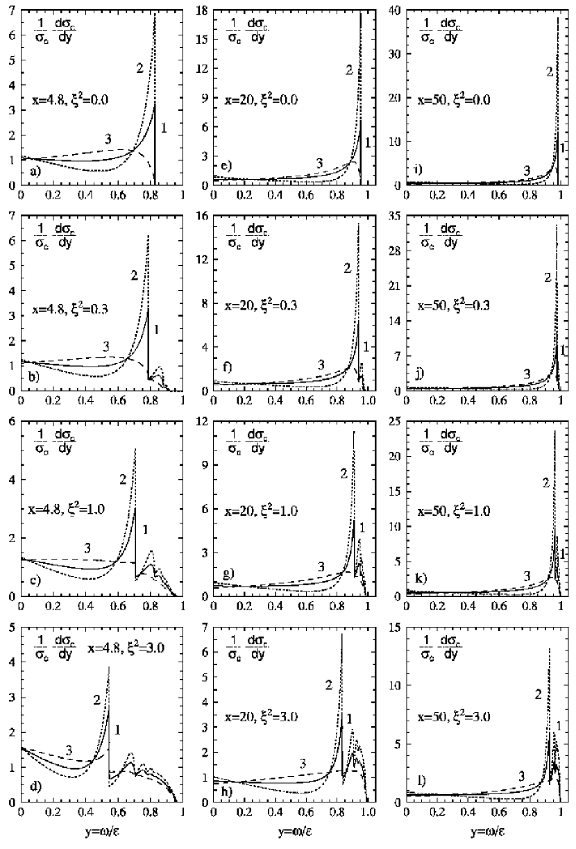
Figure 1: The energy spectra of Compton photons (12) for various values of $x$, $\xi^{2}$ and $\lambda\lambda_{e}$. In Fig.(a-d), (e-h), and (i-l) parameter $x=4.8,20$, and $50$, respectively. In Fig.(a,e,i), (b,f,j), (c,g,k), and (d,h,l) the intensity parameter $\xi^{2}=0.0,0.3,1.0$, and $3.0$, respectively. Lines labelled by 1, 2, 3 correspond to the choice of polarization stations of initial particles $\lambda_{e}=0,\lambda=1$; $\lambda_{e}=1,\lambda=-1$; $\lambda_{e}=1,\lambda=1$.

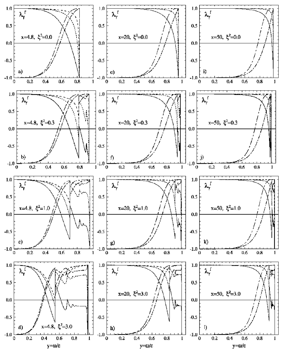
Figure 2: The energy dependence of the helicity of Compton photons (10) for various values of $x$, $\xi^{2}$ and $\lambda\lambda_{e}$. In Fig.(a-d), (e-h), and (i-l) parameter $x=4.8,20$, and $50$, respectively. In Fig.(a,e,i), (b,f,j), (c,g,k), and (d,h,l) the intensity parameter $\xi^{2}=0.0,0.3,1.0$, and $3.0$, respectively. The full, long-dash-dotted, and dashed curves correspond to the set of polarization states $\lambda_{e}=0,\lambda=1$; $\lambda_{e}=1,\lambda=-1$; $\lambda_{e}=1,\lambda=1$, respectively. Short-dash-dotted and dotted curves correspond to choice $\lambda_{e}=0.8,\lambda=-1$ and $\lambda_{e}=0.8,\lambda=+1$, respectively.

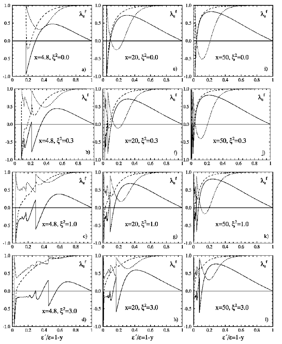
Figure 3: The degree of the longitudinal polarization of final electron (8) as a function of its energy $\varepsilon^{\prime}/\varepsilon=1-y$ for various values $x$, $\xi^{2}$, and $\lambda\lambda_{e}$. In Fig.(a-d), (e-h), and (i-l) the parameter $x=4.8,20$ and $50$, respectively. In Fig.(a,e,i), (b,f,j), (c,g,k), and (d,h,l) the intensity parameter $\xi^{2}=0.0,0.3,1.0$, and $3.0$, respectively. In Fig.(a-l) the solid, dotted, and dashed curves correspond to $\lambda_{e}=0,\lambda=1$; $\lambda_{e}=1,\lambda=-1$; $\lambda_{e}=1,\lambda=1$, respectively.

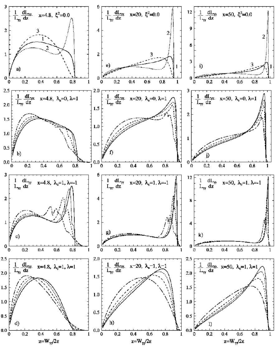
Figure 4: The distribution of total spectral luminosity of $\gamma\gamma$ collisions (13) over the invariant mass of photons $z=W_{\mbox{$\gamma\gamma$}}/2\varepsilon$. In Fig.(a-d), (e-h), and (i-l) parameter $x=4.8$, 20, and 50, respectively. In Fig.(a,e,i), the intensity parameter $\xi^{2}=0.0$, and the curves 1, 2, and 3 stand for the choice of the polarizations $\lambda_{e}=0,\lambda=1$; $\lambda_{e}=1,\lambda=-1$; $\lambda_{e}=1,\lambda=1$. The curves in Fig.(b,f,j), (c,g,k), and (d,h,l) correspond to $\lambda\lambda_{e}=0$, $\lambda\lambda_{e}=-1$, and $\lambda\lambda_{e}=1$, respectively. In all these figures except for (a,e,i) the solid, dotted, dashed, and dash-dotted curves stand for the intensity parameter $\xi^{2}$ equal to 0.0, 0.3, 1.0, and 3.0, respectively.

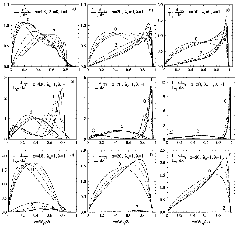
Figure 5: The distribution of spectral luminosities $dL_{0}/dz$ and $dL_{2}/dz$ of the $\gamma\gamma$ system over the invariant mass of photons $z=W_{\mbox{$\gamma\gamma$}}/2\varepsilon$. Corresponding curves are labelled by numbers 0 and 2 (for spin 0 and 2). The left, central, and right panels correspond to $x=4.8$, 20, and 50, respectively. Fig.(a,d,g), (b,e,h), and (c,f,i) were built for $\lambda\lambda_{e}=0$, $\lambda\lambda_{e}=-1$, and $\lambda\lambda_{e}=1$, respectively. The solid, dotted, dashed, and dash-dotted curves correspond to the intensity parameter $\xi^{2}=0.0,0.3,1.0$, and $3.0$, respectively.

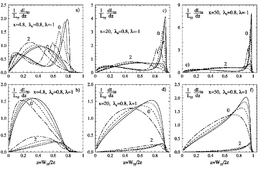
Figure 6: The distribution of spectral luminosities $dL_{0}/dz$ and $dL_{2}/dz$ of the $\gamma\gamma$ system over $z=W_{\mbox{$\gamma\gamma$}}/2\varepsilon$. Corresponding curves are labelled by numbers 0 and 2. The left, central, and right panels correspond to $x=4.8$, 20 and 50, respectively. Fig.(a,c,e) and (b,d,f) stand for $\lambda\lambda_{e}=-0.8$ and $\lambda\lambda_{e}=+0.8$, respectively. The solid, dotted, dashed, and dash-dotted curves correspond to the intensity parameter $\xi^{2}=0.0,0.3,1.0$, and $3.0$, respectively.

References

- [1] I. Ginzburg, G. Kotkin, V. Serbo, V. Telnov, Pizma ZhETF, 34 (1981) 514; JETP Lett. 34 (1982) 491; (Prep. INF 81-50, Novosibirsk, Feb.1981)
- [2] I. Ginzburg, G. Kotkin, V. Serbo, V. Telnov, Prep. INF 81-102, Novosibirsk, 1981; Prep. INF 81-92, Novosibirsk, Aug. 1981; Yad. Fiz 38 (1983) 372; Nucl. Instr. Meth. 205 (1983) 47.
- [3] I. Ginzburg, G. Kotkin, S. Panfil, V. Serbo, V. Telnov, Nucl.Instr. Meth. 219 (1984) 5; Prep. INF 81-160, Novosibirsk, 1982;
- [4] I. Ginzburg, G. Kotkin, S. Panfil, V. Serbo, Yad.Fiz. 38 (1983) 1021.
- [5] C. Akerlof, Preprint UMHE 81-59, Univ.of Michigan, 1981.
- [6] V. Telnov, Nucl.Instr.Meth., A294 (1990) 72.
- [7] V. Telnov, Nucl.Instr.Meth., A355 (1995) 3.
- [8] V. Telnov, Proc.of Intern.Vavilov’s Conference on nonlinear optics, Novosibirsk, June 24-26, 1997; Prep.Budker INP 97-71, Novosibirsk, 1997; eprint: hep-physics/9710014.
- [9] V. Telnov, Proc.of ITP Symp.on Future High Energy Colliders, Santa Barbara, USA, Oct. 21–25, 1996; AIP Conf.Proc., No 397, ed.Z.Parza, (AIP.New York 1997), p.259-273; Prep.Budker INP, 97-47, eprint: hep-physics/9706003.
- [10] V. Telnov, SLAC-PUB 7337 (1996), Prep.Budker INP 96-78 (1996), eprint: hep-ex/9610008; Phys.Rev.Lett. 78 (1997) 4757; erratum ibid 80 (1998) 2747.
- [11] D. Borden, D. Bauer and D. Caldwell, Phys.Rev., D48 (1993) 4018; SLAC-PUB 5715, UCSD-HEP 92-01.
- [12] Proc.of Workshop on Colliders, Berkeley CA, USA, 1994, Nucl. Instr.Meth., A355 (1995) 1.
- [13] Zeroth-Order Design Report for the Next Linear Collider LBNL-PUB-5424, SLAC Report 474, May 1996.
- [14] Conceptual Design of a 500 GeV Electron Positron Linear Collider with Integrated X-Ray Laser Facility DESY 97-048, ECFA-97-182. R.Brinkmann et al., Nucl. Instr. &Meth. A 406 (1998) 13.
- [15] JLC Design Study, KEK-REP-97-1, April 1997; I.Watanabe et. al.,KEK Report 97-17.
- [16] V. Telnov, Proc.of 2 nd Inter.Workshop on inter.at TeV energies, Santa Cruz, USA, Sept. 22-24, 1997; Int.J.Mod.Phys. A13 (1998) 2399; eprint: hep-ex/9802003.
- [17] V. Telnov, Proc. of the International Conference on the Structure and Interactions of the Photon (Photon 99), Freiburg, Germany, 23-27 May 1999, Nucl. Phys. Proc. Suppl. B82 (2000) 359; e-print: hep-ex/9908005.
- [18] V. Telnov, Photon collider at TESLA, these proceedings, e-print: hep-ex/0010033.
- [19] I. Ginzburg, G. Kotkin, S. Polityko, Yad.Fiz., 37 (1983) 368; Yad.Fiz. 40 (1984) 1495.
- [20] A. Nikishov, V. Ritus, Zh.Eksp.Teor.Fiz., 46 (1964) 776; Zh.Eksp.Teor.Fiz., 46 (1964) 1768; Zh.Eksp.Teor.Fiz. 47 (1964) 1130; Zh.Eksp.Teor.Fiz., 52 (1967) 1707; N. Narozhnyi, A. Nikishov, V. Ritus, Zh.Eksp.Teor.Fiz., 47 (1964) 931.
- [21] A. Nikishov, V. Ritus, Trudy FIAN, 111 (1979) (Proc. Lebedev Institute, in russian).
- [22] C. Bula, K. McDonald et al., Phys.Rev.Lett., 76 (1996) 3116, Phys.Rev.Lett., 79 (1997) 1626; Phys.Rev., D60 (1999) 092004.
- [23] K. Yokoya, CAIN2e, Code simulation for JLC, Users Manual.
- [24] Y. Grinchishin, M. Rekalo, Zh.Eksp.Teor.Fiz., 84 (1983) 1605.
- [25] M. Galynskii, S. Sikach, Sov.Phys.JETP, 101 (1992) 441.
- [26] Yu.S. Tsai, Phys.Rev., D48 (1993) 96.
- [27] E. Kuraev, M. Galynskii, M. Levchuk, Fiz.Elem.Chast.At.Yad., 31 (2000) 155.
- [28] M. Galynskii, S. Sikach, Fiz.Elem.Chast.Atom.Yadra, 29 (1998) 1133; eprint: hep-ph/9910284.
- [29] G. Kotkin, S. Polityko, V. Serbo, Yad.Fiz., 59 (1996) 2229; Nucl.Instr.Meth., A405 (1998) 30.