CERN-TH/2000-385

Neutrino Masses and Lepton-Flavor Violation in Supersymmetric Models
with lopsided Froggatt–Nielsen charges

Joe Sato^a and Kazuhiro Tobe^b

(a) Research Center for Higher Education, Kyushu University,
Ropponmatsu, Chuo-ku, Fukuoka, 810-8560, Japan

(b) CERN, Theory Division, CH-1211 Geneva 23, Switzerland

1 Introduction

One of big mysteries in the Standard Model (SM) of elementary particles is a problem of fermion masses. Since Yukawa couplings, which determine the magnitude of fermion masses, are totally free parameters in the SM, theoretically we do not know how we can predict a wide variety of masses of fermions.

On the experimental side, evidence of non-zero neutrino masses from the atmospheric neutrino experiment has recently been announced by the Super-Kamiokande collaboration [1]. This result is very interesting because not only it suggests non-zero neutrino masses, but also it indicates a large mixing in the neutrino sector. The tiny but non-zero neutrino masses clearly imply new physics beyond the SM, and the large mixing in the neutrino sector suggests that a flavor structure in the lepton sector seems to be very different from that in the quark sector. Therefore, finding the unified picture between small mixings in the quark sector and large mixing in the lepton sector will be an important key to understanding the problem of fermion masses, and a lot of attempts have been made [2, 3].

One of the interesting and simple mechanisms to realize the mass hierarchy of fermions is the Froggatt–Nielsen (FN) mechanism [4], which uses a broken U(1) family symmetry. It has been proposed that lopsided FN U(1) charges for lepton doublets would be an interesting candidate to naturally account for the large mixing for neutrinos and the small mixings for quarks [2]. The low-energy consequence in neutrino physics has been studied in Ref. [5]. It has been also interestingly pointed out that this framework can explain a baryon asymmetry in the present universe [6].

The supersymmetric (SUSY) extension of this framework, assuming SUSY is broken at a high-energy scale, is rather interesting, because we can expect the other low-energy consequence. The lopsided structure of lepton doublets induces a large mixing in the Yukawa matrices of leptons. Such a large mixing has a potential to generate the large lepton-flavor violation (LFV) in slepton masses through the renormalization group (RG) effects [7]. Then LFV processes in the charged-lepton sector such as $\mu\rightarrow e\gamma$, $\tau\rightarrow\mu\gamma$, $\mu\rightarrow eee$, and the $\mu\rightarrow e$ conversion in nuclei, are induced through diagrams mediated by the sleptons. In the presence of the large neutrino Yukawa coupling, the event rates can be within the reach of future experiments or the models can be strongly constrained [7, 8, 9, 10].

In this paper, we analyze the LFV in SUSY models with lopsided FN U(1) charges in detail. We show that the search for LFV, especially in muon processes, provides a great impact on this framework, and even at present many of the models are almost excluded. The future proposed experimental improvement of the search for LFV in muon processes will be significant for the SUSY models with lopsided family structure. Therefore, we emphasize that the LFV search would be an important window to seek for the answer to the fermion mass problem. In section 2, we briefly introduce the models with lopsided FN U(1) charges. In section 3, we discuss neutrino masses and mixings in two interesting classes of models, and especially stress the importance of the measurement of the neutrino mixing $U^{MNS}_{e3}$ and the fact that the KamLAND experiment could play a significant role to test a certain class of models. In section 4, we discuss LFV in detail and show that the $\mu\rightarrow e\gamma$ process is more sensitive to the models than $\tau\rightarrow\mu\gamma$. Present and future experimental searches have a great potential to probe the models.

2 Models with lopsided Froggatt-Nielsen U(1)

It has been pointed out that lopsided FN U(1) charges for left-handed lepton doublets $L_{i}$ ($i=1$–3) are interesting possibilities to explain the large $\nu_{\mu}$–$\nu_{\tau}$ mixing observed by the atmospheric neutrino experiments as well as the mass hierarchy of charged leptons and quarks. Here we briefly introduce two interesting classes of models.

In order to account for the tiny neutrino masses, we consider the seesaw mechanism introducing heavy right-handed neutrinos $\bar{N}_{i}~{}(i=1$–3) [11]. One possible interesting U(1) charge assignment is that the lepton doublets of the second and third families ($L_{2}$ and $L_{3}$) have the same U(1) charges $\tau$ and the first family $L_{1}$ has a different U(1) charge $\tau+1$, while the right-handed charged leptons $\bar{E}_{i}$ ($i=1$–3) have U(1) charges 2, 1, 0, respectively. We refer to this class of models as “Model I”. Another interesting charge assignment is that all lepton doublets $L_{i}$ have the same charge $\tau$ and the right-handed charged leptons $\bar{E}_{i}$ have charges 3, 1, 0 respectively. Below, we refer to this class of models as “Model II”. We list the FN U(1) charges of Models I and II in Table 1.

	101	102	103	$\bar{\bf{5}}_{1}$	$\bar{\bf{5}}_{2}$	$\bar{\bf{5}}_{3}$	11	12	13	$H$
Model I	2	1	0	$\tau+1$	$\tau$	$\tau$	$c$	$b$	$a$	0
Model II	3	1	0	$\tau$	$\tau$	$\tau$	$c$	$b$	$a$	0

Table 1: Froggatt–Nielsen charges for matter and Higgs fields. In SU(5) language, 10${}_{i}=(Q_{i},~{}\bar{U}_{i},~{}\bar{E}_{i})$, $\bar{\bf{5}}_{i}=(\bar{D}_{i},~{}L_{i})$, and $H$ is for all Higgses.

Mass terms for the lepton sector are given by

$$W = \bar{E}_{i}f_{e}^{ij}L_{j}H_{d}+\bar{N}_{i}f_{\nu}^{ij}L_{j}H_{u}+\frac{1}{2}\bar{N}_{i}M_{ij}\bar{N}_{j}.$$ (1)

After diagonalizing the charged-lepton Yukawa matrix ($f_{e}$) and right-handed neutrino mass matrix ($M$) and taking into account the FN charges, we obtain the following mass matrices:

$$m_{e} \equiv \frac{f_{e}v\cos\beta}{\sqrt{2}}={\rm diag.}(e_{1}\epsilon^{3},~{}e_{2}\epsilon,~{}e_{3})~{}\epsilon^{\tau}m_{3},$$ (2)

$$M = {\rm diag.}(n_{1}\epsilon^{2c},~{}n_{2}\epsilon^{2b},~{}\epsilon^{2a})~{}M_{R},$$ (3)

$$m_{\nu D} \equiv \frac{f_{\nu}v\sin\beta}{\sqrt{2}}=m_{3}\epsilon^{\tau}\left(\begin{array}[]{ccc}\bar{C}_{3}\epsilon^{c+\delta}&\bar{B}_{3}\epsilon^{c}&\bar{A}_{3}\epsilon^{c}\\ \bar{C}_{2}\epsilon^{b+\delta}&\bar{B}_{2}\epsilon^{b}&\bar{A}_{2}\epsilon^{b}\\ \bar{C}_{1}\epsilon^{a+\delta}&\bar{B}_{1}\epsilon^{a}&\bar{A}_{1}\epsilon^{a}\end{array}\right),$$ (7)

where $v\equiv\sqrt{\langle H_{u}\rangle^{2}+\langle H_{d}\rangle^{2}},~{}\tan\beta\equiv\langle H_{u}\rangle/\langle H_{D}\rangle$, and $m_{3}$ and $M_{R}$ represent a weak scale and a right-handed neutrino scale, respectively. The coefficients $e_{i}$, $n_{i}$, $\bar{A}_{i}$, $\bar{B}_{i}$, and $\bar{C}_{i}$ are undetermined but expected to be of order 1, and $\delta=0$ and 1 for Models I and II, respectively. Through the seesaw mechanism, assuming $M_{R}\gg m_{3}$, tiny neutrino masses can be obtained:

$$m_{\nu} = m_{\nu D}^{\rm T}M^{-1}m_{\nu D},$$ (11)

$$= \frac{m_{3}^{2}}{M_{R}}\epsilon^{2\tau}\left(\begin{array}[]{ccc}C_{i}^{2}\epsilon^{2\delta}&B_{i}C_{i}\epsilon^{\delta}&A_{i}C_{i}\epsilon^{\delta}\\ B_{i}C_{i}\epsilon^{\delta}&B_{i}^{2}&A_{i}B_{i}\\ A_{i}C_{i}\epsilon^{\delta}&A_{i}B_{i}&A_{i}^{2}\end{array}\right),$$

where coefficients $A_{i}$, $B_{i}$, and $C_{i}$ are given by

$$(A_{3},~{}B_{3},~{}C_{3}) = \frac{1}{\sqrt{n_{1}}}(\bar{A}_{3},~{}\bar{B}_{3},~{}\bar{C}_{3}),$$

$$(A_{2},~{}B_{2},~{}C_{2}) = \frac{1}{\sqrt{n_{2}}}(\bar{A}_{2},~{}\bar{B}_{2},~{}\bar{C}_{2}),$$

$$(A_{1},~{}B_{1},~{}C_{1}) = (\bar{A}_{1},~{}\bar{B}_{1},~{}\bar{C}_{1}).$$ (12)

As can be seen in Eq. (11), a large mixing between $\nu_{\mu}$ and $\nu_{\tau}$ can be expected since the matrix elements $(m_{\nu})_{ij}~{}(i,j=2,3)$ are of the same order. Note that both Models I and II have the same hierarchical structure in charged-lepton masses (Eq. (2)); on the other hand, the neutrino mass matrix Eq. (11) depends on the models ($\delta$). It has been studied in Ref. [5] that in order to obtain the correct masses for charged leptons, the best value for $\epsilon$ is 0.07. Therefore in our analysis, we will fix $\epsilon$ to 0.07.

The neutrino mass matrix in Eq. (11) is diagonalized by a mixing matrix $U^{MNS}$:

$${U^{MNS}}^{\rm T}m_{\nu}U^{MNS} = {\rm diag.}(m_{\nu 1},~{}m_{\nu 2},~{}m_{\nu 3}),$$ (13)

$$\nu_{F\alpha} = U^{MNS}_{\alpha i}\nu_{Mi},$$ (14)

where $\nu_{F}$ and $\nu_{M}$ are the flavor and mass eigenstates of neutrinos. The Dirac neutrino mass matrix Eq. (7) is diagonalized by the bi-unitary transformation:

$${V^{Dirac}}^{\dagger}m_{\nu D}U^{Dirac}={\rm diag.}(m_{\nu D1},~{}m_{\nu D2},~{}m_{\nu D3}).$$ (15)

The mixing matrix $U^{Dirac}$ is relevant to LFV in the charged lepton sector as we will see later. Although in general the matrix $U^{Dirac}$ is different from the neutrino mixing matrix $U^{MNS}$, an important point is that the large mixing originates from the lopsided structure in Dirac neutrino masses, and hence both mixing matrices $U^{MNS}$ and $U^{Dirac}$ possess a large mixing. This fact is very important for the LFV phenomena.

We should stress that because of the lopsided FN charges listed in Table 1, the Kobayashi–Maskawa matrix in the quark sector has only small mixings. Therefore, this framework can naturally accommodate small mixings in the quark sector as well as large mixing in the neutrino sector.

3 Neutrino masses and mixings

As can be seen in Eq. (11), the mass matrix for neutrinos does not depend on the FN charges of right-handed neutrinos. A dependence on the FN charge $\tau$ is found only in the overall factor of the neutrino mass matrix Eq. (11). Therefore the predictions for the ratio of neutrino masses and the neutrino mixings are almost the same in the different choices of the charge $\tau$ . However, some of the matrix elements depend on $\delta$. In this section, therefore, we consider Models I and II separately.

3.1 Model I ($\delta=1$)

First let us consider Model I. When we diagonalize the matrix in Eq. (11) with $\delta=1$, we naively obtain the neutrino mixing matrix $U^{MNS}$ as follows:

$$U^{MNS} \sim \left(\begin{array}[]{ccc}1&O(\epsilon)&O(\epsilon)\\ O(\epsilon)&O(1)&O(1)\\ O(\epsilon)&O(1)&O(1)\end{array}\right),$$ (19)

in the leading order of $\epsilon$. Since the matrix elements $(m_{\nu})_{ij}~{}(i,j=2,3)$ are of order 1, we can naturally get a large mixing for atmospheric neutrinos. For solar neutrinos, it is easy to get a small mixing since $(U^{MNS})_{e2}$ can be naturally small. However, it is not difficult to get even the large mixing solutions for solar neutrinos as we will see in our numerical analysis later. An interesting point is that a component $U_{e3}^{MNS}$ is expected to be of order $\epsilon$, so that this is not only consistent with CHOOZ and atmospheric neutrino experiments, but also can be within the reach of future neutrino experiments.

In our numerical analysis, we randomly generate data sets of coefficients $\bar{A}_{i}$, $\bar{B}_{i}$, and $\bar{C}_{i}$, in which we vary the absolute values of the coefficients $\bar{A}_{i}$, $\bar{B}_{i}$, and $\bar{C}_{i}$ from 0.5 to 2 and their phases from 0 to $2\pi$ since the coefficients $\bar{A}_{i}$, $\bar{B}_{i}$, and $\bar{C}_{i}$ are complex constants of order 1. For simplicity, we fix $n_{i}$ ($i=1,2$) to 1 in right-handed neutrino masses in Eq. (3). Then we calculate neutrino masses and mixings, and look for neutrino solutions that will solve atmospheric and solar neutrino problems. In our analysis, we impose the following conditions:

$$\sin^{2}2\theta_{\rm atm}\geq 0.8,$$ (20)

for the atmospheric neutrino solution,

$$0.2\leq\tan^{2}\theta_{\rm sol}\leq 1,$$

$$3.3\times 10^{-3}\leq\frac{\delta m^{2}_{\rm sol}}{\delta m^{2}_{\rm atm}}\leq 10^{-1},$$ (21)

for the large mixing angle (LMA) MSW solution,

$$2\times 10^{-4}\leq\tan^{2}\theta_{\rm sol}\leq 3\times 10^{-3},$$

$$1.3\times 10^{-3}\leq\frac{\delta m^{2}_{\rm sol}}{\delta m^{2}_{\rm atm}}\leq 3.3\times 10^{-3},$$ (22)

for the small mixing angle (SMA) MSW solution,

$$0.3\leq\tan^{2}\theta_{\rm sol}\leq 3,$$

$$1.3\times 10^{-7}\leq\frac{\delta m^{2}_{\rm sol}}{\delta m^{2}_{\rm atm}}\leq 1\times 10^{-4},$$ (23)

for the LOW or vacuum solution. Here $\delta m^{2}_{\rm atm}=m^{2}_{\nu 3}-m^{2}_{\nu 2}$ and $\delta m^{2}_{\rm sol}=m^{2}_{\nu 2}-m^{2}_{\nu 1}$, and we define “effective mixings” $\sin^{2}2\theta_{\rm atm}$ and $\tan^{2}\theta_{\rm sol}$ as

$$\sin^{2}2\theta_{\rm atm} \equiv 4|U_{\mu 3}^{MNS}|^{2}(1-|U^{MNS}_{\mu 3}|^{2}),$$ (24)

$$\tan^{2}\theta_{\rm sol} \equiv |U_{e2}^{MNS}/U_{e1}^{MNS}|^{2},$$ (25)

for three-flavor neutrino oscillation. We also impose the CHOOZ constraint:

$$|U^{MNS}_{e3}|<0.15.$$ (26)

To fix a scale for neutrino masses, we take the scale for atmospheric neutrinos as

$$\delta m^{2}_{\rm atm}=3\times 10^{-3}~{}~{}{\rm eV}^{2}$$ (27)

for simplicity.

With these constraints, $0.1\%$ of data sets out of all data sets we generated passed the constraints for the CHOOZ, atmospheric and SMA solution, $0.3\%$ for the CHOOZ, atmospheric and LMA solution, and $0.07\%$ for the CHOOZ, atmospheric and LOW solution. Therefore this class of models can accommodate various solar neutrino solutions (LMA, SMA and LOW), but not the vacuum solution. In Fig. 1 we show the distribution of the neutrino solutions. All points satisfy the atmospheric neutrino constraint in Eq. (20), as shown in Fig. 1. The circle points satisfy the condition for the LMA solution in Eq. (21), the diamond-shaped points for the SMA solution in Eq. (22), and the square points for the LOW solution in Eq. (23).

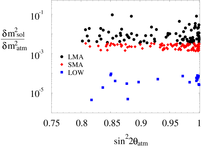
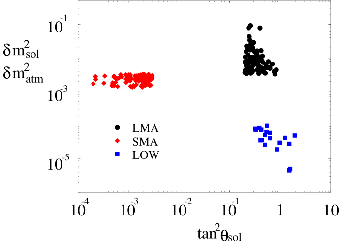
Figure 1: Distribution of the points of neutrino solutions in Model I. Black circles satisfy the constraints for the LMA solution, the diamond-shaped points for the SMA solution, and the square points for the LOW solution.

One interesting point is that most of the predicted values for $|U_{e3}^{MNS}|$ are larger than $10^{-2}$ (Fig. 2), so that the values $|U_{e3}^{MNS}|$ can be reached by future neutrino experiments [12]. Therefore the future precise measurement of $|U_{e3}^{MNS}|$ will be very important to test this class of models.

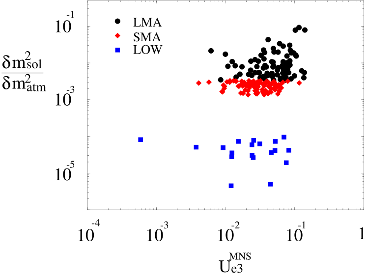
Figure 2: Predicted values of $|U_{e3}^{MNS}|$ in Model I

3.2 Model II $(\delta=0)$

In this case, all matrix elements in Eq. (11) with $\delta=0$ are of order 1, and hence we can expect all elements of the neutrino mixing matrix to be of order 1: $U^{MNS}_{ij}\sim O(1)~{}(i,j=1$–3). Therefore we can naturally get large mixing angles for both atmospheric and solar neutrinos. In our numerical analysis, we impose the same constraints for atmospheric, solar neutrino solutions and the CHOOZ experiment as in Model I. Then we search for the solutions. In Fig. 3, we show their distribution. As we expected, the SMA solution is hardly obtained, and it is difficult to make a large enough mass hierarchy for the LOW solution. Thus Model II strongly prefers the LMA solution. $0.01\%$ of the data sets passed the conditions for the LMA solution. The probability to realize the SMA and LOW solutions is very small. Therefore a near-future experiment, KamLAND [13], will be able to test this class of models. In Model II, the rate to realize the LMA solution is much smaller than in Model I. The main reason is that the limit on the CHOOZ experiment severely constrains the models, since the value of $U^{MNS}_{e3}$ tends to become of order 1. In Fig. 4, we show the predicted values of $U^{MNS}_{e3}$ for Model II. As can be seen from Fig. 4, the predicted values are so large that the future measurement of $U^{MNS}_{e3}$ can observe them [12]. Therefore, again the measurement of $U^{MNS}_{e3}$ is very important.

Another interesting possibility within Model II is that the inverted hierarchical neutrino masses, that is $m^{2}_{\nu 3}\ll m^{2}_{\nu 1}<m^{2}_{\nu 2}$ with $\delta m^{2}_{\rm atm}=m^{2}_{\nu 3}-m^{2}_{\nu 2}$ and $\delta m^{2}_{\rm sol}=m^{2}_{\nu 2}-m^{2}_{\nu 1}$, could be realized because of the degeneracy of the neutrino mass matrix elements. However, we checked that the rate to realize such a possibility is very small; only $2\times 10^{-3}~{}\%$ of the data sets passed the criterion of the inverted hierarchy and the constraints for the LMA solutions. This possibility can be tested by future neutrino experiments such as the neutrino factory [12], if this could be realized.

Here we mainly stressed the importance of the measurement of $U^{MNS}_{e3}$. In addition to this, CP violation and $2\beta 0\nu$ decay in neutrino physics are important to see the distinct features for Models I and II, as pointed out in Ref. [5].

In the next section, using the models that satisfied the neutrino constraints here, we will discuss in detail the LFV in the charged lepton sector.

Figure 3: Distribution of the points of neutrino solutions in Model II. All points satisfy the constraints for atmospheric and LMA solutions in Eqs. (20) and (21).

Figure 4: Predicted values of $|U_{e3}^{MNS}|$ in Model II

4 Lepton-Flavor Violation

In the presence of non-zero neutrino Yukawa couplings, we can expect LFV phenomena in the charged-lepton sector. Within the framework of SUSY models, flavor violation in neutrino Yukawa couplings induces LFV in slepton masses even if we assume the universal scalar mass for all scalars at GUT scale [7, 8]. In the present models, the LFV is generated in left-handed slepton masses since right-handed neutrinos couple to the left-handed lepton multiplets. A RG equation for the left-handed doublet slepton masses $(m^{2}_{\tilde{L}})$ can be written as

$$\mu\frac{d(m^{2}_{\tilde{L}})_{ij}}{d\mu} = \left(\mu\frac{d(m^{2}_{\tilde{L}})_{ij}}{d\mu}\right)_{\rm MSSM}$$ (28)

$$+\frac{1}{16\pi^{2}}\left[m^{2}_{\tilde{L}}f_{\nu}^{\dagger}f_{\nu}+f_{\nu}^{\dagger}f_{\nu}m^{2}_{\tilde{L}}+2(f_{\nu}^{\dagger}m^{2}_{\tilde{\nu}}f_{\nu}+\tilde{m}^{2}_{H_{u}}f_{\nu}^{\dagger}f_{\nu}+A_{\nu}^{\dagger}A_{\nu})\right]_{ij},$$

where $m^{2}_{\tilde{\nu}}$ and $\tilde{m}^{2}_{H_{u}}$ are soft SUSY-breaking masses for right-handed sneutrinos ($\tilde{\nu}$) and doublet Higgs ($H_{u}$), respectively. Here $(\mu d(m^{2}_{\tilde{L}})_{ij}/{d\mu})_{\rm MSSM}$ denotes the RG equation in case of the minimal SUSY SM (MSSM), and the terms explicitly written are additional contributions in the presence of the neutrino Yukawa couplings. In a basis where the charged-lepton Yukawa couplings are diagonal, the term $(\mu d(m^{2}_{\tilde{L}})_{ij}/{d\mu})_{\rm MSSM}$ does not provide any flavor violations. Therefore the only source of LFV comes from the additional terms. In our analysis, we numerically solve the RG equations, and then calculate the event rates for the LFV processes by using the complete formula in Ref. [8]. Here, in order to obtain an approximate estimation for the LFV masses, let us consider one-iteration approximate solution to the LFV mass terms ($i\neq j$):

$$(\Delta m^{2}_{\tilde{L}})_{ij}\simeq-\frac{(6+a_{0}^{2})m_{0}^{2}}{16\pi^{2}}(f_{\nu}^{\dagger}f_{\nu})_{ij}\log\frac{M_{G}}{M_{R}}.$$ (29)

Here we assume a universal scalar mass $(m_{0})$ for all scalars and a universal A-term $(A_{f}=a_{0}m_{0}f_{f})$ at the GUT scale ($M_{G}=2\times 10^{16}$ GeV). From Eqs. (7) and (15), the solution can be written as

$$(\Delta m^{2}_{\tilde{L}})_{ij}\simeq-\frac{(6+a_{0}^{2})m_{0}^{2}}{16\pi^{2}}U^{Dirac}_{ik}U^{Dirac*}_{jk}|f_{\nu k}|^{2}\log\frac{M_{G}}{M_{R}}.$$ (30)

Note that large neutrino Yukawa couplings and large lepton mixings $U^{Dirac}_{ij}$ generate the large LFV in the left-handed slepton masses.

The component $(\Delta m^{2}_{\tilde{L}})_{32}$ ($(\Delta m^{2}_{\tilde{L}})_{21}$) generates the $\tau\rightarrow\mu\gamma$ ($\mu\rightarrow e\gamma$) process through diagrams mediated by sleptons. The decay rates can be approximated as follows:

$${\rm\Gamma}(e_{i}\rightarrow e_{j}\gamma)\simeq\frac{e^{2}}{16\pi}m^{5}_{e_{i}}F\left|(\Delta m^{2}_{\tilde{L}})_{ij}\right|^{2}.$$ (31)

Here $F$ is a function of masses and mixings for SUSY particles. If the non-degeneracy of slepton masses is very small, the function $F$ is approximately process-independent.

Note that the mixing matrix that is relevant to the LFV masses is $U^{Dirac}$, not the neutrino mixing matrix $U^{MNS}$. The mixing matrix $U^{Dirac}$ depends on the FN charges of right-handed neutrinos $(a,b,c)$ and $\delta$. In the next subsections, we discuss the LFV in some interesting cases.

4.1 Model I ($\delta=1$) with $(a,b,c)=(0,1,2)$

First we discuss Model I ($\delta=1$) with $(a,b,c)=(0,1,2)$. In this case, the neutrino Dirac mass matrix in Eq. (7) is given by

$$m_{\nu D}=m_{3}\epsilon^{\tau}\left(\begin{array}[]{ccc}\bar{C}_{3}\epsilon^{3}&\bar{B}_{3}\epsilon^{2}&\bar{A}_{3}\epsilon^{2}\\ \bar{C}_{2}\epsilon^{2}&\bar{B}_{2}\epsilon&\bar{A}_{2}\epsilon\\ \bar{C}_{1}\epsilon&\bar{B}_{1}&\bar{A}_{1}\end{array}\right).$$ (35)

When we diagonalize the Dirac mass matrix, we get the following approximate expression for $U^{Dirac}$:

$$U^{Dirac} \simeq \left(\begin{array}[]{ccc}1&-\frac{\epsilon X}{\sqrt{1+|\bar{B}_{1}/\bar{A}_{1}|^{2}}}&\frac{\epsilon\bar{C}_{1}^{*}/\bar{A}_{1}^{*}}{\sqrt{1+|\bar{B}_{1}/\bar{A}_{1}|^{2}}}\\ \frac{\epsilon\bar{A}_{2}\bar{C}_{1}}{\bar{A}_{1}\bar{B}_{2}-\bar{B}_{1}\bar{A}_{2}}&\frac{1}{\sqrt{1+|\bar{B}_{1}/\bar{A}_{1}|^{2}}}&\frac{\bar{B}_{1}^{*}/\bar{A}_{1}^{*}}{\sqrt{1+|\bar{B}_{1}/\bar{A}_{1}|^{2}}}\\ -\frac{\epsilon\bar{B}_{2}\bar{C}_{1}}{\bar{A}_{1}\bar{B}_{2}-\bar{B}_{1}\bar{A}_{2}}&-\frac{\bar{B}_{1}/\bar{A}_{1}}{\sqrt{1+|\bar{B}_{1}/\bar{A}_{1}|^{2}}}&\frac{1}{\sqrt{1+|\bar{B}_{1}/\bar{A}_{1}|^{2}}}\end{array}\right),$$ (39)

where $X=\bar{C}_{1}^{*}(\bar{A}_{1}\bar{A}_{2}^{*}+\bar{B}_{1}\bar{B}_{2}^{*})/\bar{A_{1}}(\bar{A}_{1}^{*}\bar{B}_{2}^{*}-\bar{A}_{2}^{*}\bar{B}_{1}^{*})$. This expression is a leading order in terms of $\epsilon$. An important point is that the lepton mixing matrix $U^{Dirac}$ in Eq. (39) also contains a large mixing because of the lopsided structure of the Dirac neutrino masses.

The component $(\Delta m^{2}_{\tilde{L}})_{32}$ induces the $\tau\rightarrow\mu\gamma$ process. Taking into account the hierarchical structure of neutrino Yukawa couplings ($f_{\nu 1}:f_{\nu 2}:f_{\nu 3}\sim\epsilon^{2}:\epsilon:1$), a dominant term of the matrix element $(\Delta m^{2}_{\tilde{L}})_{32}$ can be written as

$$(\Delta m^{2}_{\tilde{L}})_{32} \simeq -\frac{(6+a_{0}^{2})m^{2}_{0}}{16\pi^{2}}U_{33}^{Dirac}U_{23}^{Dirac*}|f_{\nu 3}|^{2}\log\frac{M_{G}}{M_{R}}.$$ (40)

The component $(\Delta m^{2}_{\tilde{L}})_{21}$, on the other hand, generates the $\mu\rightarrow e\gamma$ process. Since $U_{13}^{Dirac}$ is of order $\epsilon$, a leading term of $(\Delta m^{2}_{\tilde{L}})_{21}$ can be written as

$$(\Delta m^{2}_{\tilde{L}})_{21} \simeq -\frac{(6+a_{0}^{2})m^{2}_{0}}{16\pi^{2}}U_{23}^{Dirac}U_{13}^{Dirac*}|f_{\nu 3}|^{2}\log\frac{M_{G}}{M_{R}}.$$ (41)

The branching ratio for the $\tau\rightarrow\mu\gamma$ ($\mu\rightarrow e\gamma$) process is proportional to the square of $(\Delta m^{2}_{\tilde{L}})_{32}$ ($(\Delta m^{2}_{\tilde{L}})_{21}$), as given in Eq. (31). Thus the important parameters for the branching ratios are the matrix elements $U^{Dirac}_{23}$, $U^{Dirac}_{13}$ and $U^{Dirac}_{33}$, and the third-generation Yukawa coupling $f_{\nu 3}$. In Model I, the element $U^{Dirac}_{23}$ is expected to be of order 1 because of the lopsided structure in the Dirac mass terms as expressed in Eq. (39). In Fig. 5, we show the numerical result for $U^{Dirac}_{23}$ compared to $U^{MNS}_{\mu 3}$. As expected from Eq. (39), $U^{Dirac}_{13}$ is of the order of $\epsilon$, as shown in Fig. 5.

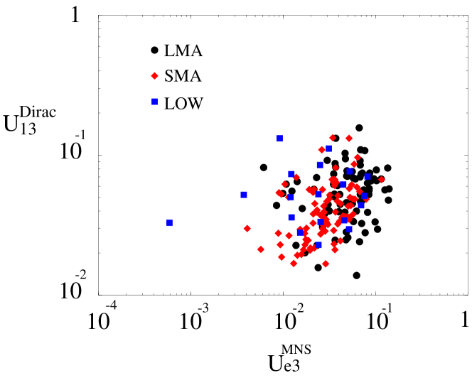
Figure 5: $U^{MNS}$ versus $U^{Dirac}$ in Model I with $(a,b,c)=(0,1,2)$.

The order-1 $U^{Dirac}_{23}$ and the order-$\epsilon$ (non-zero) $U^{Dirac}_{13}$ can induce a significantly large event rate for $\mu\rightarrow e\gamma$ process if the neutrino Yukawa coupling $f_{\nu 3}$ is large, as pointed out in Ref. [10].

A magnitude of $f_{\nu 3}$ depends on the FN charge $\tau$. Even at this stage, however, we can estimate the ratio of the branching ratios of the $\mu\rightarrow e\gamma$ and $\tau\rightarrow\mu\gamma$ processes as ${\rm Br}(\mu\rightarrow e\gamma)/{\rm Br}(\tau\rightarrow\mu\gamma)$, which is $\tau$-independent. If we consider a value of $\Gamma(e_{i}\rightarrow e_{j}\gamma)/\Gamma(e_{i}\rightarrow e_{j}\nu_{i}\bar{\nu}_{j})$, the dependence of the initial lepton mass in the process is cancelled. Thus we can expect the following relation from Eqs. (31), (40), and (41):

$$\frac{\Gamma(\mu\rightarrow e\gamma)/\Gamma(\mu\rightarrow e\nu_{\mu}\bar{\nu_{e}})}{\Gamma(\tau\rightarrow\mu\gamma)/\Gamma(\tau\rightarrow\mu\nu_{\tau}\bar{\nu_{\mu}})} \sim \left|\frac{(\Delta m^{2}_{\tilde{L}})_{21}}{(\Delta m^{2}_{\tilde{L}})_{32}}\right|^{2}\simeq\left|\frac{U^{Dirac}_{13}}{U^{Dirac}_{33}}\right|^{2}\sim\epsilon^{2}\left|\frac{\bar{C}_{1}}{\bar{A}_{1}}\right|^{2}.$$ (42)

Taking into account ${\rm Br}(\mu\rightarrow e\nu_{\mu}\bar{\nu_{e}})\simeq 100\%$ and ${\rm Br}(\tau\rightarrow\mu\nu_{\tau}\bar{\nu_{\mu}})\simeq 17\%$, we obtain

$$\frac{{\rm Br}(\mu\rightarrow e\gamma)}{{\rm Br}(\tau\rightarrow\mu\gamma)} \sim \frac{\epsilon^{2}}{0.17}\left|\frac{\bar{C}_{1}}{\bar{A}_{1}}\right|^{2}\sim 0.03\left(\frac{\epsilon}{0.07}\right)^{2}\left(\frac{|\bar{C}_{1}/\bar{A}_{1}|}{1.0}\right)^{2}.$$ (43)

This relation is a $\tau$-independent prediction of Model I with $(a,b,c)=(0,1,2)$. Since the current experimental limits on these processes are ${\rm Br}(\mu\rightarrow e\gamma)<1.2\times 10^{-11}$ and ${\rm Br}(\tau\rightarrow\mu\gamma)<1.1\times 10^{-6}$ [14], the process $\mu\rightarrow e\gamma$ is much more sensitive to this class of models.

In order to discuss the absolute values of the branching ratios for LFV processes, we need to fix the FN charge parameter $\tau$. In SUSY models, there are two interesting cases. In the models with $\tau=0$, it is suggested that all the third-generation Yukawa couplings are of order 1. In SUSY models, this is realized in the case with the large $\tan\beta$ ($\tan\beta\simeq 50$). In the models with $\tau=1$, all the third-generation Yukawa couplings are of order $\epsilon$, except the top Yukawa coupling, which is expected to be of order 1. This is likely to be the case with small $\tan\beta$ ($\tan\beta\simeq 5$) in SUSY models. Therefore, in the next subsections, we will consider the two cases, Case 1, $\tau=0$ and Case 2, $\tau=1$, to see how large the predicted branching ratios for LFV processes can be.

4.1.1 Case 1, $\tau=0$

In Case 1, the models suggest that all third-generation Yukawa couplings at the GUT scale are of order 1. Therefore, a large $\tan\beta$ is preferred. Here we take $\tan\beta=50$. In our numerical analysis, we impose $m_{3}=m_{\rm top}$ at GUT scale in the Dirac neutrino mass Eq. (35) with $\tau=0$, and then we require the neutrino mass squared difference to be $\delta m^{2}_{32}=3\times 10^{-3}$ eV² in order to fix the right-handed neutrino mass scale $M_{R}$. We have checked that all third-generation Yukawa couplings are of the same order, which is about 0.5–0.8. Since the third-generation neutrino Yukawa coupling is as large as the top Yukawa coupling, so the large LFV masses are generated through the RGE running. Furthermore, since $\tan\beta$ is very large, the low-energy amplitudes of LFV processes are enhanced. Therefore, we can expect very large branching ratios for LFV processes [10].

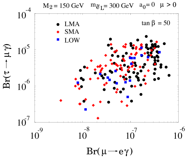
Figure 6: Br($\mu\rightarrow e\gamma$) versus Br($\tau\rightarrow\mu\gamma$) in Model I with $(a,b,c,\tau)=(0,1,2,0)$. Here we take the left-handed slepton mass to be 300 GeV, the Wino mass to be 150 GeV, and $\epsilon=0.07$.

Figure 7: Br($\mu\rightarrow e\gamma$) as a function of the left-handed selectron mass in Model I with $(a,b,c)=(0,1,2,0)$.

In Fig. 7, we show the numerical result for Br($\tau\rightarrow\mu\gamma$) and Br($\mu\rightarrow e\gamma$). Here the circle points satisfy the LMA solution for solar neutrinos, the diamond-shaped points the SMA solution, and the square points the LOW solution. As can be seen from the figure, the branching ratios for the LFV processes do not depend on the solar neutrino solutions since the important parameters for $\mu\rightarrow e\gamma$ and $\tau\rightarrow\mu\gamma$ branching ratios are only $U^{Dirac}_{13}$, $U^{Dirac}_{23}$ and $U^{Dirac}_{33}$, which are not affected very much by the constraints on solar neutrino solutions, as shown in Fig. 5. We also see that the estimation Eq. (43) is approximately correct, so that the limit from the $\mu\rightarrow e\gamma$ process can provide much stronger constraints on the models. In Fig. 7, we select one point from Fig. 7 and show the slepton mass dependence of the branching ratio for the $\mu\rightarrow e\gamma$ process. In this case, these branching ratios are too large to be consistent with the present experimental bounds. Therefore the large region of parameter space is already excluded.

These results illustrate the significant potential of the LFV searches to probe the realistic neutrino models.

4.1.2 Case 2, $\tau=1$

In models with $\tau=1$, the top Yukawa coupling is expected to be of order 1, while the other third-generation Yukawa couplings (bottom, tau and tau-neutrino Yukawa couplings) are of order $\epsilon$. It is thus likely to be the case with relatively small $\tan\beta$. Here we take $\tan\beta=5$, and we impose $m_{3}=m_{\rm top}$ at GUT scale in the Dirac neutrino mass matrix in Eq. (35) with $\tau=1$, in other words, $(f_{\nu})_{33}=\epsilon f_{top}\bar{A}_{1}$. We checked that in the case with $\tan\beta=5$, the bottom and tau Yukawa couplings approximately satisfy the condition $f_{b}\simeq f_{\tau}\simeq\epsilon f_{top}$. Therefore, as compared with the case with $\tau=0$, the LFV masses in Eqs. (40) and (41) are suppressed by $\epsilon^{2}$, and then the branching ratios for the $\tau\rightarrow\mu\gamma$ and $\mu\rightarrow e\gamma$ processes are reduced by $\epsilon^{4}$. The numerical results for the branching ratios are shown in Fig. 9.

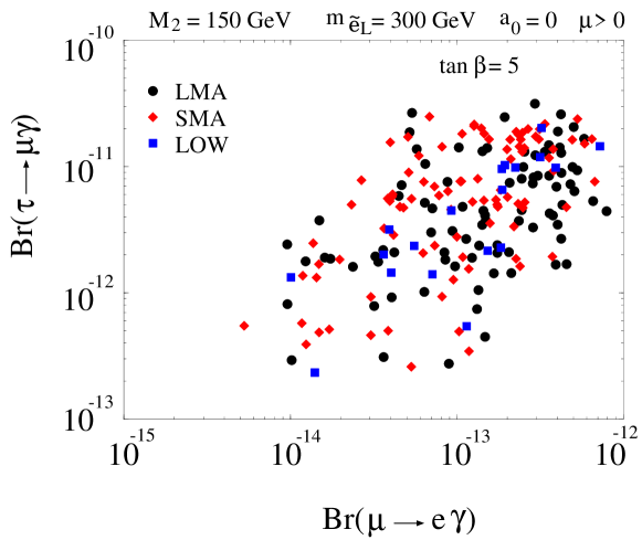
Figure 8: Br($\mu\rightarrow e\gamma$) versus Br($\tau\rightarrow\mu\gamma$) in Model I with $(a,b,c,\tau)=(0,1,2,1)$. Here we take the left-handed slepton mass to be 300 GeV, the Wino mass to be 150 GeV, and $\epsilon=0.07$.

Figure 9: Br($\mu\rightarrow e\gamma$) as a function of the left-handed selectron mass in Model I with $(a,b,c,\tau)=(0,1,2,1)$.

Note that the predicted branching ratios in all solar neutrino solutions are almost the same, and that the relation in Eq. (43) is approximately satisfied. Thus the $\mu\rightarrow e\gamma$ search is much more sensitive to this class of models, unless the future sensitivity of Br($\tau\rightarrow\mu\gamma$) can reach values much below $10^{-10}$. In Fig. 9 we also show the branching ratio for $\mu\rightarrow e\gamma$ as a function of the left-handed selectron mass. As can be seen from Figs. 9 and 9, it is very interesting that the predicted branching ratios for $\mu\rightarrow e\gamma$ can be just below the present experimental bound (Br$(\mu\rightarrow e\gamma)<1.2\times 10^{-11}$ [14]) in a wide range of parameter space. We also get the ratios between branching ratios Br($\mu\rightarrow eee$)/Br($\mu\rightarrow e\gamma$) and R($\mu\rightarrow e$ in Ti (Al))/Br($\mu\rightarrow e\gamma$) as follows:

$$\frac{{\rm Br}(\mu\rightarrow eee)}{{\rm Br}(\mu\rightarrow e\gamma)} \simeq 6\times 10^{-3},$$ (44)

$$\frac{{\rm R}(\mu\rightarrow e~{}{\rm in~{}Ti~{}(Al)})}{{\rm Br}(\mu\rightarrow e\gamma)} \simeq 5~{}(3)\times 10^{-3}.$$ (45)

In the present models, these ratios are quite predictive since the on-shell photon penguin diagram, which induces the $\mu\rightarrow e\gamma$ process, dominates over the other contributions to the $\mu\rightarrow eee$ and $\mu\rightarrow e$ conversion processes. Therefore the future improvements of the branching ratios, Br($\mu\rightarrow e\gamma)\sim 10^{-14}$ [15], and R($\mu\rightarrow e$ in Al$)\sim 10^{-16}$ [16] (and possibly R($\mu\rightarrow e$ in Ti$)\sim 10^{-18}$ [17]) will provide a significant impact to this class of models.

4.2 Model I with $(a,b,c)=(0,0,0)$

In this case, the Dirac neutrino mass matrix in Eq. (7) is given by

$$m_{\nu D}=m_{3}\epsilon^{\tau}\left(\begin{array}[]{ccc}\bar{C}_{3}\epsilon&\bar{B}_{3}&\bar{A}_{3}\\ \bar{C}_{2}\epsilon&\bar{B}_{2}&\bar{A}_{2}\\ \bar{C}_{1}\epsilon&\bar{B}_{1}&\bar{A}_{1}\end{array}\right).$$ (49)

Then we obtain the mixing matrix $U^{Dirac}$ as follows:

$$U^{Dirac} \simeq \left(\begin{array}[]{ccc}1&\epsilon\frac{X_{-}}{\sqrt{N_{-}}}&\epsilon\frac{X_{+}}{\sqrt{N_{+}}}\\ \epsilon Y_{0}&\frac{Y_{-}}{\sqrt{N_{-}}}&\frac{Y_{+}}{\sqrt{N_{+}}}\\ \epsilon Z_{0}&\frac{Z}{\sqrt{N_{-}}}&\frac{Z}{\sqrt{N_{+}}}\end{array}\right),$$ (53)

in the leading order of $\epsilon$. Here the coefficients $X_{\pm}$, $Y_{\pm(0)}$, $Z_{(0)}$, and $N_{\pm}$ are expressed by

$$Y_{0} = \frac{(\bar{A}_{i}\bar{B}_{i}^{*})(\bar{A}_{j}^{*}\bar{C}_{j})-(\bar{A}_{i}\bar{A}_{i}^{*})(\bar{B}_{j}^{*}\bar{C}_{j})}{(\bar{A}_{i}^{*}\bar{A}_{i})(\bar{B}_{j}^{*}\bar{B}_{j})-(\bar{A}_{i}\bar{B}^{*}_{i})(\bar{A}_{j}^{*}\bar{B}_{j})},~{}~{}Z_{0}=\frac{(\bar{A}_{i}^{*}\bar{B}_{i})(\bar{B}_{j}^{*}\bar{C}_{j})-(\bar{A}_{i}^{*}\bar{C}_{i})(\bar{B}_{j}^{*}\bar{B}_{j})}{(\bar{A}_{i}^{*}\bar{A}_{i})(\bar{B}_{j}^{*}\bar{B}_{j})-(\bar{A}_{i}\bar{B}^{*}_{i})(\bar{A}_{j}^{*}\bar{B}_{j})},$$

$$Y_{\pm} = \frac{-(\bar{A}_{i}^{*}\bar{A}_{i})+(\bar{B}_{i}^{*}\bar{B}_{i})\pm\sqrt{\left\{(\bar{A}_{i}^{*}\bar{A}_{i})-(\bar{B}_{i}^{*}\bar{B}_{i})\right\}^{2}+4(\bar{A}_{i}^{*}\bar{B}_{i})(\bar{A}_{j}\bar{B}_{j}^{*})}}{2},$$

$$Z = (\bar{A}_{i}^{*}\bar{B}_{i}),~{}~{}X_{\pm}=-Y_{\pm}Y_{0}^{*}-Z_{\pm}Z_{0}^{*},~{}~{}N_{\pm}=|Y_{\pm}|^{2}+|Z_{\pm}|^{2}.$$ (54)

Here summation over $i$ and $j$ $(i,j=1,2)$ is assumed: for example, $(\bar{A}_{i}^{*}\bar{B}_{i})\equiv\sum_{i=1-2}\bar{A}_{i}^{*}\bar{B}_{i}$. The main difference from that in the previous case (see Eq. (39)) is that the matrix elements $U^{Dirac}_{ij}$ depend on more parameters, since the matrix elements $(m_{\nu D})_{ij}~{}(i=1,2,~{}j=1-3)$ are larger than those in Eq. (35). However, the important point is the same, that is the matrix elements $U^{Dirac}_{ij}$ $(i,j=2,3)$ in Eq. (53) are of order 1 because of the lopsided structure of the Dirac neutrino mass matrix, and the element $U^{Dirac}_{13}$ is of order $\epsilon$.

In the present case, the feature of the LFV is very similar to the previous case: Model I with $(a,b,c)=(0,1,2)$. The hierarchy of neutrino Yukawa couplings is $f_{\nu 1}:f_{\nu 2}:f_{\nu 3}\sim\epsilon:\epsilon-1:1$, which depends on the solar neutrino solutions, and hence also the contributions induced by $f_{\nu 2}$ will be important. The leading contribution to the LFV mass $(\Delta m^{2}_{\tilde{L}})_{32}$ is given by

$$(\Delta m^{2}_{\tilde{L}})_{32} \simeq -\frac{(6+a_{0}^{2})m_{0}^{2}}{16\pi^{2}}\left[U^{Dirac}_{33}U^{Dirac*}_{23}|f_{\nu 3}|^{2}\right.$$ (55)

$$\left.\hskip 42.67912pt+U^{Dirac}_{32}U^{Dirac*}_{22}|f_{\nu 2}|^{2}\right]\log\frac{M_{G}}{M_{R}},$$

$$\sim -\frac{(6+a_{0}^{2})m_{0}^{2}}{16\pi^{2}}U^{Dirac}_{33}U^{Dirac*}_{23}\left(|f_{\nu 3}|^{2}-|f_{\nu 2}|^{2}\right)\log\frac{M_{G}}{M_{R}}.$$

In the SMA and LOW solutions, $|U^{Dirac}_{33}U^{Dirac}_{23}|\sim 0.5$ because of the lopsided structure of the Dirac neutrino mass matrix, and $(|f_{\nu 3}|^{2}-|f_{\nu 2}|^{2})/(|f_{\nu 1}|^{2}+|f_{\nu 2}|^{2}+|f_{\nu 3}|^{2})\sim 1$ since the mass scale for solar neutrinos is much smaller than the mass scale for atmospheric neutrinos (i.e. $|f_{\nu 3}|\gg|f_{\nu 2}|,~{}|f_{\nu 1}|$). On the other hand, in the LMA solution, $|U^{Dirac}_{33}U^{Dirac}_{23}|$ and $(|f_{\nu 3}|^{2}-|f_{\nu 2}|^{2})/(|f_{\nu 1}|^{2}+|f_{\nu 2}|^{2}+|f_{\nu 3}|^{2})$ can be widely spread since other matrix elements of $U^{Dirac}$ may have a large mixing and the mass scale for solar neutrinos can be close to the scale for atmospheric neutrinos. In Fig. 10, for example, we show the distribution of the values for $U^{Dirac}_{23}$ compared with the values for $U^{MNS}_{23}$. In the SMA and LOW solutions, $U^{Dirac}_{23}\simeq U^{MNS}_{\mu 3}$; on the other hand, the values for $U^{Dirac}_{23}$ in the LMA solution are widely distributed. Therefore, the values of the branching ratio for $\tau\rightarrow\mu\gamma$ in the case of the LMA solution can be much more broadly distributed than in the other cases.

The dominant contribution to the LFV mass $(\Delta m^{2}_{\tilde{L}})_{21}$ can be written as

$$(\Delta m^{2}_{\tilde{L}})_{21} \simeq -\frac{(6+a_{0}^{2})m_{0}^{2}}{16\pi^{2}}\left[U^{Dirac}_{23}U^{Dirac*}_{13}|f_{\nu 3}|^{2}\right.$$ (56)

$$\left.\hskip 42.67912pt+U^{Dirac}_{22}U^{Dirac*}_{12}|f_{\nu 2}|^{2}\right]\log\frac{M_{G}}{M_{R}},$$

$$= -\frac{(6+a_{0}^{2})m_{0}^{2}}{16\pi^{2}}\left[U^{Dirac}_{23}U^{Dirac*}_{13}\left(|f_{\nu 3}|^{2}-|f_{\nu 2}|^{2}\right)\right.$$

$$\left.\hskip 71.13188pt-U^{Dirac}_{21}U^{Dirac*}_{11}|f_{\nu 2}|^{2}\right]\log\frac{M_{G}}{M_{R}}.$$

In the cases of the SMA and LOW solutions, the first term in Eq. (56) is dominant since $|f_{\nu 3}|\gg|f_{\nu 2}|$ and $U^{Dirac}_{13}$ is non-negligible, as shown in Fig. 10. In the case of the LMA solution, the second term can be large since $f_{\nu 3}\sim f_{\nu 2}$ in order to get mass scale for the LMA solution, and $U^{Dirac}_{21}$ can be large because of the large mixing for the LMA solution. The matrix elements $|U^{Dirac}_{23}U^{Dirac}_{13}|$ and $|U^{Dirac}_{21}U^{Dirac}_{11}|$ are broadly distributed (for example, see in Fig. 10), and hence the value of the branching ratio for $\mu\rightarrow e\gamma$ can be widely distributed in all cases.

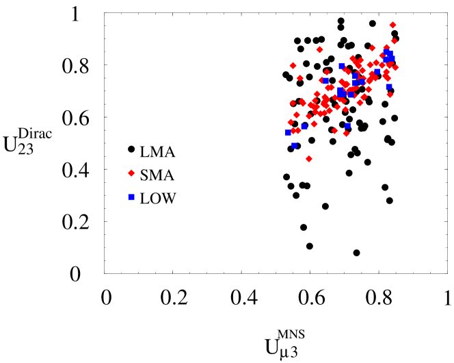
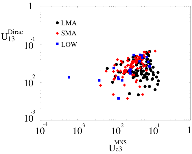
Figure 10: $U^{MNS}$ versus $U^{Dirac}$ in Model I with $(a,b,c)=(0,0,0)$.

When $|f_{\nu 3}|^{2}\gg|f_{\nu 2}|^{2}$, a ratio of branching ratios can be approximately as follows:

$$\frac{{\rm Br}(\mu\rightarrow e\gamma)}{{\rm Br}(\tau\rightarrow\mu\gamma)} \sim \frac{1}{0.17}\left|\frac{(\Delta m^{2}_{\tilde{L}})_{21}}{(\Delta m^{2}_{\tilde{L}})_{32}}\right|^{2}\sim 0.01\left|\frac{U^{Dirac}_{13}/0.03}{U^{Dirac}_{33}/0.7}\right|^{2}.$$ (57)

Taking into account the present experimental limits and the future expectation on these processes, the search for $\mu\rightarrow e\gamma$ can be much more sensitive to this class of models than the search for $\tau\rightarrow\mu\gamma$.

In the following subsections, in order to obtain the magnitude of the branching ratios for the LFV processes, we consider two cases again: Case 1, $\tau=0$ and Case 2, $\tau=1$.

4.2.1 Case 1, $\tau=0$

As in the previous models in section 4.1.1, we take $\tan\beta=50$ in order for all the third-generation Yukawa couplings to be of order 1. We assume that $m_{3}=m_{top}$ at the GUT scale in Eq. (49) with $\tau=0$. In Fig. 12 we show the result of the branching ratios for the $\tau\rightarrow\mu\gamma$ and $\mu\rightarrow e\gamma$ processes. Because of the large neutrino Yukawa coupling, the branching ratios of the $\mu\rightarrow e\gamma$ process are so large that most of the parameter region can be excluded by the present limit on $\mu\rightarrow e\gamma$. As in the models with the FN charges $(a,b,c)=(0,1,2)$, the models with $\tau=0$, which have a mild Yukawa unification between the top and tau-neutrino, are almost excluded by the bound on $\mu\rightarrow e\gamma$ [10].

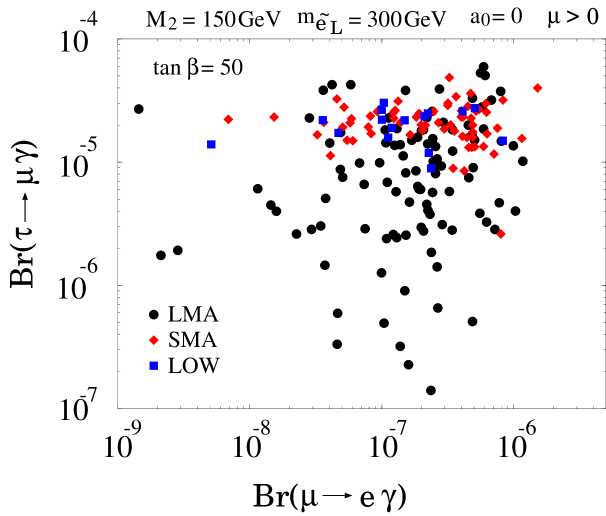
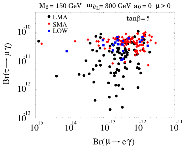
Figure 11: Br($\mu\rightarrow e\gamma$) versus Br($\tau\rightarrow\mu\gamma$) in Model I with $(a,b,c,\tau)=(0,0,0,0)$. Here we take the left-handed slepton mass to be 300 GeV, the Wino mass to be 150 GeV, and $\epsilon=0.07$.

   

Figure 12: Same as Fig.12 except for Model I with $(a,b,c,\tau)=(0,0,0,1)$.

4.2.2 Case 2, $\tau=1$

In the models with $\tau=1$, as discussed in section 4.1.2, the following relations among the third generation Yukawa couplings are implied: $f_{b}\sim f_{\tau}\sim f_{\nu 3}\sim\epsilon f_{top}$. Thus we assume that in Eq. (49) with $\tau=1$, $m_{3}=m_{top}$ at the GUT scale and take $\tan\beta$ to be 5 in order to realize the relation. As compared to the case with $\tau=0$, the branching ratios for $\tau\rightarrow\mu\gamma$ and $\mu\rightarrow e\gamma$ are suppressed by $\epsilon^{4}$, with the additional suppression due to small $\tan\beta$. In Fig. 12 we show the result of the branching ratios for $\tau\rightarrow\mu\gamma$ and $\mu\rightarrow e\gamma$. For the $\mu\rightarrow 3e$ and $\mu\rightarrow e$ conversion processes, we have checked that the relations in Eqs. (44) and (45) are held. Therefore, interestingly, the predicted event rates for $\mu\rightarrow e\gamma$ and $\mu\rightarrow e$ conversion can be as large as those the future experiments can reach. On the other hand, for $\tau\rightarrow\mu\gamma$ process, the significant improvement of the branching ratio sensitivity of much below $10^{-10}$ will be needed in order to reach the predicted values.

4.3 Model II ($\delta=0$) with $(a,b,c,\tau)=(0,1,2,1)$

Let us discuss the LFV in Model II ($\delta=0$). First we consider the case with hierarchical right-handed neutrino masses, that is the case with $(a,b,c)=(0,1,2)$. The Dirac neutrino mass matrix is given by

$$m_{\nu D}=m_{3}\epsilon\left(\begin{array}[]{ccc}\bar{C}_{3}\epsilon^{2}&\bar{B}_{3}\epsilon^{2}&\bar{A}_{3}\epsilon^{2}\\ \bar{C}_{2}\epsilon&\bar{B}_{2}\epsilon&\bar{A}_{2}\epsilon\\ \bar{C}_{1}&\bar{B}_{1}&\bar{A}_{1}\end{array}\right).$$ (61)

Since the matrix elements $(m_{\nu D})_{3i}/(m_{3}\epsilon)$ ($i=1$–3) are of order 1, we can expect that all elements of the mixing matrix $U^{Dirac}$ would be of order one: $U^{Dirac}_{ij}\sim O(1)$, even if we imposed the constraints of neutrino parameters on the neutrino mixing matrix $U^{MNS}$. This structure of the mixing matrix $U^{Dirac}$ is quite distinct from that in Model I, as seen in Eqs. (39) and (53). For example. in Fig. 13, we show $U^{Dirac}_{13}$ compared with $U^{Dirac}_{33}$. Even though the CHOOZ limit $|U^{MNS}_{e3}|<0.15$ was imposed, the component $U^{Dirac}_{13}$ can be of order 1. This large $U^{Dirac}_{13}$ is a very important feature for the LFV in the present models.

Figure 13: $U^{Dirac}_{13}$ versus $U^{Dirac}_{33}$ in Model II with $(a,b,c)=(0,1,2)$.

Because of the FN charges of right-handed neutrinos, the structure of neutrino Yukawa couplings is hierarchical ($f_{\nu 1}:f_{\nu 2}:f_{\nu 3}\sim\epsilon^{2}:\epsilon:1$). Therefore, only the third-generation Yukawa coupling $f_{\nu 3}$ is important for contributions to LFV masses. The dominant terms of the matrix elements ($(\Delta m^{2}_{\tilde{L}})_{32}$) and ($(\Delta m^{2}_{\tilde{L}})_{21}$) are given by

$$(\Delta m^{2}_{\tilde{L}})_{32} \simeq -\frac{(6+a_{0}^{2})m^{2}_{0}}{16\pi^{2}}U_{33}^{Dirac}U_{23}^{Dirac*}|f_{\nu 3}|^{2}\log\frac{M_{G}}{M_{R}},$$ (62)

$$(\Delta m^{2}_{\tilde{L}})_{21} \simeq -\frac{(6+a_{0}^{2})m^{2}_{0}}{16\pi^{2}}U_{23}^{Dirac}U_{13}^{Dirac*}|f_{\nu 3}|^{2}\log\frac{M_{G}}{M_{R}}.$$ (63)

Then a ratio of branching ratios Br($\mu\rightarrow e\gamma$)/Br($\tau\rightarrow\mu\gamma$) are approximately expressed as follows:

$$\frac{{\rm Br}(\mu\rightarrow e\gamma)}{{\rm Br}(\tau\rightarrow\mu\gamma)}\simeq\frac{1}{0.17}\left|\frac{(\Delta m^{2}_{\tilde{L}})_{21}}{(\Delta m^{2}_{\tilde{L}})_{32}}\right|^{2}\sim 6\left|\frac{U^{Dirac}_{13}}{U^{Dirac}_{33}}\right|^{2}.$$ (64)

Since $|U^{Dirac}_{13}|\sim|U^{Dirac}_{33}|$, as shown in Fig. 13, the branching ratio for $\mu\rightarrow e\gamma$ can be as large as or even larger than that for $\tau\rightarrow\mu\gamma$. As discussed in Model I, the models with $\tau=0$, in which a mild Yukawa unification between the top and tau-neutrino is realized, are almost excluded by the present $\mu\rightarrow e\gamma$ bound [10]. Therefore, in this section, we only present the result in the models with $\tau=1$.

In Fig. 14, we show the numerical result for these branching ratios. The predicted branching ratios for $\mu\rightarrow e\gamma$ are larger than those in Model I, since the mixing element $U^{Dirac}_{13}$ is much larger than that in the Model I. On the other hand, the branching ratios for $\tau\rightarrow\mu\gamma$ are almost the same as those in Model I. As expected, the predicted branching ratios for $\mu\rightarrow e\gamma$ are as large as those for $\tau\rightarrow\mu\gamma$. Note that for the $\mu\rightarrow 3e$ and $\mu\rightarrow e$ conversion processes, the relations in Eqs. (44) and (45) are predicted. Therefore the search for LFV in muon processes is much more sensitive to this class of models too. Even at present, some of the points in Fig. 14 are already excluded by the current experimental limit on $\mu\rightarrow e\gamma$ [Br$(\mu\rightarrow e\gamma)<1.2\times 10^{-11}$ [14]]. The future proposed improvement of the limit on LFV in muon processes will definitely provide a significant test of this class of models.

Figure 14: Br($\mu\rightarrow e\gamma$) versus Br($\tau\rightarrow\mu\gamma$) in Model II with $(a,b,c,\tau)=(0,1,2,1)$. Here we take the left-handed slepton mass to be 300 GeV, the Wino mass to be 150 GeV, and $\epsilon=0.07$.

4.4 Model II ($\delta=0$) with $(a,b,c,\tau)=(0,0,0,1)$

Next we consider the models in which the heavy right-handed neutrinos are nearly degenerate, that is the models with $(a,b,c)=(0,0,0)$. Again here we only discuss the case with $\tau=1$.

The Dirac neutrino mass matrix is given by

$$m_{\nu D}=m_{3}\epsilon\left(\begin{array}[]{ccc}\bar{C}_{3}&\bar{B}_{3}&\bar{A}_{3}\\ \bar{C}_{2}&\bar{B}_{2}&\bar{A}_{2}\\ \bar{C}_{1}&\bar{B}_{1}&\bar{A}_{1}\end{array}\right).$$ (68)

Figure 15: $U^{Dirac}_{13}$ versus $U^{Dirac}_{33}$ in Model II with $(a,b,c)=(0,0,0)$.

Figure 16: Br($\mu\rightarrow e\gamma$) versus Br($\tau\rightarrow\mu\gamma$) in Model II with $(a,b,c,\tau)=(0,0,0,1)$. Here we take the left-handed slepton mass to be 300 GeV, the Wino mass to be 150 GeV, and $\epsilon=0.07$.

As in the previous case of Model II, we expect $U^{Dirac}_{ij}\sim O(1)$. In this case, if coefficients $\bar{A}_{i}$, $\bar{B}_{i}$ and $\bar{C}_{i}$ are all real, $U^{Dirac}=U^{MNS}$. Thus, as shown in Fig. 15, the component $U^{Dirac}_{13}$ tends to be smaller than that in the previous case, because the constraint $|U^{MNS}_{e3}|<0.15$ slightly affects the value of $U^{Dirac}_{13}$. However, all components in the Dirac mass matrix Eq. (68) are of order one, and all Yukawa couplings $f_{\nu i}~{}(i=1$–3) can contribute to the LFV in slepton masses. Therefore, branching ratios of $\tau\rightarrow\mu\gamma$ and $\mu\rightarrow e\gamma$ can be larger than those in the previous case of Model II. We present the numerical result in Fig. 16. As can be seen in Fig. 16, the branching ratio for $\mu\rightarrow e\gamma$ can be as large as that of $\tau\rightarrow\mu\gamma$, because all components $V^{Dirac}$ can be of the same order. Many of the points are already excluded by the present experimental limit on the $\mu\rightarrow e\gamma$ process, and the future improvement will be able to test this class of models.

5 Conclusions

We discussed the neutrino masses and LFV in SUSY models with lopsided FN charges. For neutrino physics, we stressed the importance of the measurement of $U^{MNS}_{e3}$ in both Models I and II. In Model II, the LMA solution is strongly preferred so that the near-future KamLAND experiment could play a significant role for this class of models.

We also analyzed the LFV in detail within this framework. The present experimental limits on LFV processes almost excluded the models with $\tau=0$ in which a mild Yukawa coupling unification between the top and tau-neutrino is realized at the GUT scale. In the models with $\tau=1$, in which the tau-neutrino Yukawa coupling is suppressed by $\epsilon$ compared with the top Yukawa coupling, the predicted branching ratios for $\tau\rightarrow\mu\gamma$ are as large as or much less than $10^{-10}$, and hence a significant experimental improvement of the limit on the branching ratio is needed in order to reach the predictions of this framework. On the other hand, the predicted branching ratios for $\mu\rightarrow e\gamma$ and $\mu\rightarrow e$ conversion in nuclei can be as large as those the future proposed experiments can reach. Therefore, the future experiments can provide the significant test of this realistic framework for neutrino masses as well as charged lepton and quark masses.

References

- [1] Y. Fukuda et al. (The Super-Kamiokande collaboration), Phys. Lett. B436, 33 (1998), Phys. Rev. Lett. 81, 1562 (1998).
- [2] J. Sato and T. Yanagida, Phys. Lett. B430, 127 (1998); Nucl. Phys. B (Proc. Suppl.) 77, 293 (1999); W. Buchmüller and T. Yanagida, Phys. Lett. B445, 399 (1999); C.H. Albright, K.S. Babu and S.M. Barr, Phys. Rev. Lett. 81, 1167 (1998); N. Irges, S. Lavignac and P. Ramond, Phys. Rev. D58, 035003 (1998).
- [3] See, for example, K.S. Babu and S.M. Barr, Phys. Lett. B381, 202 (1996); S.M. Barr, Phys. Rev. D55, 1659 (1997); M.J. Strassler, in Proceedings of International Workshop on Perspectives of Strong Coupling Gauge Theories, edited by J. Nishimura and K. Yamawaki (World Scientific, Singapore, 1997); S.F. King, Phys. Lett. B439, 350 (1998); J.K. Elwood, N. Irges and P. Ramond, Phys. Rev. Lett. 81, 5064 (1998); Y. Nomura and T. Yanagida, Phys. Rev. D59, 017303 (1999); N. Haba, Phys. Rev. D59, 035011 (1999); Y. Grossman, Y. Nir and Y. Shadmi, JHEP 9810, 007 (1998); J. Ellis, G.K. Leontaris, S. Lola and D.V. Nanopoulos, Eur. Phys. J. C9, 389 (1999); M. Fukugita, M. Tanimoto and T. Yanagida, Phys. Rev. D59, 113016 (1999); F. Vissani, JHEP 9811, 025 (1998); A.S. Joshipura and S.D. Rindani, Eur. Phys. J. C14, 85 (2000); C.D. Froggatt, M. Gibson and H.B. Nielsen, Phys. Lett. B446, 256 (1999); L.J. Hall and N. Weiner, Phys. Rev. D60, 033005 (1999); Z. Berezhiani and A. Rossi, JHEP 9903, 002 (1999); K. Hagiwara and N. Okamura, Nucl. Phys. B548, 60 (1999); G. Altarelli and F. Feruglio, Phys. Lett. B451, 388 (1999); K.S. Babu, J.C. Pati and F. Wilczek, Nucl. Phys. B566, 33 (2000); M. Tanimoto, Phys. Lett. B456, 220 (1999); S. Lola and G.G. Ross, Nucl. Phys. B553, 81 (1999); Y. Nomura and T. Sugimoto, Phys. Rev. D61, 093003 (2000); T. Blažek, S. Raby and K. Tobe, Phys. Rev. D60, 113001 (1999); Phys. Rev. D62, 055001 (2000); N. Arkani-Hamed and M. Schmaltz, Phys. Rev. D61, 033005 (2000); R. Barbieri, P. Creminelli and A. Romanino, Nucl. Phys. B559, 17 (1999); M. Tanimoto, T. Watari and T. Yanagida, Phys. Lett. B461, 345 (1999); K. Yoshioka, Mod. Phys. Lett. A15, 29 (2000); K.S. Babu and R.N. Mohapatra, Phys. Rev. Lett. 83, 2522 (1999); G. Altarelli, F. Feruglio and I. Masina, Phys. Lett. B472, 382 (2000); E. Ma, Phys. Rev. D61, 033012 (2000); A. Aranda, C.D. Carone and R.F. Lebed, Phys. Lett. B474, 170 (2000); P.H. Frampton and A. Rasin, Phys. Lett. B478, 424 (2000); R. Dermisek and S. Raby, Phys. Rev. D62, 015007 (2000); E.A. Mirabelli and M. Schmaltz, Phys. Rev. D61, 113011 (2000); L.J. Hall, H. Murayama and N. Weiner, Phys. Rev. Lett. 84, 2572 (2000); M. Bando, T. Kugo and K. Yoshioka, Prog. Theor. Phys. 104, 211 (2000); Phys. Lett. B483, 163 (2000); A. Nelson and M.J. Strassler, JHEP 0009, 030 (2000); R. Kitano and Y. Mimura, Phys. Rev. D63, 016008 (2001); N. Haba and H. Murayama, hep-ph/0009174.
- [4] C.D. Froggatt and H.B. Nielsen, Nucl. Phys. B147, 277 (1979).
- [5] J. Sato and T. Yanagida, Phys. Lett. B493, 356 (2000).
- [6] W. Buchmüller and T. Yanagida in Ref. [2]; T. Asaka, K. Hamaguchi, M. Kawasaki and T. Yanagida, Phys. Rev. D61, 083512 (2000).
- [7] F. Borzumati and A. Masiero, Phys. Rev. Lett. 57, 961 (1986).
- [8] J. Hisano, T. Moroi, K. Tobe, M. Yamaguchi and T. Yanagida, Phys. Lett. B357, 579 (1995); J. Hisano, T. Moroi, K. Tobe and M. Yamaguchi, Phys. Rev. D53, 2442 (1996).
- [9] J. Hisano, D. Nomura and T. Yanagida, Phys. Lett. B437, 351 (1998); J. Hisano and D. Nomura, Phys. Rev. D59, 116005 (1999); M.E. Gomez, G.K. Leontaris, S. Lola and J.D. Vergados, Phys. Rev. D59, 116009 (1999);W. Buchmüller, D. Delphine and F. Vissani, Phys. Lett. B459, 171 (1999); W. Buchmüller, D. Delphine and L.T. Handoko, Nucl. Phys. B576, 445 (2000); J. Ellis, M.E. Gomez, G.K. Leontaris, S. Lola and D.V. Nanopoulos, Eur. Phys. J. C14, 319 (2000); J.L. Feng, Y. Nir and Y. Shadmi, Phys. Rev. D61, 113005 (2000); S. Baek, T. Goto, Y. Okada and K. Okumura, hep-ph/0002141.
- [10] J. Sato, K. Tobe, and T. Yanagida, hep-ph/0010348, to appear in Phys. Lett. B.
- [11] T. Yanagida, in Proceedings of the Workshop on Unified Theory and Baryon Number of the Universe, edited by O. Sawada and A. Sugamoto, Report KEK-79-18 (1979); M. Gell-Mann, P. Ramond and R. Slansky, in Supergravity, edited by D.Z. Freedman and P. van Nieuwenhuizen (North-Holland, Amsterdam, 1979)
- [12] See, for example, Neutrino Factory and Muon Collider Collaboration (D. Ayres et al.), physics/9911009; (C. Albright et al.), hep-ex/0008064; Y. Obayashi, talk given at the Joint U.S/Japan Workshop On New Initiatives In Muon Lepton Flavor Violation and Neutrino Oscillation With High Intense Muon and Neutrino Sources, Honolulu, Hawaii, Oct. 2-6, 2000, http://meco.ps.uci.edu/lepton_workshop/talks/obayashi.pdf. See also the webpage of “Neutrino factory and muon storage rings at CERN”; http://muonstoragerings.web.cern.ch/muonstoragerings/
- [13] The KamLAND proposal, Stanford-HEP-98-03. See also the webpage: http://www.awa.tohoku.ac.jp/html/KamLAND/index.html.
- [14] J. Bartels et al. (Particle Data Group), Eur. Phys. J. C15, 1 (2000).
- [15] L.M. Barkov et al., Research Proposal to PSI, 1999. See the webpage: http://www.icepp.s.u-tokyo.ac.jp/meg.
- [16] MECO Collaboration, M. Bachman et al., Proposal to BNL, 1997. See also http://meco.ps.uci.edu.
- [17] For example, see technical notes in the homepage of the PRISM project; http://psux1.kek.jp/~prism. See also the webpage of “Neutrino factory and muon storage rings at CERN”; http://muonstoragerings.web.cern.ch/muonstoragerings/