M. Wakamatsu

PACS numbers : 12.39.Fe, 12.39.Ki, 12.38.Lg, 13.88.+e, 13.87.Fh

Abstract

It is widely believed that the transversity distribution function $h_{1}(x)$ provides us with valuable information for our thorough understanding of internal nucleon spin structure [1]. Because of its chiral-odd nature, however, it does not appear in the standard deep-inelastic inclusive cross sections (at least in the chiral limit). The only practical way to determine it has been believed to use Drell-Yang processes. Recently, the HERMES collaboration proved for the first time that it is practically feasible to measure chiral-odd distribution functions by making use of the so-called Collins mechanism [2] in the semi-inclusive electro-pion productions [3]. The first HERMES measurement of the azimuthal single target-spin asymmetries for charged pions has been done by using longitudinally polarized proton target. From the theoretical viewpoint, much simpler would be the measurement of the similar asymmetry for the target polarized transversely to the incident electron beam, since it enables us to determine the transversity distribution $h_{1}(x)$ more directly and efficiently. Such measurement will in fact be performed soon.

In view of this very exciting experimental situation, it is highly desirable to give some reliable predictions for the chiral-odd distribution functions of the nucleon. Naturally, complete understanding of the parton distribution functions (PDF) need to solve nonperturbative QCD dynamics. Unfortunately, the direct evaluation of the PDF in the lattice QCD simulation is not possible yet. At the present moment, we must therefore rely upon some effective theory of QCD. We would claim that, among many of them, most promising would be the chiral quark soliton model (CQSM) [5]-[9]. In fact, a prominent feature of the CQSM is that it can simultaneously explain two biggest findings in the recent experimental studies of high-energy deep-inelastic scattering observables, i.e. the EMC measurement in 1988 [10], which dictates unexpectedly small quark spin fraction of the nucleon, and the NMC measurement in 1991, which has revealed the excess of $\bar{d}$ sea over the $\bar{u}$ sea in the proton [11]. Furthermore, its unique prediction, i.e. the flavor asymmetry of the spin-dependent sea-quark distribution $\Delta\bar{u}(x)-\Delta\bar{d}(x)>0$ [12],[13], seems to win some semi-phenomenological and/or semi-theoretical support [14], although not entirely definite yet.

What is the chiral quark soliton model, then? For large enough $N_{c}$, a nucleon in this model is thought to be a composite of $N_{c}$ valence quarks and infinitely many Dirac sea quarks bound by the self-consistent pion field of hedgehog shape [5]. After canonically quantizing the spontaneous rotational motion of the symmetry breaking mean field configuration, we can perform nonperturbative evaluation of any nucleon observables with full inclusion of valence and deformed Dirac-sea quarks [6]. This incomparable feature of the model enables us to make a reasonable estimation not only of quark distributions but also of antiquark ones, as we shall demonstrate later. Finally, but most importantly, only 1 parameter of the model (dynamically generated quark mass $M$) was already fixed by low energy phenomenology, which means that we can give parameter-free predictions for parton distribution functions at the low renormalization scale. There already exist some investigations of the chiral-odd distribution functions based on the CQSM (or the Nambu-Jona-Lasinio soliton model). The first investigation of the transversity distribution $h_{1}(x)$ in the CQSM was done by Pobylitsa and Polyakov [15]. Although pioneering, their investigation should be taken as qualitative in several respects. First, the effect of vacuum polarization is entirely neglected. Second, only the isovector combination of $h_{1}(x)$, i.e. $h_{1}^{u}(x)-h_{1}^{d}(x)$, was estimated, and the isocalar piece $h_{1}^{u}(x)+h_{1}^{d}(x)$, which arises only at the subleading order of $1/N_{c}$ expansion, was left over. On the other hand, Gamberg et al. investigated both of $h_{1}^{u/d}(x)$ and $h_{L}^{u/d}(x)$, but also within the “valence-quark-only” approximation [16]. We shall later show that this approximation does not make full use of the potential power of the model and cannot be justified. The purpose of the present investigation is to give more complete predictions for the chiral-odd distribution functions with full inclusion of the vacuum polarization effects as well as the subleading $1/N_{c}$ corrections.

We start with the standard definition of the chiral-odd spin-dependent PDF [1] :

$$\!\!\!h_{1}^{(I=0/I=1)}(x)\ \equiv\ h_{1}^{u}(x)\pm h_{1}^{d}(x)\ =\ \frac{1}{4\,\pi}\,\int_{-\infty}^{\infty}\,dz_{0}\,\,e^{ixM_{N}z_{0}}$$

$$\times\ \langle N(\mbox{\boldmath$P$}=0)S_{\perp}\,|\,\psi^{\dagger}(0)\left(1+\gamma^{0}\gamma^{3}\right)\,\gamma_{\perp}\,\gamma_{5}\,\left\{\begin{array}[]{c}1\\ \tau_{3}\\ \end{array}\right\}\,\psi(z)\,|\,N(\mbox{\boldmath$P$}=0)S_{\perp}\rangle|_{z_{3}=-z_{0},z_{\perp}=0},\hskip 28.45274pt$$

$$\!\!\!h_{L}^{(I=0/I=1)}(x)\ \equiv\ h_{L}^{u}(x)\pm h_{L}^{d}(x)\ =\ \frac{1}{4\,\pi}\,\int_{-\infty}^{\infty}\,dz_{0}\,\,e^{ixM_{N}z_{0}}$$

$$\times\ \langle N(\mbox{\boldmath$P$}=0)S_{z}\,|\,\psi^{\dagger}(0)\,\gamma^{3}\,\gamma_{5}\,\left\{\begin{array}[]{c}1\\ \tau_{3}\\ \end{array}\right\}\,\psi(z)\,|\,N(\mbox{\boldmath$P$}=0)S_{z}\rangle|_{z_{3}=-z_{0},z_{\perp}=0}.$$ (6)

What we must evaluate here is the nucleon matrix elements of quark bilinear operators with light-cone separation. As fully discussed in [8],[9], on the basis of the path integral formulation of the CQSM, such nonlocality effects in time and spatial coordinates can be treated in a satisfactory way. Omitting the detail, we just recall here the fact that, within the framework of the CQSM, the isoscalar and isovector distributions have totally dissimilar theoretical structure since they have different dependence on the collective angular velocity $\Omega$ :

$$h_{1/L}^{u}(x)\ +\ h_{1/L}^{d}(x) {\sim} \,N_{c}\,\,O(\Omega^{1})\hskip 68.2866pt\sim\ O(N_{c}^{0})\,,$$ (7)

$$h_{1/L}^{u}(x)\ -\ h_{1/L}^{d}(x) {\sim} N_{c}\,[\,O(N_{c}^{1})\ +\ O(\Omega^{1})\,]\ \sim\ O(N_{c}^{1})\ +\ O(N_{c}^{0}),$$ (8)

where use has been made of the fact that $\Omega$ scales as $1/N_{c}$. A noteworthy feature here is the existence of the subleading $1/N_{c}$ correction to the isovector combination of the distributions. Its importance is already known from a similar analysis for the isovector longitudinally polarized distribution [9] or its first moment, i.e. the isovector axial coupling constant of the nucleon [17].

We summarize in Fig.1 the theoretical predictions for the chiral-odd distribution functions $h_{1}(x)$ and $h_{L}(x)$. Fig.1(a) and Fig.1(b) respectively stand for the isoscalar and isovector combinations of $h_{1}^{u}(x)$ and $h_{1}^{d}(x)$, while (c) and (d) represent the similar combinations of $h_{L}^{u}(x)$ and $h_{L}^{d}(x)$. Here, the distribution functions with negative $x$ should be interpreted as aitiquark ones according to the rule :

$$h_{1/L}^{u}(-x)\ \pm\ h_{1/L}^{d}(-x)\ =\ -\,\,[\,h_{1/L}^{\bar{u}}(x)\ \pm\ h_{1/L}^{\bar{d}}(x)\,]\hskip 28.45274pt(0<x<1).$$ (9)

In all the figures, the long-dashed curves peaked around $x\sim 1/3$ represent the contributions of $N_{c}$ valence quarks, while the dash-dotted curves are those of Dirac-sea quarks in the hedgehog mean field. The sums of these two contributions are denoted by solid curves. Concerning the transversity distributions $h_{1}(x)$, one sees that the effects of Dirac-sea quarks are not very large. One also notices that both of $h_{1}^{u}(x)+h_{1}^{d}(x)$ and $h_{1}^{u}(x)-h_{1}^{d}(x)$ have fairly small support in the negative $x$ region, which means that the transversity distributions do not have significant antiquark components, in contrast to the unpolarized as well as the longitudinally polarized distributions. Turning to the twist-3 distribution $h_{L}(x)$, one finds that the effect of Dirac-sea quarks are sizably large. Nevertheless, an interesting feature is that a considerable cancellations occurs between the contributions of valence quarks and of Dirac-sea quarks in the negative $x$ region. As a consequence, the antiquark components are not so significant also in the case of $h_{L}(x)$.

Figure 1: Theoretical predictions for the chiral-odd distributions $h_{1}(x)$ and $h_{L}(x)$. (a) and (b) respectively represent the isoscalar and isovector parts of $h_{1}(x)$, while (c) and (d) are the isoscalar and isovector parts of $h_{L}(x)$. In all the figures, the long-dashed and dash-dotted curves denote the contributions of $N_{c}$ valence quarks and of the Dirac-sea quarks, whereas the solid curves are the sum of these two contributions.

The transversity distribution $h_{1}^{q}(x)$ is of special importance, since it forms the set of twist-2 distribution functions, together with the unpolarized distributions $f_{1}^{q}(x)$ and the longitudinally polarized ones $g_{1}^{q}(x)$. It is known that these distribution functions must satisfy the so-called Soffer inequality [18] expressed in the following form :

$$|h_{1}^{q}(x)|\ \leq\ \frac{1}{2}\,\left(\,\pm\,f_{1}^{q}(x)\ +\ g_{1}^{q}(x)\right)\hskip 28.45274pt\left(x>0,\,x<0\right).$$ (10)

Here, the plus sign of $f_{1}^{q}(x)$ corresponds to the region $x>0$, while the minus sign to $x<0$. (Note that the inequality with negative argument gives a relation for the antiquark distributions.) Now the question is whether the predictions of the CQSM fulfill this general inequality or not. Fig.2 shows that, if one includes the vacuum polarization effects properly, the Soffer inequality is well satisfied for both of the $u$-quark and the $d$-quark. On the other hand, if one neglects the Dirac-sea contributions, it is badly broken for the antiquark distributions. An important lesson learned from this observation is that the field theoretical nature of the model, i.e. the proper inclusion of the vacuum polarization effects, plays essential roles in giving reasonable predictions for antiquark distributions. Another lesson is that the frequently-used saturation Ansatz of this inequality for estimating $h_{1}^{q}(x)$ is not justified. This seems reasonable to us, since the magnitude of $f_{1}^{q}(x)$ is much larger than $g_{1}^{q}(x)$ and since $h_{1}^{q}(x)$ is closer to $g_{1}^{q}(x)$ rather than $f_{1}^{q}(x)$.

Figure 2: Theoretical check of the Soffer inequality. (a) and (b) are the results obtained with full inclusion of the vacuum polarization effects, while (c) and (d) are obtained with “valence-quark-only” approximation. In all the figures, the solid and dashed curves represent the r.h.s and the l.h.s. of the inequality (6), respectively.

As already touched upon, HERMES group recently carried out a very interesting measurements on single target-spin asymmetries in semi-inclusive pion electroproduction [3]. What they have measured are the azimuthal asymmetries, i.e. the asymmetries of the cross sections depending on the azimuthal angle $\phi$ with respect to the lepton scattering plane :

$$A_{UL}^{W}\ =\ \frac{\int d\phi\,dy\,\,W(\phi)\,\,(d\sigma^{+}/S_{H}^{+}\,\,dx\,dy\,d\phi\ -\ d\sigma^{-}/S_{H}^{-}\,\,dx\,dy\,d\phi)}{\frac{1}{2}\,\,\int d\phi\,dy\,\,(d\sigma^{+}/S_{H}^{+}\,\,dx\,dy\,d\phi\ +\ d\sigma^{-}/S_{H}^{-}\,\,dx\,dy\,d\phi)},$$ (11)

with $W(\phi)=\sin\phi$ or $\sin 2\phi$ and with $S_{H}^{\pm}$ being the nucleon polarization. The theoretical analyses of these azimuthal asymmetries were already performed by several authors [19]-[23]. Here we use the expression given in [23] :

$$A^{\sin\phi} \simeq \,\frac{2\,M_{h}}{\langle\,P_{hT}\rangle}\cdot\langle\frac{|P_{hT}|}{M_{h}}\,\,\sin\phi\,\rangle\ \ \ \ \ \,=\ \frac{2\,M_{h}}{\langle P_{hT}\rangle}\cdot\frac{I_{2}(x,y,z)}{I_{1}(x,y,z)},$$ (12)

$$A^{\sin 2\,\phi} \simeq \frac{2\,M\,M_{h}}{\langle\,P_{hT}^{2}\rangle}\cdot\langle\frac{{|P_{hT}|}^{2}}{M\,M_{h}}\,\,\sin 2\,\phi\rangle\ =\ \frac{2\,M\,M_{h}}{\langle P_{hT}^{2}\rangle}\cdot\frac{I_{3}(x,y,z)}{I_{1}(x,y,z)},$$ (13)

where

$$I_{1}(x,y,z) = \frac{1}{2}\,\,\left[1+{(1-y)}^{2}\right]\,\,\sum_{a}\,e_{a}^{2}\,\,x\,f_{1}^{a}(x)\,\,D_{1}^{a}(z),$$ (14)

$$I_{2}(x,y,z) = 2\,(2-y)\,\frac{M}{Q}\,\,\sum_{a}\,e_{a}^{2}\,\,\left\{\,x^{2}\,h_{L}^{a}(x)\cdot z\,H_{1}^{\perp(1)a}(z)\ -\ x\,h_{1L}^{\perp(1)a}(x)\cdot\tilde{H}^{a}(z)\,\right\}$$ (15)

$$+ \!\!\sqrt{1-y}\,\,(1-y)\,\,\frac{2\,M\,x}{Q}\,\,\sum_{a}\,e_{a}^{2}\,\,x\,h_{1}^{a}(x)\cdot z\,H_{1}^{\perp(1)a}(z),$$

$$I_{3}(x,y,z) = 4\,(1-y)\,\,\sum_{a}\,\,e_{a}^{2}\,\,x\,h_{1L}^{\perp(1)a}(x)\cdot z^{2}\,H_{1}^{\perp(1)a}(z),$$ (16)

with $x=Q^{2}/2(P\cdot q),y=(P\cdot q)/(P\cdot k_{1})$ and $z=(P\cdot P_{h})/(P\cdot q)$ in the notation of [23]. One realizes that the asymmetries depend on 4 distribution functions $f_{1}(x),h_{1}(x),h_{L}(x),h_{1L}^{\perp(1)}(x)$ and 3 fragmentation functions $D_{1}(z),H_{1}^{\perp(1)}(z),\tilde{H}(z)$. Here $D_{1}(z)$ is the familiar spin-independent fragmentation function, while $H_{1}^{\perp(1)}(z)$ is $(k_{T}^{2}/2M_{h}^{2})$-weighted fragmentation function defined by

$$H_{1}^{\perp(1)a}(z)\ \equiv\ \int\,d^{2}\mbox{\boldmath$k$}^{\prime}_{T}\,\,\frac{|\mbox{\boldmath$k$}_{T}|^{2}}{2\,M_{h}^{2}}\,\,H_{1}^{\perp a}(z,k_{T}^{\prime}),$$ (17)

with $\mbox{\boldmath$k$}_{T}^{\prime}=-z\mbox{\boldmath$k$}_{T}$, where $H_{1}^{\perp q}(z,\mbox{\boldmath$k$}_{T}^{\prime})$ is a $T$(time-reversal)-odd leading twist fragmentation function, giving the probability of a spinless or unpolarized hadron to be created from a transversely polarized scattered quark. The remaining subleading $T$-odd fragmentation function $\tilde{H}^{a}(z)$ is known to be constrained by the relation $\tilde{H}^{a}(z)=z\,\frac{d}{dz}\left(zH_{1}^{\perp(1)a}(z)\right)$ due to the Lorentz invariance [20]. To estimate these T-odd fragmentation functions, we follow [22]-[23] and use the Collins Ansatz [2]

$$A_{C}(z,\mbox{\boldmath$k$}_{T})\ \equiv\ \frac{|\mbox{\boldmath$k$}_{T}|}{M_{h}}\cdot\frac{H_{1}^{\perp}(z,\mbox{\boldmath$k$}_{T}^{2})}{D_{1}(z,\mbox{\boldmath$k$}_{T}^{2})}\ =\ \eta\,\,\frac{M_{C}|\mbox{\boldmath$k$}_{T}|}{M_{C}^{2}+\mbox{\boldmath$k$}_{T}^{2}},$$ (18)

with the parameters $M_{C}=2\,m_{\pi}$ and $\eta=1.0$.

Coming back to the distribution functions, we need 4 functions $f_{1}(x),h_{1}(x),h_{L}(x)$ and $h_{1L}^{\perp(1)}(x)$. In the following, simply by using the GRV parameterization of the unpolarized distribution $f_{1}^{a}(x)$ [24], we concentrate on the chiral-odd distributions. Here, $h_{1}^{a}(x)$ is the familiar transversity distribution function. The function $h_{L}(x)$ consists of the twist-2 part, which is expressed by $h_{1}^{a}(x)$, and the interaction dependent part or the genuine twist-3 part, as

$$h_{L}^{a}(x)\ =\ 2\,x\,\,\int_{x}^{1}\,\,dy\,\,\frac{h_{1}^{a}(y)}{y^{2}}\ +\ \bar{h}_{L}^{a}(x).$$ (19)

On the other hand, the third function $h_{1L}^{\perp(1)a}(x)$ is expressed with use of $h_{1}^{a}(x)$ and $h_{L}^{a}(x)$ as

$$h_{1L}^{\perp(1)a}(x)\ =\ \int_{x}^{1}\,\,dy\,\,\left[\,h_{L}^{a}(y)\ -\ h_{1}^{a}(y)\,\right].$$ (20)

In the absence of powerful theories, the following two approximations have been frequently used for estimating these functions. The first is the twist-2 or the Wandzura-Wilczek type approximation for $h_{L}^{a}(x)$, i.e. the approximation to set $\bar{h}_{L}^{a}(x)\simeq 0$. The second approximation is to assume approximate equality of $h_{1}^{q}(x)$ and $h_{L}^{a}(x)$, which leads to $h_{1L}^{\perp(1)a}(x)\simeq 0$. This second approximation is advocated by HERMES group, by the reason that it seems consistent with small $\sin 2\phi$ asymmetry obtained by their experiment [22]-[23].

Since the CQSM can give some reasonable predictions for both of $h_{1}(x)$ and $h_{L}(x)$, the other distributions can also be determined by using (16). Fig.3 summarizes the theoretical predictions of the CQSM for these chiral-odd distributions with different flavors. The distributions shown here corresponds to the energy scale of $Q^{2}=2.5\,\mbox{GeV}^{2}$, an average value for the HERMES kinematical region. The scale dependencies of the distribution functions are taken into account in the following way. First, to include the scale dependencies of $h_{1}(x)$ and the twist-2 part of $h_{L}(x)$, we use the Fortran program of leading-order DGLAP equation [25]. On the other hand, the scale dependence of the twist-3 part of $h_{L}(x)$, i.e. $\bar{h}_{L}(x)$, is taken into account by solving the leading-order DGLAP type equation obtained in the large $N_{c}$ limit [26],[27]. The starting energy of these evolutions is taken to be $Q^{2}=0.23\,\mbox{GeV}^{2}$ [28]. From Fig.3(a) and 3(b), one reconfirms sizable differences between the two distributions $h_{1}(x)$ and $h_{L}(x)$, especially at lower values of $x$. A general tendency is that $h_{L}(x)$ is concentrated in the lower $x$ region as compared with $h_{1}(x)$. We recall that this characteristic is also observed in the MIT bag model predictions for the same distributions. In fact, the chiral-odd distributions $h_{1}(x)$ and $h_{L}(x)$ in both models are not extremely different as far as the dominant $u$-quark distribution in the proton is concerned. (This is not necessarily true for the corresponding $d$-quark distributions as well as the $\bar{u}$ and $\bar{d}$ ones. We also recall that the situation is quite different for the other two twist-2 distributions, i.e. the longitudinally polarized one and the unpolarized one.) The sizable difference between $h_{1}(x)$ and $h_{L}(x)$ indicates that the Ansatz $h_{1}(x)\simeq h_{L}(x)$ adopted by the HERMES group may not be necessarily justified. To verify it, we plot in Fig.3(d) $h_{1L}^{\perp(1)}(x)$ obtained from (16). One sees that $h_{1L}^{\perp(1)}(x)$ for $u$-quark has in fact nonnegligible magnitude, although the distributions for $d,\bar{u}$ and $\bar{d}$ are pretty small. We also show in Fig.3(c) the twist-3 part of $h_{L}(x)$ obtained with (15). They are generally small but certainly nonnegligible especially in the small $x$ region.

Figure 3: Theoretical predictions for the chiral-odd distribution functions $h_{1}(x),h_{L}(x),\bar{h}_{L}(x)$ and $h_{1L}^{\perp(1)}(x)$ for each flavor at the energy scale $Q^{2}=2.5\,\mbox{GeV}^{2}$.

Figure 4: Theoretical predictions of the CQSM for the $\sin\phi$ and $\sin 2\phi$ asymmetries in the semi-inclusive electro-pion productions in comparison with the HERMES experiment.

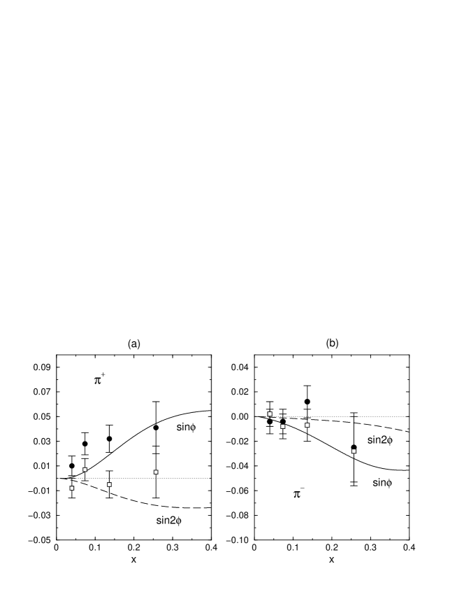
Fig.4 shows a preliminary comparison between the predictions of the CQSM and the HERMES experiments for the $\sin\phi$ and $\sin 2\phi$ asymmetries. The theoretical curves have been calculated as in [22],[23] by integrating over $y$ and $z$ in the HERMES kinematical range with the parameter $a=0.44\,\mbox{GeV}$ and $b=0.36\,\mbox{GeV}$ by assuming Gaussian distribution for the distribution functions and the fragmentation functions. The main difference with the similar analysis done in the same model [29] is that we have included all the subleading contributions into the distribution functions (no twist-2 approximation) as well as into the fragmentation functions. In fact, it turns out that the subleading term containing $\tilde{H}^{a}(z)$ in (11) gives sizable contributions to the $\sin\phi$ asymmetry. One can say that the theory reproduces the qualitative features of the data, although the uncertainties of the present experimental data are still too large to draw any decisive conclusion. As pointed out before, the HERMES group advocates that the observed small $\sin 2\phi$ asymmetry is consistent with the Ansatz $h_{1}(x)\simeq h_{L}(x)$, or equivalently $h_{1L}^{\perp(1)}(x)\simeq 0$. (Note that the formula for $\sin 2\phi$ asymmetry is proportional to this distribution function.) On the other hand, the CQSM as well as the MIT bag model indicates that these two functions are rather different especially in the small $x$ domain. Unfortunately, it seems difficult to draw a definite conclusion only from the present HERMES data for the $\sin 2\phi$ asymmetry. We certainly need more accurate experimental data.

From the theoretical viewpoint, the asymmetry obtained with a target polarized transversely to the direction of incident electron beam is much simpler [20]. Such asymmetry is proportional to

$$A^{\sin\phi}_{OT} \sim \frac{4\,\pi\alpha^{2}\,s}{Q^{4}}\,\,|S_{T}|\,\,(1-y)\,\,\sum_{a}\,\,e_{a}^{2}\,\,x\,h_{1}^{a}(x)\,\,H_{1}^{\perp(1)a}(z).$$ (21)

By measuring it, we can then get more direct information on the transversity distribution $h_{1}(x)$. Under the dominant-flavor-only approximation for the fragmentation functions, the semi-inclusive $\pi^{+}$ and $\pi^{-}$ productions respectively measure the following combinations of the transversity distributions :

$$\pi^{+}\ : \ \frac{4}{9}\,\,h_{1}^{u}(x)\ +\ \frac{1}{9}\,\,h_{1}^{\bar{d}}(x),$$ (22)

$$\pi^{-}\ : \ \frac{1}{9}\,\,h_{1}^{d}(x)\ +\ \frac{4}{9}\,\,h_{1}^{\bar{u}}(x).$$ (23)

Figure 5: Theoretical predictions for the combinations of the transversity distributions, $\frac{4}{9}h_{1}^{u}(x)+\frac{1}{9}h_{1}^{\bar{d}}(x)$ and $\frac{1}{9}h_{1}^{d}(x)+\frac{4}{9}h_{1}^{\bar{u}}(x)$ at $Q^{2}=2.5\,\mbox{GeV}^{2}$, which are to be measured in semi-inclusive $\pi^{+}$ and $\pi^{-}$ productions with a target proton polarized transversely to the direction of incident electron beam.

The solid curves in Fig. 5 stand for the full predictions of the CQSM for these distributions at $Q^{2}=2.5\,\mbox{GeV}^{2}$, while the dashed curves here are obtained by dropping the antiquark components in these combinations. One sees that the first combination is quite insensitive to the presence of the antiquark component, while the second one is sensitive to the antiquark component at least in the small $x$ region. This indicates that $\pi^{-}$ semi-inclusive production may be a useful tool to probe the role of antiquark in the transversity distributions.

In summary, we have given theoretical predictions for the chiral-odd distribution functions $h_{1}(x)$ and $h_{L}(x)$ within the framework of the CQSM, with full inclusion of the vacuum polarization effects as well as the subleading $1/N_{c}$ corrections. The importance of the vacuum polarization effects has been demonstrated by showing that the so-called Soffer inequality holds not only for the quark distributions but also for the antiquark ones. The theoretical predictions of the model for the azimuthal single spin asymmetries in the semi-inclusive electro-pion productions are shown to be qualitatively consistent with the corresponding HERMES data, although we certainly need more accurate experimental data as well as more precise knowledge about the T-odd fragmentation functions before drawing any decisive conclusion. We also find that the chiral-odd distribution functions have rather different magnitudes and $x$-dependencies as compared with the longitudinally polarized ones investigated in previous works. Especially interesting is that the transversity distribution have very small antiquark components. We hope that these unique predictions of the CQSM will be tested through near future semi-inclusive meaurements, which enables the flavor as well as the valence plus sea-quark decompositions.

Acknowledgement

The author would like to express his sincere thanks to K.A Oganessyan for useful discussion on the azimuthal single spin asymmetries in the semi-inclusive electro-pion productions.

References

- [1] R.L. Jaffe and X. Ji, Nucl. Phys. A375 (1992) 527.
- [2] J.C. Collins, Nucl. Phys. B396 (1993) 161.
- [3] HERMES Collaboration, A. Airapetian et al., Phys. Rev. Lett. 81 (2000) 4047.
- [4] D. Boer, hep-ph/9912311.
- [5] D.I. Diakonov, V.Yu. Petrov, and P.V. Pobylitsa, Nucl. Phys. B306, 809 (1988).
- [6] M. Wakamatsu and H. Yoshiki, Nucl. Phys. A524, 561 (1991).
- [7] M. Wakamatsu, Phys. Rev. D46 (1992) 3762.
-
[8]
D.I. Diakonov, V.Yu. Petrov, P.V. Pobylitsa,
M.V. Polyakov, and C. Weiss,
Nucl. Phys. B480, 341 (1996) ; ibid., Phys. Rev. D56, 4069 (1997). - [9] M. Wakamatsu and T. Kubota, Phys. Rev. D60, 034020 (1999).
[10]
EMC Collaboration, J. Aschman et al., Phys. Lett.
B206 (1988) 364 ;
Nucl. Phys. B328 (1989) 1. - [11] NMC Collaboration, P. Amaudruz et al., Phys. Rev. Lett. 66, 2712 (1991).
- [12] M. Wakamatsu and T. Watabe, Phys. Rev. D62 (2000) 017506.
- [13] B. Dressler, K. Goeke, M.V. Polyakov and C. Weiss, Eur. Phys. J. C14 (2000) 147.
- [14] T. Morii and T. Yamanishi, Phys. Rev. D61 (2000) 057501 ; M. Glück and E. Reya, Mod. Phys. Lett. A15 (2000) 883 ; D. de Florian and R. Sassot, Phys. Rev. D62 (2000) 094025 ; R.S. Bhalerao, hep-ph/0003075.
- [15] P.V. Pobylitsa and M.V. Polyakov, Phys. Lett. B389 (1996) 350.
- [16] L. Gamberg, H. Reinhardt and H. Weigel, Phys. Rev. D58 (1998) 054014.
[17]
M. Wakamatsu and T. Watabe, Phys. Lett. B312,
184 (1993) ;
Chr.V. Christov, A. Blotz, K. Goeke, P. Pobylitsa, V.Yu. Petrov, M. Wakamatsu,
and T. Watabe, Phys. Lett. B325, 467 (1994). - [18] J. Soffer, Phys. Rev. Lett. 74 (1995) 1292.
- [19] A. Kotzinian, Nucl. Phys. B441 (1995) 234.
- [20] R.D. Tangerman and P.J. Mulders, Phys. Rev. D51 (1995) 3357.
- [21] M. Boglione and P.J. Mulders, Phys. Lett. B478 (2000) 114.
- [22] K.A. Oganessyan, H.R. Avakian, N. Bianchi and A.M. Kotzinian, hep-ph/9808368 ; A.M. Kotzinian, K.A. Oganessyan, H.R. Avakian and E. De Sanctis, hep-ph/9908466.
- [23] K.A. Oganessyan, N. Bianchi, E. De Sanctis and W.-D. Nowak, hep-ph/0010261.
- [24] M. Glück, E. Reya and A. Vogt, Z. Phys. C67 (1995) 433.
- [25] M. Hirai, S. Kumano and M. Miyama, Comput. Phys. Commun. 111 (1998) 150.
- [26] I.I. Balitsky, V.M. Braun, Y. Koike and K. Tanaka, Phys. Rev. Lett. 77 (1996) 3078 ; A. Ali, V.M. Braun and G. Hiller, Phys. Lett. B266 (1991) 117.
- [27] Y. Kanazawa and Y. Koike, Phys. Lett. B403 (1997) 357.
- [28] M. Wakamatsu and T. Watabe, Phys. Rev. D62 (2000) 054009.
- [29] A.V. Efremov, K. Goeke, M.V. Polyakov and D. Urbano, Phys. Lett. B478 (2000) 94.