Abstract

Within the Standard Model, a review of the current determination of the sides and angles of the CKM unitarity triangle is presented, using experimental constraints from the measurements of $\left|\varepsilon_{K}\right|$, $\left|V_{ub}/V_{cb}\right|$, $\Delta m_{d}$ and from the limit on $\Delta m_{s}$, available in September 2000. Results from the experimental search for ${B}^{0}_{s}-\bar{{B}}^{0}_{s}$ oscillations are introduced in the present analysis using the likelihood. Special attention is devoted to the determination of the theoretical uncertainties. The purpose of the analysis is to infer regions where the parameters of interest lie with given probabilities. The BaBar “95% C.L. scanning” method is also commented.

To be submitted to JHEP

1 Introduction

In the Standard Model, weak interactions of quarks are governed by the four parameters of the CKM matrix [1] which, in the Wolfenstein parametrisation [2], are labelled as $\lambda,~{}A,~{}\bar{\rho}~{}{\rm and}~{}\bar{\eta}$ . Measurements of semileptonic decays of strange and beauty particles are the main sources of information on $\lambda$ and $A$, respectively. The values of $\left|\varepsilon_{K}\right|$, $\left|V_{ub}/V_{cb}\right|$, $\Delta m_{d}$ and ${\Delta m_{s}}$ provide a set of four constraints for $\bar{\rho}$ and $\bar{\eta}$. These constraints depend, in addition, on other quantities obtained from measurements and/or theoretical calculations. The regions of $\bar{\rho}$ and $\bar{\eta}$ preferred by the four constraints are expected to overlap, as long as the Standard Model gives an overall description of the various experimental observations.

Since several years there has been intense activity to constrain the allowed region in the ($\bar{\rho},\bar{\eta})$ plane from the best knowledge of the experimental and theoretical inputs [4]–[20]. Though the analysis methods differ in some details, they have a common ground in what we shall call standard approach through this paper. First, the goal of the various authors has been, explicitly or implicitly, to infer regions in which the values of $\bar{\rho}$ and $\bar{\eta}$ are contained with a certain level of probability (or confidence). Second, uncertainties due to statistical errors and systematic effects in experiments, as well as theoretical uncertainties, are combined together to deduce a global uncertainty about $\bar{\rho}$ and $\bar{\eta}$. As far as this second point is concerned, the various authors have used different “prescriptions” which can be seen, indeed, as approximations of the consistent Bayesian method which is described, and adopted, in this paper. The 68% probability regions favoured by the data and the theoretical understanding of the relevant processes select quite narrow regions for $\bar{\rho}$ and $\bar{\eta}$, largely independent of the details of the specific methods and of the different treatment of (experimental) systematic and theoretical uncertainties.

A different approach, named “95% C.L. scanning” in this paper, has been adopted in the BaBar Physics Book [23], and recently used in [24]. In this approach, it is stated that it is not possible to define probability distributions for theoretical parameters coming from calculations affected by systematic uncertainties or based on educated guesses (in practice all theoretical parameters and some experimental systematics belong to this class). On the basis of these considerations, the 95% C.L. scanning approach rejects the two basic points of the standard method and a different procedure is proposed. For the theoretical inputs, it is assumed that one can only define intervals inside which the true values of the parameters are contained. At fixed values of the theoretical inputs (within the allowed intervals) a maximum likelihood fit, which includes the other sources of uncertainties, is made, and 95% C.L. contours are determined. Finally, the envelope of such contours is “proposed to be a (conservative) method to obtain some 95% C.L. regions for all CKM parameters” [24]. Using the same arguments of the BaBar Physics Book [23], this procedure has been recently recommended in [25, 26], as opposed to the standard approach which is claimed of being too optimistic.

In view of the importance of constraining the parameters of the CKM matrix, or of the possibility of detecting signals of new physics in low-energy weak decays, in this paper we reconsider the whole matter, and in particular we focus on the most critical issues of the CKM-triangle analysis, namely the uncertainty on theoretical parameters and the inferential framework to handle consistently all uncertainties. This also allows to answer to several important controversial questions raised in the past, namely:

• whether it is possible, or necessary, to assign a probability distribution function (p.d.f.) to theoretical parameters;

• whether it is possible to define a p.d.f. for quantities extracted from physical measurements and from theoretical parameters affected by systematic uncertainties;

• whether average values, errors and p.d.f. of the quantities considered in the present analysis depend in a crucial way on the assumptions made on the theoretical parameters and the corresponding errors.

The main conclusions of this study are the following:

1. The standard method is a theoretically sound approach, which finds its justification within the inferential framework discussed in this paper. This method allows a consistent treatment of the systematic and theoretical uncertainties and makes it possible to define regions where the values of $\bar{\rho}$ and $\bar{\eta}$ (as well as of other quantities of phenomenological interest) are contained with any given level of confidence. In this respect the criticisms of [25, 26] are not justified.

2. The BaBar 95% C.L. scanning, instead, is based on an ad hoc prescription intended to define only a “95% C.L.” region. The meaning of this statement is unclear: the so called “95% C.L. region” does not correspond to the usual statistical definition of 95% confidence that the values of parameters lie in that region, neither in a frequentist sense, nor in a Bayesian one.

3. For the sake of comparison, with the standard method we have used the same values of the input parameters and tried to mimic the same uncertainties of the 95% C.L. scanning. We find that the “95% C.L.” regions selected in the $(\bar{\rho},~{}\bar{\eta})$ plane with the two methods are very similar, and it is thus not founded to qualify as too optimistic the standard approach.

4. In the 95% C.L. scanning approach the information contained in the p.d.f. of the relevant quantities ($\bar{\rho}$, $\bar{\eta}$, $\sin(2\beta)$, etc.) is missing. Thus we only know that a certain quantity is somehow expected in a given interval, but we do not know which is the most probable value, what is the shape of its p.d.f. etc. We show, instead, that this important information can be extracted from the data, using the standard method, in spite of the uncertainties in the theoretical parameters.

Regarding the analysis, since this kind of studies have been extensively illustrated in previous publications, see for example [14] and [19], here we only discuss in detail ${B}^{0}_{s}-\bar{{B}}^{0}_{s}$ mixing, for which we adopted a different procedure, based directly on the likelihood (Section 6).

The main results for the physical quantities ($\bar{\rho}$, $\bar{\eta}$, $\sin(2\beta)$, etc.) can be found in Sections 7.

The remainder of the paper is organised as follows. In Section 2 we summarise the theoretical constraints between $\bar{\rho}$ and $\bar{\eta}$ and the available experimental and theoretical inputs in the Standard Model. In Section 3 we describe the inferential framework used in this study and relate it to different standard approach analyses. Our comments on the 95% C.L. scanning method are also presented in this Section. The choice of values and uncertainties for the most critical theoretical parameters is discussed in Section 4. In Section 5 the p.d.f. determination for $\left|{V}_{cb}\right|$, $\left|{V}_{ub}\right|$ and the parameter $\lambda$ are explained. A new method to include the information coming from searches of ${B}^{0}_{s}-\bar{{B}}^{0}_{s}$ mixing is illustrated in Section 6. The results of the analysis are presented and discussed in Section 7. The stability of the results has been verified by varying the different input parameters in Section 8. A comparison of our results with those obtained with 95% C.L. scanning is made in Section 9. Finally, conclusions are drawn in Section 10.

2 Standard Model formulae relating $\bar{\rho}$ and $\bar{\eta}$ to experimental and theoretical inputs

Four measurements restrict, at present, the possible range of variations of the $\bar{\rho}$ and $\bar{\eta}$ parameters:

• The relative rate of charmed and charmless $b$-hadron semileptonic decays which allows to measure the ratio

  $$\left|\frac{V_{ub}}{V_{cb}}\right|=\frac{\lambda}{1~{}-~{}\frac{\lambda^{2}}{2}}\sqrt{\bar{\rho}^{2}+\bar{\eta}^{2}}\,.$$ (1)

  .

• The ${B}^{0}_{d}-\bar{{B}}^{0}_{d}$ time oscillation period which can be related to the mass difference between the light and heavy mass eigenstates of the ${B}^{0}_{d}-\bar{{B}}^{0}_{d}$ system

  $$\Delta m_{d}\ =\ {G_{F}^{2}\over 6\pi^{2}}m_{W}^{2}\ \eta_{c}S(x_{t})\ A^{2}\lambda^{6}\ [(1-\bar{\rho})^{2}+\bar{\eta}^{2}]\ m_{B_{d}}\ f_{B_{d}}^{2}\hat{B}_{B_{d}}\ ,$$ (2)

  where $S(x_{t})$ is the Inami-Lim function [27] and $x_{t}=m_{t}^{2}/M^{2}_{W}$. $m_{t}$ is the $\overline{MS}$ top mass, $m_{t}^{\overline{MS}}(m_{t}^{\overline{MS}})$, and $\eta_{c}$ is the perturbative QCD short-distance NLO correction. The remaining factor, $f_{B_{d}}^{2}\hat{B}_{B_{d}}$, encodes the information of non-perturbative QCD. Apart for $\bar{\rho}$ and $\bar{\eta}$, the most uncertain parameter in this expression is $f_{B_{d}}\sqrt{\hat{B}_{B_{d}}}$. The value of $\eta_{c}=0.55\pm 0.01$ has been obtained in [28] and we used $m_{t}=(167\pm 5)\,\rm{GeV}$, as deduced from measurements of the mass by CDF and D0 Collaborations [29].

• The limit on the lower value for the time oscillation period of the ${B}^{0}_{s}-\bar{{B}}^{0}_{s}$ system is transformed into a limit on $\Delta m_{s}$ and compared with $\Delta m_{d}$

  $$\frac{\Delta m_{d}}{\Delta m_{s}}~{}=~{}\frac{m_{B_{d}}f_{B_{d}}^{2}\hat{B}_{B_{d}}}{m_{B_{s}}f_{B_{s}}^{2}\hat{B}_{B_{s}}}\ \left(\frac{\lambda}{1-\frac{\lambda^{2}}{2}}\right)^{2}\ [(1-\bar{\rho})^{2}+\bar{\eta}^{2}]\,.$$ (3)

  The ratio $\xi~{}=~{}f_{B_{s}}\sqrt{\hat{B}_{B_{s}}}/f_{B_{d}}\sqrt{\hat{B}_{B_{d}}}$ is expected to be better determined from theory than the individual quantities entering into its expression. In our analysis, we accounted for the correlation due to the appearance of $\Delta m_{d}$ in both Equations (2) and (3).

• CP violation in the kaon system which is expressed by $\left|\varepsilon_{K}\right|$

  $$\left|\varepsilon_{K}\right|\ =C_{\varepsilon}\ A^{2}\lambda^{6}\ \bar{\eta}\left[-\eta_{1}S(x_{c})+\eta_{2}S(x_{t})\left(A^{2}\lambda^{4}\left(1-\bar{\rho}\right)\right)+\eta_{3}S(x_{c},x_{t})\right]\ \hat{B}_{K}\ ,$$ (4)

  where

  $$C_{\varepsilon}=\frac{G_{F}^{2}f_{K}^{2}m_{K}m_{W}^{2}}{6\sqrt{2}\pi^{2}\Delta m_{K}}\ .$$ (5)

  $S(x_{i})$ and $S(x_{i},x_{j})$ are the appropriate Inami-Lim functions [27] of $x_{q}=m_{q}^{2}/m_{W}^{2}$, including the next-to-leading order QCD corrections [28, 30]. The most uncertain parameter is $\hat{B}_{K}$.

Constraints are obtained by comparing present measurements with theoretical expectations using the expressions given above and taking into account the different sources of uncertainties. In addition to $\bar{\rho}$ and $\bar{\eta}$, these expressions depend on other quantities which have been listed in Table 1. Additional measurements or theoretical determinations have been used to provide information on the values of these parameters.

Parameter	Value	Gaussian	Uniform	Ref.
		$\sigma$	half-width
$\lambda$	$0.2237$	$0.0033$ , see text		sect. 5.3 (eq. 46)
$\left|V_{cb}\right|$	$41.0\times 10^{-3}$	$1.6\times 10^{-3}$ , see text		sect. 5.1 (eq. 43)
$\left|V_{ub}\right|$	$35.5\times 10^{-4}$	$3.6\times 10^{-4}$	–	sect. 5.2 (eq. 45)
$\left|\varepsilon_{K}\right|$	$2.271\times 10^{-3}$	$0.017\times 10^{-3}$	–	[31]
$\Delta m_{d}$	$0.487~{}\mbox{ps}^{-1}$	$0.014~{}\mbox{ps}^{-1}$	–	[32]
$\Delta m_{s}$	$>$ 15.0 ps-1 at 95% C.L.	see text		[32]
$m_{t}$	$167~{}\rm{GeV}$	$5~{}\rm{GeV}$	–	[29]
$m_{b}$	$4.23~{}\rm{GeV}$	$0.07~{}\rm{GeV}$	–	[33]
$m_{c}$	$1.3~{}\rm{GeV}$	$0.1~{}\rm{GeV}$	–	[31]
$\hat{B}_{K}$	$0.87$	$0.06$	$0.13$	sect. 4 (eq. 34)
$f_{B_{d}}\sqrt{\hat{B}_{B_{d}}}$	$230~{}\rm MeV$	$25~{}\rm MeV$	$20~{}\rm MeV$	sect. 4 (eq. 28)
$\xi=\frac{f_{B_{s}}\sqrt{\hat{B}_{B_{s}}}}{f_{B_{d}}\sqrt{\hat{B}_{B_{d}}}}$	$1.14$	0.04	$0.05$	sect. 4 (eq. 31)
$\alpha_{s}$	$0.119$	$0.03$	–	[30]
$\eta_{1}$	$1.38$	$0.53$	–	[30]
$\eta_{2}$	$0.574$	$0.004$	–	[28]
$\eta_{3}$	$0.47$	$0.04$	–	[30]
$\eta_{b}$	$0.55$	$0.01$	–	[28]
$f_{K}$	$0.159~{}\rm{GeV}$	fixed		[31]
$\Delta m_{K}$	$0.5301\times 10^{-2}~{}\mbox{ps}^{-1}$	fixed		[31]
$G_{F}$	$1.16639\times 10^{-5}\rm{GeV}^{-2}$	fixed		[31]
$m_{W}$	$80.42~{}\rm{GeV}$	fixed		[31]
$m_{B^{0}_{d}}$	$5.2792~{}\rm{GeV}$	fixed		[31]
$m_{B^{0}_{s}}$	$5.3693~{}\rm{GeV}$	fixed		[31]
$m_{K}$	$0.493677~{}\rm{GeV}$	fixed		[31]

Table 1: Values of the quantities entering into the expressions of $\left|\varepsilon_{K}\right|$, $\left|V_{ub}/V_{cb}\right|$, $\Delta m_{d}$ and $\Delta m_{s}$. In the third and fourth columns the Gaussian and the flat part of the uncertainty are given, respectively.

3 Inferential framework

In this Section we recall the basic ingredients of the standard method, interpreted in the framework of the Bayesian approach. This allows us to discuss the role of the systematic and theoretical uncertainties in deriving probability intervals for the relevant parameters.

3.1 Standard approach and Bayesian inference

Each of Equations (1)–(4) relates a constraint $c_{j}$ (where $c_{j}$ stands for $\left|V_{ub}/V_{cb}\right|$, $\Delta m_{d}$, $\Delta m_{d}/\Delta m_{s}$ and $\left|\varepsilon_{K}\right|$, for $j=1,\ldots,4$) to the CKM–triangle parameters $\bar{\rho}$ and $\bar{\eta}$, via the set of ancillary parameters ${\mathbf{x}}$, where ${\mathbf{x}}=\{x_{1},x_{2},\ldots,x_{N}\}$ stand for all experimentally determined or theoretically calculated quantities from which the various $c_{j}$ depend

$$c_{j}=c_{j}(\bar{\rho},\bar{\eta};{\mathbf{x}}).$$ (6)

In an ideal case of exact knowledge of $c_{j}$ and ${\mathbf{x}}$, each of the constraints provides a curve in the $(\bar{\rho},\bar{\eta})$ plane. In such a case, there would be no reason to favour any of the points on the curve, unless we have some further information or physical prejudice, which might exclude points outside a determined physical region, or, in general, assign different weights to different points. In a realistic case, we suffer from several uncertainties on the quantities $c_{j}$ and ${\mathbf{x}}$. Uncertainty does not imply, however, that we are absolutely ignorant about a given quantity. First of all, there are values which, to the best of our knowledge, we consider ruled out (for example a value of $m_{t}$ of 100 GeV or 500 GeV). Second, we assign different probabilities to the values within the “almost certain range”, $147\,\mbox{GeV}<m_{t}<187\,\mbox{GeV}$ say . In the $m_{t}$ case, for example, we think that it is much more probable that the value of ${m}_{t}$ lies between 157 and 177 GeV rather than in the rest of the interval, in spite of the fact that the two sub-intervals have the same widths.

This means that, instead of a single curve (6) in the $(\bar{\rho},\bar{\eta})$ plane, we have a family of curves which depends on the distribution of the set $\{c_{j},{\mathbf{x}}\}$. As a result, the points in the $(\bar{\rho},\bar{\eta})$ plane get different weights (even if they were taken to be equally probable a priori) and our confidence on the values of $\bar{\rho}$ and $\bar{\eta}$ clusters in a region of the plane.

The above arguments, which we consider very natural and close to physicist intuition, can be formalised by using the so called Bayesian approach (see [34] for an introduction). In this approach, the uncertainty is described in terms of a probability density function $f(\cdot)$, which quantifies our confidence on the values of a given quantity. The inference of $\bar{\rho}$ and $\bar{\eta}$ becomes then a straightforward application of probability theory, getting rid of all “ad hoc prescriptions”.

The simplest way to implement the probabilistic reasoning discussed above is to define an idealised “p.d.f.” for each constraint

$$f(\bar{\rho},\bar{\eta}\,|\,c_{j},{\mathbf{x}})\propto\delta(c_{j}-c_{j}(\bar{\rho},\bar{\eta},{\mathbf{x}}))\,,$$ (7)

where $\delta$ is the Dirac delta distribution. The quotes recall us that this p.d.f. is a distribution in a mathematical sense, which is to be taken as the limit of a very narrow p.d.f. with values different from zero only along a curve. The p.d.f. which takes into account the full uncertainty about $c_{j}$ and ${\mathbf{x}}$ is obtained from (7) by making use of the standard probability rules

$$f(\bar{\rho},\bar{\eta}) = \int f(\bar{\rho},\bar{\eta}\,|\,c_{j},{\mathbf{x}})\cdot f(c_{j},{\mathbf{x}})\,\mbox{d}c_{j}\,\mbox{d}{\mathbf{x}}$$ (8)

$$\propto \int\delta(c_{j}-c_{j}(\bar{\rho},\bar{\eta},{\mathbf{x}}))\cdot f(c_{j})\cdot f({\mathbf{x}})\,\mbox{d}c_{j}\,\mbox{d}{\mathbf{x}}$$ (9)

$$\propto \int\delta(c_{j}-c_{j}(\bar{\rho},\bar{\eta},{\mathbf{x}}))\cdot\frac{1}{\sqrt{2\pi}\,\sigma(c_{j})}\exp\left[-\frac{(c_{j}-\hat{c}_{j})^{2}}{2\,\sigma^{2}(c_{j})}\right]\cdot f({\mathbf{x}})\,\mbox{d}c_{j}\,\mbox{d}{\mathbf{x}}$$ (10)

$$\propto \int\frac{1}{\sqrt{2\pi}\,\sigma(c_{j})}\exp\left[-\frac{(c_{j}(\bar{\rho},\bar{\eta},{\mathbf{x}})-\hat{c}_{j})^{2}}{2\,\sigma^{2}(c_{j})}\right]f(x_{1})\cdot f(x_{2})\cdots f(x_{N})\,\mbox{d}{\mathbf{x}}\,,$$ (11)

where $\hat{c}_{j}$ is the experimental best estimate of $c_{j}$, with uncertainty $\sigma(c_{j})$. A Gaussian distribution has been assumed just for simplicity and without lack of generality. The joint p.d.f. $f(c_{j},{\mathbf{x}})$ has been splitted as a product of the individual p.d.f., assuming the independence of the different quantities, which is a very good approximation for the case under study.

As alternative procedure, one may introduce a global inference relating $\bar{\rho}$, $\bar{\eta}$, $c_{j}$ and ${\mathbf{x}}$. This is followed by a second step where marginalization is performed over those quantities which we are not interested to. In this case, by making use of Bayes’ theorem, we obtain

$$f(\bar{\rho},\bar{\eta},c_{j},{\mathbf{x}}\,|\,\hat{c}_{j}) \propto f(\hat{c}_{j}\,|\,c_{j},\bar{\rho},\bar{\eta},{\mathbf{x}})\cdot f(c_{j},\bar{\rho},\bar{\eta},{\mathbf{x}})$$ (12)

$$\propto f(\hat{c}_{j}\,|\,c_{j})\cdot f(c_{j}\,|\,\bar{\rho},\bar{\eta},{\mathbf{x}})\cdot f({\mathbf{x}},\bar{\rho},\bar{\eta})$$ (13)

$$\propto f(\hat{c}_{j}\,|\,c_{j})\cdot\delta(c_{j}-c_{j}(\bar{\rho},\bar{\eta},{\mathbf{x}}))\cdot f({\mathbf{x}})\cdot f_{\circ}(\bar{\rho},\bar{\eta})\,,$$ (14)

where $f_{\circ}(\bar{\rho},\bar{\eta})$ denotes the prior distribution as often used in the literature. The various steps follow from probability rules, by assuming the independence of the different quantities and by noting that $\hat{c}_{j}$ depends on ($\bar{\rho},\bar{\eta},{\mathbf{x}}$) only via $c_{j}$. This is true since $c_{j}$ is univocally determined, within the Standard Model, from the values of $\bar{\rho}$, $\bar{\eta}$ and ${\mathbf{x}}$ (hence the limit to a delta function of its p.d.f.). We then recover Equation (11): i) by assuming a Gaussian error function for $\hat{c}_{j}$ around $c_{j}$; ii) by considering the various $x_{i}$ as independent; iii) by taking a flat a priori distribution for $\bar{\rho}$ and $\bar{\eta}$ and iv) by integrating Equation (14) over $c_{j}$ and ${\mathbf{x}}$. Note that equiprobability of all points in the $(\bar{\rho},\bar{\eta})$ plane was also implicit in Equation (9), as discussed above.

Although the first derivation of Equation (9) is probably the most intuitive one, hereafter we use the second one, which is the usual way of performing Bayesian inference. The second procedure also shows explicitly the connection with the methods which we denoted as standard in the introduction.

The extension of the formalism to several constraints is straightforward. We can rewrite Equation (12) as

$$f(\bar{\rho},\bar{\eta},{\mathbf{x}}\,|\,\hat{c}_{1},...,\hat{c}_{\rm M}) \propto \prod_{j=1,{\rm M}}f_{j}(\hat{c}_{j}\,|\,\bar{\rho},\bar{\eta},{\mathbf{x}})\times\prod_{i=1,{\rm N}}f_{i}(x_{i})\times f_{\circ}(\bar{\rho},\bar{\eta})\ .$$ (15)

In the derivation of (15), we have used the independence of the different quantities. Moreover, the conditioning from $f_{j}(\cdot)$ on the $c_{j}$ have been removed, since the $c_{j}$ act as intermediate variables which are finally integrated away. The derivation (8)–(11) can also be easily extended to the case of several constraints and leads, again, to the same result as that found by using Bayes’ theorem. We have only to account properly the weight on $c_{j}$, induced by the other constraint(s) previously considered. In this case Equation (7) becomes $f(\bar{\rho},\bar{\eta}\,|\,c_{1},\dots,c_{M},{\mathbf{x}})\propto\delta(c_{M}-c_{M}(\rho,\eta,{\mathbf{x}}))\cdot f(\rho,\eta\,|\,c_{1},\dots,c_{M-1},{\mathbf{x}})$.

By integrating Equation (15) over ${\mathbf{x}}$ we can rewrite the inferential scheme in the following convenient way

$$f(\bar{\rho},\bar{\eta}\,|\,{\mathbf{\hat{}}{c}},{\mathbf{f}})\propto{\cal L}({\mathbf{\hat{}}{c}}\,|\,\bar{\rho},\bar{\eta},{\mathbf{f}})\times f_{\circ}(\bar{\rho},\bar{\eta})\,,$$ (16)

where ${\mathbf{\hat{}}{c}}$ stands for the set of measured constraints, and

$${\cal L}({\mathbf{\hat{}}{c}}\,|\,\bar{\rho},\bar{\eta},{\mathbf{f}})=\int\prod_{j=1,{\rm M}}f_{j}(\hat{c}_{j}\,|\,\bar{\rho},\bar{\eta},{\mathbf{x}})\prod_{i=1,{\rm N}}f_{i}(x_{i})\,\mbox{d}{x_{i}}$$ (17)

is the effective overall likelihood which takes into account all possible values of $x_{j}$, properly weighted. We have written explicitly that the overall likelihood depends on the best knowledge of all $x_{i}$, described by $f({\mathbf{x}})$.

Whereas a priori all values for $\bar{\rho}$ and $\bar{\eta}$ are considered equally likely, a posteriori the probability clusters around the point which maximises the likelihood. This is the reason why, in principle, different procedures for determining $\bar{\rho}$ and $\bar{\eta}$, based on the maximum likelihood, are equivalent to the method described here and should get similar results. We say “in principle” because other methods are typically implemented using the $\chi^{2}$ minimisation. This implies the assumption of a multi-Gaussian solution of the integral (17), with overall standard deviations which are simply a quadratic combinations of the “uncertainties” related to each $x_{i}$. On the other hand, a quadratic combination relies on the approximative linear dependence of $c_{j}$ from the possible variations of $x_{i}$.

In conclusion, the final (unnormalised) p.d.f. obtained starting from a flat distribution of $\bar{\rho}$ and $\bar{\eta}$ is

$$f(\bar{\rho},\bar{\eta})\propto\int\prod_{j=1,{\rm M}}f_{j}(\hat{c}_{j}\,|\,\bar{\rho},\bar{\eta},{\mathbf{x}})\prod_{i=1,{\rm N}}f_{i}(x_{i})\,\mbox{d}{x_{i}}\,.$$ (18)

The integration can be done by Monte Carlo methods, the normalisation is trivial, and all moments can be calculated in a (conceptually) easy way. Obviously there are several ways to implement the Monte Carlo integration, using different techniques to generate events. A comparison of the results obtained with the approach of [19], where some effort has been done to improve the generation efficiency, and the results of [14] is presented in Section 7.

It is important to note that the inferential method does not make any distinction on whether the individual likelihood associated to some constraint is different from zero only in a narrow region (and we usually refer to this case as “measurement”), or it goes to zero only on one of the two sides (e.g. when $c_{j}\rightarrow\infty$ or $0$). In the latter case, the data only provide an upper/lower bound to the value of the constraint. This is precisely what happens, at present, with $\Delta m_{s}$. Therefore, the experimental information about this constraint enters naturally in the analysis (more details can be found in Section 6).

3.2 Treatment of systematic and theoretical uncertainties

At this point, it is in order a discussion on some important ingredients of the analysis which raised some controversy in the past. They are related to the quantitative handling of the uncertainties due to systematic effects and to theoretical inputs.

In Equation (9) we have written explicitly that $\hat{c}_{j}$ is Gaussian distributed around $c_{j}$. As a consequence, we tend to say that also $c_{j}$ is Gaussian distributed around $\hat{c}_{j}$, the inversion being well understood in the case of random errors. The question is how to include the case where also systematic uncertainties are present. One of the nice features of the Bayesian approach is that the uncertainty has positively the same meaning, and there is no conceptual distinction between the uncertainty due to random fluctuations, which might have occurred in the measuring process, the uncertainty about the parameters of the theory, and the uncertainty about influence quantities (i.e. “systematics”) of not-exactly-known value, (see [34] and [35]). Under the assumption that the individual likelihoods $f_{j}(\cdot)$ of Equations (15)–(18) do only depend on random effects, the uncertainty due to systematics can be included using, again, concepts and formulae of conditional probability. In fact, calling ${\mathbf{h}}$ the set of influence quantities on which the measured constraints may depend, with joint p.d.f. $g({\mathbf{h}})$, the likelihood (17) becomes

$${\cal L}({\mathbf{\hat{}}{c}}\,|\,\bar{\rho},\bar{\eta},{\mathbf{f}},{\mathbf{g}})=\int\prod_{j=1,{\rm M}}f_{j}(\hat{c}_{j}\,|\,\bar{\rho},\bar{\eta},{\mathbf{x}},{\mathbf{h}})\cdot f({\mathbf{x}})\cdot g({\mathbf{h}})\,\mbox{d}{\mathbf{x}}\,\mbox{d}{\mathbf{h}}\,,$$ (19)

where we have written the p.d.f. of ${\mathbf{x}}$ in its general form, allowing also correlations among the elements. As can be seen from Equation (19), there is neither a conceptual nor a formal distinction between the handling of ${\mathbf{x}}$ and ${\mathbf{h}}$. Therefore, we can simply extend the notation to include in ${\mathbf{x}}$ the influence parameters responsible of the systematic uncertainty, and use Equation (17) in an extended way. This is what it has been actually done in the past to infer $f(\bar{\rho},\bar{\eta})$ with the Monte Carlo integration method resulting from (18). Moreover, see also [35] and references therein, we arrive to the following conclusion. Irrespectively of the assumptions made on the p.d.f. of ${\mathbf{x}}$, the overall likelihoods $f(\hat{c}_{j})$ are approximately Gaussian because of a mechanism similar to the central limit theorem (i.e. just a matter of combinatorics). This makes the results largely stable against variations within reasonable choices of models and parameters used to describe the uncertainties due to theory and systematics. This also explains why methods based on $\chi^{2}$ minimisation (for example refs. [16], [17] and [18]) can be considered as approximations of the one used in refs. [13],[14], [15] and [19]. We stress again that a common ground of all the methods that we classify as standard is to produce regions where $\bar{\rho}$ and $\bar{\eta}$ are contained with any given level of confidence. On the contrary, the BaBar 95% C.L. scanning is based on an ad hoc prescription which obscures the meaning of the results. In that approach, a so called “95% C.L.” is produced, which does not correspond to the usual 95% confidence that the parameters lie in that regions.

As far as the choice of the mathematical expression for $f_{i}(x_{i})$ is concerned, practical examples of simple models can be found in  [35]. Due to the insensitivity of the result on the precise model, as discussed previously and as shown later in this paper, we simplify the problem, by reducing the choice only to two possibilities. We choose a Gaussian model when the uncertainty is dominated by statistical effects, or there are many comparable contributions to the systematics error, so that the central limit theorem applies. We choose a uniform p.d.f. if the parameter is believed to be (almost) certainly in a given interval, and the points inside this interval are considered equally probable.

A final comment, before ending this Section, concerns the compatibility among inferences provided by individual constraints. In the simplified approach based on $\chi^{2}$ minimisation, a conventional evaluation of compatibility stems automatically from the value of the $\chi^{2}$ at its minimum. This information is lost in the likelihood approach, but we accept this loss without any regret, in view of what we gain. It is well known, indeed, that crude arguments about compatibility or incompatibility, based only on the minimum value of the $\chi^{2}$ and the number of degrees of freedom lead to misleading conclusions (as premature claims of new physics have demonstrated in the past decades). Therefore, we consider more reasonable to judge the compatibility of the constraints by comparing partial inferences obtained when removing each constraint at the time. Examples are given in Figures 9 and 11. In our analysis, the overlap of the various constraints is excellent, and therefore we have no reason to suspect deviations from the Standard Model, given the available experimental information.

4 Theoretical inputs: $B_{K}$, $f_{B}\sqrt{\hat{B}_{B}}$ and the $\xi$ parameter

In this Section we discuss the theoretical inputs which have been used in our phenomenological analysis. In particular, we explain how central values and uncertainty models for the different quantities have been chosen. This gives us the opportunity of clarifying some issues on which there is, we think, some confusion in the literature. This discussion may be instructive especially for non-lattice experts (often experimentalists) who are engaged in this kind of analyses and have to find some orientation in using results from a plethora of lattice studies.

For example, in ref. [20], the renormalization-scheme dependence of the meson decay constants is mentioned. Unfortunately decay constants (which are related to matrix elements of the weak axial current), as all measurable physical quantities, are scheme independent by definition. Indeed the physical, scheme-independent axial current is obtained from the lattice one by a finite renormalization constant, $A_{\mu}=Z_{A}A_{\mu}^{latt}$, which can be (has been) determined non-pertubatively with a negligible uncertainty [36, 37]. Scheme dependence only enters some theoretical predictions (but never in those for the decay constants) because the perturbative calculations of the Wilson coefficients in the effective Hamiltonians, relevant for weak decays and mixing, are truncated at a certain order (typically NLO). This is not a peculiarity of the lattice approach but it depends on the limited number of orders which has been computed in continuum perturbation theory. Moreover, the choice of presenting the calculations in $\overline{MS}$ is only a traditional option which has not to do with the continuum or the lattice formulation of the theory. A discussion of this point in the case of $B^{0}$–$\bar{B}^{0}$ mixing can be found below.

Another source of confusion is the uncontrolled propagation of values and errors of the parameters from one review talk to another, without verification on the original papers, and regardless of more recent calculations and progresses. A typical example is the value $\xi\sim 1.3$. This number was only found in [38]. All other lattice calculations find for this quantity values between $1.11$ and $1.17$ [39]–[42] in the quenched approximation and similar numbers have been recently confirmed by unquenched data [42]. Similarly, in [25], A. Falk quotes $\xi=1.14(0.13)$ on the basis of a two-year old review by S. Sharpe [43]. In the absence of unquenched calculations, the rather generous uncertainty reported in [43] was justified, at the time, on the basis of theoretical estimates obtained by using quenched and unquenched chiral perturbation theory. These estimates have not been confirmed by (partially) unquenched results, which were already available last year . Irrespectively of recent lattice progresses, this very large uncertainty, which is not supported by any explicit numerical result, risks to survive and be used in future phenomenological analyses. The most recent figures for the $B$-meson decay constants, the $B$-parameters, $f_{B_{d}}\sqrt{\hat{B}_{B_{d}}}$ and $\xi$ can be found in Tables 2 and 3. These tables include the results presented at Lattice 2000 [42]. In the following, for all the theoretical parameters, we have used results taken from lattice QCD. There are several reasons for this choice, which has been adopted also in previous studies of the unitarity triangle [5, 8, 13, 14, 19]. Lattice QCD is not a model, as the quark model for example, and therefore physical quantities can be computed from first principles without arbitrary assumptions. It provides a method for predicting all physical quantities (decay constants, weak amplitudes, form factors) within a unique, coherent theoretical framework. For many quantities the statistical errors have been reduced to the percent level (or even less). Although most of the results are affected by systematic effects, the latter can be “systematically” studied and eventually corrected. All the recent literature on lattice calculations is indeed focused on discussions of the systematic errors and studies intended to reduce these sources of uncertainty. We are not aware of any other approach (1/N expansion, QCD Sum Rules, etc.) where such a deep investigation of systematic errors is being carried out for a so large set of physical quantities as in lattice QCD. Finally, in cases where predictions (non post-dictions) from lattice QCD have been compared with experiments, for example $f_{D_{s}}$, the agreement has been found very good.

Obviously, for some quantities the uncertainty from lattice simulations is far from being satisfactory and further effort is needed to improve the situation. For the quantities considered here this is particularly true for the ${B}^{0}_{d}$–$\bar{B}^{0}_{d}$ mixing amplitude, as discussed below. Nevertheless, for the reasons mentioned before, we think that lattice results and uncertainties are the most reliable ones and we have used them in our study.

4.1 Statistical and systematic effects in lattice calculation uncertainties

Lattice simulations are theoretical experiments carried out by numerical integration of the functional integral by Monte Carlo techniques. In this respect uncertainties are evaluated following criteria very close to those used in experimental measurements. The results are obtained with “statistical errors”, i.e. uncertainties originated by stochastic fluctuations, which may be reduced by increasing the sample of gluon-field configurations on which the averages are performed. It is very reasonable to assume that the statistical fluctuations have a Gaussian (almost Gaussian) distribution. Hence, the probabilistic inversion needed to infer the quantity of interest gives rise to Gaussian uncertainty models.

To convert the results of lattice simulations in predictions for the physical amplitudes several steps are necessary:

• renormalization of the relevant operators;

• extrapolation to the continuum limit, namely to zero lattice spacing ($a\to 0$);

• unquenched calculations. The most precise numbers have been obtained in the quenched approximation. Theoretical estimates and some preliminary results in the (partially) unquenched case are also known and they are used to estimate the systematic errors of the quenched results.

a)–c) are the main sources of systematic errors for $B_{K}$, $f_{B_{q}}\sqrt{\hat{B}_{B_{q}}}$ and $\xi$ and are discussed separately in the following. Here we want only to stress that systematic errors from lattice calculations are conceptually similar to some of the systematic errors present in experimental measurements.

Let us consider as an example discretization errors. Since it is obviously impossible to work at zero lattice spacing, a method to correct for discretization effects is to compute a given physical quantity at different values of the lattice spacing and to extrapolate it to zero lattice spacing. The theory tells us whether the extrapolation has to be linear or quadratic in $a$. Thus for example one fits a given quantity $Q$ as

$$Q(a)=Q(a=0)+Q^{\prime}a+Q^{\prime\prime}a^{2}+\ldots\,,$$ (20)

and takes $Q(a=0)$ as best estimate of the value of $Q$ in the continuum limit. Since the “measurements” performed at fixed lattice spacing are subject to a statistical error, the uncertainty in the extrapolated quantity is inflated with respect to the points directly measured. In the quenched case, extrapolations have been made for both $\hat{B}_{K}$, the $B$-meson decay constants and $\xi$. Systematic studies for the $B$-meson mixing parameters are still missing. From a comparison among calculations performed by different groups at different lattice spacing and with different lattice actions, an estimate of discretization errors can be obtained, however, also in these cases.

When an extrapolation to the continuum limit of the lattice data has been possible, the final uncertainty results from the statistical error of the points measured at fixed lattice spacing (a residual uncertainty is present when linear or linear plus quadratic extrapolations give different results). Thus, in this case, it is natural to assume that the final error has a Gaussian distribution.

As for the errors coming from quenched calculations, partially unquenched calculations exist for several quantities considered in this study, namely $\hat{B}_{K}$ and $f_{B_{d,s}}$. These calculations are usually performed with two light quarks in the fermion loops, at values of the light-quark masses larger than the physical values and an extrapolation in these masses is required. The calculations are generally made at a fixed value of the lattice spacing and thus contain discretization errors. An estimate of the quenching errors is obtained by comparing quenched and unquenched results at similar values of the lattice spacing. These comparisons are complemented by theoretical estimates of this uncertainty obtained by using quenched and unquenched chiral perturbation theory techniques [44].

The question arising at this point is: what is the best model to describe the theoretical systematic errors in lattice calculations, and hence the assessment of the uncertainty? We refer to the general introduction of the inferential framework given in Section 3. As happens with systematic errors in experiments, this completely relies on the confidence of the experts about possible variations of an influence parameter, the effect of quenching or what would happen in passing from a perturbative order to the other or changing the renormalization scheme. These evaluations are unavoidably subjective, though not arbitrary, as long as we use the judgements of responsible experts for each input quantity. Using their judgements we commit ourselves too. Therefore, hereafter, when we state that a parameter lies in a certain range with uniform distribution, it means that, in practice, we are 100% confident that the parameter lies in that region, and that, for any choice of a sub-interval of half the width, we are in condition of indifference (i.e. 50% confidence) that the value of the parameter is inside the sub-interval or somewhere else. For a more extended discussion see for example [45] and references therein.

In conclusion, we cannot find any conceptual difference which would force us to treat experimental and theoretical uncertainties on a different footing and claim that the standard method is a perfectly justified scientific approach able to establish confidence levels for the quantities of interest. In the following, for each parameter, taken from lattice QCD evaluations, best estimates for its central value and attached uncertainties are given.

In order to check the stability of the results, we have also made the analysis with the flat part of the theoretical uncertainty increased by a factor two.

4.2 Evaluation of the parameter $f_{B_{d}}\sqrt{\hat{B}_{B_{d}}}$

Traditionally, the $B$-parameter of the renormalized operator is defined as

$$\langle\bar{B}_{d}|Q_{d}^{\Delta B=2}(\mu)|{B}_{d}\rangle=\frac{8}{3}\ m_{B_{d}}^{2}f_{B_{d}}^{2}\ B_{B_{d}}(\mu)\,,$$ (21)

where $Q_{d}^{\Delta B=2}=(\bar{b}\gamma^{\mu}(1-\gamma_{5})d)(\bar{b}\gamma_{\mu}(1-\gamma_{5})d)$ and $\mu$ is the renormalization scale. This definition stems from the vacuum saturation approximation (VSA) in which $B_{B_{d}}=1$. Similarly one can define $B_{B_{s}}$. The renormalization group invariant $B$-parameter $\hat{B}_{B_{d}}$ of Equation (2) is defined as

$$\hat{B}_{B_{d}}=\alpha_{s}(\mu)^{-\gamma_{0}/2\beta_{0}}\left(1+{\alpha_{s}(\mu)\over 4\pi}J\right)\ B_{B_{d}}(\mu)\ .$$ (22)

$\gamma_{0}=4$ in all schemes whereas $J$ depends on the scheme used for renormalizing $Q_{d}^{\Delta B=2}(\mu)$. In the theoretical expressions, the physical amplitudes are always defined in terms of $\hat{B}_{B_{d}}$. The advantage is that this quantity is not only renormalization scale, but also renormalization-scheme independent. A residual scheme dependence remains only because the coefficient renormalizing the lattice operator is computed at a fixed order in perturbation theory (NLO in this case), whereas its matrix element is computed non-perturbatively. This problem would arise in any approach that computes physical amplitudes by combining the Wilson coefficients of the effective Hamiltonian, which are computed perturbatively, with hadronic matrix elements. Thus it is not specific to lattice calculations. The scheme dependence can be reduced by increasing the order at which Wilson coefficients are computed in continuum perturbation theory.

Indeed the important quantity is not the $B$-parameter itself but the combination $(f_{B_{d}}\sqrt{\hat{B}_{B_{d}}})^{2}$ which is used as an alias for the physical amplitude to which it is simply related by the factor $8m_{B_{d}}^{2}/3$. This is similar to the kaon $B$ parameter. In that case, however, the decay constant is taken from experiments. For the ${B}_{d}$ meson, instead, we have to rely on theory also for the decay constant. Since the calculation of $f_{B_{d}}$ and $\hat{B}_{B_{d}}$ are strongly correlated, the best way is to take the combination $f_{B_{d}}\sqrt{\hat{B}_{B_{d}}}$ from a single calculation rather than using $f_{B_{d}}$ and $\hat{B}_{B_{d}}$ from different studies as often done in the literature.

The most recent calculations of the combination $f_{B_{d}}\sqrt{\hat{B}_{B_{d}}}$, in the quenching approximation, come from ref. [51], obtained with the non-perturbatively improved action and a non-perturbative renormalization of the lattice operators, and from ref. [55], with the mean-field improved action and perturbatively renormalized operators

$$f_{B_{d}}\sqrt{\hat{B}_{B_{d}}} = (206\pm 28\pm 7)\,{\rm MeV}\quad\cite[cite]{[\@@bibref{}{ape00}{}{}]}\,,$$

$$f_{B_{d}}\sqrt{\hat{B}_{B_{d}}} = (211\pm 21^{+27}_{-28})\,{\rm MeV}\quad\cite[cite]{[\@@bibref{}{ll2000}{}{}]}\,.$$ (23)

These results correspond to the following values obtained in the same simulation

$$f_{B_{d}} = (174\pm 22^{+7+4}_{-0-0})\,{\rm MeV}\,\quad\hat{B}_{B_{d}}=1.38\pm 0.11^{+0.00}_{-0.09}\quad\cite[cite]{[\@@bibref{}{ape00}{}{}]}\,,$$

$$f_{B_{d}} = (177\pm 17^{+22}_{-26})\,{\rm MeV}\,\quad\hat{B}_{B_{d}}=1.41\pm 0.06^{+0.05}_{-0.01}\quad\cite[cite]{[\@@bibref{}{ll2000}{}{}]}\,.$$ (24)

Quenched		$f_{B_{d}}$ (MeV)	$f_{B_{s}}/f_{B_{d}}$	$f_{D}$ (MeV)	$f_{D_{s}}$ (MeV)
APE [46]	97	$180(32)$	$1.14(8)$	$221(17)$	$237(16)$
FNAL [47]	97	$164(^{+14}_{-11})(8)$	$1.13(^{+5}_{-4})$	$194(^{+14}_{-10})(10)$	$213(^{+14}_{-11})(11)$
JLQCD [48]	98	$173(4)(12)$	$\simeq 1.15$	$197(2)(17)$	$224(2)(19)$
MILC(∗) [49]	98	$157(11)(^{+25}_{-9})(^{+23}_{-0})$	$1.11(2)(^{+4}_{-3})(3)$	$192(11)(^{+16}_{-8})(^{+15}_{-0})$	$210(9)(^{+25}_{-9})(^{+17}_{-1})$
APE [50]	99	$173(13)(^{+34}_{-2})$	$1.14(2)(1)$	$216(11)(^{+5}_{-4})$	$239(10)(^{+15}_{-0})$
APE [51]	00	$174(22)(^{+7}_{-0})(^{+4}_{-0})$	$1.17(4)(^{+0}_{-1})$	$207(11)(^{+3}_{-0})(^{+3}_{-0})$	$234(9)(^{+3}_{-0})(^{+2}_{-0})$
UKQCD(∗∗) [52]	00	$218(5)(^{+5}_{-41})$	$1.11(1)(^{+5}_{-3})$	$220(3)(^{+2}_{-24})$	$241(2)(^{+7}_{-30})$
MILC [53]	00	$173(6)(16)$	$1.16(1)(2)$	$200(6)(^{+12}_{-11})$	$223(5)(^{+19}_{-17})$
CP-PACS [54]	00	$188(3)(9)$	$1.148(8)(46)(^{+39}_{-0})$	$218(2)(15)$	$250(1)(18)(^{+6}_{-0})$
Lellouch and Lin [55]	00	$177(17)(^{+22}_{-26})$	$1.15(2)(^{+3}_{-2})$	$210(10)(^{+20}_{-16})$	$236(8)(^{+20}_{-14})$
Unquenched		$f_{B_{d}}$ (MeV)	$f_{B_{s}}/f_{B_{d}}$	$f_{D}$ (MeV)	$f_{D_{s}}$ (MeV)
MILC [53]	00	$191(6)(^{+24}_{-18})(^{+11}_{-0})$	$1.16(1)(2)(2)$	$215(5)(^{+17}_{-15})(^{+8}_{-0})$	$241(4)(^{+32}_{-31})(^{+9}_{-0})$
CP-PACS [54]	00	$208(10)(11)$	$1.203(29)(43)(^{+38}_{-0})$	$225(14)(14)$	$267(13)(17)(^{+10}_{-0})$

Table 2: Decay constants from recent lattice calculations. The errors are those of the original publications. Some of the numbers have been taken from the recent lattice reviews [39, 41]. ${(*)}$: By taking in the extrapolation the previous MILC data closer to the continuum limit only (corresponding to $\beta=6/g_{0}^{2}\geq 6.0$), one would find $f_{B_{d}}\sim 180$ MeV. This is, in our opinion, a better extrapolation of these data. ${(**)}$: This large value was found by using the Sommer parameter to calibrate the lattice spacing. Using the $\rho$ mass, instead, they find $f_{B_{d}}=186$ MeV. We do not understand the origin of this large difference.

LQCD Calculations		$B_{B_{d}}(m_{b})$	$\hat{B}_{B_{d}}$	$\hat{B}_{B_{s}}/\hat{B}_{B_{d}}$
JLQCD [56]	96	$0.85(6)$	$1.26(8)$	$\simeq 1$
BBS [38]	98	$0.96(12)$	$1.42(18)$	$\simeq 1$
APE [51]	00	$0.93(8)(^{+0}_{-6})$	$1.38(11)(^{+0}_{-9})$	$0.98(5)$
Lellouch and Lin [55]	00	$0.95(4)(^{+3}_{-1})$	$1.41(6)(^{+5}_{-1})$	$0.99(2)(^{+0}_{-1})$
HQET		$B_{B_{d}}(m_{b})$	$\hat{B}_{B_{d}}$	$\hat{B}_{B_{s}}/\hat{B}_{B_{d}}$
Gimenez and Reyes [57](APE data)	98	$0.87(5)(3)(2)$	$1.29(8)(5)(3)$	$--$
Gimenez and Reyes [57](UKQCD data)	98	$0.85(4)(3)(2)$	$1.26(6)(5)(3)$	$--$

Table 3: $B$-meson $B$ parameters from recent lattice calculations. For comparison we have evolved results and errors of the original publications to a common scale.

The numbers above agree with (our) world averages of quenched determinations, based on the results given in Tables 2 and 3, which were used in [58] 

$$f_{B_{d}} = (175\pm 20)\,{\rm MeV}\,\quad$$

$$\hat{B}_{B_{d}} = 1.36\pm 0.08\pm 0.05\,,$$ (25)

which can be combined to give

$$f_{B_{d}}\sqrt{\hat{B}_{B_{d}}}=(205\pm 24\pm 8)\,{\rm MeV}\,.$$ (26)

Note that in this case we have used decay constants and $B$-parameters from different calculations.

Our average of $f_{B_{d}}$ does not include the results obtained with NRQCD. The reason is that the quenched results from two different groups are incompatible between each other: ref. [59] found $f_{B_{d}}=147(11)(^{+8}_{-12})(9)(6)$ MeV to be contrasted with the recent CP-PACS result [42] $f_{B_{d}}=191(5)(11)$ MeV. Moreover [59] finds a rather large difference, of about $40$ MeV (from $147$ MeV $\to 186$ MeV), between the quenched and unquenched case. This is not confirmed by the most recent results given in Table 2, which give differences of the order of $20$ MeV. In our opinion, the situation with this approach is still rather confused and therefore we do not use the NRQCD results (until it will not be clarified). This applies also to the related calculations of the $\hat{B}_{B_{d,s}}$ parameters, which are computed within the same framework.

Our average for $\hat{B}_{B_{d}}$ has been computed by combining values obtained with heavy quark masses in the charm region, extrapolated to the $B$ mesons (denoted as LQCD in Table 3), with those obtained in the HQET [57], at lowest order in the $1/m_{b}$ expansion. The systematic error has been estimated from the different values obtained by using only the LQCD results or by combining LQCD and HQET predictions.

The world average given above for $f_{B_{d}}$ includes data obtained after extrapolation to the continuum, as well as results obtained with improved actions at small values of $a$ (for which discretization errors are expected to be smaller). A completely non-perturbative determination of the axial current renormalization constant $Z_{A}$ has been also performed in several cases, thus eliminating this source of errors.

In the case of the $B$ parameter, no systematic continuum extrapolation has been attempted yet. In this case it is reassuring that results obtained with perturbative and non-perturbative renormalization techniques and for a variety of values of lattice spacing are so close. In the absence of any indication of large discretization errors, we ignore them in the following.

As far as quenching errors are concerned, there is a general agreement that the value of the decay constants increases in the unquenched case. This is supported by both theoretical estimates with quenched and unquenched chiral perturbation theory [44], and by explicit numerical calculations, see Table 2. The MILC [42] and CP-PACS [54] Collaborations find very consistent results,

$$f_{B_{d}}^{unq}/f_{B_{d}}^{quen} = 1.12^{+0.16}_{-0.11}\,,$$

$$f_{B_{d}}^{unq}/f_{B_{d}}^{quen} = 1.11\pm 0.06\,,$$ (27)

respectively. Most unfortunately no unquenched determinations of the $B$-parameters, or even better of $f_{B}\sqrt{\hat{B}_{B}}$, have been presented yet. For the $B$-meson $B$ parameters, chiral perturbation theory suggests that the unquenching error is at most of the order of 10%. This prediction should be supported by explicit numerical simulations which are missing at the moment.

By assuming 10% quenching uncertainty for $\hat{B}_{B_{d}}$, and using the results in (26) and (27), we arrive to

$$f_{B_{d}}\sqrt{\hat{B}_{B_{d}}}=(230\pm 25\pm 20)\,\mbox{MeV}.$$ (28)

which has been used in our analysis. In our preliminary analysis (mostly based on quenched results) which has been presented in [58], we used instead

$$f_{B_{d}}\sqrt{\hat{B}_{B_{d}}}=(220\pm 25\pm 20)\rm MeV\,,$$ (29)

which is very close to the present value. The changes in the results for the relevant quantities ($\sin(2\alpha)$, $\sin(2\beta)$, $\gamma$, etc.), induced by the difference between (28) and (29), are negligible.

4.3 Evaluation of the parameter $\xi$

Besides the ${B}^{0}-\bar{{B}}^{0}$ amplitude, an additional constraint is given by the ratio

$$\frac{\Delta m_{s}}{\Delta m_{d}}=\frac{|V_{ts}|^{2}}{|V_{td}|^{2}}\frac{m_{B_{s}}}{m_{B_{d}}}\xi^{2},$$ (30)

where $\xi=f_{B_{s}}\sqrt{\hat{B}_{B_{s}}}/f_{B_{d}}\sqrt{\hat{B}_{B_{d}}}$. By combining the results for the decay constant ratios $f_{B_{s}}/f_{B_{d}}$ and for the $B$ parameters (the latter being always very close to one) (see Tables 2 and 3 respectively) one finds always a number of $\sim 1.15$. As mentioned before, there is no confirmation, neither in the quenched nor in the unquenched case, of a value as large as $\xi=1.3$ as found in [38]. With an estimate of the uncertainty on $\hat{B}_{B_{s}}/\hat{B}_{B_{d}}$ of 10% [44], we then find

$$\xi=1.14\pm 0.03\pm 0.05$$ (31)

which is the value used in our study. In our preliminary analysis we used, instead, $\xi=1.14\pm 0.06$ [58].

4.4 Evaluation of the parameter $B_{K}$

The kaon $B$-parameter, $B_{K}$, is one of the most studied, and more accurately known, quantities in lattice calculations. Very precise values have been obtained, within the quenching approximation

$$B_{K}^{\overline{\rm MS}}(\mu=2\,{\rm GeV})=0.63\pm 0.04\quad\cite[cite]{[\@@bibref{}{ref:aokir}{}{}]}$$

$$B_{K}^{\overline{\rm MS}}(\mu=2\,{\rm GeV})=0.62\pm 0.03\quad\cite[cite]{[\@@bibref{}{gks}{}{}]}$$ (32)

which correspond to the renormalization group invariant $B$ parameter

$$\hat{B}_{K}=0.87\pm 0.06\,.$$ (33)

This uncertainty, meant as standard deviation, includes the contribution from the statistical error and the deviation from the extrapolation to the continuum limit (this error is much larger than those on individual data at fixed lattice spacing). The physical amplitude has been computed at the NLO by using boosted perturbation theory [61]. A non-perturbative renormalization of the lattice operator is preferable but has not been performed yet. Previous experience on other quantities leads to an estimate of the error due to the use of the perturbative renormalization of the order of 5%.

Uncertainties, due to the quenching approximation, have been evaluated both theoretically and numerically. Using chiral perturbation theory, the error on $B_{K}$ due to the quenched approximation has been estimated to be negligible for degenerate quark masses ($m_{s}=m_{d}$) and of the order of 5% for realistic quark masses [44]. A numerical unquenched calculation with $n_{f}=2$ and $n_{f}=4$ resulted in a shift upwards of the value of $B_{K}$ by $(5\pm 2)\%$ [62]. This calculation was performed at fixed lattice spacing and only the difference between the quenched and unquenched $B_{K}$ for similar values of $a$ was studied. Both the theoretical estimate and the numerical evaluation give a quenching error of ${\cal O}(5$%$)$. The residual uncertainty is due to our ignorance on the dependence of this difference on the value of the lattice spacing. Since so far we have very accurate results with continuum extrapolation in the quenched case only and unquenched results without continuum extrapolation, it seems reasonable to consider a systematic uncertainty corresponding to a uniform distribution spanning the range of $\pm 15$% corresponding to the maximum discretization effect expected in the unquenched case [40]. For the central value, we have taken the quenched result given in Equation (33). We thus obtain

$$\hat{B}_{K}=0.87\pm 0.06\pm 0.13$$ (34)

which has been used in our study. This range of values is in good agreement with others which can be found in the literature [63, 64]. The allowed range for $\hat{B}_{K}$ in our evaluation and in [63, 64] is smaller than the one quoted in [23, 25], namely $0.6\leq\hat{B}_{K}\leq 1.0$. That estimate tries to include results obtained with techniques different from lattice calculations, such as QCD Sum Rules and $1/N$ expansion. In our opinion, the other approaches lack of the accuracy and control of systematic effects reached by lattice calculations for this parameter. We think instead that Equation (34) corresponds to our best knowledge of $\hat{B}_{K}$, given the present understanding of the theory.

5 Other inputs

In this section we briefly discuss other inputs which have been used in the present analysis: $\left|{V}_{cb}\right|$, $\left|{V}_{ub}\right|$ and $\lambda$. These are obtained from experimental measurements combined with several theoretical predictions which are discussed below.

5.1 Extraction of $\left|{V}_{cb}\right|$

Using exclusive decays $\bar{B}^{0}_{d}\rightarrow{D}^{\ast+}\ell^{-}{\bar{\nu}_{\ell}}$, the value of $\left|{V}_{cb}\right|$ is obtained by measuring the differential decay rate at maximum $q^{2}$, which is the mass squared of the charged lepton-neutrino system. At $q^{2}=q^{2}_{max}$, the ${D}^{\ast+}$ is produced at rest in the $\bar{B}^{0}_{d}$ hadron rest frame and HQET can be invoked to obtain the value of the corresponding form factor $F_{{D}^{\ast}}(w=1)$. The variable $w$ is usually introduced as the product of the four-velocities of the $\bar{B}^{0}_{d}$ and ${D}^{\ast+}$ mesons

$$w=v_{\bar{B}^{0}_{d}}\cdot v_{{D}^{\ast+}}=\frac{m^{2}_{\bar{B}^{0}_{d}}+m^{2}_{{D}^{\ast}}-q^{2}}{2\,m_{\bar{B}^{0}_{d}}\,m_{{D}^{\ast}}},\quad\quad w=1~{}{\rm for}~{}q^{2}=q^{2}_{max}\,.$$ (35)

In terms of $w$, the differential decay rate can be written as

$$\frac{dBR_{D^{\ast}}}{dw}~{}=~{}\frac{1}{\tau_{B^{0}_{d}}}\frac{G_{F}^{2}}{48\pi^{3}}m^{3}_{D^{\ast}}(m_{B}-m_{D^{\ast}})^{2}K(w)\sqrt{w^{2}-1}F_{D^{\ast}}^{2}(w)\left|{V}_{cb}\right|^{2},$$ (36)

where $K(w)$ is a kinematic factor.

As the decay rate is zero for $w=1$, the $w$ dependence has to be adjusted over the measured range.

Four measurements obtained by the LEP collaborations [65] have been averaged with the result from CLEO [66], taking into account correlations induced by common sources of systematic uncertainties. Before averaging, results and errors have been recalibrated using a common set of values for the external parameters, such as the $\bar{B}^{0}_{d}$ lifetime and charm hadron decay branching fractions [65].

The average value is

$$F(1)\,\left|{V}_{cb}\right|=(37.2\pm 1.5)\times 10^{-3},\quad\chi^{2}/NDF=9.15/4\,.$$ (37)

The “fit probability” is only 6%, giving rise to the suspect that there could be some extra systematic effect playing an important role.

Another evaluation of this average has thus been done following a model [69] developed to combine results which appear to be in mutual disagreement. It consists in assuming that quoted uncertainties ($s_{i}$) for each measurement are proportional to the unknown real uncertainty ($\sigma_{i}/r_{i}=s_{i}$). A distribution probability for $r_{i}$ is then assumed. A simple model, which depends on two parameters, $\delta$ and $\zeta$ is given by

$$f(r)=\frac{2\zeta^{\delta}r^{-(2\delta+1)}\exp^{-\zeta/r^{2}}}{\Gamma(\delta)}\,.$$ (38)

The natural choice for $\delta$ and $\zeta$ corresponds to an expected value of 1 for $r_{i}$, with 100% uncertainty. The final results are largely independent from the precise value of the parameters. We have chosen the values of $\zeta=0.6$ and $\delta=1.3$ taken from Ref. [69].

The probability distribution for the quantity $F(1)\,\left|{V}_{cb}\right|$ is then obtained using the Bayes theorem

$$f(x)\propto\int_{0}^{\infty}\exp\left[-\frac{1}{2}\sum_{i,j=1}^{5}(x-x_{i})w_{i,j}(\sigma_{i}/r_{i},\sigma_{j}/r_{j})(x-x_{j})\right]\left(\prod_{i=1}^{5}f(r_{i})\,dr_{i}\right)\,.$$ (39)

In this expression, $x=F(1)\,\left|{V}_{cb}\right|$ and $w_{i,j}$ is the weight matrix. The latter is obtained by inverting the error matrix, after the inclusion of the uncertainties given by the quantities $r_{i}$ (considered to be independent for the different measurements). From this distribution, which has non-Gaussian tails, the average and the standard deviation have been obtained

$$F(1)\,\left|{V}_{cb}\right|=(37.1\pm 1.9)\times 10^{-3}.$$ (40)

The central value is practically the same as obtained with the usual fit and the standard deviation has increased by 30%.

From the exclusive measurements and using $F(1)=0.88\pm 0.05$ [70], $\left|{V}_{cb}\right|$ has been obtained

$$\left|{V}_{cb}\right|=(42.2\pm 2.1\pm 2.4)\times 10^{-3}\,.$$ (41)

Figure 1: Probability distribution function for $\left|{V}_{cb}\right|$ obtained by combining exclusive and inclusive measurements of $b$-hadron semileptonic decays. The full line distribution corresponds to a Gaussian whereas dotted curves are obtained using the procedure explained in the text. Two sets of values for the $\zeta$ and $\delta$ parameters, namely (0.6, 1.3) and (1.4, 2.1) have been tried and correspond to almost identical distributions (dotted curves). The quoted error bars for individual results correspond to all sources of uncertainties but the combination procedure accounts for correlations, coming from common systematic uncertainties.

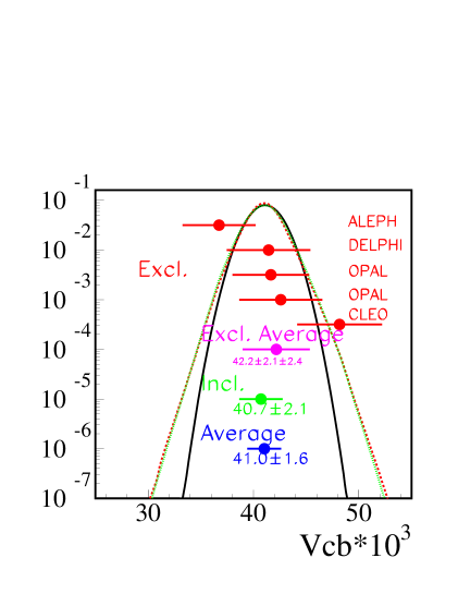
The inclusive measurements of the semileptonic branching fraction of $b$-hadrons give instead

$$\left|{V}_{cb}\right|=(40.7\pm 0.5\pm 2.0)\times 10^{-3}\,.$$ (42)

The interested reader may consult [70] for more details on the quoted uncertainty for inclusive decays.

The combination of all results, using the procedure explained previously when averaging $F(1)\,\left|{V}_{cb}\right|$ measurements, taking into account correlated systematics, gives

$$\left|{V}_{cb}\right|=(41.0\pm 1.6)\times 10^{-3}\,.$$ (43)

The corresponding p.d.f, which has been used in the present analysis, is shown in Figure 1.

5.2 Extraction of $\left|{V}_{ub}\right|$

Figure 2: The p.d.f. for $\left|{V}_{ub}\right|$.

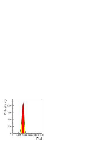
$\left|{V}_{ub}\right|$ has been obtained from the measurements done at CLEO and LEP. The CLEO collaboration [71] has measured the branching fraction for the decay $\bar{{B^{0}_{d}}}\rightarrow\rho^{+}\ell^{-}\bar{\nu_{\ell}}$ and deduced a value for $\left|{V}_{ub}\right|$ using several models to describe the decay form factors. LEP collaborations [72] have developed dedicated algorithms to be sensitive to a large fraction of the inclusive decay rate $b\rightarrow u\ell^{-}\bar{\nu_{\ell}}$ and, with some assumptions, a value for $\left|{V}_{ub}\right|$ is obtained. The two measurements are

$$\left|{V}_{ub}\right| = (32.5\pm 2.9\pm 5.5)\times 10^{-4}\quad\mbox{CLEO}$$

$$\left|{V}_{ub}\right| = (41.3\pm 6.3\pm 3.1)\times 10^{-4}\quad\mbox{LEP}\,$$ (44)

where the second uncertainty is theoretical. The p.d.f. for the CLEO measurement is thus a convolution of a Gaussian and a flat distribution. The theoretical error for the LEP measurement, being the convolution of several different errors, is taken from a Gaussian distribution [72]. Combining the two distributions, in practice we obtain almost a Gaussian p.d.f. (see Figure 2) corresponding to

$$\left|{V}_{ub}\right|=(35.5\pm 3.6)\times 10^{-4}.$$ (45)

5.3 The parameter $\lambda$

Figure 3: Probability distribution function for $\lambda$ obtained by combining measurements of $\left|{V}_{ud}\right|$ and $\left|{V}_{us}\right|$. The full line distribution corresponds to a Gaussian whereas the dotted curve is obtained using the procedure explained in the text.

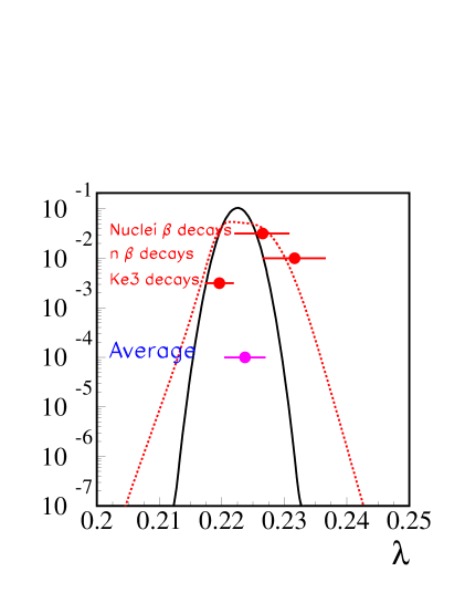
Measurements of $\left|{V}_{ud}\right|$ and $\left|{V}_{us}\right|$ reported in [31] have been combined using the procedure explained in Section 5.1, assuming that $\left|{V}_{ud}\right|=\cos{\theta_{c}}$ and $\left|{V}_{us}\right|=\sin{\theta_{c}}\equiv\lambda$. The additional contribution from $\left|{V}_{ub}\right|^{2}$ to the unitarity condition can be safely neglected owing to present uncertainties. The p.d.f. for $\lambda$ strongly deviates from a Gaussian (see Figure 3) because present determinations of this quantity from $\left|{V}_{ud}\right|$ and $\left|{V}_{us}\right|$ measurements are more than two standard deviations away. The average and the standard deviation of the obtained distribution correspond to

$$\lambda=0.2237\pm 0.0033$$ (46)

whereas a classical fit gives $\lambda=0.2225\pm 0.0019$.
Using the values of $\left|{V}_{cb}\right|$ and $\lambda$ given respectively in Equations (43) and (46) the following result is obtained for the parameter A

$$A=\frac{\left|{V}_{cb}\right|}{\lambda^{2}}=0.819\pm 0.040$$ (47)

It may be noticed that, in the present determination of the $\bar{\rho}$ and $\bar{\eta}$ parameters, $\left|{V}_{cb}\right|$ and $\lambda$, but not A, are used as constraints.

6 A new procedure to include the information coming from ${B}^{0}_{s}-\bar{{B}}^{0}_{s}$ oscillation analyses

In this Section, we illustrate a new procedure to include in the analysis the experimental searches for ${B}^{0}_{s}-\bar{{B}}^{0}_{s}$ mixing. It makes use of the likelihood along the lines discussed in Section 3.

The study of $B^{0}_{s}-\bar{B}^{0}_{s}$ oscillations is done by introducing the oscillation amplitude ${\cal A}$ as explained in [73]. Events have been distributed in two classes corresponding to oscillating and non-oscillating candidates, according to the information obtained by tagging the presence of a $B$ or a $\bar{B}$ meson at the beam interaction time and at the $b$-hadron decay time. The expected decay-time distribution of events is obtained by using a function which contains time distributions for all components, taking into account the non-perfect event classification, the different behaviour of $b$-hadron decays, which depend on their type ($\bar{B}^{0}_{d}$, ${B^{-}}$, $\bar{B}^{0}_{s}$ or $b$-baryon), and background components originating from charm and light flavours. The time distribution for the oscillating (non-oscillating) signal is given by

$${\cal P}(B^{0}_{s}\rightarrow\bar{B}^{0}_{s}(B^{0}_{s}))=\frac{1}{2\tau_{B^{0}_{s}}}(1-(+){\cal A}\cos{\Delta m_{s}t})e^{-t/\tau_{B^{0}_{s}}}\,.$$ (48)

Such theoretical time distributions have been convoluted with the expected time resolution of the measurements. For each value of $\Delta m_{s}$ and each analysis, the oscillation amplitude ${\cal A}$ is fitted. Fitted amplitude values have been combined [32] using a common set of determinations for external parameters and taking into account possible correlations between the different analyses. In this respect the use of the oscillation amplitude provides a simple framework to account for all these effects. The 95$\%$ C.L. limit on $\Delta m_{s}$ corresponds to the value $\Delta m_{s}^{lim}$ for which ${\cal A}+1.645~{}\sigma_{\cal A}$ = 1, whereas the sensitivity $\Delta m_{s}^{sens}$ corresponds to $1.645~{}\sigma_{\cal A}$ = 1. It is the value of $\Delta m_{s}$ at which it is expected that the 95$\%$ limit will be set, if ${\cal A}$ = 0. In addition, the final likelihood distribution can be retrieved from the combined amplitudes corresponding to all analyses as explained in the following.

The information coming from oscillation amplitude measurements, which gives constraints on possible values of $\Delta m_{s}$, was included [13, 14, 15, 23, 24], up to now, using the distribution 

$${\rm F}(\Delta m_{s})=~{}\exp{-\frac{1}{2}\left(\frac{{\cal A}-1}{\sigma_{\cal A}}\right)^{2}}.$$ (49)

Recently it has been proposed to use the log-likelihood function $\Delta\log{\cal L}^{\infty}(\Delta m_{s})$ referenced to its value obtained for $\Delta m_{s}=\infty$ [74]. Similar considerations, developed in a different context, have been detailed in [45]. The log-likelihood values can be easily deduced from $\cal A$ and $\sigma_{\cal A}$ using the expressions given in [73]

$$\Delta\log{\cal L}^{\infty}(\Delta m_{s}) =\frac{\textstyle 1}{\textstyle 2}\,\left[\left(\frac{\textstyle{\cal A}-1}{\textstyle\sigma_{\cal A}}\right)^{2}-\left(\frac{\textstyle{\cal A}}{\textstyle\sigma_{\cal A}}\right)^{2}\right] =\left(\frac{\textstyle 1}{\textstyle 2}-{\cal A}\right){\textstyle 1\over\textstyle\sigma_{\cal A}^{2}}\ ,$$ (50)

$$\Delta\log{\cal L}^{\infty}({\Delta m_{s}})_{mix} =-\frac{1}{2}\frac{1}{\sigma_{\cal A}^{2}}\ ,$$ (51)

$$\Delta\log{\cal L}^{\infty}({\Delta m_{s}})_{nomix} =\frac{1}{2}\frac{1}{\sigma_{\cal A}^{2}}\ .$$ (52)

The last two equations give the average log-likelihood value when $\Delta m_{s}$ corresponds to the true oscillation frequency (mixing case) and when $\Delta m_{s}$ is far from the oscillation frequency ($|\Delta m_{s}-\Delta m_{s}^{true}|\gg\Gamma/2$, no-mixing case). $\Gamma$ is the full width at half maximum of the amplitude distribution in case of a signal; typically $\Gamma\simeq{1}/{\tau_{B^{0}_{s}}}$. In the following it is shown that:

• Equation (49) does not represent the optimal way to include the $\Delta m_{s}$ information.
  In particular it is incorrect in case of a measurement;

• Equation (50) allows to define the likelihood ratio R

  $${\rm R}(\Delta m_{s})=e^{\textstyle{-\Delta\log{\cal L}^{\infty}(\Delta m_{s})}}=\frac{{\cal L}(\Delta m_{s})}{{\cal L}(\Delta m_{s}=\infty)}\ .$$ (53)

  The function R corresponds to the ratio of probability densities for different $\Delta m_{s}$ values. The absolute $\Delta m_{s}$ probability density, instead, remains undefined because ${\cal L}(\Delta m_{s})$ stays constant for $\Delta m_{s}$ values much larger than the sensitivity; in this region R is equal to unity.

• a reasonable procedure to extrapolate $\rm R$ in regions where the direct measurements of the amplitudes are not available can be established.

6.1 Comparison between the new and the old methods

The main concern, in the previous approach, was that the sign of the deviation with respect to the value ${\cal A}=1$ was not used, whereas it is expected that an evidence for a signal would manifest itself by giving an amplitude value which is simultaneously compatible with ${\cal A}=1$ and incompatible with ${\cal A}=0$.

The new method, at variance, includes the relative weight of the two hypotheses. Equations (50) and (53) show that $\rm R$ has a clear interpretation as ratio between two cases: mixing (${\cal A}=1$) or no mixing (${\cal A}=0$). The properties of the log-likelihood ratio, R, and its application in Higgs boson searches have been introduced in [75].
Another problem of the previous approach is that the sign of the deviation of the amplitude with respect to unity is not considered: this implies that a lower probability is attributed to $\Delta m_{s}$ values with ${\cal A}>1$ with respect to $\Delta m_{s}$ values having ${\cal A}=1$. Since this behaviour is clearly undesired, in the old method the amplitudes larger than unity have been set to unity (as it has been implicitly done in [13]-[15]).
The difference between the old and the new method are illustrated in two cases:

• a single analysis having the sensitivity at 15 ps^-1 (see next paragraph and Figure 4) simulating a signal at $\Delta m_{s}=5$ps^-1 (this value has been chosen well below the sensitivity in order to amplify the effect).

• the world average analysis (see Figure 5)

Figure 4: Amplitude analysis with $\Delta m_{s}$ generated at 5 $\mbox{ps}^{-1}$: a) amplitude spectrum, b) $\Delta\log{\cal L}^{\infty}(\Delta m_{s})$, c) comparison between R and the function F used in the previous method. The maxima of the two functions have been rescaled to unity in order to ease the comparison

Figure 5: World average amplitude analysis: a) amplitude spectrum, b) $\Delta\log{\cal L}^{\infty}(\Delta m_{s})$, c) comparison between ${\rm R}$ and the function used in the previous method.

In Figure 4-a and Figure 4-b, respectively, the amplitude spectrum ${\cal A}$ and the corresponding distribution for $\Delta{\cal L}^{\infty}(\Delta m_{s})$ are given for the simulated case, in which there is a signal at $\Delta m_{s}=5~{}{\rm ps}^{-1}$. Figure 4-c shows that there is a marked difference between the behaviour of ${\rm R}$ and ${\rm F}$. While the function $\rm R$ shows, by construction, a maximum corresponding to the fitted value ($\Delta m_{s}=(5.10\pm 0.25)~{}\mbox{ps}^{-1}$), the function $\rm F$ is not able to spot the maximum, in particular it attributes large probability to any $\Delta m_{s}$ value with ${\cal A}\sim 1$ regardless its error.
For the world average analysis, Figure 5 shows that the agreement between $\rm R$ and $\rm F$ is acceptable only when ${\cal A}\sim 0$.

6.2 How to treat $\Delta m_{s}$ regions without amplitude measurements?

The procedure used to continue $\rm R$ beyond the last measured amplitude value ($\Delta m_{s}^{last}$) is based on the continuation of the amplitude spectrum from which $\rm R$ is deduced:

• continuation of $\sigma(\cal A)$: the behaviour of $\sigma(\cal A)$ for $\Delta m_{s}>\Delta m_{s}^{lim}$ can be reproduced by tuning the parameters of a fast simulation (toy-MC). The method used here is similar to the one presented in  [76]. The errors on the amplitude can be written as:

  $$\sigma^{-1}({\cal A})=\sqrt{N}\,\eta_{{B_{s}}}\,(2\epsilon-1)\,W(\sigma_{L},\sigma_{P},\Delta m_{s})$$

  where $N$ is the total number of events, $\eta_{{B_{s}}}$ the purity of the sample in ${B_{s}}$ decays, $\epsilon$ the purity of the tagging at the decay time, $\sigma_{L}$ is the ${B_{s}}$ flight length uncertainty and $\sigma_{P}$ the relative uncertainty on its momentum. The parameters $\sigma_{L}$, $\sigma_{P}$ and the global factor that multiply $W$ have been obtained by adjusting the simulated error distribution on the one measured with real events.

  Figure 6 shows the agreement between the toy-MC calculation and real data for $\Delta m_{s}<\Delta m_{s}^{last}$ (the upper bound on $\Delta m_{s}$ of the amplitude plot for which there are measurements) and the extrapolation to higher values. It has been verified (with an independent toy-MC) that the extrapolated errors approximate well the simulated error distribution.

• continuation of $\cal A$: this part is more critical than the previous one. In particular it is more sensitive to the real amplitude spectrum. Nevertheless if $\Delta m_{s}^{sens}<<\Delta m_{s}^{last}$, the significance $S$ ($S={\cal A}/\sigma_{\cal A}$) is approximately constant.

In the following the amplitudes at $\Delta m_{s}>25~{}\mbox{ps}^{-1}$ (which corresponds to $\Delta m_{s}^{last}$ for the combined world average plot) are deduced using the extrapolation of the amplitude errors and fixing the significance at the last measured value. As a consequence, for $\Delta m_{s}$ values larger than $\Delta m_{s}^{last}$, R is fixed to the last measured point. Although this procedure is reasonable, it should be stressed that it is very desirable to have all the amplitudes (with errors) up to the $\Delta m_{s}$ value where $\rm R$ approaches its plateau.

Figure 6: Comparison between the error distribution computed with a toy-MC (solid line) and the measured amplitude errors (circles).

6.3 The likelihood function $\rm R$ used in the analysis

The present world average on $\Delta m_{s}$ shows an “hint” of signal at $\Delta m_{s}\sim$ 17.5 ps^-1 (see Figure 5-b). Its significance (about 2.2 $\sigma$) is not sufficient to claim evidence for an observation of the ${B}^{0}_{s}-\bar{{B}}^{0}_{s}$ oscillation. This effect is in fact larger than the average value, of $\sim 1.2\,\sigma$, which is expected in case of a real signal in that region.
Whatever conclusion can be drawn from these data, it should be stressed that:

• the likelihood function $\rm R$ deduced from data contains the present knowledge on $\Delta m_{s}$ and it is the optimal weight function to be used in the fit;

• the use of $\rm R$ does not imply any assumption either on the evidence or on the presence of a signal. It only translates the experimental fact that the log-likelihood function has a minimum at 17.5 ps^-1 with a $2.2~{}\sigma$ significance.

Figure 7: Comparison between different weight functions used in the fit. The curve determined by the continuous and dashed lines corresponds to the likelihood ratio obtained with, respectively, the measured amplitudes and the extrapolation to large values of $\Delta m_{s}$. The dotted curve is obtained by truncating the previous distribution once the amplitude becomes larger than one.

Although we believe that the use of $\rm R$ is, indeed, the best method to include the information on $\Delta m_{s}$, we briefly mention some alternative approaches. The main difference is that, with these methods, a fraction of the available experimental information is lost.

1. 95% C.L. limit: this method uses a stepwise function starting at $\Delta m_{s}^{lim}$. We mention it only for completeness since the choice of the C.L. is arbitrary.

2. Min($\rm R$,1): in this approach it is considered that no value of $\Delta m_{s}$ has to be preferred with respect to $\Delta m_{s}=\infty$ (only exclusion is possible). It was used in our preliminary analyses [58] and consists in setting ${\cal A}=0.5$ for all amplitudes having larger values (see equation (50). Since there is no reason to throw away the information contained in amplitudes with values ranging between 0.5 and 1, this method has been abandoned.

3. Min[${\rm R}(A=1)$,$\rm R$]: in this method one tries to avoid biases induced by “lucky” fluctuations. The strategy is then to limit the likelihood ratio to the value obtained when the amplitude reaches ${\cal A}=1$ for the first time. The effect is to flatten the ratio R around its maximum.

Two different definitions of $\rm R$ have then been used as weight function in the fitting procedure:

• the complete $\rm R$ distribution deduced from data and from the toy-MC;

• the function Min[${\rm R}(A=1)$,$\rm R$].

They are shown in Figure 7 and the second choice has been considered as a “pessimistic” approach to evaluate the induced variation on the fitted quantities in Section 8.

7 Results and discussion

In this Section we give the results for the quantities of interest. Values of the hadronic parameters, which can be determined quite accurately by assuming the validity of the Standard Model, are also extracted. The central value is always given using the average, and the error corresponds to the standard deviation. For asymmetric p.d.f. we also give the median and the error corresponds to regions containing 34% probability on each side of the median.

7.1 Results obtained with all measurements

Figure 8: Allowed regions for $\bar{\rho}$ and $\bar{\eta}$ using the parameters listed in Table 1. The contours at 68%, 95%, 99% and 99.9% probability are shown. The full lines correspond to the central values of the constraints given by the measurements of $\left|V_{ub}\right|/\left|V_{cb}\right|$, $\left|\varepsilon_{K}\right|$ and $\Delta m_{d}$. The two dotted curves correspond, from left to right respectively, to the 95% upper limit and to the value of the sensitivity obtained from the experimental study of ${B}^{0}_{s}-\bar{{B}}^{0}_{s}$ oscillations.

Figure 9: The allowed regions for $\bar{\rho}$ and $\bar{\eta}$ (contours at 68%, 95%) are compared with the uncertainty bands (at 68% and 95% probabilities) for $\left|V_{ub}\right|/\left|V_{cb}\right|$, $\left|\varepsilon_{K}\right|$, $\Delta m_{d}$ and the limit on $\Delta m_{s}/\Delta m_{d}$ (dotted curve).

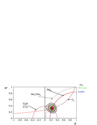
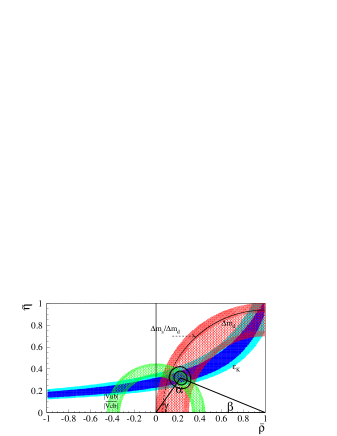
The region in the ($\bar{\rho},~{}\bar{\eta})$ plane selected by the measurements of $\left|\varepsilon_{K}\right|$, $\left|V_{ub}/V_{cb}\right|$, $\Delta m_{d}$ and from the information on $\Delta m_{s}$ (using the R function of Figure 7) is given in Figure 8. In Figure 9 the uncertainty bands for the quantities, obtained using Equations (1)–(4), are presented. Each band, corresponding to only one of the constraints, contains 68% and 95% of the events obtained by varying the input parameters. This comparison illustrates the consistency of the different constraints provided by the Standard Model. In the present studies, two statistically equivalent procedures have been used. They differ in the way values for $\bar{\rho}$ and $\bar{\eta}$ have been extracted and in the inclusion of QCD corrections to $\epsilon_{K}$ and to ${B}^{0}-\bar{{B}}^{0}$ mixing, which are either computed [19] or taken as independent inputs [14]. The measured values of the two parameters are

$$\bar{\rho}=0.224\pm 0.038,~{}\bar{\eta}=0.317\pm 0.040$$ (54)

and

$$\bar{\rho}=0.221\pm 0.037,~{}\bar{\eta}=0.315\pm 0.039\ ,$$ (55)

using the methods of ref. [14] and [19] respectively. The two quantities are practically uncorrelated (correlation coefficient of -5%), as it can be seen from the contour plot of Figure 8. Fitted values for the angles of the unitarity triangle have been obtained also

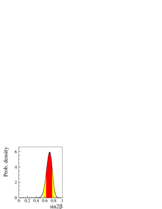
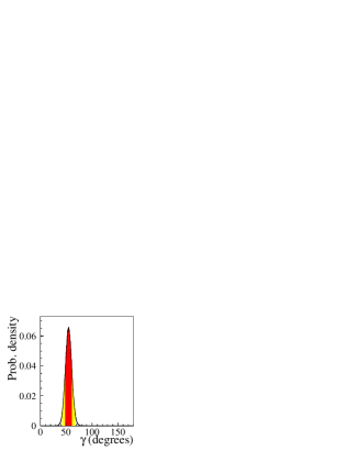
$$\sin(2\,\beta)=0.698\pm 0.066\,,\quad\sin(2\,\alpha)=-0.42\pm 0.23\,,\quad\gamma=(54.8\pm 6.2)^{\circ}\quad\cite[cite]{[\@@bibref{}{ref:parodietal}{}{}]}$$ (56)

(the quoted error is symmetric, in spite of the small asymmetry of the distributions shown in Figure 10) and

$$\sin(2\beta)=0.692\pm 0.065\,,\quad\sin(2\alpha)=-0.43\pm 0.21\,,\quad\gamma=(54.9\pm 5.7)^{\circ}\quad\cite[cite]{[\@@bibref{}{ref:roma}{}{}]}.$$ (57)

respectively.

The results in the two approaches are in agreement and, in the following, quoted values and figures are those obtained using the approach of [14]. In Figure 10, the p.d.f. for the angles of the unitarity triangle are given.

Figure 10: The p.d.f. for $\sin(2\alpha)$, $\sin(2\beta)$ and $\gamma$ . The red (darker) and the yellow (clearer) zones correspond respectively to 68% and 95% of the normalised area.

Few comments can be made:

• $\sin(2\beta)$ is determined quite accurately. This value has to be compared with recent measurements of this quantity using $J/\psi K_{S}$ events from LEP [77], CDF [78], BaBar [79] and BELLE [80]. The accuracies of these measurements are completely dominated by the statistical errors and their average is $\sin(2\beta)=0.49\pm 0.16$.

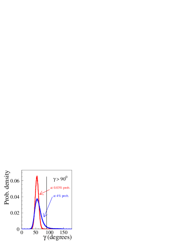
• the angle $\gamma$ is known within an accuracy of about 10%. It has to be stressed that, with present measurements, the probability that $\gamma$ is greater than 90^∘ is only 0.03%. Without including the information from $\Delta m_{s}$, it is found that $\gamma$ has 4% probability to be larger than 90^∘. The central value for the angle $\gamma$ is much smaller than that obtained in recent fits of rare $B$-meson two-body decays [81]. It remains to be seen to which extent the results of [81] are affected by the model dependence in the theoretical description of two-body decays. In this respect, it would be interesting to examine under which conditions these decays can be described by the same value of $\gamma$ as found in the present study. An exploratory work in this direction can be found in [82].

7.2 The CKM triangle from $b$-physics alone

As four constraints are used to determine the values of two parameters, it is possible to relax, in turn, one (or more) of these constraints, still obtaining significant confidence intervals. An interesting exercise consists in removing the theoretical constraint for $\hat{B}_{K}$ in the measurement of $\left|\varepsilon_{K}\right|$ ([18]-[83]). The corresponding selected region in the ($\bar{\rho},~{}\bar{\eta})$ plane is shown in Figure 11, where the region selected by the measurement of $\left|\varepsilon_{K}\right|$ alone is also drawn. This comparison shows that the Standard Model picture of CP violation in the $K$ system and of $B$ decays and oscillations are consistent. In the same figure, we also compare the allowed regions in the ($\bar{\rho},~{}\bar{\eta})$ plane with those selected by the measurement of $\sin(2\,\beta)$ using $J/\psi K_{S}$ events.

Figure 11: The allowed regions (at 68%, 95%, 99% and 99.9% probability) for $\bar{\rho}$ and $\bar{\eta}$ using the constraints given by the measurements of $\left|V_{ub}\right|/\left|V_{cb}\right|$, $\Delta m_{d}$ and $\Delta m_{s}$. The constraint due to $\left|\varepsilon_{K}\right|$ is not included. The regions (at 68% and 95% probability) selected by the measurements of $\left|\varepsilon_{K}\right|$ (continuous (1$\sigma$) and dotted (2$\sigma$) curves) and $\sin(2\,\beta)$ (darker (1$\sigma$) and clearer (2$\sigma$) zones) are shown. For $\sin(2\,\beta)$ the two solutions are displayed.

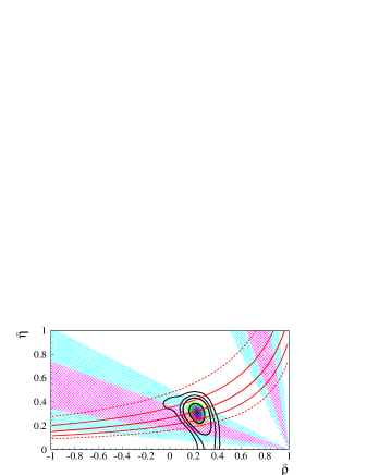
Using constraints from $b$-physics alone the following results are obtained

$$\bar{\eta}=0.302^{+0.052}_{-0.061}\quad; \quad[0.145-0.400]\quad\rm{at}~{}95\%\quad; >0.08~{}\rm{at}~{}99\%$$

$$\sin(2\,\beta)=0.678^{+0.078}_{-0.101}\quad; [0.392-0.818]\quad\rm{at}~{}95\%$$ (58)

(in terms of average and standard deviation the results are $\bar{\eta}$ = 0.296 $\pm$ 0.063 and $\sin(2\,\beta)$ = 0.663 $\pm$ 0.109).
Another way for illustrating the agreement between $K$ and $B$ measurements consists in comparing the values of the $\hat{B}_{K}$ parameter obtained in lattice QCD calculations with the value extracted from Equation (4), using the values of $\bar{\rho}$ and $\bar{\eta}$ selected by $b$-physics alone

$$\hat{B}_{K}^{\rm b-phys}=0.90^{+0.30}_{-0.14}, 0.64\leq\hat{B}_{K}^{\rm b-phys}\leq 1.8~{}{\rm at}~{}95\%~{}{\rm probability}$$ (59)

(in terms of average and standard deviation the result is $\hat{B}_{K}^{\rm b-phys}$ = 0.97 $\pm$ 0.23).
Since $\hat{B}_{K}$ is not limited from above, for the present study, probabilities are normalised assuming $\hat{B}_{K}<$5. The p.d.f of $\hat{B}_{K}^{\rm b-phys}$ is shown in Figure 12.

Figure 12: The p.d.f. for $\hat{B}_{K}^{\rm b-phys}$ .

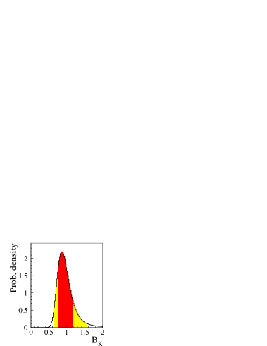
It can be noticed that the values of two theoretical parameters, namely $f_{B_{d}}\sqrt{\hat{B}_{B_{d}}}$ and $\xi$ have been used to obtain this result. Hopefully, when accurate direct measurements of $\sin(2\,\beta)$ will become available, it will be possible to remove another theoretical input (or even all of them).

7.3 The expected value for $\Delta m_{s}$

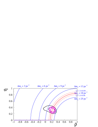
Figure 13 shows the allowed region for $\bar{\rho}$ and $\bar{\eta}$ obtained when removing the constraint coming from the study of $B^{0}_{s}$–$\bar{B}^{0}_{s}$ mixing. It illustrates the importance of the use of this information. This can be illustrated also, from the p.d.f. of the angle $\gamma$ obtained with or without including the $\Delta m_{s}$ constraint (see Figure 14). High values for $\gamma$ are excluded at high confidence level by the experimental lower limit on $\Delta m_{s}$.

Figure 13: The allowed regions for $\bar{\rho}$ and $\bar{\eta}$ using the constraints given by the measurements of $\left|\varepsilon_{K}\right|$, $\left|V_{ub}\right|/\left|V_{cb}\right|$ and $\Delta m_{d}$ at 68% and 95% probability are shown by the thin contour lines. Selected regions for $\bar{\rho}$ and $\bar{\eta}$ when the constraint due to $\Delta m_{s}$ is included have been superimposed using thick lines. The different continuous circles correspond to fixed values of $\Delta m_{s}$. Dashed circles, drawn on each side of the curve corresponding to $\Delta m_{s}=18.0~{}ps^{-1}$, indicate the effect of a variation by $\pm 0.06$ on $\xi$.

Figure 14: The p.d.f. for $\gamma$ obtained with (red-clearer) and without (blue-darker) including the $\Delta m_{s}$ constraint. The vertical line corresponds to $\gamma$ = 90^∘. The probabilities of $\gamma>$ 90^∘ are also given.

Figure 15: Probability distribution of $\Delta m_{s}$. The information from ${B}^{0}_{s}-\bar{{B}}^{0}_{s}$ oscillations is used(not used) (distribution on the right(left).

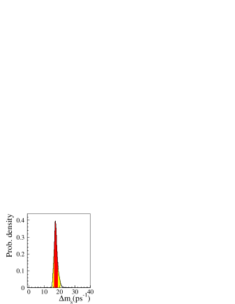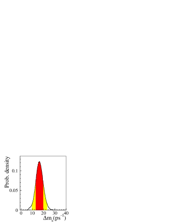
It is also possible to extract the probability distribution for $\Delta m_{s}$, which is shown in Figures 15 (see also [84]). From this distribution one obtains

$$\Delta m_{s}=(16.3\pm 3.4)\ {\rm ps}^{-1}\,\quad\quad 9.7\leq\Delta m_{s}\leq 23.2~{}{\rm ps}^{-1}\quad{\rm at}~{}95\%\ {\rm probability}.$$ (60)

If the information from the ${B}^{0}_{s}-\bar{{B}}^{0}_{s}$ analyses is included, results become

$$\Delta m_{s}=(17.3^{+1.5}_{-0.7})\ {\rm ps}^{-1}\,\quad\quad 15.6\leq\Delta m_{s}\leq 20.5~{}{\rm ps}^{-1}\quad{\rm at}~{}95\%\ {\rm probability}$$ (61)

(in terms of average and standard deviation the result is $\Delta m_{s}$ = (17.7 $\pm$ 1.3)${\rm ps}^{-1}$).
These values are in agreement with the recent estimate of $\Delta m_{s}=15.8(2.3)(3.3)\ ps^{-1}$, presented in [51].

7.4 Determination of $f_{B_{d}}\sqrt{\hat{B}_{B_{d}}}$

The value of $f_{B_{d}}\sqrt{\hat{B}_{B_{d}}}$ can be obtained by removing the theoretical constraint coming from this parameter in ${B}^{0}_{d}$–$\bar{B}^{0}_{d}$ oscillations.

Figure 16: The p.d.f. for $f_{B_{d}}\sqrt{\hat{B}_{B_{d}}}$.

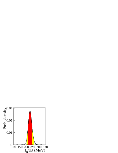
Using the two other theoretical inputs, $\hat{B}_{K}$ and $\xi$ , $f_{B_{d}}\sqrt{\hat{B}_{B_{d}}}$ is measured with an accuracy which is better than the current evaluation from lattice QCD, given in Section 4. From the p.d.f. shown in Figure 16,

$$f_{B_{d}}\sqrt{\hat{B}_{B_{d}}}=(231\pm 15)\,\rm MeV\,$$ (62)

is obtained. The present analysis shows that these results are in practice very weakly dependent on the exact value taken for the uncertainty on $f_{B_{d}}\sqrt{\hat{B}_{B_{d}}}$. An evaluation of this effect has been already presented in [15] where the flat part of the theoretical uncertainties on $f_{B_{d}}\sqrt{\hat{B}_{B_{d}}}$ was multiplied by two. Similar tests will be shown in Section 8.

7.5 Further comments on the Lattice predictions for $f_{B_{d}}\sqrt{\hat{B}_{B_{d}}}$ and $\hat{B}_{K}$

The values found in the present analysis for $f_{B_{d}}\sqrt{\hat{B}_{B_{d}}}$ and $\hat{B}_{K}$ are in agreement with those of previous studies [14]–[20]. They are also in agreement with the predictions from lattice QCD. It can be noticed that lattice predictions for these quantities existed well before it were possible to extract them from the analysis of the unitarity triangle. Moreover these predictions have been stable over the years: one of the first calculations of $B_{K}$ gave $B_{K}^{\overline{\rm MS}}(\mu=2\,{\rm GeV})=0.65\pm 0.15$ [85] in 1987 (corresponding to $\hat{B}_{K}=0.90\pm 0.20$) and $\hat{B}_{K}$ was estimated to be $\hat{B}_{K}=0.84\pm 0.03\pm 0.14$ in 1996 [44]; a compilation by one of the authors of the present paper gave $f_{B_{d}}\sqrt{\hat{B}_{B_{d}}}=(220\pm 40)$ MeV and $f_{B_{d}}\sqrt{\hat{B}_{B_{d}}}=(207\pm 30)$ MeV, in 1995 and 1996 respectively [86].

7.6 Lower bounds on $f_{B_{d}}\sqrt{\hat{B}_{B_{d}}}$ and $\hat{B}_{K}$

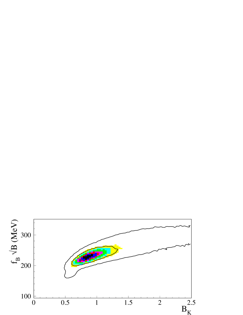
The region in the plane ($f_{B_{d}}\sqrt{\hat{B}_{B_{d}}}$, $\hat{B}_{K}$), which is obtained by removing the theoretical constraints on these quantities, is shown in Figure 17. It appears that present constraints can cope with very large values of $\hat{B}_{K}$ and thus it was needed to restrict the possible range of variation for this parameter. In the present study, probabilities have been normalised assuming $\hat{B}_{K}<\rm{5}$. The 68% and 95% probability contours have rather different shapes. Within 68% probability, both $f_{B_{d}}\sqrt{\hat{B}_{B_{d}}}$ and $\hat{B}_{K}$ are well constrained. The most important conclusion which can be drawn from this study is the simultaneous lower bounds on $f_{B_{d}}\sqrt{\hat{B}_{B_{d}}}$ and $\hat{B}_{K}$, namely

$$\hat{B}_{K}>0.5\,\quad{\rm and}\quad\quad f_{B_{d}}\sqrt{\hat{B}_{B_{d}}}>150\,\,\mbox{MeV}\,,\quad{\rm at~{}95}\%~{}\mbox{probability}.$$ (63)

Figure 17: The 68% and 95% contours in the $(f_{B_{d}}\sqrt{\hat{B}_{B_{d}}}$,$\hat{B}_{K})$ plane.

7.7 Other quantities of interest

For completeness the values of the phases $\chi$, $\chi^{\prime}$ and $\mbox{Im}\,\lambda_{t}$ [87] are also given.

$$\chi = {\rm arg}\left(-\frac{V_{cs}^{*}V_{cb}}{V_{ts}^{*}V_{tb}}\right)\quad={\rm atan}\left(\frac{\bar{\eta}}{1+\lambda^{2}\bar{\rho}}\right)\,,$$

$$\chi^{\prime} = {\rm arg}\left(-\frac{V_{ud}^{*}V_{us}}{V_{cd}^{*}V_{cs}}\right)\quad={\rm atan}\left(\frac{(\left|{V}_{cb}\right|^{2}\bar{\eta})}{1-\lambda^{2}/2-(\left|{V}_{cb}\right|^{2}/2)(1-2\bar{\rho})}\right)\,,$$

$$\quad\mbox{Im}\,\lambda_{t}\quad = \lambda\left|{V}_{cb}\right|^{2}\bar{\eta}\,.$$ (64)

The measured values of these parameters are

$$\chi=(17.4\pm 2.1)^{\circ},\quad ~{}\chi^{\prime}=(0.031\pm 0.003)^{\circ},\quad \mbox{Im}\,\lambda_{t}=(1.19\pm 0.12)~{}10^{-4}\,.$$ (65)

8 Stability of the results

The sensitivity of present results on the assumed probability distributions attached to the input parameters was studied. The comparison of the results obtained by varying the size of the theoretical uncertainties has been done to evaluate the sensitivity to these variations of uncertainties quoted on fitted values. This must not be taken as a proposal to inflate the uncertainties obtained in the present analysis.

Parameter(s)	Modified Value(s)	$\bar{\rho}$	$\bar{\eta}$
All	None	$0.224\pm 0.038$	$0.317\pm 0.040$
${\hat{B}_{K}}$	$0.87\pm 0.06\pm 0.26$	$0.225\pm 0.040$	$0.314\pm 0.045$
$f_{B_{d}}\sqrt{\hat{B}_{B_{d}}}$	$(230\pm 25\pm 40)\rm MeV$	$0.224\pm 0.039$	$0.318\pm 0.041$
$\xi$	1.14 $\pm$ 0.04 $\pm$ 0.10	$0.221\pm 0.045$	$0.318\pm 0.042$
$\left|{V}_{ub}\right|$	(37.8 $\pm$ 4.9) 10-4	$0.240\pm 0.044$	$0.334\pm 0.048$
$\left|{V}_{cb}\right|$	(40.7 $\pm$ 2.6) 10-3	$0.224\pm 0.039$	$0.320\pm 0.048$
$\Delta m_{s}$ cons.	see Sect. 6	$0.227\pm 0.047$	$0.315\pm 0.042$
All	as above	$0.249\pm 0.064$	$0.333\pm 0.065$

Table 4: Stability tests (1). Central values and uncertainties for $\bar{\rho}$ and $\bar{\eta}$ have been defined relative to the median of the corresponding p.d.f.

Parameter(s)	Modified value(s)	$\sin{(2\beta)}$	$\sin{(2\alpha)}$	$\gamma$(degrees)
All	None	$0.698\pm 0.066$	$-0.42\pm 0.23$	$54.8\pm 6.2$
${\hat{B}_{K}}$	$0.87\pm 0.06\pm 0.26$	$0.693\pm 0.071$	$-0.45\pm 0.26$	$54.5\pm 6.7$
$f_{B_{d}}\sqrt{\hat{B}_{B_{d}}}$	$(230\pm 25\pm 40)\rm MeV$	$0.698\pm 0.067$	$-0.44\pm 0.24$	$54.9\pm 6.3$
$\xi$	1.14 $\pm$ 0.04 $\pm$ 0.10	$0.697\pm 0.067$	$-0.42\pm 0.26$	$55.4\pm 7.2$
$\left|{V}_{ub}\right|$	(37.8 $\pm$ 4.9) 10-4	$0.733\pm 0.080$	$-0.40\pm 0.24$	$54.4\pm 6.1$
$\left|{V}_{cb}\right|$	(40.7 $\pm$ 2.6) 10-3	$0.701\pm 0.077$	$-0.43\pm 0.26$	$54.8\pm 6.6$
$\Delta m_{s}$ cons.	see Sect. 6	$0.698\pm 0.067$	$-0.45\pm 0.27$	$54.6\pm 7.6$
All	as above	$0.738^{+0.086}_{-0.101}$	$-0.42\pm 0.37$	$53.3\pm 10.0$

Table 5: Stability tests (2). Central values and uncertainties for $\sin{(2\beta)}$, $\sin{(2\alpha)}$ and $\gamma$ have been defined relative to the median of the corresponding p.d.f.

In these tests, all values for uncertainties of theoretical origin have been, in turn, multiplied by two. For the quantities $\left|{V}_{ub}\right|$ and $\left|{V}_{cb}\right|$, new p.d.f. have been determined, following the prescriptions given in Sections 5.1 and 5.2 and used in the analysis; central values and uncertainties quoted in Tables 4 and 5 correspond to the average and standard deviation of these distributions.

The main conclusion of this exercise is that, even in the case where all theoretical uncertainties are doubled, the unitarity triangle parameters are determined with an uncertainty which increases only by about 1.5 (see Tables 4 and 5).

9 Comparison between the standard and the 95% C.L. scanning approaches

parameter	Value $\pm$ Gaussian $\pm$ Flat errors
$\left|V_{cb}\right|$	$(40.0\pm 2.0\pm 0.0)\times 10^{-3}$
$\left|V_{ub}\right|$	$(34.0\pm 1.4\pm 5.0)\times 10^{-4}$
$\Delta m_{d}$	$(0.473\pm 0.016\pm 0.000)$  ps-1
$\Delta m_{s}$	$>$ 14.3 ps-1
$\left|\varepsilon_{K}\right|$	$(2.285\pm 0.018\pm 0.000)\times 10^{-3}$
$B_{K}$	$0.80\pm 0.00\pm 0.15$
$f_{B_{d}}\sqrt{\hat{B}_{B_{d}}}$	$(200\pm 0\pm 40)~{}\rm MeV$
$\xi=\frac{f_{B_{s}}\sqrt{\hat{B}_{B_{s}}}}{f_{B_{d}}\sqrt{\hat{B}_{B_{d}}}}$	$1.14\pm 0.00\pm 0.08$

Table 6: Values of the quantities used in the comparison between the standard and the 95% C.L. scanning methods. The quoted flat error values are used to define the range of variation of the corresponding parameter in the 95% C.L. scanning approach and to define the uniform probability distribution for this parameter in the standard method.

The theoretical basis which allows to define, in the standard approach, regions of the $(\bar{\rho},\bar{\eta})$ plane which correspond to any given value of confidence has been already discussed. For completeness, in this Section, a comparison of present results at the 95% C.L. with the corresponding regions selected using the 95% C.L. scanning approach is made. In the latter approach, this region is the envelope of 95% C.L. contours defined at several points and, as discussed previously, it is not easy to understand to which level of confidence they correspond to.

The results of the study given in [24] have been used in this comparison and the same central values for the parameters have been used in the two cases. When, in the 95% C.L. scanning approach, a parameter is scanned over a given interval, in the standard approach a flat probability distribution defined over the same range has been used. In Table 6 central values and uncertainties used in this comparison, taken from [24], have been collected.

parameter	standard approach	95% C.L. scanning approach
	(95%  prob. range)
$\bar{\rho}$	$-0.06,~{}0.31$	$0.00,~{}0.30$
$\bar{\eta}$	$0.26,~{}0.42$	$0.20,~{}0.45$
$\sin(2\,\beta)$	$0.56,~{}0.82$	$0.50,~{}0.85$

Table 7: Comparison of standard and 95% C.L. scanning approaches. Note that intervals quoted for the results of the standard approach correspond to 95% probability for each quantity, whereas in the 95% C.L. scanning method the intervals are obtained from the maximum and minimum values spanned by the 2-D envelope.

Figure 18: The contour corresponding to 95% probability in the standard approach, given by the external continuous line, has been compared with the region spanned by 95% C.L. ellipses obtained in the 95% C.L. scanning method. The internal contour, corresponding to 68% probability in the standard approach, is also drawn.

Figure 19: Left: Probability distribution of the $\bar{\rho}$ variable obtained in the standard approach. The interval selected in the ‘95% C.L. scanning method has been indicated. Right: Comparison between different input distributions for the parameter $f_{B_{d}}\sqrt{\hat{B}_{B_{d}}}$ and the final probability distribution obtained with all constraints but the measurement of $\Delta m_{d}$.

The constraint coming from the study of ${B}^{0}_{s}-\bar{{B}}^{0}_{s}$ oscillations is included using the weight given in Equation (49), since it was used also in the 95% C.L. scanning analysis.

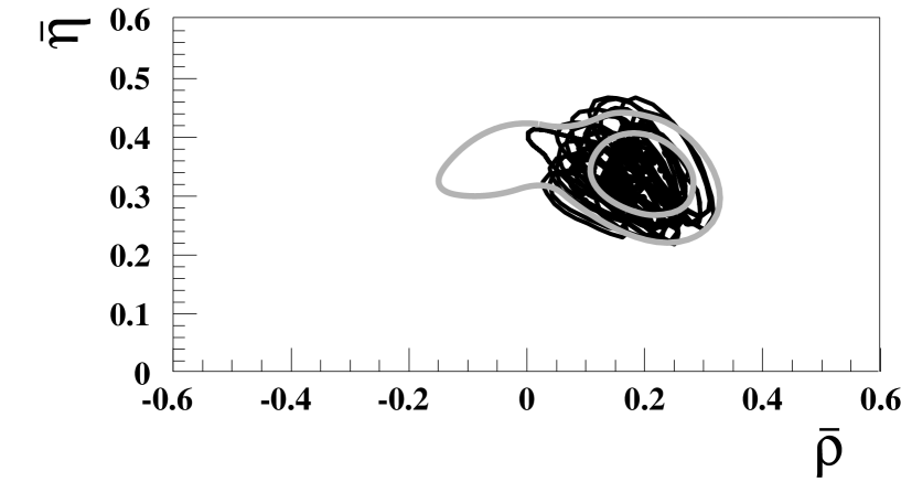
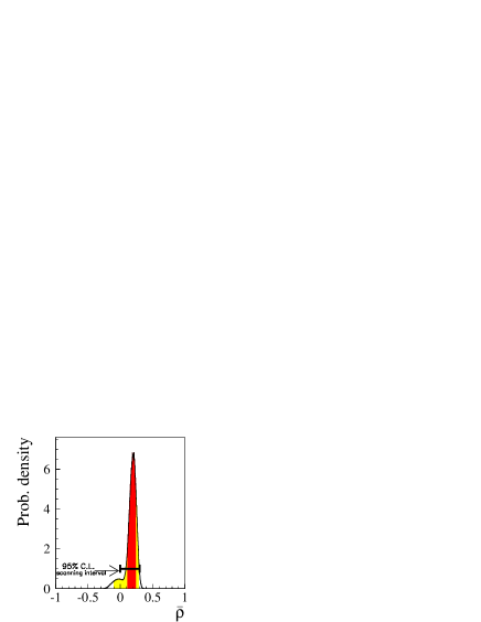
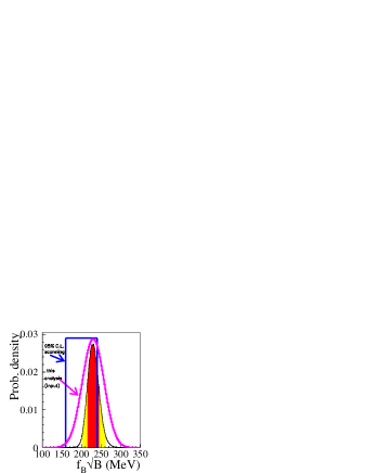
In Figure 18 the “95% C.L.” contours obtained with the two methods have been compared and the 95% C.L. intervals for $\bar{\rho}$ and $\bar{\eta}$ are given in Table 7. In Figure 19-left the distribution of $\bar{\rho}$ is also shown.

Several remarks are in order:

• when using the same values for the input parameters and for their uncertainties, the 95% C.L. scanning and the standard approaches select similar regions in the $(\bar{\rho},~{}\bar{\eta})$ plane. It is then unjustified to qualify as too optimistic the standard approach. The main difference is precisely the opposite, namely that, unlike the case of 95% C.L. scanning, with the standard method one is able to quantify the confidence corresponding to any given interval.

• in the standard approach the probability distribution in the $(\bar{\rho},~{}\bar{\eta}$) plane is meaningful. In the present exercise, the interval $[0.15,~{}0.30]$ for $\bar{\rho}$ is more probable than $[0.,~{}0.15]$. Quoting simply that the value of $\bar{\rho}$ is expected to be between 0 and 0.3, at 95% C.L. does not indicate that there is a most probable value around 0.2. Such considerations are not in order in the 95% C.L. scanning approach;

• even in the 95% C.L. scanning approach it is necessary to define intervals which are expected to contain the true values of the parameters. But then some probability has to be attributed to these intervals. It is thus illusory the statement that with this method one does not attribute any probability distribution to the theoretical inputs. Indeed the statement that an input cannot assume a value outside a given interval, is equivalent to attribute zero probability to the region outside the interval;

• the flat distribution for a theoretical parameter, in some cases, is a very strong a-priori, as illustrated in Figure 19-right, where the choice of the central value and error on $f_{B}\sqrt{\hat{B}_{B}}$ used in [24] is shown. The flat interval corresponds to the values quoted in Table 6. The broad Gaussian-like distribution, used in the present analysis, results from a convolution between a flat and a Gaussian distributions using the parameters of Table 1. This is also shown in the figure, together with the final p.d.f. resulting from our analysis. From this comparison, it appears that the region favoured by present measurements is marginally compatible with the interval selected in the 95% C.L. scanning. In particular, the latter excludes a priori (large) values of $f_{B}\sqrt{\hat{B}_{B}}$ which are still compatible with data.

10 Conclusions

In this paper, we have discussed the inferential framework which allows a consistent analysis of the unitarity triangle, where both experimental and theoretical uncertainties play an important role. In particular, we were concerned with the treatment of the theoretical errors, which raised several controversies in the past. We have shown that, in this framework, there is a consistent way of handling the theoretical uncertainties and that these can be included in the analysis in a way similar to the experimental ones. The main results of our analysis have been discussed in Section 7 and, for convenience, are listed below (see Table 8).

Present measurements of $\left|\varepsilon_{K}\right|$, $\left|V_{ub}/V_{cb}\right|$, $\Delta m_{d}$ and of the limit on $\Delta m_{s}$ allow, within the framework of the Standard Model, and after including results from lattice QCD on $\hat{B}_{K}$, $f_{B_{d}}\sqrt{\hat{B}_{B_{d}}}$ and $\xi$, to determine the parameters of the CKM unitarity triangle.

Parameters	Present analysis
$\bar{\rho}$	0.224 $\pm$ 0.038
$\bar{\eta}$	0.317 $\pm$ 0.040
$\sin(2\,\beta)$	0.698 $\pm$ 0.066
$\sin(2\alpha)$	-0.42 $\pm$ 0.23
$\gamma$	(54.8 $\pm$ 6.2)∘

Table 8: The results on the unitarity triangle parameters presented in this paper.

The dependence of central values and quoted uncertainties on values and uncertainties assumed for the theoretical parameters, and on different procedures to include the available information, have been evaluated. These exercises demonstrate that the standard approach employed to get our numbers is on a sound basis and that results and uncertainties for the quantities of interest are stable. The determination of central values and uncertainty distributions for the theoretical inputs used in the present analysis has been reviewed and explained.

By removing, in turn, the different constraints it has been verified that, within the present uncertainties, the Standard Model description of CP violation is in agreement with the measurements. In particular, $B$ oscillations and decays select, in the $(\bar{\rho},~{}\bar{\eta})$ plane, a similar region as $\left|\varepsilon_{K}\right|$ for the $K^{0}$ system. This constitutes already a test of compatibility between the measurements of the sides and of the angles of the CKM triangle. Its accuracy is given by the quoted uncertainties on $\hat{B}_{K}$ appearing in the first row of Table 9.
This Table gives a summary of the determination of the values of some theoretical parameters and of $\Delta m_{s}$ obtained in the present analysis and corresponding estimates from lattice QCD:

Parameters	Present analysis	Present analysis	Lattice QCD
	(with the contraint)	(without the contraint)
$\hat{B}_{K}$	$0.88\pm 0.08$	$0.90^{+0.30}_{-0.14}$	$0.87\pm 0.06\pm 0.13$
$f_{B_{d}}\sqrt{\hat{B}_{B_{d}}}$	$(230\pm 12)$ MeV	$(231\pm 15)$ MeV	$(230\pm 25\pm 20)$ MeV
$\Delta m_{s}$	$(17.3^{+1.5}_{-0.7})$ ps-1	$(16.3\pm 3.4)$ ps-1	$(15.8\pm 2.3\pm 3.3)$ ps-1

Table 9: Comparison between the values of the parameters determined in the present analysis with those obtained by lattice QCD. In the second row (third row) the results are obtained including (not including) the given constraint.

Values of the parameters given in Table 9 and of the angles reported in Table 8 can be considered as reference numbers to which new measurements, using different approaches, can be compared in view of identifying new physics contributions.

Three results will become available in a near future.

• Analyses of $B$-meson two body decays have already produced values for $\gamma$ which were more than 2$\sigma$ larger than the value given in Table 8. Including recent results form BaBar and Belle Collaborations, smaller values of the angle $\gamma$ are preferred [79],[80]. Before claiming evidence of new physics, a better theoretical understanding of non-leptonic decays and more stable measurements are needed.

• Direct measurements of sin2$\beta$ obtained studying $J/\psi K_{S}$ events at $B$ factories or at TeVatron will provide important tests when the accuracy of these measurements will be better than 0.1.

• Finally, a first evidence of ${B}^{0}_{s}-\bar{{B}}^{0}_{s}$ oscillations could still come from LEP and SLD Collaborations and accurate measurements are expected from the TeVatron. Measured values larger than 25 $\rm{ps^{-1}}$ could provide evidence for new physics.

References

-
[1]
N. Cabibbo, Phys. Rev. Lett. 10 (1963) 531;
M. Kobayashi and T. Maskawa, Prog. Theor. Phys. 49 (1973) 652. - [2] L. Wolfenstein, Phys. Rev. Lett. 51 (1983) 1945.
- [3] A.J. Buras, M.E. Lautenbacher and G. Ostermaier, Phys. Rev. D50 (1994) 3433.
- [4] G. Buchalla, A.J. Buras and M.E. Lautenbacher, Rev. Mod. Phys. 68 (1996) 1125.
- [5] M. Lusignoli, L. Maiani, G. Martinelli and L. Reina, Nucl. Phys. B369 (1992) 139.
[6]
A. Ali and D. London, in Proceeding of “ECFA Workshop on the Physics of a
Meson Factory”, Ed. R. Aleksan, A. Ali (1993);
A. Ali and D. London, hep-ph/9405283;
A. Ali and D. London, in Proceeding of “27th International Conference on High Energy Physics (ICHEP95)”, Glasgow, Scotland, 20-27 July 1994, hep-ph/9409399;
A. Ali and D. London, Z. Phys. C65 (1995) 431. - [7] S. Herrlich and U. Nierste, Phys. Rev. D52 (1995) 6505.
- [8] M. Ciuchini, E. Franco, G. Martinelli, L. Reina and L. Silvestrini, Z. Phys. C68 (1995) 239.
[9]
A. Ali and D. London, Nuovo. Cim. 109A (1996) 957;
A. Ali, Acta Physica Polonica B 27 (1996) 3529;
A. Ali and D. London, Nucl. Phys. 54A (1997) 297. -
[10]
A.J. Buras, Invited talk at “7th International Symposium on Heavy Flavour Physics”,
Santa Barbara, CA, 7-11 July 1997, hep-ph/9711217;
A. J. Buras and R. Fleischer, in Heavy Flavours II, World Scientific (1997), eds. A.J. Buras and M. Linder, hep-ph/9704376. - [11] R. Barbieri, L.J. Hall, S. Raby and A. Romanino, Nucl. Phys. B493 (1997) 3.
- [12] A. Ali and B. Kayser, invited article in ’The Particle Century”, Inst. of Physics Publ., Inc., Bristol and Philadelphia, 1998, Ed. Gordon Fraser, hep-ph/9806230.
- [13] P. Paganini, F. Parodi, P. Roudeau and A. Stocchi, Phys. Scripta V. 58 (1998) 556.
- [14] F. Parodi, P. Roudeau and A. Stocchi, Nuovo Cim. 112A (1999) 833.
- [15] F. Caravaglios, F. Parodi, P. Roudeau, A. Stocchi, hep-ph/0002171, talk at “BCP 99”, Taipei, Taiwan Dec. 3-7 1999, to appear in the Proceedings.
- [16] S. Mele, Phys. Rev. D59 (1999) 113011.
- [17] A. Ali and D. London, Eur. Phys J. C9 (1999) 687.
- [18] P. Checchia, E. Piotto, F. Simonetto, Eur. Phys. Lett. 47 (1999) 113011.
- [19] M. Ciuchini, E. Franco, L. Giusti, V. Lubicz and G. Martinelli, Nucl. Phys. B573 (2000) 201.
- [20] M. Bargiotti et al., La Rivista del Nuovo Cimento Vol. 23N3 (2000) 1.
- [21] see e.g. A.J. Buras, M. Jamin and M.E. Lautenbacher, Phys. Lett. B389 (1996) 749.
- [22] G. D’Agostini, hep-ex/9910036.
- [23] BaBar Physics book, Chapter 14, p. 933.
- [24] S. Plaszczynski, M.-H. Schune, hep-ph/9911280.
- [25] A. Falk, talk given at the “19th International Symposium on Lepton and Photon Interactions at High-Energies (LP 99)”, Stanford, CA, 9-14 Aug 1999, hep-ph/9908520.
- [26] S. Stone, talk given at “Heavy Flavours 8”, Southampton, UK, 1999, to appear in the Proceedings, hep-ph/9910417.
- [27] T. Inami and C.S. Lim, Prog. Theor. Phys. 65 (1981) 297; ibid. 65 (1981) 1772.
- [28] A.J. Buras, M. Jasmin and P.H. Weisz, Nucl. Phys. B347 (1990) 491.
[29]
F. Abe et al., CDF Collaboration, Phys. Rev. Lett.
74 (1995) 2626;
S. Abachi et al., D0 Collaboration, Phys. Rev. Lett. 74 (1995) 2632. -
[30]
S. Herrlich and U. Nierste, Nucl. Phys. B419 (1994) 192;
G. Buchalla, A.J.Buras and M.E. Lautenbacher, Rev. Mod. Phys. 68, (1996) 1125. - [31] Review of Particle Physics, Eur. Phys. J. C15 (2000) 1.
- [32] The LEP B Oscillation Working Group, http://lepbosc.web.cern.ch/LEPBOSC/, LEPBOSC 98/3.
- [33] V. Gimenez, L. Giusti, G. Martinelli and F. Rapuano, JHEP 0003 (2000) 018.
- [34] G. D’Agostini, CERN Report 99–03.
- [35] G. D’Agostini and M. Raso, hep-ex/0002056.
- [36] M. Bochicchio et al., Nucl. Phys. B262 (1985) 331.
- [37] M. Lüscher, Les Houches Lectures on “Advanced Lattice QCD”, hep-lat/9802029, and refs. therein.
- [38] C. Bernard, T. Blum and A. Soni, Nucl. Phys. (Proc. Suppl.) 53 (1997) 382; Phys. Rev. D58 (1998) 014501.
- [39] V. Lubicz, review talk given at the “XX Physics in Collision”, Lisboa, Portugal, June 29th–July 1st 2000, to appear in the Proceedings, hep-ph/0010071.
- [40] S. Aoki, review talk given at “19th International Symposium on Lepton and Photon Interactions at High-Energies (LP 99)”, Stanford, California, 9-14 Aug 1999, hep-ph/9912288.
- [41] S. Hashimoto, review talk given at the “17th International Symposium on Lattice Field Theory (LATTICE 99)”, Pisa, Italy, 29 Jun - 3 Jul 1999, hep-lat/9909136.
- [42] C. Bernard, review talk given at the 18th International Symposium on Lattice Field Theory (LATTICE 2000), Bangalore, India, 17 - 22 August 2000, to appear in the Proceedings.
- [43] S.R. Sharpe, talk given at “29th International Conference on High-Energy Physics (ICHEP 98)”, Vancouver, Canada, 23-29 Jul 1998, hep-lat/9811006.
- [44] S.R. Sharpe, Nucl. Phys. (Proc.Suppl.) 53 (1997) 181.
- [45] G. D’Agostini, hep-ex/0002055.
- [46] C.R. Allton et al., Phys. Lett. B405 (1997) 133.
- [47] A.X. El-Khadra et al., Phys. Rev. D58 (1998) 014506.
- [48] S. Aoki et al., Phys. Rev. Lett. 80 (1998) 5711.
- [49] C. Bernard et al., Phys. Rev. Lett. 81 (1998) 4812.
- [50] D. Becirevic et al., Phys. Rev. D60 (1999) 074501.
- [51] D. Becirevic et al., BUHEP-00-3, hep-lat/0002025.
- [52] K.C. Bowler et al., EDINBURGH-2000-14, hep-lat/0007020.
- [53] C. Bernard et al., talk given by S. Datta at the “18th International Symposium on Lattice Field Theory (Lattice 2000)”, Bangalore, India, 17-22 Aug 2000, hep-lat/0011029.
- [54] A. Ali Khan et al., UTCCP-P-68, hep-lat/0010009.
- [55] L. Lellouch and C. J. Lin, (UKQCD Collaboration), hep-ph/0011086.
- [56] S. Aoki et al., Nucl. Phys. (Proc.Suppl.) 47 (1996) 433.
- [57] V. Gimenez and J. Reyes, Nucl. Phys. B545 (1999) 576.
[58]
A. Stocchi, hep-ph/0010222, talk at “XXXth ICHEP 27” Jul.-2 Aug. 2000, Osaka, Japan, to appear in the
Proceedings;
F. Parodi , talk at “International Conference on CP Violation Physics”, 8-22 Sep. 2000, Ferrara, Italy, to appear in the Proceedings;
A. Stocchi, hep-ph/0012215 talk at “International Conference on -Physics at Hadron Machines - Beauty2000” Kibbutz Maagan, Israel, Sep. 13-18,2000, to appear in the Proceedings. - [59] S. Collins et al., Phys. Rev. D60 (1999) 074504.
- [60] G. Kilcup, R. Gupta and S. R. Sharpe, Phys. Rev. D57 (1998) 1654.
- [61] G.P. Lepage and P.B. Mackenzie, Phys. ReV. D48(1993) 2250.
- [62] G. Kilcup, D. Pekurovsky and L. Ventakataraman, Nucl. Phys. (Proc. Suppl.) 53 (1997) 345.
- [63] R. Gupta, Lecture at the “XVI Autumn school and Workshop on fermion masses, mixing and CP violation”, Lisboa, Portugal, 6-15 October 1997, hep-ph/9801412; Nucl. Phys. (Proc. Suppl.) 63 (1998) 278.
- [64] L. Lellouch, review talk given at the 18th International Symposium on Lattice Field Theory (LATTICE 2000), Bangalore, India, 17 - 22 August 2000, to appear in the Proceedings, hep-lat/0011088.
- [65] LEP Working group on , http://lepvcb.web.cern.ch/LEPVCB/.
- [66] J.P. Alexander et al., CLEO Collaboration, CLEO CONF 00-03.
- [67] M.J. Schervish, Am. Stat. 50 (1996) 203.
- [68] G. Cowan, “Statistical data analysis”, Oxford, 1998.
- [69] G. D’Agostini, CERN-EP/99-139 and hep-ex/9910036.
- [70] “Combined results on -hadron production rates, lifetimes, oscillations and semileptonic decays”, ALEPH, CDF, DELPHI, L3, OPAL and SLD Collaborations, SLAC-PUB-8492 and CERN-EP-2000-096.
- [71] B.H. Behrens et al., CLEO Collaboration, Phys. Rev. D61 (2000) 052001.
- [72] LEP Working group on , http://battagl.home.cern.ch/battagl/vub/vub.html.
- [73] H.G. Moser and A. Roussarie, Nucl. Instr. and Methods A 384 (1997) 491.
- [74] P. Checchia, E. Piotto, F. Simonetto, hep-ph/9907300.
- [75] G. D’Agostini and G. Degrassi, Eur. Phys. J. C10 (1999) 633.
- [76] G. Boix and D. Abbaneo, Journal of High Energy Physics 9908 (1999) 004.
- [77] R. Barate et al. (ALEPH Collaboration) Phys. Lett. B492 (2000), 259-274. K. Ackerstaff et al. (OPAL Collaboration) Eur. Phys. C5 (1998) 379.
- [78] T. Affolder at al. Phys. ReV. D61 (2000) 072005.
- [79] B. Aubert et al. (Babar Collaboration) hep-ex/0102030
- [80] A. Abashian et al. (Belle Collaboration) hep-ex/0102018
[81]
M. Gronau and J.L. Rosner, Phys. Rev. D61 (2000) 073008;
X.-G. He, W.-S. Hou and K.-C. Yang, Phys. Rev. Lett. 83 (1999) 1100;
W.-S. Hou and K.-C. Yang, hep-ph/9908202;
W.-S. Hou, J.G. Smith and F. Würthwein,hep-ex/9910014;
H.-Y. Cheng and K.-C. yang, hep-ph/9910291;
B. Dutta and S. Oh, hep-ph/9911263. - [82] Y.F. Zhou, Y.L. Wu, J.N. Ng and C.Q. Geng, hep-ph/0006225.
- [83] R. Barbieri, L. Hall, A. Stocchi and N. Weiner, Phys. Lett. B425 (1998) 119;
- [84] D. Jaffe, S. Youssef, Comput.Phys.Commun. 101 (1997) 206
- [85] M.B. Gavela et al., Nucl. Phys. B306 (1988) 677.
- [86] G. Martinelli, Nuovo Cimento Vol. 109 N.6-7 (1996) 787 and Nucl. Instr. and Methods in Phys. Research A384 (1996) 241.
- [87] BTeV Collaboration, hep-ex/0006037.