Statistical Analysis of Solar Neutrino Data

Abstract

We calculate with Monte Carlo the goodness of fit and the confidence level of the standard allowed regions for the neutrino oscillation parameters obtained from the fit of the total rates measured in solar neutrino experiments. We show that they are significantly overestimated in the standard method. We also calculate exact allowed regions with correct frequentist coverage. We show that the exact VO, LMA and LOW regions are much larger than the standard ones and merge together giving an allowed band at large mixing angles for all $\Delta{m}^{2}\gtrsim 10^{-10}\,\mathrm{eV}^{2}$.

1 Introduction

The data of solar neutrino experiments provide strong indications in favor of neutrino oscillations and their statistical analysis give indications on the values of the neutrino mixing parameters. For two neutrino generations, these parameters are the mass-squared difference $\Delta{m}^{2}\equiv m_{2}^{2}-m_{1}^{2}$, where $m_{1}$ and $m_{2}$ are the two neutrino masses, and $\tan^{2}\theta$, where $\theta$ is the mixing angle (see, for example, Ref.[1]).

In this paper we present statistical methods based on Monte Carlo numerical calculations that allow to improve the standard statistical analysis of solar neutrino data, which is approximate [2]. We consider the data relative to the total rates measured in the Homestake and Super-Kamiokande experiments, and the weighted average of the total rates measured in the two Gallium experiments GALLEX and SAGE, as given in Table I of Ref.[3].

As in the standard method, we use as estimator of $\Delta{m}^{2}$ and $\tan^{2}\theta$ the global minimum $X^{2}_{\mathrm{min}}$ of the least-squares function

$$X^{2} = \sum_{j_{1},j_{2}=1}^{N_{\mathrm{exp}}}\left(R^{\mathrm{(thr)}}_{j_{1}}-R^{\mathrm{(exp)}}_{j_{1}}\right)(V^{-1})_{j_{1}j_{2}}$$ (1)

$$\hskip 28.45274pt\times\left(R^{\mathrm{(thr)}}_{j_{2}}-R^{\mathrm{(exp)}}_{j_{2}}\right)\,,$$

where $N_{\mathrm{exp}}=3$ is the number of experimental data points, $V$ is the covariance matrix of experimental and theoretical uncertainties, $R^{\mathrm{(exp)}}_{j}$ is the event rate measured in the $j^{\mathrm{th}}$ experiment and $R^{\mathrm{(thr)}}_{j}$ is the corresponding theoretical event rate, that depends on $\Delta{m}^{2}$ and $\tan^{2}\theta$. We calculate the covariance matrix $V$ following the standard method (see, for example, Ref.[3]), with the correction proposed in Ref.[4].

The standard procedure to calculate the allowed regions in the neutrino oscillation parameter space (see, for example, Ref.[3]) is based on the assumption that $X^{2}$ has a $\chi^{2}$ distribution with $N_{\mathrm{exp}}$ degrees of freedom. This would be correct if the theoretical rates $R^{\mathrm{(thr)}}_{j}$ depended linearly on the parameters to be determined in the fit and the errors of $R^{\mathrm{(thr)}}_{j}-R^{\mathrm{(exp)}}_{j}$ were multinormally distributed with constant covariance matrix $V$. In this case there should be only one minimum of $X^{2}$ and the allowed regions at $100\beta\%$ confidence level (CL), given by $X^{2}\leq X^{2}_{\mathrm{min}}+\Delta{X^{2}}(\beta)$, should be elliptical.

It is well-known that in reality there are several local minima of $X^{2}$, each one determining an allowed region, and these allowed regions do not have elliptic form (see, for example, Ref.[3]). This is due to the fact that the requirements above are not satisfied. In particular, the stronger effect is due to the non-linear dependence of the theoretical rates $R^{\mathrm{(thr)}}_{j}$ from the parameters, which generates several local minima of $X^{2}$.

In the following two sections we present estimations of the goodness of fit (Section 2) and the confidence level of the standard allowed regions (Section 3) obtained with a Monte Carlo calculation of the distribution of $X^{2}$. In Section 4 we present the results of a Monte Carlo calculation of allowed regions with exact coverage.

Figure 1: Allowed 90%, 95%, 99%, 99.73% CL regions. The gray areas are the allowed regions with exact frequentist coverage. The areas enclosed by the solid lines are the standard allowed regions.

2 Goodness of Fit

Goodness of fit (GOF) is the probability to find a value of the global minimum $X^{2}_{\mathrm{min}}$ of $X^{2}$ larger than the one obtained from the fit. Since there are more than one local minima of $X^{2}$ with relatively close values of $X^{2}$, there are more possibilities to obtain good fits of the data with respect to the case of one minimum, and the true goodness of fit is smaller than the one obtained with the standard method.

We calculate the distribution of $X^{2}_{\mathrm{min}}$ assuming that the best-fit values $\widehat{\Delta{m}^{2}}$, $\widehat{\tan^{2}\theta}$ of $\Delta{m}^{2}$, $\tan^{2}\theta$ are reasonable surrogates of the true unknown values $\Delta{m}^{2}_{\mathrm{true}}$, $\tan^{2}\theta_{\mathrm{true}}$ and the probability distribution of the differences $\widehat{\Delta{m}^{2}}_{(k)}-\widehat{\Delta{m}^{2}}$, $\widehat{\tan^{2}\theta}_{(k)}-\widehat{\tan^{2}\theta}$ is not too different from the true distribution of the differences $\widehat{\Delta{m}^{2}}_{(k)}-\Delta{m}^{2}_{\mathrm{true}}$, $\widehat{\tan^{2}\theta}_{(k)}-\tan^{2}\theta_{\mathrm{true}}$ in a large set of best-fit parameters $\widehat{\Delta{m}^{2}}_{(k)}$, $\widehat{\tan^{2}\theta}_{(k)}$ ($k=1,2,\ldots$) obtained with hypothetical experiments.

Using $\widehat{\Delta{m}^{2}}$, $\widehat{\tan^{2}\theta}$ as surrogates of the true values, we generate $N_{s}$ synthetic random data sets with the usual gaussian distribution for the experimental and theoretical uncertainties. We apply the least-squares method to each synthetic data set, leading to an ensemble of simulated best-fit parameters $\widehat{\Delta{m}^{2}}_{(s)}$, $\widehat{\tan^{2}\theta}_{(s)}$ with $s=1,\ldots,N_{s}$, each one with his associated $(X^{2}_{\mathrm{min}})_{s}$. Then we calculate the goodness of the fit as the fraction of simulated $(X^{2}_{\mathrm{min}})_{s}$ in the ensemble that are larger than the one actually observed, $X^{2}_{\mathrm{min}}$.

The global minimum of the least-squares function (1), $X^{2}_{\mathrm{min}}=0.42$, occurs in the SMA region for $\Delta{m}^{2}=5.1\times 10^{-6}\,\mathrm{eV}^{2}$ and $\tan^{2}\theta=1.6\times 10^{-3}$. The Monte Carlo method yields a GOF of 40%, that must be compared with the 52% GOF obtained with the standard method. Therefore, the standard method significantly overestimates the GOF.

3 Confidence Level of Allowed Regions

The allowed regions with $100\beta\%$ CL are defined by the property that they belong to a set of allowed regions, obtained with hypothetical experiments, which cover (i.e. include) the true value of the parameters with probability $\beta$. This property is called coverage.

When there are several local minima of $X^{2}$ with relatively close values of $X^{2}$, in repeated experiments the global minimum has significant chances to occur far from the true (unknown) value of the parameters, leading to a smaller probability that the allowed regions cover the true value with respect to the case in which there is only one minimum, which is assumed for the validity of the standard method for the calculation of allowed regions. Hence, the true confidence level of a standard $100\beta\%$ CL allowed region is smaller than $\beta$.

We estimate the true confidence level of the standard $100\beta\%$ CL allowed regions using the best fit values of the parameters, $\widehat{\Delta{m}^{2}}$, $\widehat{\tan^{2}\theta}$, as surrogates of the true values, $\Delta{m}^{2}_{\mathrm{true}}$, $\tan^{2}\theta_{\mathrm{true}}$, for the generation of a large number of synthetic data sets. We apply the standard procedure to each synthetic data set and obtain the corresponding standard $100\beta\%$ CL allowed regions in the space of the neutrino oscillation parameters. Then we count the number of synthetic standard $100\beta\%$ CL allowed regions that cover the assumed surrogate $\widehat{\Delta{m}^{2}}$, $\widehat{\tan^{2}\theta}$ of the true values. The ratio of this number and the total number of synthetically generated data set gives a Monte Carlo estimation $\beta_{\mathrm{MC}}$ of the true confidence level of the standard $100\beta\%$ CL allowed regions.

We obtained that the confidence level of the standard 90% CL allowed regions is 86%, which is significantly smaller. Other results are presented in Ref.[2].

4 Exact Allowed Regions

The calculation of the confidence level of the standard allowed regions presented in the previous section is approximate, because it is based on the assumption of a surrogate for the unknown true values of the neutrino oscillation parameters. It would be useful to be able to calculate exact allowed with the desired confidence level, i.e. with correct coverage. The procedure that allows to perform this task has been invented by Neyman in 1937 (see references in Ref.[2]). Let us emphasize that this procedure gives allowed regions with proper coverage for any unknown true values of the parameters.

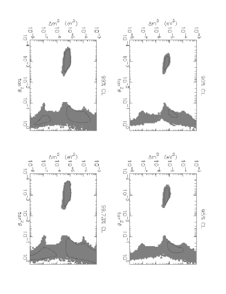
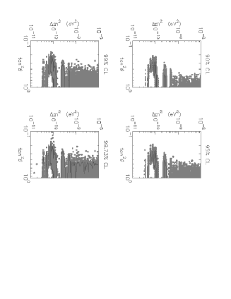
Our implementation of Neyman’s procedure for the calculation of the allowed regions in the $\tan^{2}\theta$–$\Delta{m}^{2}$ plane is described in details in Ref.[2]. The results are presented in Fig.1, where the gray areas are the exact allowed regions, and the standard allowed regions are enclosed by solid lines. One can see that the exact LMA, LOW and VO regions are much larger than the standard ones and there is no separation between them. Hence, large mixing angles with $0.2\lesssim\tan^{2}\theta\lesssim 1$ are allowed for $\Delta m^{2}\gtrsim 10^{-10}\,\mathrm{eV}^{2}$. On the other hand, the exact SMA region approximately coincides with the standard one. This is due to the fact that in the SMA region the assumption of a linear dependence of the theoretical rates $R^{\mathrm{(thr)}}_{j}$ in Eq.(1) from the parameters $\tan^{2}\theta$, $\Delta m^{2}$ is approximately correct, whereas it is violated quite badly in the LMA, LOW and VO regions.

5 Conclusions

In conclusion, we have shown that the standard method used in the analysis of solar neutrino data in terms of neutrino oscillations significantly overestimates the goodness of fit and the confidence level of the allowed regions. We have also calculated allowed regions with correct coverage. The SMA region approximately coincides with the standard one, but the VO, LMA and LOW regions are much larger than the standard ones and merge together giving an allowed band at large mixing angles for all $\Delta{m}^{2}\gtrsim 10^{-10}\,\mathrm{eV}^{2}$.

References

- [1] S. M. Bilenky, C. Giunti, and W. Grimus, Prog. Part. Nucl. Phys. 43, 1 (1999).
- [2] M. V. Garzelli and C. Giunti, hep-ph/0007155.
- [3] M. C. Gonzalez-Garcia et al., Nucl. Phys. B573, 3 (2000), hep-ph/9906469.
- [4] M. V. Garzelli and C. Giunti, Phys. Lett. B488, 339 (2000), hep-ph/0006026.