Investigation of meson loop effects in the Nambu–Jona-Lasinio model
Vom Fachbereich Physik
der Technischen Universität Darmstadt
zur Erlangung des Grades
eines Doktors der Naturwissenschaften
(Dr. rer. nat.)
genehmigte Dissertation von
Dipl.-Phys. Micaela Oertel
aus Langen (Hessen)
Darmstadt 2000
D17

Abstract

The influence of mesonic fluctuations on quantities in the Nambu–Jona-Lasinio model is examined. To that end different approximation schemes are introduced which guarantee the consistency with several relations following from chiral symmetry. In particular this refers to the Goldstone theorem, which states the existence of massless bosons, in our case pions, if the symmetry of the Lagrangian is spontaneously broken. The Gell-Mann–Oakes–Renner relation describes the behavior of the pion mass for small current quark masses, which explicitly break chiral symmetry. Three different schemes are presented. These are the inclusion of the ring sum in a so-called “$\Phi$-derivable-method”, an expansion in powers of $1/N_{c}$ and an expansion up to one-meson loop in the effective action formalism. Since the two latter schemes are used for explicit calculations, it is explicitely proved that the Goldstone theorem as well as the Gell-Mann–Oakes–Renner relation hold within those schemes.

The influence of meson-loop effects on the quark condensate $\langle{\bar{\psi}\psi}\rangle$, the pion mass, the pion decay constant $f_{\pi}$ and properties of $\rho$- and $\sigma$-meson are investigated. First we focus on the determination of a consistent set of parameters. In the $1/N_{c}$-expansion scheme it is possible to find a set of parameters which allows to simultaneously describe the quantities in the pion sector and those related to the $\rho$-meson, whereas this turns out to be not possible within the expansion of the effective action. Results for the $\sigma$-meson are also discussed. Here, similarly to the $\rho$-meson, mesonic intermediate states are essential. Besides, the relation of our model to hadronic models is discussed.

In the last part of this thesis the behavior of the quark condensate at nonzero temperature is studied. In the low-temperature region agreement with the model independent chiral perturbation theory result in lowest order can be obtained. The perturbative $1/N_{c}$-expansion scheme does not allow for an examination of the chiral phase transition at higher temperatures, whereas this is possible within the meson-loop approximation scheme. A first order phase transition is found.

feyngph

Introduction

Since the substructure of the nucleus was discovered at the beginning of the century one tries to understand in which way its constituents, the nucleons, interact. Already in the thirties Yukawa suggested [1] that this interaction could be described by an exchange of a massive meson which was later identified with the pion. Presently this idea is still the basis for most phenomenological models of the interaction between nucleons which mainly rely on the exchange of mesons with various quantum numbers [2, 3].

Not only our present notion of the interaction between nucleons, but almost all phenomenological models which try to describe strongly interacting particles, mesons and baryons, in the low-energy region, are essentially influenced by the idea of Yukawa. These models incorporate mesons and baryons as the principal degrees of freedom in the low-energy region. In many cases reasonable descriptions of hadronic spectra, decays and scattering processes have been obtained within these phenomenological models. For instance, the pion electromagnetic form factor in the time-like region can be reproduced rather well within a simple vector dominance model with a dressed $\rho$-meson which is constructed by coupling a bare $\rho$-meson to a two-pion intermediate state [4, 5].

Recently much experimental and theoretical effort has been undertaken to understand the properties of hadrons not only in vacuum but also in a strongly interacting medium and, in in the same context, the phase structure of strongly interacting matter. Besides for nuclear physics, these questions are of importance mainly for astrophysical applications: In the evolution of the early universe one presumes hot strongly interacting matter with small baryon densities having existed (temporarily) shortly after the “big bang”, and in the interior of neutron stars one expects to find densities of a few times nuclear matter density at very low temperatures. Experimentally one tries to gain information about the state of matter under various conditions with the help of heavy-ion experiments. Since experimentally only secondary hadrons are measurable, it is extremely difficult to obtain direct information about the state of matter in the early stages of the collision. Dilepton spectra ($e^{+}e^{-}$ or $\mu^{+}\mu^{-}$) offer a possibility to learn, at least indirectly, something about the early stages, because leptons do not interact strongly. In this context, the vector mesons, especially the $\rho$-meson, play an important role. Here phenomenological hadronic models have been successfully extended to investigate medium modifications of vector mesons and to calculate dilepton production rates in hot and dense hadronic matter [6].

However, hadrons do not represent the fundamental degrees of freedom. Nowadays quantum chromodynamics (QCD) is generally accepted as the theory of strong interaction, which contains quarks and gluons as fundamental degrees of freedom. QCD is constructed in the sense of a Yang-Mills gauge theory [7]. It is based on the color $SU(3)$-gauge group with the gluons representing the gauge bosons. From the non-abelian structure of the gauge group it follows that the gluons themselves carry color charge and therefore can interact with each other. Quarks exist in six different flavors, “up”, “down”, “strange”, “charm”, “bottom” and “top”, whereof the two first are almost massless compared with the other ones and typical hadronic mass scales.

Two prominent features of QCD are “confinement”, which describes the fact that in nature only colorless objects are observed, and the so-called “asymptotic freedom”. The former means in particular that no free quarks and gluons can be observed, they are “confined” to hadrons. Up to know the origin of this phenomenon in QCD has not been understood. This is in contrast to asymptotic freedom, which reflects the fact that the coupling constant decreases with increasing energies. As a consequence QCD can be treated perturbatively at sufficiently high energies, whereas in the low-energy region, which is the relevant one for our hadronic world, perturbative methods are not applicable.

In principle lattice calculations (see e.g. Ref. [8]) provide us with the possibility to obtain results directly from QCD also at lower energies. Among the successes of these ab-initio lattice calculations are the simulation of the linear rising (confining) potential between two heavy quarks as well as the description of the mass spectrum of hadrons, and in particular calculations at nonzero temperatures. However, up to now these calculations mainly have dealt with thermodynamic observables. In the sector of light quarks, up and down, on the contrary, one is less successful, because of fundamental problems with treating light fermions on the lattice. In addition, till now no reliable results have been obtained at nonzero density.

According to the Goldstone theorem [9] a symmetry of the Lagrangian which is spontaneously broken in the ground state enforces the existence of massless bosons. In the present case this symmetry is the chiral $SU(2)_{L}\otimes SU(2)_{R}$-symmetry in flavor space which is exhibited by QCD in the sector of up- and down-quarks. The small mass of the pions as compared with other hadronic masses is thought to reflect their nature as Goldstone bosons. The nonzero mass is thereby attributed to the fact that this symmetry is explicitly broken because of the nonzero masses of up- and down-quarks. The spontaneous breaking of chiral symmetry in the physical vacuum is usually attributed to instantons [10], semi-classical gluon field configurations. A method which takes advantage of the small mass of the pions and the fact that Goldstone bosons interact only weakly is “Chiral perturbation theory” [11], which corresponds to an expansion in powers of momenta and pion masses. However, this method also has its shortcomings: It is e.g. not suited to treat resonances. Thus, besides the small numbers of observables which can be studied on the lattice one has to rely here on calculations in effective models.

Though hadronic calculations prove very successful in describing the properties of light hadrons, one might certainly ask in which way they can be understood from the underlying quark substructure. Since this question cannot be answered from first principles it has to be addressed within quark models. The main objection one can raise against most of the known quark models is the lack of confinement. However, at least for light hadrons chiral symmetry and its spontaneous breaking in the physical vacuum seems to play the decisive role in describing their properties with confinement being much less important [10]. Two of the most prominent examples of quark models incorporating chiral symmetry were already invented in the sixties: The Gell-Mann–Lévy model [12], dealing originally with nucleons, pions and $\sigma$-mesons, and the Nambu–Jona-Lasinio (NJL) model [13], which originally was a model which exclusively contained nucleons. Nowadays these models are reinterpreted with quarks instead of nucleons.

The NJL model has been applied by many authors to study properties of hadrons. Baryons can be constructed either by directly building a bound state of three quarks by solving Fadeev equations [14] or by considering chiral solitons [15]. Mesons of various quantum numbers have already been investigated by Nambu and Jona-Lasinio [13] and by many authors thereafter (for reviews see [16, 17, 18]). In most of these works one starts by calculating quarks in mean-field approximation (Hartree or Hartree-Fock) and then constructs mesons as correlated quark-antiquark states in “Random Phase Approximation” (RPA). With a suitable choice of the model parameters, chiral symmetry is spontaneously broken in the vacuum and pions emerge as massless Goldstone bosons. The spontaneously broken symmetry is also reflected by the nonzero value of the quark condensate, being closely related to the nonzero mass the constituent quarks acquire within this approximation.

The breaking of chiral symmetry in the vacuum via dynamical effects and the consistent description of the pion is certainly one of the successes of the model. In contrast, the description of other mesons is more problematic, mainly because of the missing confinement mechanism in the NJL model. This means that a meson can decay into free constituent quarks if its energy exceeds twice the constituent quark mass $m$. A typical parameter set, which is chosen in such a way that the values for the pion decay constant $f_{\pi}$, the pion mass $m_{\pi}$, and the quark condensate are in agreement with the empirical values, leads to a quark mass of about $m\sim 300$ MeV. Thus, for instance the $\rho$-meson with a mass of 770 MeV would be unstable against decay into quarks. This is of course an unphysical feature. Besides, the physically most important decay channel of the $\rho$-meson into two pions is not included in those calculations. The same argument could be put forward for other mesons like e.g. the $\sigma$-meson which emerges in the standard approximation scheme as (almost) sharp particle just above the threshold for the decay into a quark-antiquark pair, although in nature it –if it exists at all– has a very large width which can be mainly attributed to the decay into two pions. The appearance of unphysical effects on the one hand and the missing of physical ones on the other hand obviously results in a poor description of the properties of those mesons and related quantities, e.g. the pion electromagnetic form factor which is mainly determined by the $\rho$-meson.

The phase structure of strongly interacting matter in the NJL model within a mean-field calculation has also been investigated by many authors (see e.g. [17, 18, 19, 20]). In this way many of the features induced by chiral symmetry, among others the expected restoration of this symmetry at nonzero temperatures and densities, can be illustrated nicely.

At this point we should mention that an examination of the chiral phase transition is not the only thermodynamical application which has been considered up to know in the NJL model within the standard approximation scheme. For instance, in Ref. [21] a hypothesis raised by Farhi and Jaffe [22] that strange quark matter could be the absolute ground state of matter is critically examined with the use of the $SU(3)$ version of the NJL model, which includes in addition to up- and down quarks also strange quarks. In the same context one could mention that a few years ago the existence of a “new” state of strongly interacting matter was proposed [23, 24]: In cold dense matter a “color superconducting” phase is likely to exist. In that phase Cooper pairs of quarks and antiquarks are built similarly to electronic Cooper pairs in metallic superconductors (see e.g. Ref. [25] and references therein). Most of the corresponding calculations have so far been performed either in instanton models or in models of the same type as the NJL model.

However, the same objections which can be raised against the description of mesons concern also the investigations of properties below the phase transition. These calculations suffer from the fact that the thermodynamics is entirely driven by unphysical unconfined quarks even at low temperatures and densities. On the contrary the physical degrees of freedom, in particular the pions, are missing.

Though there are some applications where the presence of unphysical free quarks and the missing of relevant degrees of freedom seem to be less important, e.g. the study of bulk quark matter, for most calculations the standard approximation scheme proves insufficient. Therefore several authors attempted to extend the standard scheme. For instance, in Ref. [26] the coupling of a quark-antiquark $\rho$-meson to a two-pion state via a quark triangle was considered. Also higher-order corrections to the quark self-energy [27] and to the quark condensate [28] were investigated. However, these attempts are insufficient in another sense: Since one of the most important features of the NJL model is its chiral symmetry, any approximation scheme which is applied should conserve properties connected to that symmetry. Especially the existence of Goldstone bosons should be ensured if the symmetry is spontaneously broken.

To our knowledge Dmitrašinović et al. [29] for the first time discussed a symmetry conserving approximation scheme in the NJL model which goes beyond the standard Hartree (-Fock) + RPA scheme. The authors included a local correction term to the quark self-energy and, by an appropriate choice of diagrams, succeeded to construct meson propagators consistently. Among other things this guarantees that the Goldstone theorem holds. In addition to the explicit proof of the existence of massless Goldstone bosons, the authors of Ref. [29] showed the validity of the Goldberger-Treiman relation. A more systematic derivation was presented by Nikolov et al. [30], who used a one-meson-loop approximation to the effective action in a bosonized NJL model.

An appealing feature of that scheme is that it incorporates mesonic fluctuations. An examination of the effect of mesonic fluctuations on various quantities, for instance on the pion electromagnetic form factor [31] or on $\pi$-$\pi$-scattering in the vector [32] and scalar channel [33], has been performed, based on that approximation scheme. However, because of the difficulties which arise in connection with the numerical evaluation of the occurring multi-loop integrals, the authors of these references approximated the exact expressions by low-momentum expansions.

Are there other possibilities to construct symmetry conserving approximation schemes? We could show that the most direct extension of the usual RPA in terms of techniques used in many-body-theory, the so-called “Second RPA” (SRPA) [34], does not preserve the necessary symmetries [35]. On the other hand, in the literature other symmetry conserving approximation schemes are known. In addition to the one-loop expansion of the effective action [36] mentioned above, these are the “$\Phi$-derivable”-method [37, 38] and an expansion in powers of $1/N_{c}$, the inverse number of colors. The mean-field (Hartree) approximation in combination with the RPA corresponds to the leading order in such an expansion. In Ref. [29] it was shown that in the NJL model the Goldstone theorem also remains valid in an expansion up to next-to-leading order in $1/N_{c}$. A fundamental difference of this approximation scheme to that mentioned above is the perturbative character of the correction terms taken into account. More detailed investigations of quark and meson properties within the $1/N_{c}$-expansion scheme were performed in Refs. [39, 40]. Recently such an expansion has been discussed also in the framework of a non-local generalization of the NJL model [41].

In this paper we will calculate quark and meson properties as well in the non-perturbative scheme introduced in Refs. [29, 30] as in the $1/N_{c}$-expansion scheme, including the full momentum dependence of all expressions. A comparison of the results obtained in both schemes, focusing on the pion and the $\rho$-meson in vacuum, can also be found in Ref. [42]. The investigation of pion properties was mainly motivated by recent papers by Kleinert and van den Bossche [43] who claim that in the NJL model chiral symmetry is restored in vacuum due to strong mesonic fluctuations. One argument which can be raised against this conjecture [39] is the non-renormalizability of the NJL model which causes new divergencies to emerge if further loops, in this case meson loops, are included. And, new divergencies require new cutoff parameters. Following Refs. [29] and [30] we introduce a cutoff $\Lambda_{M}$ for the meson-loops which is independent of the regularization of the quark loops. For small values of that cutoff the results in the pion sector change only quantitatively as compared with those obtained in the Hartree + RPA scheme, whereas for large values of the cutoff within both extended schemes instabilities in the pion propagator are encountered which might be a hint for an unstable ground state [39, 42]. However, in the non-perturbative scheme a closer analysis revealed that these instabilities are not the consequence of restoration of chiral symmetry.

Encountering those instabilities one might fear that thereby a description of meson properties will be made impossible. But since this is an effect which strongly depends on the choice of the model parameters, especially the meson-loop cutoff $\Lambda_{M}$, it is not ruled out that mesons can be reasonably described with a parameter set far away from the region where instabilities appear. In fact, in the $1/N_{c}$-expansion scheme we determined such a parameter set [40] by fitting the values of $m_{\pi},f_{\pi}$, the quark condensate $\langle{\bar{\psi}\psi}\rangle$, and the pion electromagnetic form factor. The inclusion of meson loops, in particular pion loops, is absolutely crucial to obtain a realistic description of the latter, which is therefore well suited to fix our parameters.

We mentioned above that one disadvantage of hitherto performed calculations in the NJL model is the existence of quark-antiquark decay channels for all mesons if their energy is larger than twice the constituent quark mass. Of course, our calculations cannot cure this problem, but it can be by-passed: The analysis in Ref. [40] shows that a realistic description of the above listed observables is possible with a relatively large constituent quark mass of about 450 MeV, such that the threshold for the decay into a $q\bar{q}$-pair lies above the peak of the $\rho$-meson spectral function. This is an important result since the constituent quark mass is not an independent input parameter. The same analysis was performed in Ref. [42] for the selfconsistent scheme. It turned out that no fit can be achieved with a constituent quark mass large enough to shift the threshold above the $\rho$-meson peak.

At low temperatures and low densities pionic degrees of freedom are expected to be the dominant ones. Thus not only the description of mesons but also the thermodynamics of the model should be considerably improved by including meson loop effects. This becomes, for instance, obvious from the temperature dependence of the quark condensate. For its low-temperature behavior chiral perturbation theory provides us with model independent results relying mainly on thermally excited pions [44]. In the standard approximation to the NJL model any attempt to describe this behavior fails whereas it could be shown that as well in the $1/N_{c}$-expansion scheme [42] as in the non-perturbative scheme [45] it can be reproduced. In the latter scheme also an examination of the chiral phase phase transition is possible [45, 42].

In the first chapter we establish the different approximation schemes to the NJL model. To that end we begin by briefly reviewing the standard approximation, Hartree + RPA, and in which way quark and meson properties are described within that scheme. Afterwards we present three different possibilities to extend the standard scheme, first an expansion up to next-to-leading order in $1/N_{c}$, then a “$\Phi$-derivable method”, and finally an one-meson-loop expansion of the effective action. The two latter schemes have nonperturbative character in contrast to the former scheme. For the $1/N_{c}$-expansion scheme and the one-meson-loop approximation, the schemes which we will later apply to study properties of quarks and mesons, we will explicitly show the consistency with the Goldstone theorem and the Gell-Mann–Oakes–Renner relation as well as the transversality of the polarization function in the vector channel. The chapter will close with a discussion of a particular approximation to the two extended schemes which points out the relation of our calculations to hadronic models.

The numerical results at zero temperature will be presented in Chapter 2. We begin by explaining the regularization procedure before we come to investigate the influence of mesonic fluctuations on the quark condensate and pion properties. Then we try to determine a set of model parameters which is consistent with quantities as well in the pion sector as in the $\rho$-meson sector. An examination of further quantities related to the $\rho$-meson and a comparison with hadronic calculations follows. Finally we briefly discuss properties of the $\sigma$-meson.

Chapter 3 will be devoted to a discussion of results at nonzero temperature. We will begin by establishing the formalism for calculations at nonzero temperature (and density) which will first be applied to illustrate some basic results in the standard approximation scheme. Then we will discuss results for the quark condensate obtained in the two extended approximation schemes at nonzero temperature.

Finally we will summarize our main results and present some possible objectives.

Chapter 1 The Nambu–Jona-Lasinio model

1.1 Basics of the model

The Nambu–Jona-Lasinio model was originally introduced by Nambu and Jona-Lasinio [13] in 1961 to describe an effective nucleon-nucleon interaction. In its original form it contained an isospin-doublet built of proton and neutron. Nowadays it is reinterpreted, incorporating quarks instead of nucleons. In analogy to the nucleonic isospin-doublet one now deals with up- and down quarks. If one extends the model to flavor-$SU(3)$ also strange quarks can be described [46, 47, 48, 49]. We will restrict our investigations to the model with two flavors. Thus, we consider the following Lagrangian:

$${\cal L}\;=\;\bar{\psi}(i\partial{\hskip-5.69054pt}/-m_{0})\psi\;+\;g_{s}\,[(\bar{\psi}\psi)^{2}+(\bar{\psi}i\gamma_{5}{\vec{\tau}}\psi)^{2}]\;-\;g_{v}\,[(\bar{\psi}\gamma^{\mu}{\vec{\tau}}\psi)^{2}+(\bar{\psi}\gamma^{\mu}\gamma_{5}{\vec{\tau}}\psi)^{2}]\,.$$ (1.1)

$\psi$ is a quark field with $N_{f}$ = 2 flavors and $N_{c}$ = 3 colors. $g_{s}$ and $g_{v}$ are coupling constants of the dimension energy^-2. This Lagrangian exhibits the same global symmetries as QCD if in flavor space only the $SU(2)$-isospin-sector is taken into account. Via the Noether theorem these global symmetries are related to conserved currents. The global symmetries of the above Lagrangian are:

• Invariance under $U_{V}(1)$ transformations

  $$\psi\to\exp[-i\alpha]\psi~{}.$$

  The corresponding current is:

  $$j_{\mu}=\bar{\psi}\gamma_{\mu}\psi~{}.$$

  This symmetry is related to conservation of baryon number.

• Invariance under $SU_{V}(2)$ transformations

  $$\psi\to\exp[-i\vec{\tau}\cdot\vec{\varphi}/2]\psi~{}.$$

  This can be seen by recalling that $\bar{\psi}i\gamma_{5}\vec{\tau}\psi$ is a vector in isospin space and the transformation corresponds to a rotation in that space. The scalar product of a vector with itself then obviously transforms like a scalar. The same argumentation leads to the conclusion that as well $(\bar{\psi}\gamma^{\mu}\vec{\tau}\psi)^{2}$ and $(\bar{\psi}\gamma^{\mu}\gamma_{5}{\vec{\tau}}\psi)^{2}$ transform like scalars. It is obvious that also $(\bar{\psi}\psi)^{2}$ transforms like a scalar. The corresponding current is:

  $$J_{\mu}^{k}=\bar{\psi}\gamma_{\mu}\tau^{k}\psi~{}.$$

• In the chiral limit, i.e. for $m_{0}=0$, in addition invariance under $SU_{A}(2)$ transformations

  $$\psi\to\exp[-i\gamma_{5}\vec{\tau}\cdot\vec{\theta}/2]\psi~{}$$

  is found. One can most easily convince oneself of this invariance by considering the following transformation properties:

  $$(\bar{\psi}\psi) \to (\bar{\psi}\psi)\cos\theta-(\bar{\psi}i\gamma_{5}\vec{\tau}\cdot\hat{\theta}\psi)\sin\theta\mbox{ ,}$$

  $$(\bar{\psi}i\gamma_{5}\vec{\tau}\psi) \to (\bar{\psi}i\gamma_{5}\vec{\tau}\psi)+(\bar{\psi}\psi)\hat{\theta}\sin\theta-(\bar{\psi}i\gamma_{5}\vec{\tau}\cdot\hat{\theta}\psi)\hat{\theta}(1-\cos\theta)~{}.$$

  Here $\hat{\theta}$ denotes a unit vector in $\vec{\theta}$-direction, ${\vec{\theta}\over\theta}$. The corresponding current is:

  $$J_{\mu}^{k}=\bar{\psi}\gamma_{\mu}\gamma_{5}\tau^{k}\psi.$$

We can conclude that in the chiral limit the Lagrangian, Eq. (1.1), is invariant under global $SU_{V}(2)\otimes SU_{A}(2)\otimes U_{V}(1)$ transformations. The invariance under a $SU_{V}(2)\otimes SU_{A}(2)$ transformation is called “chiral symmetry”. The missing of degenerate “chiral partners” in the hadronic spectrum suggests that chiral symmetry is spontaneously broken in the QCD vacuum. This has important consequences, among others this requires the existence of massless Goldstone bosons. Because of the small mass of the pions compared with other hadronic scales these are interpreted as Goldstone bosons. The nonzero mass is thereby attributed to the explicit breaking of chiral symmetry due to the nonzero current masses of up- and down-quarks. The NJL model has been used by many authors (see e.g. the reviews [16, 17, 18]) to study the spontaneous breakdown of chiral symmetry in the vacuum and its restoration at nonzero temperature and density.

However, a principal difference to QCD is the treatment of color degrees of freedom: In QCD those are related to an invariance under local transformations of the gauge group $SU(N_{c})$, whereas in the present model $N_{c}$ only counts the number of identical copies of quark fields. Usually one chooses the coupling constants $g_{s}$ and $g_{v}$ to be of order $1/N_{c}$ [29, 30] to reproduce the large-$N_{c}$ behavior of QCD. Treating $N_{c}$ as an expansion parameter will enable us to construct a scheme to describe mesons which is consistent with the requirements of chiral symmetry. All calculations will, however, be performed with the physical value $N_{c}=3$.

1.2 Standard approximation: Hartree-(Fock)+RPA

Detailed analyses of the results one obtains in the NJL model using the standard approximation scheme can be found among others in the reviews [16, 17, 18]. Before we will come to discuss possible extensions of the standard approximation scheme in the following sections we will briefly review the approximation usually applied to the NJL model. On the quark level this corresponds to a (Bogoliubov-) Hartree approximation. The local four-fermion interaction within the NJL model allows to cast exchange terms, i.e. Fock terms, in the form of direct terms with the help of a Fierz transformation. Therfore a Hartree-Fock approximation is similar to a Hartree one with a redefined coupling constant. Since the contributions from Fock terms are suppressed by one order in $1/N_{c}$ as compared with the Hartree terms, we will restrict ourselves here to the Hartree approximation.

Figure 1.1: The Dyson-equation for the quark-propagator in Hartree-approximation (solid). Dashed lines denote propagators of bare quarks.

The Dyson-equation for the quark-propagator in Hartree approximation is shown diagrammatically in Fig. 1.1. Note that we have renounced here to show the arrows on the quark propagators which would be standard convention for fermion lines. However, since later on most of the diagrams exist in two versions which only differ by the orientation of the quark loop, it seems convenient to display only one version which has then to be understood to contain all orientations which lead to topological different diagrams.

Via selfconsistently solving the Dyson-equation the quarks acquire a momentum independent self-energy which leads to a nonzero “constituent” quark mass $m$

$$m=m_{0}+\Sigma_{H}=m_{0}+\sum_{M}\;\Gamma_{M}2ig_{M}\ \int\frac{d^{4}p}{(2\pi)^{4}}\;{\mbox{\rm Tr}}\,[\,\Gamma_{M}\,S(p)\,]~{}.$$ (1.2)

$S(p)=(p\!\!\!/-m+i{\epsilon})^{-1}$ denotes here a quark propagator in Hartree approximation and the symbol “Tr” stands for a trace over color-, flavor- and Dirac-indices. In principle the sum over $M$ contains all interaction channels, i.e. $M=\sigma,\pi,\rho,a_{1}$ with

$$\Gamma_{\sigma} = 1\!\!1~{},\quad\Gamma_{\pi}^{a}=i\gamma_{5}\tau^{a}~{},$$

$$\Gamma_{\rho}^{\mu\,a} = \gamma^{\mu}\tau^{a}\quad{\rm and}\quad\Gamma_{a_{1}}^{\mu\,a}=\gamma^{\mu}\gamma_{5}\tau^{a}~{}.$$ (1.3)

The corresponding coupling constants are $g_{M}=g_{s}$ for $M=\sigma$ or $M=\pi$ and $g_{M}=g_{v}$ for $M=\rho$ or $M=a_{1}$. It can easily be seen, however, that in vacuum only the scalar channel, $M=\sigma$, contributes. Consequently the quark self-energy is proportional to the identity matrix. One obtains

$$m=m_{0}+2ig_{s}\ 4N_{c}N_{f}\int\frac{d^{4}p}{(2\pi)^{4}}{m\over{p^{2}-m^{2}+i\epsilon}}~{}.$$ (1.4)

Since $g_{s}$ is of order $1/N_{c}$, the constituent quark mass $m$ and consequently the quark-propagator are of ${\mathcal{O}}(1)$ in Hartree approximation. This corresponds to the leading order in a $1/N_{c}$-expansion for the quark self-energy.

In the chiral limit, i.e. for vanishing current quark mass $m_{0}$, it is obvious that always a “trivial” solution of Eq. (1.4) with $m=0$ exists. If the scalar coupling constant $g_{s}$ exceeds a certain critical value, in addition there exists a solution of Eq. (1.4) with a nonzero constituent quark mass $m$. Because of the resulting “gap” in the spectrum, Eq. (1.4) is called, in imitation of BCS theory for superconductors, “gap equation”. A nonzero constituent quark mass reflects the spontaneously broken symmetry of the underlying ground state. This can e.g. be seen if one considers the relation between the constituent quark mass and the order parameter of chiral symmetry, the quark condensate. Generally the quark condensate is given by

$$\langle{\bar{\psi}\psi}\rangle=-i\int\frac{d^{4}p}{(2\pi)^{4}}\;{\mbox{\rm Tr}}\,S(p)~{}.$$ (1.5)

In the Hartree approximation it is directly related to the constituent quark mass,

$$\langle{\bar{\psi}\psi}\rangle^{(0)}=-\frac{m-m_{0}}{2g_{s}}~{}.$$ (1.6)

We have introduced here the superscript $(0)$ to indicate that we deal with a quantity in Hartree approximation.

Mesons can be described via a Bethe-Salpeter equation. The leading order in $1/N_{c}$ is here given by a so-called “Random Phase approximation” (RPA) without exchange terms. Diagrammatically this Bethe-Salpeter equation is displayed in Fig. 1.2.

The propagators of the mesons can be extracted from the quark-antiquark scattering matrix $T$, which satisfies the following equation

$$T_{M,ijkl}(q)=K_{M,ijkl}+K_{M,ijab}J_{bcda}(q)T_{M,cdkl}(q)~{},$$ (1.7)

with $J_{bcda}(q)=-i\int\frac{d^{4}p}{(2\pi)^{4}}S_{bc}(p+q/2)S_{da}(p-q/2)$. The indices $a$ to $d$ and $i$ to $l$ are multi-indices, indicating the components of the various quantities in color-, flavor- and Dirac-space. $K_{M}$ denotes the scattering kernel, which can be written in the following way:

$$K_{M,ijkl}=2g_{M}\Gamma_{M,ij}\Gamma_{M,kl}~{}.$$ (1.8)

The vertices $\Gamma_{M}$, $M=\sigma,\pi,\rho,a_{1}$ have already been defined in Eq. (1.3) together with the corresponding coupling constants $g_{M}$. If we make the ansatz

$$T_{M,ijkl}(q)=-D_{M}(q)\Gamma_{M,ij}\Gamma_{M,kl}~{},$$ (1.9)

for the $T$-matrix, Eq. (1.7) can be transformed into an equation for the meson propagators $D_{M}$,

$$D_{M}(q)=-2g_{M}+2g_{M}\Pi_{M}(q)D_{M}(q)~{},$$ (1.10)

with the polarization functions $\Pi_{M}$. These consist of a quark-antiquark-loop

$$\Pi_{M}(q)=\Gamma_{M,ab}J_{dabc}(q)\Gamma_{M,cd}=-i\int\frac{d^{4}p}{(2\pi)^{4}}\;{\mbox{\rm Tr}}\,[\,\Gamma_{M}\,iS(p+{q\over 2})\,\Gamma_{M}\,iS(p-{q\over 2})\,]\;.$$ (1.11)

Here again Tr denotes a trace over color-, flavor- and Dirac-indices. In the scalar and the pseudoscalar channel, i.e. for the $\sigma$-meson and the pion, we obtain

$$D_{\sigma}(q) = \frac{-2g_{s}}{1-2g_{s}\Pi_{\sigma}(q)}~{},$$

$$D_{\pi}^{ab}(q) \equiv D_{\pi}(q)\,\delta_{ab}=\frac{-2g_{s}}{1-2g_{s}\Pi_{\pi}(q)}\,\delta_{ab}\;.$$ (1.12)

Here $a$ and $b$ are isospin indices. We have used the following notation: $\Pi_{\pi}^{ab}(q)\equiv\Pi_{\pi}(q)\,\delta_{ab}$.

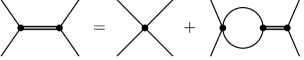
Figure 1.2: The Bethe-Salpeter equation for the meson-propagators in RPA (double line). The solid lines indicate quark propagators.

In the vector channel we proceed in a similar way. The only difference is the the more complicated Lorentz structure of the polarization function and the resulting propagator. Since the polarization function can depend only on one four-momentum, in our notation $q$, its tensor structure is generally given by

$$\Pi_{\rho}^{{\mu\nu},ab}(q)=\delta_{ab}(g^{\mu\nu}f_{1}(q^{2})+\frac{q^{\mu}q^{\nu}}{q^{2}}f_{2}(q^{2}))~{},$$ (1.13)

with two scalar functions $f_{1}$ and $f_{2}$. This can be separated into a tranverse and a longitudinal part using the corresponding projectors,

$$T^{\mu\nu}=-g^{\mu\nu}+\frac{q^{\mu}q^{\nu}}{q^{2}}\quad{\rm and}\quad L^{\mu\nu}=\frac{q^{\mu}q^{\nu}}{q^{2}}~{}.$$ (1.14)

However, because of vector current conservation, the polarization function in the vector channel has to be transverse, i.e.

$$q_{\mu}\,{\Pi}_{\rho}^{\mu\nu,ab}(q)=q_{\nu}\,{\Pi}_{\rho}^{\mu\nu,ab}(q)=0\;.$$ (1.15)

The tranverse structure, together with the assumption of Lorentz invariance, not only simplifies the determination of the tensor structure of the corresponding propagator but also the evaluation of the polarization function itself: With the ansatz

$$\Pi^{{\mu\nu},ab}_{\rho}(q)=T^{\mu\nu}(q)\delta_{ab}\Pi_{\rho}(q)$$ (1.16)

we only need to evaluate the (Lorentz) scalar function

$$\Pi^{ab}_{\rho}(q)=-\frac{1}{3}g_{\mu\nu}\Pi^{{\mu\nu},ab}_{\rho}(q)~{}.$$ (1.17)

Finally one arrives at the following expression for the propagator of the $\rho$-Meson

$$D_{\rho}^{\mu\nu,ab}(q)\;\equiv\;(D_{\rho}(q)\;T^{\mu\nu}+2g_{v}\;L^{{\mu\nu}})\;\delta_{ab}=(\frac{-2g_{v}}{1-2g_{v}\Pi_{\rho}(q)}\,T^{\mu\nu}+2g_{v}\;L^{{\mu\nu}})\;\delta_{ab}~{}.$$ (1.18)

In section 1.5 we will explicitly show that the polarization function in the vector channel is indeed transverse, provided that a suitable regularization procedure is used. In section 2.1 we will discuss a further consequence of vector current conservation, namely that $\Pi_{\rho}(q)$ should vanish for $q^{2}=0$, in the context of the regularization procedure we will apply.

In the same way the propagator of the $a_{1}$-meson can be obtained from the transverse part of the axial polarization function $\Pi_{a_{1}}^{T}(q)\delta_{ab}=-\frac{1}{3}T_{{\mu\nu}}\Pi_{a_{1}}^{{\mu\nu},ab}(q)$. As discussed e.g. in Ref. [49], $\Pi_{a_{1}}^{\mu\nu}$ in addition contains a longitudinal part which contributes to the pion propagator together with the pseudoscalar polarization function $\Pi_{\pi}^{ab}$ and the mixed ones, which contain one pseudoscalar and one axial vertex. There is no conceptual difficulty in dealing with this so-called “$\pi$-$a_{1}$-mixing”. We will neglect it in the following discussion, and only consider the pseudoscalar part of the pion propagator, in order to keep the formalism as simple as possible. The pion propagator including $\pi$-$a_{1}$-mixing is discussed in App. C.1.

It follows from Eqs. (1.11) to (1.18) that the functions $D_{M}(q)$ are of order $1/N_{c}$. The explicit form of these functions can be found in App. B. We will call them “propagators” although strictly speaking they have to be interpreted as the product of a meson propagator with a meson-quark coupling constant squared. The latter is given by the inverse of the residue of the function $D_{M}(q)$ at the pole, whereas the mass of the corresponding meson is determined by the location of the pole,

$$D_{M}^{-1}(q)|_{q^{2}=m_{M}^{2(0)}}=0\;,\qquad g_{Mqq}^{-2(0)}=\frac{d\Pi_{M}(q)}{dq^{2}}|_{q^{2}=m_{M}^{2(0)}}\;.$$ (1.19)

The superscript $(0)$ here serves to indicate that $m_{M}^{2(0)}$ and $g_{Mqq}^{(0)}$ are RPA quantities. In a $1/N_{c}$-expansion these quantities are of leading order. One can easily convince oneself that they are of order ${\mathcal{O}}(1)$ and $1/\sqrt{N_{c}}$, respectively. Dealing with $\pi$-$a_{1}$-mixing, we have only to keep in mind that in addition to a pseudoscalar pion-quark coupling constant an axial one exists. This will be discussed in App. C.1.

1.3 Extensions of the standard approximation

The Hartree + RPA (only direct contributions) scheme, which was discussed in the previous section is consistent with chiral symmetry. This means, for instance, that a spontaneously broken symmetry enforces the existence of massless Goldstone bosons. Within that approximation scheme also the validity of the Goldberger-Treiman and the Gell-Mann–Oakes–Renner relation, which determines the behavior of the pion mass if the symmetry is explicitly broken due to a small current quark mass $m_{0}$, can be shown [16, 17, 18]. We will present a proof for these relations in section 1.4.1. Since chiral symmetry is one of the main features of the NJL model, any approximation should be consistent with chiral symmetry. Within this section we will discuss different approximation schemes which have in common that on the one hand they fulfill the requirements of chiral symmetry and on the other hand they go beyond the standard Hartree + RPA scheme. We will begin with a strict $1/N_{c}$-expansion up to next-to-leading order, proceed by discussing the “$\Phi$-derivable method” and then consider a one-loop expansion of the effective action. The latter corresponds to a selfconsistent extension of the gap equation including a meson-loop term. These methods enable us to include mesonic fluctuations in our investigations.

1.3.1 $1/N_{c}$-expansion

Within this section we will consider the quark self-energy and the polarization functions of the mesons in a $1/N_{c}$-expansion up to next-to-leading order. To determine the corresponding correction terms let us first recall the $1/N_{c}$-counting rules for the leading-order quantities: Quark propagators are of order unity whereas the meson propagators are of order $1/N_{c}$. In addition one has to keep in mind that, because of the trace in color space, every quark loop contributes a factor $N_{c}$ and every four-fermion vertex a factor $1/N_{c}$ due to the order of the coupling constant.

For the quark self-energy we find two correction terms,

$$\delta\Sigma(p)=\delta\Sigma^{(a)}+\delta\Sigma^{(b)}(p)\;.$$ (1.20)

These terms are graphically shown in Fig. 1.3. A solid line corresponds here to a quark propagator in Hartree approximation (${\cal O}(1)$) and a double line to an RPA meson propagator (${\cal O}(1/N_{c})$). With the help of the above mentioned counting rules it is then easy to convince oneself that these are indeed the only correction terms to the quark self-energy in next-to-leading order. Any further contribution inevitably contains in addition at least one quark loop and two coupling constants or one meson propagator, which leads altogether to an additional factor $1/N_{c}$.

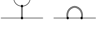
Figure 1.3: The $1/N_{c}$-correction terms $\delta\Sigma^{(a)}$ (left) and $\delta\Sigma^{(b)}$ (right) to the quark self-energy.

The correction terms to the quark self-energy determine those to the quark propagator to order $1/N_{c}$,

$$\delta S(p)=S(p)\,\delta\Sigma(p)\,S(p)~{}.$$ (1.21)

$S(p)$ here denotes the quark propagator in Hartree approximation. In leading order the self-energy has been iterated in order to obtain the corresponding propagator. This has been done via the selfconsistent solution of the gap equation, Eq. (1.2). However, in next-to-leading order an iteration of the self-energy would lead to terms of arbitrary order in $1/N_{c}$ in the propagator. Following Eq. (1.5) the correction to the quark condensate is given by

$$\delta\langle{\bar{\psi}\psi}\rangle=-i\int\frac{d^{4}p}{(2\pi)^{4}}\;{\mbox{\rm Tr}}\,\delta S(p)\;.$$ (1.22)

We find four correction terms, $\delta\Pi_{M}^{(a)}$ to $\delta\Pi_{M}^{(d)}$, to the meson polarization functions. These are displayed in Fig. 1.4 together with the leading order contribution. Solid lines denote again quark propagators, double lines RPA meson propagators. This leads to the following form of the complete polarization function:

$${\tilde{\Pi}}_{M}(q)=\Pi_{M}(q)+\sum_{k=a,b,c,d}\;\delta\Pi_{M}^{(k)}(q)\;.$$ (1.23)

The correction terms, which contain either one RPA propagator and one quark loop or two RPA propagators and two quark loops, are of order unity, whereas the leading-order term is of order $N_{c}$.

The meson propagators are again, similar to the leading order, given as solution of a Bethe-Salpeter equation. The only difference to the propagators in RPA consists of taking into account the polarization functions up to next-to-leading order. Thus we arrive at the following expressions for the meson propagators, analogously to Eqs. (1.12) and (1.18),

$${\tilde{D}}_{M}(q)=\frac{-2g_{M}}{1-2g_{M}{\tilde{\Pi}}_{M}(q)}\;.$$ (1.24)

We should remark that these meson propagators contain arbitrary orders in $1/N_{c}$ although we have determined the polarization functions by a strict expansion in powers of $1/N_{c}$. This is due to the iteration of the product of the polarization functions with the corresponding coupling constant.

This remark similarly concerns the meson masses. These are defined, in analogy to Eq. (1.19), as the location of the pole of the propagator,

$$\tilde{D}_{M}^{-1}(q)|_{q^{2}=m_{M}^{2}}=0\;.$$ (1.25)

Because of the implicit definition, $m_{M}$ also contains terms of arbritrary orders in $1/N_{c}$. This definition is consistent with the Goldstone theorem, but in the context of the Gell-Mann–Oakes–Renner relation we will encounter difficulties caused by higher-order (beyond next-to-leading order) contributions to the pion mass. This point will be discussed in detail in section 1.4.3.

For the evaluation of the various contributions it is convenient to introduce effective meson-meson vertices which consist of quark loops. We need two different types of meson-meson vertices, a three-meson vertex, containing a quark triangle, shown on the l.h.s. of Fig. 1.5 and a four-meson vertex, containing a quark box, shown on the r.h.s. of Fig. 1.5. For external mesons $M_{1}$, $M_{2}$ and $M_{3}$ the quark triangle has the following form:

$$-i\Gamma_{M_{1},M_{2},M_{3}}(q,p) = -\int\frac{d^{4}k}{(2\pi)^{4}}\Big{\{}{\mbox{\rm Tr}}\,[\Gamma_{M_{1}}iS(k)\Gamma_{M_{2}}iS(k-p)\Gamma_{M_{3}}iS(k+q)]$$ (1.26)

$$\hskip 52.63777pt+{\mbox{\rm Tr}}\,[\Gamma_{M_{1}}iS(k-q)\Gamma_{M_{3}}iS(k+p)\Gamma_{M_{2}}iS(k)]\Big{\}}~{}.$$

The operators $\Gamma_{M}$ have already been defined below Eq. (1.2). The above expression already contains a sum over both possible orientations of the quark loop.

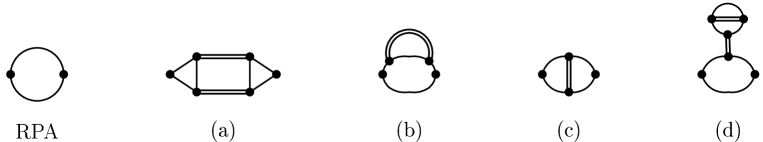
Figure 1.4: Contributions to the meson polarization functions in leading (RPA) and next-to-leading order in $1/N_{c}$.

The four-meson vertices can be written in the following way:

$$-i\Gamma_{M_{1},M_{2},M_{3},M_{4}}(p_{1},p_{2},p_{3})\phantom{\int\frac{d^{4}k}{(2\pi)^{4}}}$$

$$=-\int\frac{d^{4}k}{(2\pi)^{4}}\Big{(}{\mbox{\rm Tr}}\,[\Gamma_{M_{1}}iS(k)\Gamma_{M_{2}}iS(k-p_{2})\Gamma_{M_{3}}iS(k-p_{2}-p_{3})\Gamma_{M_{4}}iS(k+p_{1})]$$

$$\phantom{=\int\frac{d^{4}k}{(2\pi)^{4}}\Big{(}}+{\mbox{\rm Tr}}\,[\Gamma_{M_{1}}iS(k-p_{1})\Gamma_{M_{4}}iS(k+p_{2}+p_{3})\Gamma_{M_{3}}iS(k+p_{2})\Gamma_{M_{2}}iS(k)]\Big{)}~{}.$$ (1.27)

Here again we have summed over both possible orientations of the quark loop.

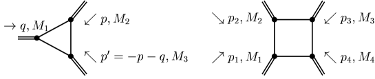
Figure 1.5: Quark triangle $-i\Gamma_{M_{1},M_{2},M_{3}}(q,p)$ (left) and quark box $-i\Gamma_{M_{1},M_{2},M_{3},M_{4}}(p_{1},p_{2},p_{3})$ (right).

With the help of the above definitions the $1/N_{c}$-correction terms to the quark self-energy as well as to the meson polarization functions can be written in a relatively compact form. For the momentum independent contribution $\delta\Sigma^{(a)}$ to the quark self-energy we obtain

$$\delta\Sigma^{(a)}=-\frac{1}{2}D_{\sigma}(0)\;\sum_{M}\;\int\frac{d^{4}p}{(2\pi)^{4}}\;D_{M}(p)\,\Gamma_{M,M,\sigma}(p,-p)=D_{\sigma}(0)\,\Delta\;.$$ (1.28)

Here we have introduced the constant $\Delta$,

$$\Delta=\frac{1}{2}\int\frac{d^{4}p}{(2\pi)^{4}}\sum_{M}(-iD_{M}(p))(-i\Gamma_{M,M,\sigma}(p,-p))~{},$$ (1.29)

which we will need later on for instance for the evaluation of diagram $\delta\Pi_{M}^{(d)}$. The factor $1/2$ in the definition of $\Delta$ is a symmetry factor, which is necessary in order to avoid double counting which otherwise would arise from the sum over both possible orientations of the quark loop in the definition of quark triangle, Eq. (1.26). $\Delta$ consists of a quark triangle coupling to a meson loop and an external scalar coupling. In principle we should have allowed also for other external couplings, for instance a pseudoscalar one, and sum over all these couplings and the corresponding meson propagators in Eq. (1.28). It turns out, however, that only the scalar coupling leads to a nonvanishing contribution to $\Delta$ because $\Gamma_{M,M,M_{1}}(p,-p)=0$ for $M_{1}\neq\sigma$ (cf. App. D).

For the momentum dependent correction term $\delta\Sigma^{(b)}$ to the quark self-energy we arrive at the following expression:

$$\delta\Sigma^{(b)}(k)=i\sum_{M}\;\int\frac{d^{4}p}{(2\pi)^{4}}\;D_{M}(p)\;\Gamma_{M}\,S(k-p)\,\Gamma_{M}\;.$$ (1.30)

The $1/N_{c}$-correction to the quark condensate is closely related to the quark self-energy (cf. Eqs. (1.5) and (1.22)). Inserting the expressions for $\delta\Sigma^{(a)}$ and $\delta\Sigma^{(b)}$ into Eq. (1.21), and performing the trace in Eq. (1.22) we obtain

$$\delta\langle{\bar{\psi}\psi}\rangle=-\Delta\Pi_{\sigma}(0)D_{\sigma}(0)+\Delta~{}.$$ (1.31)

This expression can be further simplified with the help of the definition of the RPA propagator $D_{\sigma}$ in terms of the corresponding polarization function $\Pi_{\sigma}$, cf. Eq. (1.12). We finally obtain for the $1/N_{c}$-correction to the quark condensate

$$\delta\langle{\bar{\psi}\psi}\rangle=-\frac{D_{\sigma}(0)\,\Delta}{2g_{s}}\;.$$ (1.32)

The evaluation of the various contributions to the polarization functions give

$$\delta\Pi^{(a)}_{M}(q) = \phantom{-}\frac{i}{2}\int\frac{d^{4}p}{(2\pi)^{4}}\sum_{M_{1}M_{2}}\Gamma_{M,M_{1},M_{2}}(q,p)\,D_{M_{1}}(p)\,\Gamma_{M,M_{1},M_{2}}(-q,-p)\,D_{M_{2}}(-p-q)\;,$$

$$\delta\Pi^{(b)}_{M}(q) = -i\,\int\frac{d^{4}p}{(2\pi)^{4}}\hskip 8.53581pt\sum_{M_{1}}\;\Gamma_{M,M_{1},M_{1},M}(q,p,-p)\,D_{M_{1}}(p)\;,$$

$$\delta\Pi^{(c)}_{M}(q) = -\frac{i}{2}\int\frac{d^{4}p}{(2\pi)^{4}}\hskip 7.11317pt\sum_{M_{1}}\;\Gamma_{M,M_{1},M,M_{1}}(q,p,-q)\,D_{M_{1}}(p)\;,$$

$$\delta\Pi^{(d)}_{M}(q) = \frac{i}{2}\;\Gamma_{M,M,\sigma}(q,-q)\,D_{\sigma}(0)\;\int\frac{d^{4}p}{(2\pi)^{4}}\hskip 8.53581pt\sum_{M_{1}}\;\Gamma_{M_{1},M_{1},\sigma}(p,-p)\,D_{M_{1}}(p)\;,$$ (1.33)

$$= -i\,\Gamma_{M,M,\sigma}(q,-q)\,D_{\sigma}(0)\,\Delta\;.$$

The symmetry factor $1/2$ in $\delta\Pi^{(c)}_{M}$ and $\delta\Pi^{(d)}_{M}$ has been introduced for the same reason as the factor $1/2$ in Eq. (1.28). In $\delta\Pi^{(a)}_{M}$ it is necessary in order to account for the fact that the exchange of $M_{1}$ and $M_{2}$ leads to the same diagram.

For the further evaluation of Eqs. (1.28) to (1.33) we will proceed in two steps. First the quark loops for the RPA meson propagators and the effective three- and four-meson vertices will be calculated and then we will evaluate the remaining meson loops.

In principle the sum in Eqs. (1.28) to (1.33) is over all possible intermediate states, i.e. $\sigma$-,$\pi$-,$\rho-$ and $a_{1}$-mesons. However, pions, the lightest particles in the system, are expected to yield the dominant contribution to most applications. For instance, the behavior of the quark condensate at low temperatures is mainly driven by thermally excited pions. The $\rho$-meson spectral function is also primarily determined by a two-pion intermediate state. Other possible contributions to $\delta\Pi^{(a)}$, like $\pi a_{1}$-, $\rho\sigma$-, $\rho\rho$- or $a_{1}a_{1}$- intermediate states are expected to be much less important since the corresponding decay channels open far above the $\rho$-meson mass. In principle we have to keep in mind that the physical $a_{1}$ as well as the $\rho$ are broad resonances which principally couple to three- and two-pion intermediate states, respectively. Therefore the physical threshold for the decay of the $\rho$ into $\pi a_{1}$ or $\rho\rho$ lies at $4m_{\pi}\sim 560$ MeV, i.e. below the $\rho$-meson mass of about 770 MeV. But of course considerable contributions will arise only above $2m_{\rho}\approx 1.6$ GeV and $m_{a_{1}}+m_{\pi}\approx 1.4$ GeV. Besides, experimentally the contribution of these intermediate states is negligible anyway, one finds that the branching ratio of $\rho\rightarrow\pi\pi$ is about 100% [50].

From a phenomenological point of view it therefore seems well justified to consider only pionic intermediate states. However, consistency with chiral symmetry requires that also scalar states are considered, whereas vector and axial intermediate states can be neglected without any difficulties. Since the evaluation of the various contributions can be simplified considerably by neglecting vector and axial intermediate states we will exclusively take scalar and pseudoscalar intermediate states into account for most of the calculations. To describe a $\rho$-meson we have certainly to allow for an external vector coupling in the diagrams shown in Fig. 1.4.

Another point which complicates the treatment of vector and axial intermediate states is that they cause strong divergencies in the correction terms to the polarization functions. On the one hand this has certainly to be attributed to the non-renormalizability of the NJL model, on the other hand it is related to a rather fundamental problem concerning the regularization of the RPA vector and axial polarization function. This will be discussed in more detail in section 2.1 and section 2.4.3, respectively.

1.3.2 $\Phi$-derivable theory

The main disadvantage of the approximation discussed in the previous section is that the $1/N_{c}$-correction terms are treated perturbatively. For instance, though we have considered corrections to the quark self-energy, these have not been taken into account in the gap equation. Consequently all quark propagators contributing to the $1/N_{c}$-corrected polarization functions are determined in Hartree approximation. As long as the $1/N_{c}$-correction terms are small compared with the leading-order contributions this approach seems reasonable. But a description of the chiral phase transition will certainly not be possible within that scheme.

An approach which treats the mesons selfconsistently is highly desirable, since e.g. the thresholds for the decay $\rho\rightarrow\pi a_{1}$ would then be located at $4m_{\pi}$, but this is a very difficult task. For this reason we will be content with a scheme which enables us at least to treat the quarks selfconsistently. In the literature two functional methods can be found which, in principle, allow to construct a selfconsistent scheme which is consistent with chiral symmetry. One is the so-called “$\Phi$-derivable”-method [37, 38], the other an expansion of the “effective action” [51, 52]. The latter will be discussed in the next section. We will begin here by illustrating the $\Phi$-derivable method on the Hartree + RPA scheme which emerges as the first approximation. Subsequently we will go one step further which will generate a non-local contribution to the gap equation.

The starting point of a $\Phi$-derivable theory is a functional $\Phi$, which in principle contains all two-particle-irreducible skeleton diagrams which can be constructed from the interactions and fields of the underlying Lagrangian. Two-particle-irreducible diagrams are those which cannot be split into parts by cutting two lines. In the diagrams all Greens functions have to be full ones. The corresponding self-energies can be obtained by functional derivatives of $\Phi$ with respect to the (full) Greens functions. Generally a symmetry conserving approximation is generated by taking any subset of diagrams [38]. The thermodynamic potential per volume, $\Omega$, which is identical to the energy density of the system in vacuum, can be expressed as follows with the help of the functional $\Phi$,

$$\Omega=-iTr\ln(i\;S^{-1})+Tr(\Sigma\,iS)+\Phi(S)~{},$$ (1.34)

where $S^{-1}=S_{0}^{-1}+\Sigma$ represents the full Greens function, i.e. in our case the full quark propagator. The symbol $Tr$ denotes here a trace over internal degrees of freedom, such as color-, spin- or isospin degrees of freedom, as well as an integral over momentum or coordinate space. For instance, in vacuum we have

$$Tr(\Sigma S)\equiv\int\frac{d^{4}p}{(2\pi)^{4}}{\mbox{\rm Tr}}(\Sigma(p)S(p))~{}.$$

An expression for the self-energy can be derived by requiring stationarity of $\Omega$ with respect to variations of the full propagator. One finds

$$\Sigma=-\frac{\delta\Phi}{\delta\;(iS)}~{}.$$ (1.35)

Evidently this means that the self-energy is given by the functional derivative of $\Omega$ with respect to the full propagator. The scattering kernel for the Bethe-Salpeter equation is in turn given by the functional derivative of the self-energy with respect to the full propagator,

$$K=\frac{\delta\Sigma}{\delta iS}=-\frac{\delta^{2}\Phi}{\delta\;(iS)\delta\;(iS)}~{}.$$ (1.36)

Let us now begin considering the simplest possible subset of two-particle-irreducible diagrams. In the NJL model this is given by the “glasses”, displayed in Fig. 1.6. Again, solid lines represent quark propagators. The wavy lines have been introduced to visualize the direction of the interaction at the four-point vertices.

Figure 1.6: The “glasses”, simplest contribution to the functional $\Phi$.

To that approximation $\Phi$ is explicitly given by

$$\Phi^{(0)}[S^{(0)}]=-\sum_{M}g_{M}\Big{(}-\int\frac{d^{4}p}{(2\pi)^{4}}{\mbox{\rm Tr}}(\Gamma_{M}\,iS^{(0)}(p))\Big{)}^{2}~{}.$$ (1.37)

The superscript ${(0)}$ again denotes quantities to first approximation. Below we will demonstrate that the above expression for the functional $\Phi$ generates the Hartree + RPA scheme for quarks and mesons, respectively.

According to Eq. (1.35) the quark self-energy is a priori momentum dependent and a matrix in color-, flavor- and Dirac-space. Performing the functional derivative ($i$ and $j$ are multi-indices, referring to color-, flavor- and Dirac-space),

$$\Sigma^{(0)}_{ij}(q_{1},q_{2}) \equiv \delta(q_{1}+q_{2})\Sigma^{(0)}_{ij}=\int d^{4}x_{1}{\mathrm{e}}^{-iq_{1}\cdot x_{1}}\int d^{4}x_{2}{\mathrm{e}}^{-iq_{2}\cdot x_{2}}\frac{\delta\Phi^{(0)}[S^{(0)}]}{\delta\;(iS^{(0)}_{ij}(x_{1},x_{2}))}$$ (1.38)

$$= \delta(q_{1}+q_{2})\sum_{M}2ig_{M}\Gamma_{M,ji}\int\frac{d^{4}p}{(2\pi)^{4}}{\mbox{\rm Tr}}(\Gamma_{M}S^{(0)}(p))~{},$$

we find, however, that the self-energy is at least momentum independent. Remembering that only the scalar channel leads to a nonvanishing contribution we conclude that it is in addition proportional to unity in all spaces. After a comparison of the resulting expression for the self-energy with the gap equation, Eq. (1.2), it becomes obvious that $\Sigma^{(0)}_{ij}$ is identical to the Hartree self-energy $\Sigma_{H}$ derived in section 1.2.

For the scattering kernel $K^{(0)}$ we obtain

$$K^{(0)}_{ij,kl}(q_{1},q_{2},q_{3},q_{4}) = \int d^{4}x_{1}\int d^{4}x_{2}\int d^{4}x_{3}\int d^{4}x_{4}{\mathrm{e}}^{-i(q_{1}\cdot x_{1}+q_{2}\cdot x_{2}+q_{3}\cdot x_{3}+q_{4}\cdot x_{4})}\begin{array}[]{c}\frac{\delta\Sigma^{(0)}_{ij}(x_{1},x_{2})}{\delta\;(iS^{(0)}_{kl}(x_{3},x_{4}))}\end{array}$$ (1.40)

$$= \sum_{M}2g_{M}\Gamma_{M,ji}\Gamma_{M,lk}\delta(q_{1}+q_{2}+q_{3}+q_{4})~{}.$$ (1.41)

As can be seen from a comparison with Eq. (1.8) this expression meets our expectations: It is indeed the scattering kernel for the $T$-matrix in RPA. We therefore conclude that the Hartree + RPA approximation scheme can be derived within the $\Phi$-derivable method, if the functional $\Phi$ is restricted to the “glasses”.

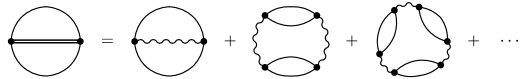
Figure 1.7: The “ ring sum”, contribution to the functional $\Phi$.

A suggestive extension for $\Phi$ is to take also the “ring sum”, visualized in Fig. 1.7, into account. Evaluating the diagrams, “glasses” and ring sum, we arrive at the following expression for $\Phi$:

$$\Phi[S] = -\sum_{M}g_{M}\Big{(}-\int\frac{d^{4}p}{(2\pi)^{4}}{\mbox{\rm Tr}}(\Gamma_{M}\,iS(p))\Big{)}^{2}$$ (1.42)

$$-\frac{i}{2}\int\frac{d^{4}p}{(2\pi)^{4}}\{\ln(1-2g_{s}\Pi_{\sigma}(p))+3\ln(1-2g_{s}\Pi_{\pi}(p))\}~{}.$$

The functions $\Pi_{M}(p)$ were defined in Eq. (1.11). We have to keep in mind that $S$ here denotes a full propagator and not a propagator in Hartree approximation as it originally appeared in the definition of $\Pi_{M}$ in Eq. (1.11). Proceeding in the same way as above (cf. Eq. (1.38)) we obtain for the quark self-energy, $\Sigma_{ij}(q_{1},q_{2})=\delta(q_{1}+q_{2})\Sigma_{ij}(q_{1})$,

$$\Sigma_{ij}(q_{1})=\Sigma_{H,ij}+\delta\Sigma^{(b)}_{ij}(q_{1})~{}.$$ (1.43)

$\delta\Sigma^{(b)}(q)$ was defined in Eq. (1.30). The same remark of caution as above concerning the quark propagator $S$ is in order here: The expressions on the r.h.s. of Eq. (1.43) have to be evaluated with the full propagator. The upper panel of Fig. 1.8 displays the corresponding gap equation. Here solid lines stand for quark propagators as they emerge from the selfconsistent solution of Eq. (1.43).

To determine the scattering kernel for the Bethe-Salpeter equation which describes the mesons, the analogous procedure leading to Eq. (1.41) is applied. One finds

$$K_{ij,kl}(q_{1},q_{2},q_{3},q_{4}) = \delta(q_{1}+q_{2}+q_{3}+q_{4})\Big{\{}\sum_{M}2g_{M}\Gamma_{M,ji}\Gamma_{M,lk}+D_{M}(q_{1}+q_{4})\Gamma_{M,li}\Gamma_{M,jk}$$ (1.44)

$$+2\;i\;\int\frac{d^{4}k}{(2\pi)^{4}}D_{M}(k+q_{3})D_{M}(k-q_{4})(\Gamma_{M}iS(k-q_{1}-q_{4})\Gamma_{M})_{ji}(\Gamma_{M}iS(k)\Gamma_{M})_{kl}\Big{\}}~{}.$$

The corresponding Bethe-Salpeter equation for the quark-antiquark $T$-matrix is displayed in the lower part of Fig. 1.8. In Ref. [42] this representation of the $T$-matrix was generated graphically by coupling an external current to each quark line in the corresponding gap equation, which is shown in the upper part of Fig. 1.8. Moreover, with the help of axial Ward identities one can show generally the existence of a pole in $T$ for $(q_{1}+q_{2})^{2}=0$.

Because of the non-trivial momentum dependence of the self-energy it is a very difficult task to obtain an explicit solution of the gap equation, Eq. (1.43). Therefore we will put this scheme aside and concentrate in explicit calculations on the expansion of the effective action which leads to a local contribution to the gap equation and is much easier to handle. This will be discussed in the next section.

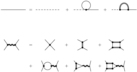
Figure 1.8: (upper panel) Gap equation as it results from $\Phi$ if the ring sum is included, (lower panel) corresponding quark-antiquark scattering matrix.

1.3.3 One-meson-loop expansion of the effective action

The scheme we will derive within this section was first discussed by Dmitrašinović et al. [29]. The authors started from a gap equation which in addition to the Hartree self-energy contains a local meson-loop contribution. They found a consistent scheme to describe mesons and proved various relations following from chiral symmetry explicitly , like e.g. the Goldstone theorem. The same scheme was later derived more systematically by Nikolov et al. [30] using the effective action formalism. Here we will follow the method of that reference. Let us begin with a derivation of an expression for the effective action. We will mainly follow the presentation of Ref. [36], Chapter 16. The interested reader is referred to that reference for further details. The starting point is a theory with an action $I[\phi]$. Throughout the derivation we will, for simplicity, only regard a theory with a scalar field $\phi$, which couples to an external classical source $j$. The generating functional $W[j]$ is then given in path integral representation by

$${\mathrm{e}}^{iW[j]}=\int{\mathcal{D}}(\phi)\exp\Big{(}iI[\phi]+i\int d^{4}x\phi(x)j(x)\Big{)}$$ (1.45)

The functional $W[j]$ contains all connected vacuum diagrams, which can be constructed from the underlying theory in the presence of the source $j$. The vacuum expectation value of the fields $\phi$ can be obtained from a derivative of $W[j]$ with respect to the external source $j$

$$\langle{\phi(x)}\rangle=\frac{\delta W[j]}{\delta j(x)}\Big{|}_{j=0}~{}.$$ (1.46)

This expectation value can in general also be defined in the presence of the source, we will call it $\varphi_{J}$,

$$\varphi_{J}(x)=\frac{\delta W[j]}{\delta j(x)}\Big{|}_{j=J}~{}.$$ (1.47)

For a given $\varphi_{J}$ this equation can in principle be solved for $J$. Throughout the following derivation we will denote the current, which is related to $\varphi_{J}$ via Eq. (1.47), by $J$. A functional $\Gamma[\varphi_{J}]$, which no longer depends on $j$ but on $\varphi_{J}$, can be obtained from $W[j]$ by performing a Legendre transform,

$$\Gamma[\varphi_{J}]=W[J]-\int d^{4}x\varphi_{J}(x)J(x)~{}.$$ (1.48)

This functional $\Gamma[\varphi_{J}]$ is called “effective action”. It contains all one-particle-irreducible diagrams (in the presence of the source) of the theory [36]. Similarly to two-particle-irreducible diagrams, one-particle-irreducible ones are those which cannot be split into parts by cutting one line. One important property of $\Gamma$ can be derived from the derivative with respect to $\varphi_{J}$,

$$\frac{\delta\Gamma[\varphi_{J}]}{\delta\varphi_{J}(y)} = \int d^{4}x\frac{\delta W[j]}{\delta j(x)}\frac{\delta j(x)}{\delta\varphi_{j}(y)}\Big{|}_{j=J}-\int d^{4}x\varphi_{J}(x)\frac{\delta J(x)}{\delta\varphi(y)}-J(y)$$ (1.49)

$$= -J(y)~{}.$$

Hence, if the source $J$ vanishes, only the fields $\varphi_{S}$ at the stationary points of $\Gamma[\varphi_{J}]$,

$$\frac{\delta\Gamma[\varphi_{J}]}{\delta\varphi_{J}(y)}\Big{|}_{\varphi=\varphi^{S}}=0~{},$$ (1.50)

are possible fields $\varphi_{J}$. This means in particular that the vacuum expectation values of the field $\phi$ are given as the values of $\varphi_{J}$ at the stationary points of $\Gamma$, i.e. $\varphi^{S}=\langle{\phi}\rangle$. From this point of view the field $\varphi_{J}$ behaves similarly to a classical field whose equations of motion can be generated from the stationarity condition of the action $I[\phi]$. Thus the effective action can be regarded as some sort of “action with quantum fluctuations”.

Propagators can be obtained from the second derivative of $W[j]$ with respect to the source,

$$\Delta(x,y)=\langle{\Phi(x)\Phi(y)}\rangle=\frac{\delta^{2}W[j]}{\delta j(x)\delta j(y)}\Big{|}_{j=0}=\frac{\delta\varphi_{J}(x)}{\delta j(y)}\Big{|}_{j=0}~{}.$$ (1.51)

This can also be derived from the effective action,

$$\frac{\delta^{2}\Gamma[\varphi]}{\delta\varphi(x)\delta\varphi(y)}\Big{|}_{\varphi=\varphi^{S}}=\frac{\delta j(x)}{\delta\varphi_{j}(y)}\Big{|}_{j=0}=\Delta(x,y)^{-1}~{}.$$ (1.52)

It is convenient to introduce another quantity, the effective potential. Let us assume that we wish to calculate the effective action $\Gamma[\varphi]$ with constant, i.e. space-time-independent, fields $\varphi(x)\equiv\varphi_{0}$. Then $\Gamma[\varphi]$ will be proportional to the volume of space-time ${\mathcal{V}}_{4}=\int d^{4}x$. Therefore we can write the effective action in the form

$$\Gamma[\varphi]=-{\mathcal{V}}_{4}V(\varphi_{0})~{},$$ (1.53)

where $V(\varphi_{0})$ is not a functional of $\varphi$ but an ordinary function. This function is known as the effective potential [53]. The effective potential can be interpreted in terms of the energy density [36]. $V(\varphi_{0})$ can be interpreted as the minimum of the energy density for all states with expectation values $\varphi$ for the fields $\phi$.

After having explained some general aspects of the effective action let us now come to the determination of an explicit expression for $\Gamma[\varphi]$. Certainly it will be impossible to obtain an exact result for the effective action in an interacting theory because the path integral in Eq. (1.48) can in general not be carried out. This is only possible for constant, linear or quadratic terms. Thus, expanding the argument of the exponential in Eq. (1.45) around some fixed field $\varphi_{0}(x)$ which satisfies

$$\frac{\delta I[\phi]}{\delta\phi}\Big{|}_{\phi=\varphi_{0}}=-j$$ (1.54)

up to quadratic terms in the fields, we can evaluate the path integral and arrive at an expression for the effective action $\Gamma[\varphi_{0}]$ up to “one-loop” (see [36], Chapter 16),

$$i\;\Gamma^{(1)}[\varphi]=iI[\varphi]+\frac{1}{2}Tr\ln\Big{(}i\frac{\delta^{2}I[\varphi]}{\delta\varphi\delta\varphi}\Big{)}~{}.$$ (1.55)

The first term in Eq. (1.55) is the “zero-loop” or “tree-level”, the second one the “one-loop” contribution. Strictly speaking the field $\varphi$ which arises from the Legendre transform in Eq. (1.48) not necessarily needs to coincide with $\varphi_{0}$ which has been introduced for the evaluation of the path integral. However, at tree-level it is obvious that both fields are identical. Besides, it can be shown that in a perturbative expansion this is true up to one-loop order [54].

It can be shown (see e.g. [36]) that in most cases the effective action $\Gamma[\varphi]$ has the same symmetries as the action $I[\phi]$. Especially symmetries which are related to linear transformations of the fields are conserved. This has an important consequence (see e.g. [36, 55]): One can show that a spontaneously broken continuous symmetry then generates a pole at $q^{2}=0$ in the two-point function $\Delta(q)$. This corresponds to the existence of a Goldstone boson.

We are now in a position to apply the effective action formalism to the NJL model. A detailed discussion can be found in Ref. [55]. We will begin our presentation with the lowest-order contribution, i.e. the tree-level approximation which will turn out to be equivalent to Hartree approximation + RPA.

In the remaining part of this section we will drop the vector and axial vector interaction and start from a Lagrangian which contains only scalar and pseudoscalar interaction terms, i. e.

$${\cal L}\;=\;\bar{\psi}(i\partial{\hskip-5.69054pt}/-m_{0})\psi\;+\;g_{s}\,[(\bar{\psi}\psi)^{2}+(\bar{\psi}i\gamma_{5}{\vec{\tau}}\psi)^{2}]\,.$$ (1.56)

The generating functional of the system can be expressed in terms of the path integral

$$Z[\eta,\bar{\eta}]=e^{iW[\eta,\bar{\eta}]}=\int{\mathcal{D}}(\bar{\psi}){\mathcal{D}}(\psi)e^{iI[\bar{\psi},\psi]+i\int d^{4}x(\bar{\psi}(x)\eta(x)+\bar{\eta}(x)\psi(x))}~{},$$ (1.57)

with the action

$$I[\bar{\psi},\psi]=\int d^{4}x{\cal L}(x)~{}.$$ (1.58)

To further proceed it is convenient to “bosonize” the action. This is achieved by introducing auxiliary hermitian fields $\Phi_{a}^{\prime},a=\{0,1,2,3\}$. These collective bosonic fields are chosen in such a way that the action becomes bilinear in the quark fields, i. e.

$$Z[\eta,\bar{\eta}] = \int{\mathcal{D}}(\bar{\psi}){\mathcal{D}}(\psi){\mathcal{D}}(\Phi_{a}^{\prime})\exp\Big{\{}iI(\bar{\psi},\psi)+i\int d^{4}x(\bar{\psi}(x)\eta(x)+\bar{\eta}(x)\psi(x))$$ (1.59)

$$\hskip 56.9055pt-\frac{i}{4g_{s}}\int d^{4}x(\Phi_{a}^{\prime}+2g_{s}\bar{\psi}\Gamma_{a}\psi)^{2}\Big{\}}~{},$$

with $\Gamma_{a}=(1,i\gamma_{5}\vec{\tau})$. The quark fields can now be integrated out. After performing a shift of the auxiliary fields, $\Phi_{a}=\Phi^{\prime}_{a}+(m_{0},\vec{0})$, one finally arrives at the bosonized form of the generating functional

$$Z[\eta,\bar{\eta}]=\int{\mathcal{D}}(\Phi_{a})\exp\Big{\{}iI[\Phi_{a}]+i\int d^{4}x\int d^{4}y\bar{\eta}(y)\,{\mathrm{D}}^{-1}(y,x)\eta(x)\Big{\}}$$ (1.60)

with the action

$$I[\Phi]=-i\;Tr\ln i{\mathrm{D}}-\frac{1}{4g_{s}}\int d^{4}x(\Phi^{2}-2m_{0}\Phi_{0}+m_{0}^{2})~{}.$$ (1.61)

D is the Dirac operator

$${\mathrm{D}}(x,y)=(i\partial\!\!\!/-\Gamma_{a}\Phi_{a})\delta(x-y)~{}.$$ (1.62)

This notation should not be confused with the meson propagator $D_{M}(q)$ we introduced earlier. The first term in Eq. (1.61) arises from the “fermion determinant”. The symbol $Tr$ is therefore to be understood as a functional trace and a trace over internal degrees of freedom such as flavor, color and spin. This is the quark-loop contribution. Expanding the fields around some constant field $\Phi_{a}=(M,\vec{0})+\Delta\Phi_{a}$ we can rewrite the Dirac operator as follows

$${\mathrm{D}}(x,y) = (i\partial\!\!\!/-M)\delta(x-y)-\Gamma_{a}\Delta\Phi_{a}\delta(x-y)$$ (1.63)

$$\equiv {\mathrm{D}_{0}}(x,y)-V~{},$$

where $V$ is of first order in the fluctuations $\Delta\Phi_{a}$. $D_{0}$ corresponds to a quark propagator with “mass” $M$, it can be written as

$$D_{0}(x,y)=\int\frac{d^{4}p}{(2\pi)^{4}}{\mathrm{e}}^{ip\cdot(x-y)}S(p)~{}.$$ (1.64)

The logarithm in the quark-loop term to the action can then be expressed in powers of the fluctuations $\Delta\Phi_{a}$,

$$\ln(i{\mathrm{D}}) = \ln(i{\mathrm{D}_{0}})+\ln(1-{\mathrm{D}_{0}}^{-1}V)$$ (1.65)

$$= \ln(i{\mathrm{D}_{0}})-\sum_{n=1}^{\infty}\frac{({\mathrm{D}_{0}}^{-1}V)^{n}}{n}~{}.$$

This expression will be helpful when we determine the derivatives of the action $I$ with respect to the fields $\Phi$. In which way are the expectation values of the auxiliary fields $\Phi$ related to physical quantities we are interested in? This can most directly be seen for the quark condensate: It can be expressed via the expectation value of $\Phi_{0}$ as

$$\langle{\bar{\psi}\psi}\rangle=\frac{\partial W}{\partial m_{0}}=-\frac{1}{2g_{s}}(\langle{\Phi_{0}}\rangle-m_{0})~{}.$$ (1.66)

From Eq. (1.52) we can infer that the meson propagators can be obtained as second-order derivatives from the effective action. In “zero-loop” approximation the effective action is simply given by,

$$\Gamma^{(0)}[\Phi]=I[\Phi]~{},$$ (1.67)

where we have dropped the fermionic source terms $\eta$ and $\bar{\eta}$ for simplicity. To determine the expectation values of the fields $\Phi$ we first have to build the functional derivative with respect to the fluctuations $\Delta\Phi$. To that end only the first order term in Eq. (1.65) has to be considered. We arrive at the following expression

$$\frac{\delta\Gamma^{(0)}}{\delta\Delta\Phi_{b}(z)}\Big{|}_{\Delta\Phi=0}=\int\frac{d^{4}p}{(2\pi)^{4}}{\mbox{\rm Tr}}[iS(p)\Gamma_{b}]-\frac{1}{2g_{s}}(M-m_{0})\delta_{b0}~{}.$$ (1.68)

Since the trace in the first term on the r.h.s. vanishes for $b\neq 0$ there is no contribution with $b\neq 0$. Comparing the first term on the r.h.s. of the above expression with the definition of the Hartree self-energy we conclude that the expectation value of the fields $\Phi$ in the present approximation can be written in the form $(M,\vec{0})$, where $M$ is given by the solution of the following equation:

$$M-m_{0}-\Sigma_{H}(M)=0~{},$$ (1.69)

with $\Sigma_{H}$ as defined in Eq. (1.2). If we identify the expectation value of the zeroth component of the field $\Phi$, i.e. $M$, with the constituent quark mass $m_{H}$ in Hartree approximation, this equation is identical with the gap equation (Eq. (1.2)). We have to emphasize here that the interpretation of $\langle{\Phi_{0}}\rangle=M$ as a constituent quark mass is not clear a priori. In principle the constituent quark mass should be determined from the pole of the quark propagator. However, in Hartree approximation this pole coincides with $\langle{\Phi_{0}}\rangle$.

If we evaluate the second-order derivative of the effective action $\Gamma^{(0)}$ at the stationary point, we obtain the following result

$$\int d^{4}x_{1}{\mathrm{e}}^{-iq_{1}\cdot x_{1}}\int d^{4}x_{2}{\mathrm{e}}^{-iq_{2}\cdot x_{2}}\frac{\delta^{2}\Gamma^{(0)}}{\delta\Delta\Phi_{a}(x_{1})\Delta\Phi_{b}(x_{2})}\Big{|}_{\Phi=(M,\vec{0})}=\delta(q_{1}+q_{2})\delta_{bc}\Pi_{b}(q_{1})-\frac{\delta(q_{1}+q_{2})\delta_{bc}}{2g_{s}}~{},$$ (1.70)

where we have already exploited the fact that in our case the polarization function $\Pi_{M}$ is diagonal in flavor space. Thus, comparing this result with the definition of the inverse meson propagators in Eq. (1.52), we conclude that we in this way exactly recover the inverse meson propagators in RPA, cf. Eq. (1.12). This allows us to draw the conclusion that the effective action formalism in “zero-loop” approximation yields the same results as the Hartree approximation + RPA.

Extending the effective action to “one-loop”, starting from a bosonized version of the NJL model, means that we take into account mesonic fluctuations. The effective action is then given by Eq. (1.55). The second term in Eq. (1.55) contains the mesonic fluctuations. As discussed in Ref. [55] the method is only meaningful if the second-order functional derivative which enters into this term is positive definite. Otherwise severe problems arise due to an ill-defined logarithm, which would then be complex. We will come back to this point in section 2.3.

Although we introduced this approximation rather generally as “one-loop” approximation we will throughout this work adopt the notation of Ref. [30] and call this approximation scheme the “one-meson-loop approximation” (MLA). This name is motivated by the fact that one-loop contribution in fact contains mesonic fluctuations due to the preceding bosonization procedure. In addition we have to mention that the ”quark-loop” approximation described above is not really a tree-level approximation which would be suggested by the introduction of $\Gamma^{(0)}$ in Eq. (1.55). In order to arrive at the bosonized form of the action, we have integrated out the quark fields, i.e. the bosonized action in principle contains all quark loops.

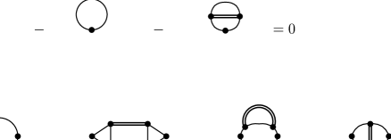
Figure 1.9: The “one-meson-loop approximation scheme”: gap-equation (upper part), and the corresponding mesonic polarization functions (lower part). The double line denotes an RPA meson propagator (see Fig. 1.2), which is selfconsistently constructed from the quark propagators dressed with the local self-energy of the present equation (solid line). The cross stands for the constant term $\langle{\Phi_{0}}\rangle-m_{0}$ in the gap equation (Eq. (1.72)).

For the following derivation of explicit expressions in one-meson-loop approximation it is convenient to first establish relations between the effective meson-vertices introduced in section 1.3.1 and the third- and fourth-order derivative of the action $I[\Phi]$,

$$\int d^{4}x_{1}d^{4}x_{2}d^{4}x_{3}{\mathrm{e}}^{-i(q_{1}\cdot x_{1}+q_{2}\cdot x_{2}+q_{3}\cdot x_{3})}\frac{\delta^{3}I[\Phi]}{\delta(\Phi_{a}(x_{1}))\delta(\Phi_{b}(x_{2}))\delta(\Phi_{c}(x_{3}))}\Big{|}_{\Delta\Phi=0}$$

$$=\delta(q_{1}+q_{2}+q_{3})\Gamma_{a,b,c}(q_{1},q_{2})$$

$$\int d^{4}x_{1}d^{4}x_{2}d^{4}x_{3}d^{4}x_{4}{\mathrm{e}}^{-i(q_{1}\cdot x_{1}+q_{2}\cdot x_{2}+q_{3}\cdot x_{3}+q_{4}\cdot x_{4})}\frac{\delta^{4}I[\Phi]}{\delta(\Phi_{a}(x_{1}))\delta(\Phi_{b}(x_{2}))\delta(\Phi_{c}(x_{3}))\delta(\Phi_{d}(x_{4}))}\Big{|}_{\Delta\Phi=0}$$

$$=-i\delta(q_{1}+q_{2}+q_{3}+q_{4})\Big{(}\Gamma_{a,b,c,d}(q_{1},q_{2},q_{3})+\Gamma_{a,b,d,c}(q_{1},q_{2},q_{4})+\Gamma_{a,c,b,d}(q_{1},q_{3},q_{2})\Big{)}~{}.$$ (1.71)

These relations enable us to straightforwardly derive an equation for the stationary point of the effective action in Eq. (1.55). The following “gap equation” holds [30]:

$$\langle{\Phi_{0}}\rangle-m_{0}-\tilde{\Sigma}(\langle{\Phi_{0}}\rangle)=\langle{\Phi_{0}}\rangle-m_{0}-\Sigma_{H}(\langle{\Phi_{0}}\rangle)-\delta\tilde{\Sigma}(\langle{\Phi_{0}}\rangle)=0~{}.$$ (1.72)

Here $\Sigma_{H}$ is the Hartree contribution to $\langle{\Phi_{0}}\rangle$ as defined in Eq. (1.2). In the upper part of Fig. 1.9 this gap equation is visualized graphically. The cross indicates the constant term $\langle{\Phi_{0}}\rangle-m_{0}$, the second term corresponds to the Hartree contribution and the correction term $\delta\tilde{\Sigma}$ corresponds to the third diagram. It consists of a quark loop dressed by an RPA-meson loop. It can be shown, that at the external vertex only the scalar interaction contributes. Hence $\delta\tilde{\Sigma}$ is given by

$$\delta\tilde{\Sigma}(\langle{\Phi_{0}}\rangle)=-2g_{s}\,\Delta(\langle{\Phi_{0}}\rangle)\;,$$ (1.73)

where $\Delta$ is the constant defined in Eq. (1.29). We should emphasize that these diagrams have to be evaluated selfconsistently at $\langle{\Phi_{0}}\rangle$, which is a solution of Eq. (1.72). Thus all “quark propagators”, also those which enter into the calculation of the RPA meson propagators, have the form $S(p)=(p\!\!\!/-\langle{\Phi_{0}}\rangle)^{-1}$. Because of the new diagram $\delta\tilde{\Sigma}$, these are in general different from the Hartree quark propagators.

We have to comment on the notations we use here. The utilization of the symbol $\Sigma$ for the different contributions and the name “quark propagator” for $S(p)$ suggests that we again, as in the “zero-loop” approximation, deal here with quark self-energies. But as already pointed out, the interpretation of $\langle{\Phi_{0}}\rangle$ as a constituent quark mass should be considered with great care. In the Hartree approximation the expectation value of the field $\Phi_{0}$ is equal to the pole of the quark propagator. Therefore within this approximation, the interpretation of $\langle{\Phi_{0}}\rangle$ as a constituent quark mass is correct. The form of the quark lines which enter the calculations in the MLA seems to point in the same direction. But this is not the case. In Ref. [30] it has already been emphasized that $\langle{\Phi_{0}}\rangle$ is not equal to the pole of the “real” quark propagator. This will become clearer if we look at the quark condensate. If we take $S(p)$ being a quark propagator literally, we expect to obtain the quark condensate by evaluating Eq. (1.5) with the “quark propagator” $S(p)$,

$$\langle{\bar{\psi}\psi}\rangle=-\frac{\Sigma_{H}(\langle{\Phi_{0}}\rangle)}{2g_{s}}=-\frac{\langle{\Phi_{0}}\rangle-m_{0}}{2g_{s}}\;-\;\Delta(\langle{\Phi_{0}}\rangle)\;.$$ (1.74)

This result does not agree with the result we obtain following the prescription in Eq. (1.66) to determine the quark condensate as

$$\langle{\bar{\psi}\psi}\rangle=-\frac{\tilde{\Sigma}(\langle{\Phi_{0}}\rangle)}{2g_{s}}=-\frac{\langle{\Phi_{0}}\rangle-m_{0}}{2g_{s}}~{}.$$ (1.75)

This expression is reduced to the perturbative result in a strict $1/N_{c}$ expansion, whereas by expanding Eq. (1.74) one only recovers the contribution of $\delta\Sigma^{(a)}$. Moreover, as we will discuss in section 1.4.2, $\langle{\bar{\psi}\psi}\rangle$ according to Eq. (1.75) is consistent with the Gell-Mann–Oakes–Renner relation. Hence, within the MLA, Eq. (1.75) is the correct expression for the quark condensate, whereas the gap equation (Eq. (1.72)) should not be interpreted as an equation for the corresponding inverse quark propagator. For simplicity, however, we will still call $\langle{\Phi_{0}}\rangle\equiv m^{\prime}$ a “constituent quark mass” and $S(p)=(p\!\!\!/-m^{\prime})^{-1}$ a “quark propagator”, although this is not entirely correct.

Because of the additional diagram in the gap equation, the RPA is not the consistent scheme to describe mesons: In the chiral limit, RPA pions are no longer massless. Consistent meson propagators can be obtained in the same way from the effective action as the RPA meson propagators resulted from the effective action in zero-loop approximation. According to Eq. (1.52), these are given as second-order derivatives of the effective action, evaluated at the stationary point. With the help of Eq. (1.71) this derivative can easily be evaluated. This leads to three additional mesonic polarization diagrams which are displayed in the lower part of Fig. 1.9 together with the RPA polarization loop. Obviously these diagrams are identical to $\delta\Pi^{(a)}_{M}$, $\delta\Pi^{(b)}_{M}$ and $\delta\Pi^{(c)}_{M}$, which we defined in Sec. 1.3.1 (Fig. 1.4, Eq. (1.33)), i.e. the new meson propagators are given by

$${\tilde{D}}_{M}(q)=\frac{-2g_{M}}{1-2g_{M}{\tilde{\Pi}}_{M}(q)}\;,$$ (1.76)

with

$${\tilde{\Pi}}_{M}(q)=\Pi_{M}(q)+\sum_{k=a,b,c}\;\delta\Pi_{M}^{(k)}(q)\;.$$ (1.77)

Here we have dropped the momentum conserving $\delta$-function (see Eq. (1.70)). As mentioned above, all diagrams have to be evaluated at the stationary point, i.e. with a constituent quark mass $m^{\prime}$ which is a solution of Eq. (1.72). For simplicity we renounced to indicate this point by adding an additional mass argument in the above expressions. Since the general structure of the expressions we have to evaluate is the same in both schemes, we will introduce the convention that unless otherwise stated all quantities within the Hartree + RPA and the $1/N_{c}$-expansion scheme will be calculated with the Hartree quark mass $m_{H}$ and within the MLA with the selfconsistently determined quark mass $m^{\prime}$.

The above discussion clearly reveals that the $1/N_{c}$-arguments, put forward by the authors of Ref. [29] in order to motivate their choice of diagrams for the extended gap equation, Eq. (1.72) are questionable. In addition to the fact that in a perturbative $1/N_{c}$-expansion there would be two corrections to the quark self-energy in next-to-leading order, a momentum independent term and a momentum dependent term (cf. Fig. 1.3), whereas the last one is missing within this non-perturbative scheme, one should stress again, that the selfconsistent solution of the gap equation mixes all orders in $1/N_{c}$ anyway. In addition to the systematic approach we presented here following Ref. [30], a possibility to engender this scheme diagrammatically was discussed in Ref. [42].

In fact, our discussion of the one-loop approximation to the effective action shows that no reference to $1/N_{c}$-counting is needed, neither within the diagrammatic derivation in Ref. [42]. Besides, if one performs a strict $1/N_{c}$ expansion of the mesonic polarization diagrams up to next-to-leading order one exactly recovers the diagrams shown in Fig. 1.4 [29]. This is quite obvious for the diagrams $\delta\Pi_{M}^{(a)}$ to $\delta\Pi_{M}^{(c)}$, which are explicitly contained in Eq. (1.77). Diagram $\delta\Pi_{M}^{(d)}$, which seems to be missing, is implicitly contained in the quark-antiquark loop via the next-to-leading order terms in the quark propagator, which arise from the extended gap equation.

Finally, we would like to stress that this scheme is selfconsistent with respect to the quarks, but not with respect to the mesons. This can be seen easily: The quark propagator, obtained from the selfconsistent solution of Eq. (1.72), is used in all loops, whereas the intermediate meson propagators, i.e. RPA propagators calculated with the selfconsistent quark propagators, are not identical to the improved meson propagators in Eq. (1.76). We will come back to this point in section 2.

1.4 Consistency with chiral symmetry

It was mentioned in the previous section that the effective action formalism provides approximations which are consistent with the Goldstone theorem. This can be shown on a rather general level [36, 55]. The only condition is that the approximation for the effective action conserves the symmetries of the action and the Lagrangian respectively, which is fulfilled by the loop expansion we performed in the previous section [36]. Hence, the Hartree approximation + RPA as well as the MLA yield massless Goldstone bosons, the pions. Since the mesonic polarization functions of the MLA contain all diagrams up to next-to-leading order of the $1/N_{c}$-expansion scheme and the various contributions to the pion mass have to cancel order by order in the chiral limit, this implies that the $1/N_{c}$ scheme discussed in section 1.3.1 is also consistent with the Goldstone theorem.

Nevertheless, for the numerical implementation it is instructive to show the consistency of the different schemes with chiral symmetry on a less formal level. Since most of the integrals which have to be evaluated are divergent and must be regularized one has to ensure that the various symmetry relations are not destroyed by the regularization. To this end, it is important to know how these relations emerge in detail. This will also enable us to perform further approximations without violating chiral symmetry. As we will see in section 2.3, this is very important for practical calculations within the MLA, which cannot be applied as it stands.

For instructive reasons we begin by an explicit proof of the Goldstone theorem and the Gell-Mann–Oakes–Renner (GOR) relation within the Hartree approximation + RPA although this is completely standard and can be found in many references (see e.g. [13, 16, 17, 18]). Afterwards this will be discussed within the MLA and the $1/N_{c}$-expansion scheme. An explicit proof of the Goldstone theorem in both schemes was given first by Dmitrašinović et al. [29]. The GOR relation is of particular interest in the context of the proper definition of the quark condensate in the MLA. (cf. Eqs. (1.74) and (1.75)).

To keep the formalism as simple as possible, we restrict ourselves in this section to scalar and pseudoscalar interactions. The explicit proof of the Goldstone theorem including vector and axial vector interactions can be found in App. C.2.

1.4.1 Hartree approximation + RPA

The Goldstone theorem states the existence of massless pions in the chiral limit. Therefore one has to show that the inverse pion propagator vanishes in the chiral limit for zero momentum,

$$2g_{s}\,\Pi_{\pi}(0)=1\qquad{\rm for}\quad m_{0}=0~{}.$$ (1.78)

As before we use the notation $\Pi^{ab}_{\pi}=\delta_{ab}\Pi_{\pi}$. An evaluation of the RPA loop gives

$$2g_{s}\,\Pi_{\pi}(0)=\frac{\Sigma_{H}}{m}\;.$$ (1.79)

We designedly called the constituent quark mass in Eq. (1.79) $m$ and not $m_{H}$ because the validity of this relation between the RPA polarization loop and the Hartree quark self-energy is not restricted to the Hartree approximation + RPA itself. If we take this relation at the Hartree mass $m_{H}$, together with the Hartree gap equation $m_{H}=m_{0}+\Sigma_{H}$, the validity of Eq. (1.78) in the chiral limit is ensured.

Going away from the chiral limit the pion receives a finite mass. To lowest order in the current quark mass $m_{0}$ it is given by the Gell-Mann–Oakes–Renner (GOR) relation,

$$m_{\pi}^{2}\,f_{\pi}^{2}=-m_{0}\,\langle{\bar{\psi}\psi}\rangle\;.$$ (1.80)

To check the validity of this relation we have to expand $m_{\pi}^{2}$ to linear order in $m_{0}$ whereas $f_{\pi}^{2}$ and the quark condensate have to be evaluated in the chiral limit. The expression for the latter is taken from Eq. (1.6). The pion decay constant $f_{\pi}$ is calculated from the one-pion-to-vacuum axial matrix element. In Hartree approximation + RPA we obtain

$$i\,\delta_{ab}f_{\pi}^{(0)}q_{\mu}=-\frac{g_{\pi qq}^{(0)}}{2}\int\frac{d^{4}p}{(2\pi)^{4}}\;{\mbox{\rm Tr}}\,[\,i\gamma_{\mu}\gamma_{5}\tau^{a}\,iS(p+q)\,i\gamma_{5}\tau^{b}\,iS(p)\,]\;.$$ (1.81)

This has to be taken for on-shell pions, i.e. $q^{2}=m_{\pi}^{2}$. The superscript $(0)$ again denotes that we deal with a quantity in Hartree approximation + RPA. The above expression resembles the definition of the quark-antiquark loop for the mesonic polarization functions in RPA in Eq. (1.11). Basically we only replace one vertex by $\gamma_{\mu}\gamma_{5}\tau^{a}/2$ and the other by $i\gamma_{5}\tau^{b}$ times the pion-quark coupling constant $g_{\pi qq}^{(0)}$ which has been defined in Eq. (1.19).

We have to emphasize here that most of the following formal derivations are independent of the actual value of the quark mass. One should keep in mind, however, that observables, like $f_{\pi},m_{\pi}$ or the pion-quark coupling constant $g_{\pi qq}$ are only meaningful when they are calculated with a quark mass consistent with the scheme used.

The pion decay constant can most easily be evaluated with the help of the axial Ward identity

$$\gamma_{5}\,q\!\!\!/=2m\gamma_{5}\,+\gamma_{5}\,S^{-1}(q+p)\,+S^{-1}(p)\,\gamma_{5}~{}.$$ (1.82)

Contracting Eq. (1.81) with $q^{\mu}$, which means that we take the divergence of the axial current, and inserting Eq. (1.82) on the right hand side of Eq. (1.81) we obtain

$$f_{\pi}^{(0)}=g_{\pi qq}^{(0)}m\Big{(}\frac{\Pi_{\pi}(q)-\Pi_{\pi}(0)}{q^{2}}\Big{)}\Big{|}_{q^{2}=m_{\pi}^{2}}~{},$$ (1.83)

where we have already divided out the common factors $i\delta_{ab}$ and have used Eq. (1.79) to cast the last term in the above form. In the chiral limit, $q^{2}=m_{\pi}^{2}\rightarrow 0$, we can use Eq. (1.19) to replace the difference ratio on the right hand side of Eq. (1.83) by a pion-quark coupling constant. We then arrive at the Goldberger–Treiman relation,

$$f_{\pi}^{(0)}g_{\pi qq}^{(0)}=m_{H}~{}.$$ (1.84)

Strictly speaking, at this point we encounter an inconsistency if we use another quark mass than the Hartree mass $m_{H}$: We assumed that the pion is massless in the chiral limit, which is not the case for the RPA pion calculated with a mass $m\neq m_{H}$. Therefore, although we till now at no stage of the derivation explicitly needed the RPA pion propagator, here and in the following part of this section we will use $m_{H}$ instead of a general $m$.

For the pion mass we start from Eqs. (1.12) and (1.19) and expand the inverse pion propagator around $q^{2}=0$, i. e.

$$1\;-\;2g_{s}\,\Pi_{\pi}(0)\;-\;2g_{s}\,\Big{(}\frac{d}{dq^{2}}\,\Pi_{\pi}(q)\Big{)}\Big{|}_{q^{2}=0}\,m_{\pi}^{2\,(0)}+{\cal O}(m_{\pi}^{(0)\,4})=0\;.$$ (1.85)

To find $m_{\pi}^{2\,(0)}$ in lowest non-vanishing order in $m_{0}$, we have to look at the $m_{0}$ dependence of the different quantities entering Eq. (1.85). Using the relation given in Eq. (1.79) and the Hartree gap equation (Eq. (1.2)) we see that $1-2g_{s}\Pi_{\pi}(0)$ contains a term linear in $m_{0}$. The derivative only implicitly depends on $m_{0}$ via the constituent quark mass $m_{H}$ and contains no term of linear order. We have to take it therefore in the chiral limit and can then replace it by a pion-quark coupling constant, Eq. (1.19). Thus finally we obtain for $m_{\pi}^{2\,(0)}$ in lowest (linear) order in $m_{0}$

$$m_{\pi}^{2\,(0)}=\frac{m_{0}}{m_{H}}\frac{g_{\pi qq}^{2\,(0)}}{2g_{s}}~{}.$$ (1.86)

Combining Eq. (1.6) for the quark condensate, Eq. (1.84), and Eq. (1.86) we find that the Hartree and RPA quantities fulfill the GOR relation (Eq. (1.80)).

As already mentioned above, this proof in the Hartree approximation + RPA has been listed for purely illustrative reasons. In the following section we will proceed with the MLA because in this scheme the proof of the Goldstone theorem as well as the GOR relation works in a similar way as in the Hartree + RPA scheme. The main relations are formally the same except that we have to replace the Hartree + RPA quantities by their MLA analogues. In the $1/N_{c}$-expansion scheme, in contrast, especially the GOR relation is more difficult to show as we have to carefully expand the various quantities in orders of $1/N_{c}$.

1.4.2 One-meson-loop approximation

Being consistent with the Goldstone theorem requires that, in the chiral limit, the inverse pion propagator vanishes at zero momentum,

$$2g_{s}\,{\tilde{\Pi}}_{\pi}(0)=1\qquad{\rm for}\quad m_{0}=0.$$ (1.87)

The function ${\tilde{\Pi}_{\pi}}^{ab}$ was defined in Eq. (1.77). It consists of the RPA polarization loop $\Pi_{\pi}^{ab}$ and the three additional diagrams $\delta\Pi_{\pi}^{(k)\,ab}$, $k=a,b,c$. Restricting the calculation to the chiral limit and to zero momentum simplifies the expressions considerably and Eq. (1.87) can be proved analytically.

We should keep in mind that the constituent quark mass is now given by the extended gap equation, Eq. (1.72). Therefore, the r.h.s. of Eq. (1.79) is different from unity in the chiral limit and RPA pions are not massless. This has important consequences for the practical calculations within this scheme, which will be discussed in greater detail in section 2.3.

The correction terms $\delta\Pi_{\pi}^{(k)}$ are defined in Eq. (1.33). Let us begin by diagram $\delta\Pi_{\pi}^{(a)}$. As mentioned above, we neglect the $\rho$ and $a_{1}$ subspace for intermediate mesons. Then one can easily see that the external pion can only couple to a $\pi\sigma$ intermediate state, since a $\sigma\sigma$ intermediate state would violate isospin conservation and a $\pi\pi$ intermediate state is not possible for parity reasons. Evaluating the trace in Eq. (1.26) for zero external momentum one gets for the corresponding $\pi\pi\sigma$-triangle diagram

$$\Gamma_{\pi,\pi,\sigma}^{ab}(0,p)=-\delta_{ab}\ 4N_{c}N_{f}\ 2m\ I(p)~{},$$ (1.88)

with $a$ and $b$ being isospin indices and the elementary integral

$$I(p)=\int\frac{d^{4}k}{(2\pi)^{4}}\frac{1}{(k^{2}-m^{2}+i{\epsilon})((k+p)^{2}-m^{2}+i{\epsilon})}\;.$$ (1.89)

Inserting this into Eq. (1.33) we find

$$\delta\Pi_{\pi}^{(a)\,ab}(0)=i\delta_{ab}\int\frac{d^{4}p}{(2\pi)^{4}}(4N_{c}N_{f}I(p))^{2}4m^{2}\ D_{\sigma}(p)\ D_{\pi}(p)\;.$$ (1.90)

Now the essential step is to realize that the product of the RPA sigma- and pion propagators can be converted into a difference [29],

$$D_{\sigma}(p)\ D_{\pi}(p)=i\,\frac{D_{\sigma}(p)-D_{\pi}(p)}{4N_{c}N_{f}\ 2m^{2}\ I(p)}\;,$$ (1.91)

to finally obtain

$$\delta\Pi_{\pi}^{(a)\,ab}(0)=-\delta_{ab}\;4N_{c}N_{f}\int\frac{d^{4}p}{(2\pi)^{4}}2I(p)\Big{\{}D_{\sigma}(p)-D_{\pi}(p)\Big{\}}\;.$$ (1.92)

The next two diagrams can be evaluated straightforwardly. One finds

$$\delta\Pi_{\pi}^{(b)\,ab}(0) = -\delta_{ab}\;4N_{c}N_{f}\int\frac{d^{4}p}{(2\pi)^{4}}\Big{\{}D_{\sigma}(p)\ \big{(}I(p)+I(0)-(p^{2}-4m^{2})\ K(p)\big{)}$$

$$\hskip 99.58464pt+D_{\pi}(p)\ \big{(}3I(p)\hskip 5.69046pt+\;3I(0)\hskip 11.38092pt-\;\;3p^{2}\ K(p)\big{)}\;\Big{\}}\;,$$

$$\delta\Pi_{\pi}^{(c)\,ab}(0) = -\delta_{ab}\;4N_{c}N_{f}\int\frac{d^{4}p}{(2\pi)^{4}}I(p)\Big{\{}-D_{\sigma}(p)-D_{\pi}(p)\Big{\}}\;.$$ (1.93)

The elementary integral $K(p)$ is of the same type as the integral $I(p)$ and is defined in App. A.

Recalling that in the Hartree + RPA scheme Eq. (1.79) played an essential role in the proof of the Goldstone theorem we presume that a similar relation is valid for $\delta\Sigma$ and $\delta\Pi$. Therefore we look at the correction to the quark self-energy which is given by Eq. (1.73). It is proportional to the constant $\Delta$, defined in Eq. (3.11), which is explicitly given by

$$\Delta = 4N_{c}N_{f}\ m\int\frac{d^{4}p}{(2\pi)^{4}}{\Big{\{}}\ D_{\sigma}(p)\ (2\ I(p)+I(0)-(p^{2}-4m^{2})\ K(p))$$ (1.94)

$$\hskip 93.89418pt+D_{\pi}(p)\ (\;3I(0)\;-\;3p^{2}\ K(p)\;){\Big{\}}}~{}.$$

Comparing Eqs. (1.92) and (1.93) with Eq. (1.94) we obtain for the sum of the three correction terms to the pion polarization function

$$\sum_{k=a,b,c}\;\delta\Pi_{\pi}^{(k)}(0)=-\,\frac{\Delta}{m}\;.$$ (1.95)

Now, Eq. (1.73) can be employed to arrive at an expression similar to the relation between the Hartree quark self energy and the RPA pion polarization function for vanishing momentum as given in Eq. (1.79):

$$\sum_{k=a,b,c}\;\delta\Pi_{\pi}^{(k)}(0)=\frac{\delta\tilde{\Sigma}}{2g_{s}m}~{}.$$ (1.96)

It has already been emphasized in section 1.4.1 that Eq. (1.79) is valid for any quark mass. Thus we can combine it with Eq. (1.96) to finally arrive at the following result:

$$2g_{s}{\tilde{\Pi}}_{\pi}(0)=\frac{\Sigma_{H}}{2g_{s}m}+\frac{\delta\Sigma}{2g_{s}m}.$$ (1.97)

Hence, together with the modified gap equation (Eq. (1.72)) we obtain

$$2g_{s}\,{\tilde{\Pi}}_{\pi}(0)=1\;-\;\frac{m_{0}}{m^{\prime}}$$ (1.98)

in agreement with Eq. (1.87).

As already pointed out, most of the integrals we have to deal with are divergent and therefore have to be regularized. Therefore one has to make sure that all steps which lead to Eq. (1.96) remain valid in the regularized model. One important observation is that the desired result can be obtained on the level of the $p$-integrand, i.e. before performing the meson-loop integral. This means that the regularization of this loop is not restricted. We did not need either to perform the various quark loop integrals explicitly but we had to make use of several relations between them. For instance, in order to arrive at Eq. (1.92) we needed the similar structure of the quark triangle $\Gamma_{\pi,\pi,\sigma}(0,p)$ and the RPA propagators $D_{\sigma}(p)$ and $D_{\pi}(p)$. Therefore all quark loops, i.e. RPA polarizations, triangles and box diagrams should consistently be regularized within the same scheme, whereas the meson loops can be regularized independently.

To linear order in the current quark mass $m_{0}$ the pion mass is given by the GOR relation (Eq. (1.80)). This relation holds exactly in the MLA, if we choose the appropriate definition of the quark condensate. This will be demonstrated below.

For the pion decay constant $f_{\pi}$ we follow the same steps which led to Eq. (1.83) in the previous section. It is calculated from the one-pion to vacuum axial vector matrix element, which basically corresponds to evaluating the mesonic polarization diagrams, Fig. 1.4, coupled to an external axial current and to a pion (cf. Eq. (1.33)),

$$i\,\delta_{ab}f_{\pi}q_{\mu} = -\frac{g_{\pi qq}}{2}\int\frac{d^{4}p}{(2\pi)^{4}}\;{\mbox{\rm Tr}}\,[\,i\gamma_{\mu}\gamma_{5}\tau^{a}\,iS(p+q)\,i\gamma_{5}\tau^{b}\,iS(p)\,]$$ (1.99)

$$+\frac{ig_{\pi qq}}{4}\int\frac{d^{4}p}{(2\pi)^{4}}\sum_{M_{1}M_{2}}\Gamma_{a_{1},M_{1},M_{2}}(q,p)\,D_{M_{1}}(p)\,$$

$$\phantom{+\frac{ig_{\pi qq}}{4}\int\frac{d^{4}p}{(2\pi)^{4}}\sum_{M_{1}M_{2}}}\Gamma_{\pi,M_{1},M_{2}}(-q,-p)\,D_{M_{2}}(-p-q)\;,$$

$$-\frac{ig_{\pi qq}}{2}\,\int\frac{d^{4}p}{(2\pi)^{4}}\hskip 8.53581pt\sum_{M_{1}}\;\Gamma_{a_{1},M_{1},M_{1},\pi}(q,p,-p)\,D_{M_{1}}(p)\;,$$

$$-\frac{ig_{\pi qq}}{4}\int\frac{d^{4}p}{(2\pi)^{4}}\hskip 7.11317pt\sum_{M_{1}}\;\Gamma_{a_{1},M_{1},\pi,M_{1}}(q,p,-q)\,D_{M_{1}}(p)\;.$$

Here the modified pion-quark coupling constant is defined as

$$g_{\pi qq}^{-2}=\frac{d{\tilde{\Pi}}_{\pi}(q)}{dq^{2}}|_{q^{2}=m_{\pi}^{2}}\;.$$ (1.100)

analogously to Eq. (1.19). Now we take the divergence of the axial current and then use the axial Ward-Takahashi identity (Eq. (1.82)) to simplify the expressions [29]. One finds

$$\delta_{ab}f_{\pi} = \frac{g_{\pi qq}}{q^{2}}\Big{(}$$

$$m\Pi_{\pi}(q)-m\Pi_{\pi}(0)$$

$$+m\delta\Pi^{(a)}(q)+\frac{1}{2}\int\frac{d^{4}p}{(2\pi)^{4}}\Big{\{}(D_{\sigma}(p)-D_{\pi}(p+q))\Gamma_{\pi,\sigma,\pi}^{ab}(-q,-p)$$

$$\phantom{+m\delta\Pi^{(a)}(q)+\frac{1}{2}\int\frac{d^{4}p}{(2\pi)^{4}}\Big{\{}}(D_{\pi}(p)-D_{\sigma}(p+q))\Gamma_{\pi,\pi,\sigma}^{ab}(-q,-p)\Big{\}}$$

$$+m\delta\Pi^{(b)}(q)+\Delta$$

$$\phantom{+m\delta\Pi^{(b)}(q)}+\frac{1}{2}\int\frac{d^{4}p}{(2\pi)^{4}}\{\phantom{-}D_{\sigma}(p)\Gamma_{\pi,\pi,\sigma}^{ab}(p+q,-q)$$

$$\phantom{+m\delta\Pi^{(b)}(q)+\frac{1}{2}\int\frac{d^{4}p}{(2\pi)^{4}}\{}-3D_{\pi}(p)\Gamma_{\sigma,\pi,\pi}^{ab}(p+q,-q)\}$$

$$+m\delta\Pi^{(c)}(q)+\frac{1}{2}\int\frac{d^{4}p}{(2\pi)^{4}}\{D_{\sigma}(p)\Gamma_{\pi,\pi,\sigma}^{ab}(p+q,-p)$$

$$\phantom{+m\delta\Pi^{(c)}(q)+\frac{1}{2}\int\frac{d^{4}p}{(2\pi)^{4}}}+D_{\pi}(p)\Gamma_{\sigma,\pi,\pi}^{ab}(p+q,-q)\}\Big{)}~{}.$$

To further proceed, let us first consider the terms which still contain an integration over $p$. If one takes into account that the $\pi\pi\sigma$-vertex should be symmetric with respect to exchange of the two pions and performs a shift of the integration variable $p$ such that all meson propagators depend on $p$ and not on $p+q$, one immediately sees that these terms cancel. Using Eq. (1.95) we then arrive at the following expression:

$$f_{\pi}=g_{\pi qq}\;m\,\frac{{\tilde{\Pi}}_{\pi}(q)-{\tilde{\Pi}}_{\pi}(0)}{q^{2}}\Big{|}_{q^{2}=m_{\pi}^{2}}\;.$$ (1.102)

In the chiral limit, $m_{\pi}^{2}\rightarrow 0$, the difference ratio on the r.h.s. of Eq. (1.102) can be replaced by the pion-quark coupling constant (Eq. (1.100). This leads to the Goldberger-Treiman relation

$$f_{\pi}g_{\pi qq}=m^{\prime}~{},$$ (1.103)

The same remark of caution as in the Hartree+RPA case concerning the choice of the constituent quark mass $m$ should be considered here. Although Eq. (1.102) could formally be derived without any reference to the extended gap equation (Eq. (1.72)), for further proceeding we should restrict the discussion to the selfconsistently determined quark mass $m^{\prime}$ because otherwise the pion mass would not vanish in the chiral limit.

For the pion mass we start from Eqs. (1.24) and (1.25) and expand the inverse pion propagator around $q^{2}=0$

$$1\;-\;2g_{s}\,{\tilde{\Pi}}_{\pi}(0)\;-\;2g_{s}\,\Big{(}\frac{d}{dq^{2}}\,{\tilde{\Pi}}_{\pi}(q)\Big{)}\Big{|}_{q^{2}=0}\,m_{\pi}^{2}+{\cal O}(m_{\pi}^{4})=0\;.$$ (1.104)

As explained in section 1.4.1, to find $m_{\pi}^{2}$ in lowest non-vanishing order in $m_{0}$, we have to expand $1-2g_{s}{\tilde{\Pi}}_{\pi}(0)$ up to linear order in $m_{0}$, while the derivative has to be calculated in the chiral limit, where it can be identified with the inverse squared pion-quark coupling constant, Eq. (1.113). The result can be written in the form

$$m_{\pi}^{2}=\frac{m_{0}}{m^{\prime}}\frac{g_{\pi qq}^{2}}{2g_{s}}+{\cal O}(m_{0}^{2})\;.$$ (1.105)

Multiplying this by $f_{\pi}^{2}$ as given by Eq. (1.103) we get to linear order in $m_{0}$

$$m_{\pi}^{2}\,f_{\pi}^{2}=m_{0}\,\frac{m^{\prime}}{2g_{s}}\;.$$ (1.106)

Obviously this is consistent with the GOR relation (Eq. (1.80)) if the quark condensate is given by Eq. (1.75), but not if it is given by Eq. (1.74). In section 1.3.3 we saw that within the effective action formalism the quark condensate is given by Eq. (1.75). Therefore at this point we clearly see that the interpretation of $m^{\prime}$ as a constituent quark mass, which would mean that we have to calculate the quark condensate according to Eq. (1.74), leads to a contradiction with the GOR relation. Therefore, in the numerical part, we will calculate the quark condensate according to Eq. (1.75).

1.4.3 $1/N_{c}$-expansion

Again we have to show the validity of Eq. (1.87). In the $1/N_{c}$-expansion scheme the function $\tilde{\Pi}_{\pi}$ is given by Eq. (1.23), i.e. it differs from the corresponding function in the MLA (Eq. (1.77)) by the fact, that it contains the additional diagram $\delta\Pi_{\pi}^{(d)}$ (As we already discussed in the MLA it is implicitly contained in the RPA diagram.). The other diagrams have the same structure as before and we can largely use the results of the previous subsection.

Since the gap equation is not changed in the perturbative $1/N_{c}$ expansion, Eq. (1.78) remains true, i.e. Eq. (1.87) is already fulfilled by the RPA polarization loop alone. Therefore we have to show that the contributions of the correction terms add up to zero, i. e.

$$\sum_{k=a,b,c,d}\;\delta\Pi_{\pi}^{(k)}(0)=0\qquad{\rm for}\quad m_{0}=0.$$ (1.107)

In the previous subsection we calculated the contribution from diagrams $(a)-(c)$. The sum of these correction diagrams is given by Eq. (1.95), evaluated at the Hartree quark mass. Thus, we are left with the calculation of $\delta\Pi_{\pi}^{(d)}(0)$. According to Eq. (1.33), it can be written in the form

$$\delta\Pi_{\pi}^{(d)\,ab}(0)=-i\Gamma^{ab}_{\pi,\pi,\sigma}(0,0)\,D_{\sigma}(0)\,\Delta\;.$$ (1.108)

The next step is to realize that $\Gamma_{\pi,\pi,\sigma}^{ab}(0,0)$ can be written with the help of $\pi$- and $\sigma$-meson polarization functions in the RPA,

$$\Gamma_{\pi,\pi,\sigma}^{ab}(0,0)=\frac{i}{m}(\Pi_{\pi}(0)-\Pi_{\sigma}(0))~{}.$$ (1.109)

Till now the evaluation of the various correction terms has been independent of the choice of the quark mass. Primarily the next step requires the use of the Hartree quark mass $m_{H}$: In the chiral limit $\Pi_{\pi}(0,m_{H})$ is equal to $1/2g_{s}$ (see Eq. (1.78)), and combining Eq. (1.109) with the definition of the RPA propagator of the $\sigma$-meson in Eq. (1.12) one finds that the product of the first two factors in Eq. (1.108) is simply $\delta_{ab}/m_{H}$, i.e. one gets

$$\delta\Pi_{\pi}^{(d)\,ab}(0)=\delta_{ab}\,\frac{\Delta}{m_{H}}~{}.$$ (1.110)

With these results it can easily be checked, together with Eq. (1.96) that Eq. (1.107) indeed holds in this scheme.

The discussion concerning the regularization procedure can be repeated here. The structure of the proof again leads to the conclusion that we have to regularize all quark loops in the same way, whereas we have the freedom to choose the regularization for the meson loops independently.

Another important observation is that we, in both schemes, do not need the explicit form of the RPA propagators. $D_{\sigma}(p)$ and $D_{\pi}(p)$ only need to fulfill Eq. (1.91). Thus, approximations to the RPA propagators can be made as long as Eq. (1.91) remains valid.

In section 1.4.1 we demonstrated that the Hartree + RPA quantities, i.e. the leading-order quantities in $1/N_{c}$, exactly fulfill the GOR relation (Eq. (1.80)) which determines the behavior of the pion mass for small current quark masses $m_{0}$. This is also true for the MLA. In contrary, in the $1/N_{c}$-expansion scheme we cannot expect that the GOR relation holds exactly. We already discussed in section 1.3.1 that the pion mass, in spite of the fact that we perform a strict $1/N_{c}$-expansion of the mesonic polarization functions, contains arbitrary orders in $1/N_{c}$ because of its implicit definition (see Eq. (1.25)). A second point is that we, even if we carefully expand $m_{\pi}^{2}$ and $f_{\pi}^{2}$ in orders of $1/N_{c}$, generate higher orders simply by multiplying both quantities on the left hand side of Eq. (1.80). Thus, because we certainly expect the GOR relation to hold in each order in $1/N_{c}$ separately, we have to expand both sides of this relation up to a definite order. In section 1.3.1 we calculated the quark condensate in leading order and next-to-leading order in $1/N_{c}$. Hence, to be consistent, we should also expand the l.h.s. of the GOR relation up to next-to-leading order in $1/N_{c}$

$$m_{\pi}^{2(0)}f_{\pi}^{2(0)}+m_{\pi}^{2(0)}\delta f_{\pi}^{2}+\delta m_{\pi}^{2}f_{\pi}^{2(0)}=-m_{0}\,\Big{(}\langle{\bar{\psi}\psi}\rangle^{(0)}+\delta\langle{\bar{\psi}\psi}\rangle\Big{)}\;.$$ (1.111)

Here, similar to the notations we already introduced for the quark condensate, $m_{\pi}^{2(0)}$ and $f_{\pi}^{2(0)}$ denote the leading-order and $\delta m_{\pi}^{2}$ and $\delta f_{\pi}^{2}$ the next-to-leading order contributions to the squared pion mass and the squared pion decay constant, respectively. In contrast to the Hartree + RPA scheme and the MLA Eq. (1.111) corresponds here to a double expansion: Besides the usual expansion up to linear order in $m_{0}$ both sides are expanded in orders of $1/N_{c}$.

The leading-order and next-to-leading-order expressions for the quark condensate are given in Eqs. (1.6) and (1.32). For the pion decay constant $f_{\pi}$ we follow the same steps as in the previous section. We have emphasized that the derivation of Eq. (1.102) is independent of the choice of the quark mass. Thus this equation also can be employed in the present case to describe the contribution of the RPA loop and the sum of correction terms $(a)$ to $(c)$. We therefore have to add only the contribution from diagram $(d)$ in Fig. 1.4, which is given by

$$i\,\delta_{ab}f_{\pi}^{(d)}q_{\mu}=-\frac{ig_{\pi qq}}{2}\,\Gamma_{a_{1},\pi,\sigma}(q,-q)\,D_{\sigma}(0)\,\Delta\;.$$ (1.112)

Here the $1/N_{c}$-corrected pion-quark coupling constant is defined as

$$g_{\pi qq}^{-2}=g_{\pi qq}^{-2(0)}+\delta g_{\pi qq}^{-2}=\frac{d{\tilde{\Pi}}_{\pi}(q)}{dq^{2}}|_{q^{2}=m_{\pi}^{2}}\;.$$ (1.113)

With the help of the axial Ward-Takahashi identity (Eq. (1.82)) and Eq. (1.109) we find

$$f_{\pi}^{(d)}=\frac{g_{\pi qq}}{q^{2}}\Big{(}+m_{H}\delta\Pi^{(d)}(q)-m_{H}\delta\Pi^{(d)}(0)+\Delta D_{\sigma}(0)(\Pi_{\pi}(q)-\Pi_{\pi}(0))\Big{)}~{}.$$ (1.114)

Adding up Eqs. (1.102) and (1.114) we finally arrive at the following expression for the pion decay constant in the $1/N_{c}$-expansion scheme:

$$f_{\pi}=g_{\pi qq}\;\Big{(}\;\frac{{\tilde{\Pi}}_{\pi}(q)-{\tilde{\Pi}}_{\pi}(0)}{q^{2}}\,m_{H}+\frac{\Pi_{\pi}(q)-\Pi_{\pi}(0)}{q^{2}}\,D_{\sigma}(0)\,\Delta\;\Big{)}\Big{|}_{q^{2}=m_{\pi}^{2}}\;.$$ (1.115)

In the chiral limit, $q^{2}=m_{\pi}^{2}\rightarrow 0$, Eqs. (1.19) and (1.113) can be employed to replace the difference ratios on the r.h.s. by pion-quark coupling constants. If we square this result and only keep the leading order and the next-to-leading order in $1/N_{c}$ we finally obtain

$$f_{\pi}^{2(0)}+\delta f_{\pi}^{2}=m^{2}\,g_{\pi qq}^{-2(0)}+\Big{(}\,m^{2}\,\delta g_{\pi qq}^{-2}+2m\,D_{\sigma}(0)\,\Delta\,g_{\pi qq}^{-2(0)}\,\Big{)}~{}.$$ (1.116)

Following the analogous steps which led us to Eq. (1.105) we find for the pion mass

$$m_{\pi}^{2}=\frac{m_{0}}{m_{H}}\,\frac{g^{2}_{\pi qq}}{2g_{s}}\;\Big{(}\,1\,-\,\frac{D_{\sigma}(0)\Delta}{m_{H}}\,\Big{)}+{\cal O}(m_{0}^{2})\;.$$ (1.117)

Finally one has to expand this equation in powers of $1/N_{c}$. This amounts to expanding $g_{\pi qq}^{2}$, which is the only term in Eq. (1.117) which is not of a definite order in $1/N_{c}$. One gets

$$m_{\pi}^{2(0)}+\delta m_{\pi}^{2}=m_{0}\,\frac{m}{2g_{s}}\,\frac{g^{2(0)}_{\pi qq}}{m^{2}}\;-\;m_{0}\,\frac{m}{2g_{s}}\,\frac{g^{2(0)}_{\pi qq}}{m^{2}}\Big{(}\,g_{\pi qq}^{2(0)}\,\delta g_{\pi qq}^{-2}\,+\,\frac{D_{\sigma}(0)\Delta}{m}\,\Big{)}\;.$$ (1.118)

Combining Eqs. (1.32), (1.116), and (1.118) one finds that the GOR relation in next-to-leading order, Eq. (1.111), holds in this scheme.

However, one should emphasize that this result is obtained by a strict $1/N_{c}$-expansion of the various properties which enter into the GOR relation and of the GOR relation itself. If one takes $f_{\pi}$ and $m_{\pi}$ as they result from Eqs. (1.115) and (1.117) and inserts them into the l.h.s. of Eq. (1.80) one will in general find deviations from the r.h.s. which are due to higher-order terms in $1/N_{c}$. As such one can take the violation of the GOR relation as a measure for the importance of these higher-order terms [39].

1.5 Transversality of the Rho-Meson

In this section we want to show that the polarization function in the vector channel fulfills the transversality condition, Eq. (1.15), in the Hartree + RPA scheme, and in the MLA as well as in the $1/N_{c}$-expansion scheme. Our proof will mainly rely on the Ward identity

$$q\!\!\!/=S^{-1}(p+q/2)-S^{-1}(p-q/2)~{},$$ (1.119)

where $S(p)$ stands for a quark propagator. We will nowhere need the explicit form of this propagator, $S^{-1}(p)=p\!\!\!/-m_{H}$ or $S^{-1}(p)=p\!\!\!/-m^{\prime}$ respectively. Thus, concerning this proof, the only difference between the approximation schemes will be the number of diagrams we consider for the entire polarization function. This statement implies that the RPA polarization loop and $\delta\Pi^{(d)}$ are tranverse themselves, whereas only the sum of the three other contributions needs to be transverse. We will explain the procedure in detail by proving the transversality of the RPA polarization loop, which was defined in Eq. (1.11). For the other terms we will be more brief since the procedure contains no essential difference, only the expressions become more lengthy. This is also the reason why we will neglect here again the contributions from intermediate vector and axial vector states.

Contracting the RPA loop with $q_{\mu}$ and applying the Ward identity, Eq. (1.119), we obtain

$$q_{\mu}\Pi^{{\mu\nu},ab}(q)=-i\int\frac{d^{4}p}{(2\pi)^{4}}\;{\mbox{\rm Tr}}\,[(S^{-1}(p+\frac{q}{2})-S^{-1}(p-\frac{q}{2}))\tau^{a}\,iS(p+{q\over 2})\,\gamma^{\nu}\tau^{b}\,iS(p-{q\over 2})\,]\;.$$ (1.120)

This can be further simplified using the invariance of the trace under cyclic permutations,

$$q_{\mu}\Pi^{{\mu\nu},ab}(q)=-i\int\frac{d^{4}p}{(2\pi)^{4}}\Big{\{}{\mbox{\rm Tr}}[i\tau^{a}\gamma^{\nu}\tau^{b}iS(p-\frac{q}{2})]-{\mbox{\rm Tr}}[i\tau^{a}\,iS(p+\frac{q}{2})\gamma^{\nu}\tau^{b}]\Big{\}}~{}.$$ (1.121)

Performing a shift of the integration variable in the two addends, $p^{\prime}=p-\frac{q}{2}$ and $p^{\prime}=p+\frac{q}{2}$ respectively, we immediately see that Eq. (1.15) holds for the RPA polarization loop. As already pointed out in section 1.4 in connection with the proof of the Goldstone theorem and the GOR relation within the various approximation schemes, we have to keep in mind that, most of the integrals have to be regularized since they are divergent. Certainly the crucial point is here the shift in the integration variable, whose realization is accompanied by a shift in the integration boundary -in some regularization schemes- which would destroy transversality.

Let us proceed with $\delta\Pi_{\rho}^{(d)}$. Inspecting the definition in Eq. (1.33) closely, we conclude that we only have to show the transversality of the $\rho\rho\sigma$-triangle vertex. This will later on be helpful in connection with diagram $(a)$ in Fig. 1.4. Again, contracting the triangle vertex for one external $\rho$-meson and external mesons $M_{2}$ and $M_{3}$, see Eq. (1.26), with $q_{\mu}$ and applying the Ward identity we obtain

$$q_{\mu}\Gamma_{\rho,M_{2},M_{3}}^{\mu,a}(q,p) =$$ (1.122)

$$\int\frac{d^{4}k}{(2\pi)^{4}}\Big{\{}{\mbox{\rm Tr}}\,[\tau^{a}iS(k)\Gamma_{M_{2}}iS(k-p)\Gamma_{M_{3}}]-{\mbox{\rm Tr}}[\tau^{a}iS(k+q)\Gamma_{M_{2}}iS(k-p)\Gamma_{M_{3}}]$$

$$+{\mbox{\rm Tr}}\,[\tau^{a}iS(k-q)\Gamma_{M_{3}}iS(k+p)\Gamma_{M_{2}}]-{\mbox{\rm Tr}}[\tau^{a}iS(k)\Gamma_{M_{3}}iS(k+p)\Gamma_{M_{2}}]\Big{\}}~{}.$$

Performing a shift of the integration variable, $k^{\prime}=k+p$ in the first two terms, $k^{\prime}=k+q$ in the last two terms, and using the invariance of the trace under cyclic permutations one immediately realizes that, if at least one of the remaining mesons, i.e. $M_{2}$ or $M_{3}$, is an isoscalar state, this triangle vertex is tranverse. This is applicable especially for the case of the $\rho\rho\sigma$-vertex. Hence, we can conclude that the correction term $\delta\Pi_{\rho}^{(d)}$ is tranverse by itself.

Let us now proceed with $\delta\Pi^{(a)}_{\rho}$. As mentioned above, we neglect here the $\rho$ and $a_{1}$ subspace for intermediate mesons and therefore have to deal only with a two pion intermediate state. The contraction of the $\rho\pi\pi$-vertex with $q_{\mu}$ can be written as a difference of RPA pion polarization loops, which in turn can be written as a difference of inverse RPA propagators

$$q_{\mu}\Gamma_{\rho,\pi,\pi}^{\mu,abc}(q,p)=2i{\epsilon}_{abc}(D_{\pi}^{-1}(p)-D_{\pi}^{-1}(p+q))~{}.$$ (1.123)

This equation represents the Ward identity for the RPA pions. Inserting this result into the definition of $\delta\Pi_{\rho}^{(a)}$ we obtain

$$q_{\mu}\delta\Pi_{\rho}^{(a),{\mu\nu},ab}(q)=-2{\epsilon}_{acd}\int\frac{d^{4}p}{(2\pi)^{4}}(D_{\pi}(p+q)-D_{\pi}(p))\Gamma_{\rho,\pi,\pi}^{\nu,bcd}(-q,-p)~{}.$$ (1.124)

Following the same strategy we arrive at a similar result for the sum of the two remaining diagrams, $\delta\Pi_{\rho}^{(b)}$ and $\delta\Pi_{\rho}^{(c)}$,

$$q_{\mu}(\delta\Pi_{\rho}^{(b),{\mu\nu},ab}(q)+\delta\Pi_{\rho}^{(c),{\mu\nu},ab}(q))=-2{\epsilon}_{acd}\int\frac{d^{4}p}{(2\pi)^{4}}D_{\pi}(p)(\Gamma_{\rho,\pi,\pi}^{\nu,bcd}(-q,-p)-\Gamma_{\rho,\pi,\pi}^{\nu,bcd}(-q,p+q))~{}.$$ (1.125)

In principle there exists also a contribution to these two diagrams from the $\sigma$-meson. A straightforward calculation shows that their longitudinal part vanishes. We only have to suppose that we can substitute the integration variable $p^{\prime}=-p$. If it is allowed to put $p^{\prime}=-p-q$ in the last addend of Eq. (1.125), we see that the sum of Eqs. (1.125) and (1.124) vanishes, i.e. also the pionic contribution to the $\rho$-meson polarization function is tranverse. If all the integrals were convergent, this step would certainly be allowed and the $\rho$-meson polarization function would therefore be transverse. Since this is not the case and we have to apply a regularization scheme, we have to pay attention whether Eq. (1.15) still holds. In section 2.1 we will come back to this question.

1.6 Relation to hadronic models

This section discusses an approximation to our approximation schemes which points out the relation to hadronic models. For instance, a possibility to extract a hadronic description from the NJL model is to construct an effective Lagrangian from its bosonized form, see e.g. Ref. [57] and references therein. We will follow here another strategy: In order to suppress the quark effects in the present model, it is suggestive to assume that the constituent quark mass is very large as compared with the relevant meson momenta. Certainly, in the various diagrams we have to evaluate we integrate over meson momenta, i.e. they can in principle be arbitrarily large. Thus we assume, that the main contribution to the integrals comes from a region where the momenta are small, i.e. we perform an effective low-momentum approximation for the quark-loop vertices. This amounts to expanding these vertices up to the first non-vanishing order in the incoming momentum (“static limit”). In fact, in most cases this corresponds to a zero-momentum approximation. In order to preserve chiral symmetry we then have to approximate the RPA-meson propagators consistently. It turns out that a straightforward generalization of the prescription we applied for the vertices to the propagators would lead to a contradiction with the Goldstone theorem. To make this obvious let us have a closer look at the way in which the latter comes out within this approximation. Since the essential step which determines the form of the RPA-meson propagators within this approximation is the same in both schemes, the static limit of the MLA and the $1/N_{c}$-expansion scheme, we will restrict the discussion here to the static limit of the MLA.

Our aim is now to find a form of the RPA propagators which ensures the validity of Eq. (1.87) within the static limit of the MLA, i.e. that the pion polarization function vanishes at $q^{2}=0$ within this approximation, too. For clarity of the expressions we will, as in section 1.4, neglect vector and axial vector intermediate states for the proof. Before we look at the pion polarization function we have to investigate the form of the extended gap equation Eq. (1.72) in the static limit in order to determine the constituent quark mass. The completely momentum independent Hartree self energy remains unchanged but the constant $\Delta$, see Eq. (1.29), occurring in the correction term to the self-energy $\delta\tilde{\Sigma}$ is approximated by

$$\Delta = 4N_{c}N_{f}\ m\int\frac{d^{4}p}{(2\pi)^{4}}{\Big{\{}}\ D_{\sigma}(p)\ (3\ I(0)+4m^{2}\ K(0))$$ (1.126)

$$\hskip 93.89418pt+D_{\pi}(p)\ 3I(0){\Big{\}}}~{}.$$

For the pion polarization function let us begin by diagram $\delta\Pi_{\pi}^{(a)}$. The $\pi\pi\sigma$-vertex is given by

$$\Gamma_{\pi,\pi,\sigma}^{ab}(0,p=0)=-\delta_{ab}\ 4N_{c}N_{f}\ 2m\ I(0)~{},$$ (1.127)

with $a$ and $b$ again being isospin indices. The proof of the Goldstone theorem in the full momentum dependent case relied mainly on the relation between the $\pi$- and $\sigma$-propagator in the RPA, given in Eq. (1.91). By a comparison of Eq. (1.88) and Eq. (1.91), we can write this relation in the form

$$D_{\sigma}(p)\ D_{\pi}(p)=-i\,\frac{D_{\sigma}(p)-D_{\pi}(p)}{m\,\Gamma_{\pi,\pi,\sigma}(0,p)}\;,$$ (1.128)

where we have used the notation $\Gamma_{\pi,\pi,\sigma}^{ab}\equiv\delta_{ab}\Gamma_{\pi,\pi,\sigma}$. A straightforward generalization of Eq. (1.128) to the static limit would give, explicitly,

$$D_{\sigma}(p)\ D_{\pi}(p)=i\,\frac{D_{\sigma}(p)-D_{\pi}(p)}{4N_{c}N_{f}\ 2m^{2}\ I(0)}\;.$$ (1.129)

Exploiting this relation we arrive at the following expression for $\delta\Pi_{\pi}^{(a)}$ in the static limit, similar to Eq. (1.92):

$$\delta\Pi_{\pi}^{(a)\,ab}(0)=-\delta_{ab}\;4N_{c}N_{f}\int\frac{d^{4}p}{(2\pi)^{4}}2I(0)\Big{\{}D_{\sigma}(p)-D_{\pi}(p)\Big{\}}\;.$$ (1.130)

Performing the zero-momentum approximation for the vertices in the next two diagrams, we find analogously to Eq. (1.93),

$$\delta\Pi_{\pi}^{(b)\,ab}(0) = -\delta_{ab}\;4N_{c}N_{f}\int\frac{d^{4}p}{(2\pi)^{4}}\Big{\{}D_{\sigma}(p)\ \big{(}2\,I(0)+4m^{2}\ K(0)\big{)}$$

$$\hskip 99.58464pt+D_{\pi}(p)\ 6I(0)\Big{\}}\;,$$

$$\delta\Pi_{\pi}^{(c)\,ab}(0) = -\delta_{ab}\;4N_{c}N_{f}\int\frac{d^{4}p}{(2\pi)^{4}}I(0)\Big{\{}-D_{\sigma}(p)-D_{\pi}(p)\Big{\}}\;.$$ (1.131)

Adding up Eqs. (1.131) and (1.130) and comparing the result with Eq. (1.126) we conclude that Eq. (1.95) and thereby also Eq. (1.87) holds within the static limit provided that the RPA propagators ascertain the validity of Eq. (1.129). Thus, in order to be consistent with chiral symmetry the RPA propagators have to fulfill Eq. (1.129). Including vector and axial vector intermediate states one can show that the propagators of the RPA-$\rho$- and $a_{1}$-meson have to fulfill a similar relationship. For all mesons this can be achieved by simply replacing the function $I(p)$ in the RPA polarization functions by $I(0)$. For instance, for the inverse $\sigma$-propagator $-2g_{s}D_{\sigma}^{-1}$ this corresponds to replacing

$$1-2g_{s}\,2iN_{c}N_{f}(2I_{1}-(p^{2}-4m^{2})\,I(p))\quad{\rm by}\quad 1-2g_{s}\,2iN_{c}N_{f}(2I_{1}-(p^{2}-4m^{2})\,I(0))~{}.$$ (1.132)

$I(0)$ can be related to the RPA pion decay constant $f_{\pi}^{(0)}$ in this approximation. The RPA-meson propagators then take the form of free boson propagators,

$$D_{M}(q)=\frac{g^{2(0)}_{Mqq}}{q^{2}-m^{(0)2}_{M}}~{},$$ (1.133)

with

$$m_{\pi}^{2(0)}=\frac{m_{0}m}{2g_{s}f_{\pi}^{2(0)}}~{},\qquad m_{\rho}^{2(0)}=\frac{3m^{2}}{4g_{v}f_{\pi}^{2(0)}}~{},\qquad m_{\sigma}^{2(0)}=m_{\pi}^{2(0)}+4m^{2}~{},\quad m_{a_{1}}^{2(0)}=m_{\rho}^{2(0)}+6m^{2}~{},$$ (1.134)

and

$$g^{2(0)}_{\pi qq}=g^{2(0)}_{\sigma qq}=\frac{2}{3}g^{2(0)}_{\rho qq}=\frac{2}{3}g^{2(0)}_{a_{1}qq}=\frac{m^{2}}{f_{\pi}^{2(0)}}\;.$$ (1.135)

We have to point out that, in a strict sense, this replacement does not correspond to an expansion of the RPA polarization functions up to order momentum squared. Consider, for instance, the inverse $\sigma$-propagator. An expansion up to order $p^{2}$ would give

$$-2g_{s}D_{\sigma}^{-1}=1-2g_{s}\,2iN_{c}N_{f}(2I_{1}-p^{2}\,(I(0)+4m^{2}\frac{dI(p)}{p^{2}}\Big{|}_{p^{2}=0}))~{},$$ (1.136)

whereas the above prescription leads to

$$-2g_{s}D_{\sigma}^{-1}=1-2g_{s}\,2iN_{c}N_{f}(2I_{1}-(p^{2}-4m^{2})\,I(0))~{}.$$ (1.137)

We proceed by expanding the remaining quark triangles and box diagrams to first non-vanishing order in the external momenta, as it was demonstrated above for the $\pi\pi\sigma$-triangle diagram (Eq. (1.127)). In this way one obtains a hadronic model with effective meson-meson coupling constants. Let us, for example, look at the $\rho$-meson self-energy which is generated as an approximation to the NJL model in MLA. Neglecting the $\rho$ and $a_{1}$ subspace for intermediate mesons, we are left with a pion loop diagram, which is generated from the diagram shown in Fig. 1.4(a) and a pion and a sigma tadpole diagram coupling directly to the $\rho$-meson, which arise from the sum of the diagrams in Fig. 1.4(b) and (c). In the static limit of the $1/N_{c}$-expansion scheme we would, from diagram $(d)$ in Fig. 1.4, in addition get a pion and a sigma tadpole, coupling to the $\rho$-meson via an intermediate sigma-meson. Assuming the contributions from intermediate sigma-mesons to be negligible we exactly recover the diagrams which are calculated in standard hadronic descriptions of the $\rho$-meson in vacuum, which are displayed in Fig. 1.10 (see e.g. Refs. [5, 58]). In fact, a simple reasoning reveals that in a consistent static approximation the contributions from the $\sigma$-meson have to vanish exactly. As mentioned above, the $\sigma$-mesons occur in the $\rho$-meson polarization function within this approximation only in tadpole diagrams, i.e. their contribution is independent of the momentum of the $\rho$-meson. The pionic contributions, however, preserve the consequences of current conservation on their own, in particular $\Pi_{\rho}(q=0)=0$ for $q^{2}=0$. Therefore the contributions from the $\sigma$-meson have to vanish for vanishing momentum of the $\rho$-meson. Thus, since they are momentum independent, they have to vanish identically.

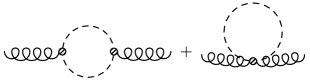
Figure 1.10: Contributions to the self-energy of the $\rho$-meson in standard hadronic models, pion loop (left) and pion tadpole (right). The dashed lines denote pions, the curly ones $\rho$-mesons.

The comparison of the standard hadronic calculations with the static limit provides us with a possibility to estimate the importance of dynamical quark effects. For that purpose we will look at the pion loop in the $\rho$-meson self energy $\Sigma^{\mu\nu}$. We adopt here the usual notation for the self-energy, i.e. the $\rho$-propagator is written as

$$(q^{2}-m_{\rho}^{(0)2}-\Sigma)^{-1}T^{\mu\nu}+{\rm longitudinal~{}parts}~{},$$

with $\Sigma=1/3T_{\mu\nu}\Sigma^{\mu\nu}$. Straightforward evaluation of the corresponding diagram gives

$$g_{\mu\nu}\Sigma^{\mu\nu}_{\rho}(q)=4ig_{\rho\pi\pi}^{2}\Big{\{}I_{1}(m_{\pi})-(q^{2}-4m_{\pi}^{2})I(q,m_{\pi})\Big{\}}~{},$$ (1.138)

with a $\rho\pi\pi$-coupling constant $g_{\rho\pi\pi}$. In the above expression we introduced an additional mass argument for the integrals $I_{1}$ and $I(q)$ in order to indicate that they have to be evaluated at the pion mass $m_{\pi}$ and not, as usual, at the constituent quark mass $m$. If we want to compare this with the static limit of an NJL model calculation we have to pay attention on the fact that the polarization function we usually consider contains a factor $g_{\rho qq}^{2}$ as compared with the usual definition of the self-energy,

$$1-2g_{M}\tilde{\Pi}_{M}(q)=1-2g_{M}(\Pi_{M}(q)+\delta\Pi_{M}(q))=-2g_{M}g_{Mqq}^{-2(0)}(q^{2}-m_{M}^{2\,(0)}+g_{Mqq}^{2(0)}\delta\Pi_{M}(q))~{}.$$ (1.139)

From the structure of that expression we conclude that $\Sigma$ is given by

$$\Sigma_{M}=-g_{Mqq}^{2(0)}\delta\Pi_{M}(q)~{}.$$ (1.140)

For the contribution of the pion loop to the $\rho$-meson self-energy in the static limit we find

$$g_{\mu\nu}\Sigma^{\mu\nu}_{\rho}(q)=16ig_{\rho qq}^{2(0)}\Big{\{}I_{1}(m_{\pi})-(q^{2}-4m_{\pi}^{2})I(q,m_{\pi})\Big{\}}~{}.$$ (1.141)

Comparing this result with Eq. (1.138) and replacing the $\rho$-quark coupling constant by the pion-quark coupling constant using Eq. (1.135), we obtain for the effective $\rho\pi\pi$ coupling constant

$$g^{2}_{\rho\pi\pi}=6g^{2(0)}_{\pi qq}=6\frac{m^{2}}{f^{(0)2}_{\pi}}~{}.$$ (1.142)

If we take the commonly used value of about 6 for $g_{\rho\pi\pi}$ in hadronic models we obtain for the constituent quark mass

$$m\approx\sqrt{6}f^{(0)}_{\pi}~{}.$$ (1.143)

We should remark here that there is some uncertainty in the value we have to take for the pion decay constant in RPA, $f_{\pi}^{(0)}$. In the next chapter we will perform a refit such that the corrected quantities, i.e. $f_{\pi}$ determined either in the MLA or in the $1/N_{c}$-expansion scheme, are equal to the empirical value of $f_{\pi}$. As will be seen in section 2.6.1, $f_{\pi}^{(0)}$ is larger but not much larger than the corrected quantities. In any case, since we are only interested in a rough estimate here we will take a value of $f_{\pi}^{(0)}\sim$ 100-150 MeV. According to Eq. (1.143) this leads to a constituent quark mass of about 250-350 MeV. This is obviously in contradiction to our original assumption of very heavy quarks . Thus, if the main contribution to the momentum dependent quark vertices does not arise from momenta much smaller than 250-350 MeV, we would expect that this approximation does not describe the full model very well. This point will be discussed in more detail in the next section.

In hadronic models one is also interested in the coupling of a bare $\rho$-meson to a photon, which is e.g. needed to calculate the pion electromagnetic form factor via vector-meson dominance. In the NJL model the bare $\rho$-meson corresponds to the RPA meson and its coupling to a photon is basically given by the RPA polarization loop in the vector channel,

$$g_{\rho\gamma}^{\mu\nu}(p)=-i\frac{eg_{\rho qq}^{(0)}}{2}\Pi_{\rho}(p)T^{\mu\nu}(p)~{}.$$ (1.144)

If we now perform the same low-momentum approximations as for the polarization functions we find that the vertex is given by

$$g_{\rho\gamma}^{\mu\nu}(p)=i(e/g_{\rho\pi\pi})p^{2}T^{\mu\nu}(p)$$ (1.145)

which exactly corresponds to the $\gamma\rho$ vertex in the vector dominance model of Kroll, Lee and Zumino [59].

Similar to the proceeding for the $\rho$-meson, approximations to the self-energies of the other mesons can be performed. For instance, this approximation to the $1/N_{c}$-corrected NJL model generates an effective one loop approximation to the linear sigma model in the $\pi$-$\sigma$ sector. The resulting effective meson-meson coupling constants depend on the quark mass and $f_{\pi}^{(0)}$ which in turn depend on temperature and density. This dependence is used in Ref. [60] within a linear sigma model calculation for in-medium pion properties to simulate effects of (partial) chiral symmetry restoration at nonzero temperature and density. This undertaking should, of course, be interpreted with great care since all the effects which can be modulated by their dependence on the quark mass are closely related to unphysical quark effects present in the NJL model due to the lack of confinement. We will discuss this question in more detail in Chapters 2 and  3.2.

Another suggestive approximation to the full momentum dependent calculation is to evaluate the vertices for on-shell intermediate mesons instead of performing a low-momentum expansion. This approximation is discussed in Ref. [32]. However, at least for processes dominated by intermediate pions this gives very similar results to those obtained with the low-momentum expansion.

Chapter 2 Numerical results at zero temperature

In this chapter we will discuss our numerical results at zero temperature. We will begin by a brief description of the regularization scheme and then discuss peculiarities related to the solution of the gap equation in the MLA. After that we will study the influence of mesonic fluctuations on quantities in the pion sector, thereby focusing on possible instabilities. Finally we will perform a refit of these quantities within the $1/N_{c}$-expansion scheme and the MLA and apply the model to observables in the $\rho$-meson sector.

2.1 Regularization

Before we begin the explicit calculation, we will have to fix our regularization scheme. As discussed in Sec. 1.4, all quark loops, i.e. the RPA polarization diagrams, the quark triangles and the quark box diagrams must be regularized in the same way in order to preserve chiral symmetry. Besides Lorentz-covariance being a desirable feature for its own, we prefer for computational convenience a regularization scheme for the quark loops which does not destroy Lorentz-covariance. There are several possible covariant schemes, e.g. proper-time regularization, Pauli-Villars regularization, subtracted dispersion relations or an $O(4)$-cutoff. Some of these have the great disadvantage of displaying the wrong analytic behavior of the RPA meson propagators. For instance an investigation of Broniowski et al. [61] shows that the proper-time regularized RPA meson propagators have poles in the complex plane near the imaginary axis. Subtracted dispersion relations lead to poles for space-like momenta and an $O(4)$-cutoff itself induces a non-analytic structure in the corresponding meson propagator. Since, for the calculation of the mesonic fluctuations, we need the RPA meson propagators for arbritrary four-momenta, we would like to choose a regularization scheme which generates RPA propagators with the correct analytic behavior. At first sight, Pauli-Villars-regularization fulfills both requirements, the covariance and the analyticity of the RPA meson propagators. We will therefore use this regularization scheme. Soon we will become aware that Pauli-Villars regularization is not completely free of peculiarities, either. We will, however, be able to circumvent most of the occurring problems by slightly modifying the standard Pauli-Villars scheme.

To be consistent, all divergent terms should be regularized with the same number of regulators, which is determined by the highest occurring degree of divergence, i.e. the quadratic divergence of the integral

$$I_{1}=\int\frac{d^{4}k}{(2\pi)^{4}}\frac{1}{k^{2}-m^{2}+i{\epsilon}},$$ (2.1)

which we encounter, for instance, in the Hartree gap equation (Eq. (1.4)),

$$m_{H}=m_{0}+2ig_{s}4N_{c}N_{f}m_{H}I_{1}(m_{H})~{}.$$ (2.2)

A quadratic divergence requires two regulators, thus we replace

$$\int\frac{d^{4}k}{(2\pi)^{4}}f(k;m)\;\longrightarrow\;\int\frac{d^{4}k}{(2\pi)^{4}}\sum_{j=0}^{2}c_{j}\,f(k;\mu_{j})~{},$$ (2.3)

by

$$\mu_{j}^{2}=m^{2}+j\,\Lambda_{q}^{2}~{};\qquad c_{0}=1,\quad c_{1}=-2,\quad c_{2}=1~{}.$$ (2.4)

Here $\Lambda_{q}$ is a cutoff parameter. Let us illustrate the standard way to apply this prescription within the NJL model with the RPA polarization loop in the $\sigma$-channel, defined in Eq. (1.11). A straightforward evaluation gives

$$\Pi_{\sigma}(p)=2iN_{c}N_{f}\int\frac{d^{4}k}{(2\pi)^{4}}\Big{(}\frac{2}{k^{2}-m^{2}+i{\epsilon}}-\frac{p^{2}-4m^{2}}{(k^{2}-m^{2}+i{\epsilon})((k+p)^{2}-m^{2}+i{\epsilon})}\Big{)}~{}.$$ (2.5)

Figure 2.1: Inverse $\sigma$-propagator in RPA, $D_{\sigma}^{-1}(p^{2})$, multiplied by $-2g_{s}$ as a function of momentum squared, entire polarization loop regularized (solid line) and only $I_{1}$ and $I(p)$ regularized (dashed line). The parameters used are listed in Table 2.1, for a meson cutoff $\Lambda_{M}=0$ MeV.

The most obvious procedure would be to replace the entire integrand in Eq. (2.5) by the sum over the regulators, see Eq. (2.3). This would be more in the spirit of the original Pauli-Villars regularization [62] than the usual strategy [17], where the polarization loop is written in terms of the already defined elementary integrals $I_{1}$ and $I(p)$,

$$\Pi_{\sigma}(p)=2iN_{c}N_{f}(2I_{1}-(p^{2}-4m^{2})I(p))~{}.$$ (2.6)

Here only the integrals $I_{1}$ and $I(p)$ are regularized, the factor $m^{2}$ in front of $I(p)$ is not modified. The advantage of this strategy can be seen most easily from the inverse $\sigma$-propagator which is displayed in Fig. 2.1 for both methods. This calculation has been performed with the Hartree quark mass. The naive application of Eq. (2.3) to the entire polarization loop obviously leads to a zero of the inverse propagator, i.e. a pole in the propagator, for space-like momenta. The same observation can be made for the $a_{1}$-propagator. This is the reason why we will adopt the usual form of Pauli-Villars regularization in the NJL model and regularize only the divergent elementary integrals throughout this investigation.

We should add a comment on a rather general problem which is related to the regularization of the RPA polarization loops. A straight-forward evaluation of the vector and axial vector polarization diagrams gives

$$\Pi_{\rho}(p) = -i{4\over 3}N_{c}N_{f}\ (-2I_{1}+(p^{2}+2m^{2})\ I(p))~{},$$ (2.7)

$$\Pi_{a_{1}}(p) = -i{4\over 3}N_{c}N_{f}\ (-2I_{1}+(p^{2}-4m^{2})\ I(p))~{}.$$ (2.8)

Because of vector current conservation $\Pi_{\rho}$ should vanish for $p^{2}$ = 0. This is only true if

$$m^{2}\,I(0)=I_{1}~{},$$ (2.9)

which is not the case if we regularize $I(p)$ and $I_{1}$ as described above. Alternatively one could perform the replacement Eq. (2.3) for the entire polarization loop. Then the factor $m^{2}$ in Eqs. (2.7) and (2.9) should be replaced by a factor $\mu_{j}^{2}$ inside the sum over regulators and one can easily show that Eq. (2.9) holds (see Eqs. (A.10) and (A.12)). So it seems as if the strategy we rejected above since it generates poles in the RPA $\sigma$- and $a_{1}$-meson propagators for space-like momenta would be favorable to apply here. However, this scheme leads to another severe problem: From the gap equation (Eq. 2.2) we conclude that $iI_{1}$ should be positive. On the other hand the pion decay constant in the chiral limit and in leading order in $1/N_{c}$, i.e. RPA, is given by, see Eq. (1.83)

$$f_{\pi}^{2(0)}=-2iN_{c}N_{f}\ m^{2}\ I(0)~{},$$ (2.10)

which implies that $im^{2}I(0)$ should be negative. Thus, irrespective of the regularization scheme Eq. (2.9) cannot be fulfilled if we want to get reasonable results for $m_{H}$ and $f_{\pi}^{(0)}$ at the same time. Therefore we will retain our choice of the standard form of Pauli-Villars regularization in the NJL-model and replace the term $I_{1}$ in Eq. (2.7) by hand by $m^{2}\ I(0)$. This leads to the following $\rho$-meson propagator

$$D_{\rho}(p)=\frac{-2g_{v}}{1+2ig_{v}\ {4\over 3}N_{c}N_{f}\ (-2m^{2}\ I(0)+(p^{2}+2m^{2})\ I(p))}~{}.$$ (2.11)

A priori it is not clear whether the symmetry properties of our approximation schemes can be preserved if we perform the above subtraction for the vector polarization function. We noted, however, that this is the case if we take care that the relationship between the RPA $\rho$- and $a_{1}$-meson propagators, Eq. (C.11), is not affected. This can only be achieved if the $a_{1}$-meson polarization function is treated analogously to the vector one. We then arrive at the following RPA $a_{1}$-meson propagator

$$D_{a_{1}}(p)=\frac{-2g_{v}}{1+2ig_{v}\ {4\over 3}N_{c}N_{f}\ (-2m^{2}\ I(0)+(p^{2}-4m^{2})\ I(p))}~{}.$$ (2.12)

After having explained the regularization scheme applied to the quark loops, we will come to discuss the remaining meson-loop integration (integration over $d^{4}p$ in Eq. (1.33)). This integration is not automatically rendered finite by regularizing the quark loops due to the non-renormalizability of the model, so that we have to regularize it separately. This regularization is not constrained by chiral symmetry and independent from the quark-loop regularization. For merely practical reasons we choose a three-dimensional cutoff $\Lambda_{M}$ in momentum space. In order to obtain a well-defined result we work in the rest frame of the “improved” meson. The same regularization scheme was already used in Refs. [39, 40, 42].

From an esthetic point of view, it would certainly be desirable to employ a regularization scheme which allows to render both quark loops and meson loops finite without the introduction of an additional parameter (or as in our case, even another regularization scheme). This could be achieved in a NJL-type model with a separable non-local interaction [28, 63]. This non-local interaction generates a form factor at the quark vertices. That this makes all integrals finite can most directly be seen in the version of Ref. [28]. The authors of Ref. [28] use a form factor which depends on the three-momentum of the quarks. It can be chosen in such a way, that the three-momentum of each quark is limited to absolute values below sum cutoff parameter $\Lambda$. Then simple kinematical considerations lead to the conclusion that the absolute value of the three-momentum of the mesons is automatically restricted to lie below $2\Lambda$. The disadvantage of this model is that it is manifestly non-covariant. In Refs. [63] similar models with form factors depending on the four-momentum are considered. These are obviously covariant, but they have the disadvantage of destroying the analytic properties of the RPA meson propagators. Recently mesonic fluctuations have been investigated [64, 41] within the model presented in Ref. [63].

2.2 Evaluation of the various two-loop diagrams

Within this section we will present some details concerning the rather involved numerical evaluation of the two-loop diagrams contributing for instance to the mesonic polarization functions or the modified gap equation in the MLA, Eq. (1.72).

A general two-loop diagram contains a four-dimensional (momentum) space integration for each loop, i.e. altogether eight integrations. Some of these can usually be performed analytically while the remaining ones have to be performed numerically. Of course one is interested in performing as few as possible integrations numerically since computing time rises and computing precision is reduced steeply the more integrations one has. In our case all the quark loop integrals, i.e. those for the RPA meson propagators and the effective meson-meson vertices, can be written in terms of five “elementary” integrals defined in App. D which in turn, with one exception, can be evaluated analytically. Only for the function

$$L(p_{1},p_{2},p_{3})=\int\frac{d^{4}k}{(2\pi)^{4}}\frac{1}{(k^{2}-m^{2}+i{\epsilon})(k_{1}^{2}-m^{2}+i{\epsilon})(k_{2}^{2}-m^{2}+i{\epsilon})(k_{3}^{2}-m^{2}+i{\epsilon})}~{},$$ (2.13)

with $k_{i}=k+p_{i}$, an analytic expression exists exclusively in kinematical regions where at least one of the momenta lies above the corresponding (in our case quark-antiquark) threshold, i.e. $p_{1}^{2},p_{2}^{2},p_{3}^{2},(p_{1}+p_{2})^{2},(p_{1}+p_{3})^{2}$ or $(p_{2}+p_{3})^{2}$ is larger than $4m^{2}$. This function appears in the four-meson vertex $\Gamma_{M_{1},M_{2},M_{3},M_{4}}(p_{1},p_{2},p_{3})$,  Eq. (1.27). Thus, we are at most left with a one-dimensional integration for the quark loops.

Since we work in the rest frame of the mesons the angular part of the meson-loop integration merely contributes a factor of $4\pi$ and therefore only an integration over energy and the absolute value of the three-momentum remains. The former is most difficult to handle because we have to take care of the various singularities and discontinuities arising from poles and thresholds of the RPA meson propagators and the quark loop vertices. Let us consider for instance the pionic part of the energy integrand for $\delta\Pi^{(a)}$ in the scalar channel

$$\frac{3\,i}{8\pi^{3}}\int_{0}^{\Lambda_{M}}d|\vec{p}|\int_{-\infty}^{\infty}dp_{0}\ \vec{p}^{2}\Gamma_{\sigma,\pi,\pi}(q,p-q/2)\,D_{\pi}(p+q/2)\,\Gamma_{\sigma,\pi,\pi}(-q,-p+q/2)\,D_{\pi}(p-q/2)$$

$$\equiv\frac{3}{8\pi^{3}}\int_{0}^{\Lambda_{M}}d|\vec{p}|\int_{-\infty}^{\infty}dp_{0}\ f(p_{0},|\vec{p}|,q)~{},\hskip 170.71652pt$$ (2.14)

where we have included a factor $3$ due to the sum over the isospin indices of the intermediate pions. We have performed a shift of the integration variable $p\rightarrow p+q/2$ as compared with the definition of $\delta\Pi^{(a)}$ in Eq. (1.33) in order to obtain a function $f(p_{0},|\vec{p}|,q)$ which is symmetric in $p_{0}$, enabling us to restrict the energy integration to the interval $[0,\infty[$ by replacing $f(p_{0},|\vec{p}|,q)$ with $2f(p_{0},|\vec{p}|,q)$. This symmetry property becomes obvious if we take into account that the RPA pion propagator $D_{\pi}(p)$ is only a function of $p^{2}$ instead of $p$ and that the $\sigma\pi\pi$-vertex function $\Gamma_{\sigma,\pi,\pi}(q,p)$ only depends on the momentum of the incoming mesons squared, i.e. $q^{2},(p-q/2)^{2}$ and $(p+q/2)^{2}$. The real and imaginary parts of the symmetrized integrand are shown in Fig. 2.2 for $|\vec{p}|=100$ MeV and two values of $q_{0}$, $100$ MeV and 500 MeV. We have used the parameters listed in Table 2.1 for $\Lambda_{M}=0$ MeV. The most pronounced peaks we observe are the pion poles at $p_{0}=|\pm q_{0}/2+\sqrt{m_{\pi}^{2}+\vec{p}^{2}}|$. Note that we have introduced by hand a small but nonzero imaginary part by replacing the quark mass $m$ in the quark loop integrals with $m-i{\epsilon}$, ${\epsilon}\approx 1$ MeV. One consequence of this nonzero imaginary part is the finite width of the pion poles. More or less steep quark-antiquark thresholds appear if one of the momenta, i.e. $q^{2},(p+q/2)^{2}$ or $(p-q/2)^{2}$, equals $4m^{2}$. These are invisible in Fig. 2.2 because of the much larger scale of the singularities arising from the pion poles. Additional thresholds exist due to the Pauli-Villars regulator masses $m^{2}+\Lambda_{q}^{2}$ and $m^{2}+2\Lambda_{q}^{2}$, see Eq. (2.4).

Figure 2.2: Integrand for the $p_{0}$-integration, pionic part of the contribution $\delta\Pi^{(a)}$ to the $\sigma$-meson polarization function with $|\vec{p}|=100$ MeV, real (solid) and imaginary part (dashed), for $q_{0}=100$ MeV (left) and $q_{0}=500$ MeV (right).

The values of $q_{0}=100$ MeV and $q_{0}=500$ MeV have been chosen for the following reason: The former value for $q_{0}$ lies below any threshold and we expect no imaginary part to be present at the end, the latter above the two-pion threshold at $280$ MeV. The results we obtain for the imaginary part below any thresholds are very sensitive to the details of the numerical evaluation. Calculating this imaginary part, which we know to vanish, serves as a sensitive measure for the precision of our delicate numerical integration procedure. An imaginary part is always related to a decay process, e.g. $\sigma\rightarrow\pi\pi$. The three-dimensional cutoff we apply for the $|\vec{p}|$-integration can at most restrict the phase space for that decay. If for example $q_{0}>2\sqrt{m_{\pi}^{2}+\Lambda_{M}^{2}}$, then no decay is possible, thus the cutoff can suppress a decay process but in no way generate one, and consequently no imaginary part. From this we conclude that the energy integration alone has to be responsible for the imaginary part vanishing below any threshold. Thus the integration over the imaginary part of $f(p_{0},|\vec{p}|,q)$ has to vanish for $q_{0}<280$ MeV, e.g. for $q_{0}=100$ MeV. Looking at Fig. 2.2 one realizes that this is a completely non-trivial undertaking. Particular attention should be paid to three crucial points: to proper integration over singularities and thresholds, to an extrapolation to vanishing ${\epsilon}$, and to the inclusion of high-energy contributions. The first and the second point are connected, since the quantity ${\epsilon}$ has been introduced by hand to soften the otherwise numerically not tractable singularities and thresholds. This artificial width enables us, by suitably adapting the location and number of mesh points in the vicinity of singularities and thresholds, to perform the integration with sufficient precision. The limit ${\epsilon}\rightarrow 0$ is approximated thereafter by linear extrapolation. Including also contributions from very high energies turns out to be difficult because the evaluation of the integrand becomes numerically unstable for very large energies, i.e. $p_{0}\mathrel{\raise 1.29167pt\hbox{$>$\kern-7.5pt\lower 4.30554pt\hbox{$\sim$}}}$ 15 GeV. However, at least for the imaginary part these contributions cannot be neglected since they are necessary for cancellations below any threshold. An integration up to $p_{0}\rightarrow\infty$ can be achieved by first applying one of the standard substitutions of the integration variable: For large energies, i.e. above any threshold, we substitute $p_{0}=\tan(x)$. The resulting function of $x$ can very well be approximated by a quadratic function and thus can easily be extrapolated up to the upper integration boundary of $\pi/2$. The real part remains almost unaltered by the operations described above.

Figure 2.3: Integrand for the $|\vec{p}|$-integration, pionic part of the contribution $\delta\Pi^{(a)}$ to the $\sigma$-meson polarization function, real (solid) and imaginary part (dashed), with (left) $q_{0}=100$ MeV and (right) $q_{0}=500$ MeV.

The finally rather satisfying result can be seen in Fig. 2.3 where we have plotted the corresponding integrand for the $|\vec{p}|$-integration. The left panel represents the result for $q_{0}=100$ MeV, the right panel that for $q_{0}=500$ MeV. For $q_{0}=100$ MeV the imaginary part is suppressed by 5 orders of magnitude as compared with the real part which reveals the efficiency of our method of integration. The $|\vec{p}|$-integration is comparatively easy to handle. For $q_{0}=100$ MeV the integrand is completely smooth, for $q_{0}=500$ MeV only in the vicinity of $|\vec{p}|=\sqrt{q_{0}^{2}/4-m_{\pi}^{2}}$, i.e. $|\vec{p}|=207$ MeV, we have to be a little careful with placing the mesh points for the integration. In most other cases, more precisely in all cases where we do not have to deal with a two-pion intermediate state, we also end up with a completely smooth function for the $|\vec{p}|$-integration.

2.3 Solution of the gap equation in the MLA

In the $1/N_{c}$-expansion scheme all diagrams are calculated with the constituent quark mass in Hartree approximation, i.e. as it emerges from the Hartree gap equation, Eq. (1.2). In the MLA, on the contrary, the quark mass is determined by the solution of the extended gap equation, Eq. (1.72), which was derived in section 1.3.3 from a one-meson-loop approximation to the effective action. The structure of this extended gap equation was indispensable in order to prove the validity of various symmetry relations, namely the Goldstone theorem, the Goldberger Treiman relation and the GOR relation, in section 1.4.2. This is not astonishing since the entire scheme is based on the extended gap equation. However, only the structure of this equation has been used but not the explicit solution. This section is now devoted to a discussion of the explicit solution of the extended gap equation. Unforeseen problems occur which will force us to slightly modify the scheme.

First indications for these problems can already be inferred from the behavior of the RPA mesons as a function of a trial constituent mass $m$. As already pointed out, the RPA mesons, which enter the extended gap equation (see Fig. 1.9), have to be evaluated with the selfconsistently determined quark mass $m^{\prime}$, which is in general different from the Hartree quark mass $m_{H}$. Hence, the propagators of these mesons differ from those in the Hartree + RPA scheme. To illustrate this let us look at the masses of the pion and $\sigma$-meson in the RPA as a function of a trial quark mass $m$ displayed on the l.h.s. of Fig. 2.4. We have used the parameters listed in Table 2.1 with $\Lambda_{M}=0$ MeV. The effects of $\pi$-$a_{1}$-mixing can be governed by manipulating the vector coupling constant $g_{v}$: With a vanishing $g_{v}$, $\pi$-$a_{1}$-mixing is turned off, with an increasing $g_{v}$ it becomes more and more important. For comparison we have computed the pion mass with $g_{v}=0$ (solid line) and $g_{v}=2g_{s}$ (dotted line). The mass of the $\sigma$-meson (dashed line) does not depend on $g_{v}$. The principal observation is that the pion becomes tachyonic, i.e. $m_{\pi}^{(0)2}$ becomes negative, for quark masses smaller than the Hartree quark mass. Strictly speaking this is only true in the chiral limit, for nonvanishing current quark masses we find negative $m_{\pi}^{(0)2}$ at first for quark masses slightly below $m_{H}$.

Qualitatively the results do not change if $\pi$-$a_{1}$-mixing is included. If we keep all parameters fixed, it can be seen from the explicit form of the pion propagator in the RPA (Eqs. (C.4) and (B.5)), that in the chiral limit the results even do not change at all. Away from the chiral limit the pion mass is slightly increased and hence the trial quark mass, where the pion mass vanishes, is slightly decreased. In principle, the parameters should be refitted with the pion mass fixed to its empirical value at $m=m_{H}$, which diminishes the influence of $\pi$-$a_{1}$-mixing on the value of the quark mass $m$ where the pion becomes tachyonic.

A similar observation can be made for $m_{\sigma}^{(0)2}$, but only for $m$ much smaller than the Hartree mass. This finding of tachyonic RPA mesons for certain quark masses causes the meson-loop term in the effective action (second term in Eq. (1.55)) to be no longer positive definite in that range of quark masses. As discussed in section 1.3.3 this reveals that the effective action is ill-defined in that range.

Figure 2.4: (Left) Squared pole masses of the pion with $g_{v}=0$ (solid), $g_{v}=2g_{s}$ (dotted) and the $\sigma$-meson (dashed) in RPA as functions of a trial constituent quark mass $m$ in units of the Hartree quark mass. (Right) Difference $m-m_{0}-\tilde{\Sigma}(m)$ between the l.h.s. and the r.h.s. of the MLA gap equation, Eq. (1.72), as a function of the trial constituent quark mass $m$. The real part is denoted by the solid line for $g_{v}=0$ and by the dashed-dotted line for $g_{v}=2g_{s}$, the imaginary part by the dashed line for $g_{v}=0$ and by the dotted line for $g_{v}=2g_{s}$.

The latter point becomes obvious if we look at the quark self-energy which becomes complex if it is calculated with tachyonic RPA mesons. Therefore we have to hope that a solution of the extended gap equation can be found which is larger than the Hartree mass. Any other solution necessarily must be complex or negative. To illustrate this point we consider the difference between the l.h.s. and the r.h.s. of the extended gap equation, Eq. (1.72), as function of a (real) trial mass $m$. This difference is plotted in the right panel of Fig. 2.4. Let us begin the discussion by the results obtained with $g_{v}=0$, i.e. we turn off effects of $\pi$-$a_{1}$-mixing and the contributions of vector and axial intermediate states in $\delta\tilde{\Sigma}$. The solid line denotes the real part for this case, the dashed line the imaginary part of $m-m_{0}-\tilde{\Sigma}(m)$. Evidently the self-energy indeed becomes complex for quark masses below some mass $m_{c}$. A comparison with the pion mass reveals that $m_{c}$ coincides with the quark mass below which the pion becomes tachyonic. A kink in the real as well as in the imaginary part indicates the point where also the sigma becomes tachyonic. Moreover, we see that there is no solution of the gap equation for real constituent quark masses besides the trivial solution at $m=0$. Hence, solutions, if there exists any, lie somewhere in the complex plane off the positive real axis. Consequently the RPA mesons would be built of quarks with either complex or negative masses leading to peculiar properties. In any case this renders a reasonable description of the mesons in MLA completely impossible. This is most clearly seen for the $\rho$-meson, whose properties are mainly determined by intermediate RPA pions. Including vector and axial vector intermediate states as well as $\pi$-$a_{1}$-mixing does not alter this troubling result, since, qualitatively, the function $m-m_{0}-\tilde{\Sigma}(m)$ shows the same behavior in the case of $g_{v}=2g_{s}$. It is displayed on the r.h.s. of Fig. 2.4, the dashed-dotted line corresponds to the real part, the dotted line to the imaginary part.

A possible way out of this dilemma is to perform a modification, which has been introduced in Ref. [30]. Of course, any approximation we perform has to preserve the symmetry properties of the MLA. As discussed in section 1.4.2 this can be achieved if the validity of Eq. (1.91) for the RPA meson propagators is not affected. This remains true if we include vector and axial vector intermediate states, see App. C.2. In that case in addition to Eq. (1.91) for the pion and $\sigma$-meson propagators a similar relationship for the RPA $\rho$- and $a_{1}$-meson propagators has to hold. Thus the approximation suggested in Ref. [30] for the purely scalar and pseudoscalar case can straightforwardly be generalized to the case with vector and axial vector interaction. This will be shown in more detail in App. C.2, here we will only illustrate the principle of this approximation which can be done most easily if we set $g_{v}=0$.

The authors of Ref. [30] simply replace the RPA pion propagator in the extended gap equation,

$$D_{\pi}(p)=-2g_{s}\;\Big{[}\;1\;-\;2ig_{s}\;4N_{c}N_{f}\int\frac{d^{4}k}{(2\pi)^{4}}\frac{1}{k^{2}-m^{2}+i\varepsilon}+2ig_{s}(2N_{c}N_{f})\,p^{2}\,I(p)\,\Big{]}^{-1}$$ (2.15)

by

$$D_{\pi}(p)=-2g_{s}\;\Big{[}\,\frac{m_{0}}{m}+2ig_{s}\;2N_{c}N_{f}\,p^{2}\,I(p)\,\Big{]}^{-1}$$ (2.16)

and analogously for the $\sigma$-propagator. It is clear from the proof of the Goldstone theorem in section 1.4.2 that the same replacements have to be performed for the RPA meson propagators in the correction terms $\delta\Pi_{M}^{(k)}$ to the mesonic polarization diagrams. In addition chiral symmetry requires that the RPA contribution to the mesonic polarization function, $\Pi_{M}$, itself is not changed. By performing this approximation we not only obtain a real (positive) solution of the extended gap equation but also the masses of the intermediate mesons remain real. Moreover, we obtain massless intermediate pions in the chiral limit, which becomes obvious by looking at Eq. (2.16). Besides, the various symmetry relations proved in section 1.4.2 still hold.

We can certainly ask whether there is any other motivation for this approximation in addition to the practical reasons discussed above. In the Hartree approximation, i.e. if the RPA mesons are calculated with quarks of mass $m_{H}$, the above replacements would be exact. Following the arguments put forward by the authors of Ref. [30], the correction terms we neglect by performing the above replacements would be suppressed, because they are of higher order in $1/N_{c}$. This is of course a questionable argument in the MLA since already the quark mass $m^{\prime}$, the selfconsistent solution of the extended gap equation, contains arbitrary orders in $1/N_{c}$. In fact, we have seen that this approximation drastically changes the results.

We will keep the name “one-meson-loop approximation” for this scheme, including the above replacements, although this is strictly speaking only an approximation to the MLA as it was originally introduced in section 1.3.3.

2.4 Meson-loop effects on quantities in the pion sector

The additional cutoff $\Lambda_{M}$ we introduced in section 2.1, enables us to study the influence of mesonic fluctuations on several quantities, e.g. the quark condensate or the pion mass $m_{\pi}$ and the pion decay constant $f_{\pi}$. This cutoff restricts the momentum of the intermediate meson states. We can therefore, by slowly turning on this cutoff, control the importance of the mesonic fluctuations. For $\Lambda_{M}=0$ we of course recover the usual RPA result. It is advantageous to keep all other parameters constant. We use $m_{0}=6.13$ MeV, $\Lambda_{q}=800$MeV and $g_{s}\Lambda_{q}^{2}=2.90$. These parameter values are chosen in such a way that $m_{\pi}^{(0)},f_{\pi}^{(0)}$, and $\langle{\bar{\psi}\psi}\rangle^{(0)}$ reproduce the empirical values. We obtain, for $g_{v}=0$, $m_{\pi}^{(0)}=140.0$ MeV, $f_{\pi}^{(0)}=93.6$ MeV and $\langle{\bar{\psi}\psi}\rangle^{(0)}=-2(241.1~{}{\rm MeV})^{3}$. For the constituent quark mass in the Hartree approximation we get $m_{H}=260$ MeV. These values are slightly changed if we include vector mesons, i.e. $g_{v}\neq 0$. In the following section we will discuss our results for the quark condensate, in section 2.4.3 we will consider the properties of the pion, among other things $m_{\pi}$ and $f_{\pi}$ which are related to the quark condensate via the GOR relation.

Of course, an application of the approximation schemes, the $1/N_{c}$-expansion scheme and the MLA, to physical processes will only be meaningful if a refit of the parameters is performed to reproduce the empirical values of $m_{\pi},f_{\pi}$ and $\langle{\bar{\psi}\psi}\rangle$. This will be discussed in section 2.6.1.

2.4.1 Quark condensate

The behavior of the quark condensate as a function of the mesonic cutoff $\Lambda_{M}$ is displayed in Fig. 2.5. The upper panel shows the results in the chiral limit and the lower panel those with $m_{0}=6.13$ MeV, i.e. with a realistic pion mass. The solid lines correspond to $g_{v}=0$, i.e. excluding vector interactions, and the dashed lines to $g_{v}=2g_{s}$. We will begin the discussion by the results obtained without vector and axial vector intermediate states which were already investigated in Ref. [42]. We observe that in the chiral limit as well as with a nonvanishing current quark mass the absolute value of the quark condensate decreases first with an increasing cutoff and then, if the cutoff exceeds a certain value, goes up again. This feature is common to the $1/N_{c}$-expansion scheme (left panel) and the MLA (right panel). This effect is related to an unphysical pole in the pion propagator we detect for large values of the cutoff, see section 2.5. Studying the effects of vector and axial vector fluctuations is an interesting issue in the context of a suggestion made by Plant and Birse [41], saying that these instabilities do not survive if one takes into account fluctuations of vector and axial vector mesons and especially the $\pi$-$a_{1}$-mixing. They corroborate this suggestion by a calculation of the quark self-energy in a generalized, non-local, version of the NJL model (cf. section 2.1). Without vector meson intermediate states they encounter in next-to-leading order in $1/N_{c}$ a minimum in the self-energy for large momenta, whereas the vector and axial vector states seem to suppress this effect.

Figure 2.5: The ratio $\langle{\bar{\psi}\psi}\rangle/\langle{\bar{\psi}\psi}\rangle^{(0)}$ as a function of the meson cutoff $\Lambda_{M}$. The solid line corresponds to $g_{v}=0$, i.e. the result without vector and axial intermediate states, the dashed line to $g_{v}=2g_{s}$, (left) $1/N_{c}$-expansion scheme, (right) MLA. The curves in the upper panel are calculated with a vanishing current quark mass, in the lower panel the corresponding results with a realistic value of $m_{0}=6.13$ MeV are shown.

Considering the results with $g_{v}=2g_{s}$ we should primarily state that the influence of the vector and axial vector fluctuations is remarkably big. In the $1/N_{c}$-expansion scheme the minimum does not vanish, neither in the chiral limit nor with a nonzero current quark mass. It is only relocated at higher values of the cutoff. It becomes even more steep compared with the case without vector and axial mesons. In the MLA the minimum has entirely disappeared. Looking at the results in the chiral limit we instead observe a behavior typically for a phase transition: For small values of the cutoff the quark condensate rapidly approaches zero, at $\Lambda_{M}\mathrel{\raise 1.29167pt\hbox{$>$\kern-7.5pt\lower 4.30554pt\hbox{$\sim$}}}$450 MeV it vanishes. The slope of the condensate at the “critical cutoff” diverges, indicating indeed a phase transition of second or first order. In section 2.5 we will establish a conclusive answer to the nature of this phase transition from the effective potential. In that section we will also explain how the calculations in the chiral limit, numerically a difficult task, are actually performed. For $m_{0}=6.13$ MeV the condensate shows the typical cross-over behavior: For small values of $\Lambda_{M}$ it rapidly approaches zero, at $\Lambda_{M}\approx 550$ MeV the slope rather abruptly changes such that the quark condensate seems to reach zero asymptotically.

The authors of Ref. [41] state that mainly the longitudinal parts of the vector mesons are responsible for the disappearing of the minimum. In our case, as shown in section 1.5, the $\rho\rho\sigma$-vertex is transverse and hence the longitudinal part of the $\rho$-meson gives no contribution at all, whereas the longitudinal part of the axial polarization, absorbed in the pion propagator via $\pi$-$a_{1}$-mixing, can very well be important.

To investigate this question we will look at the constant $\Delta$ which is the main element of the corrections to the quark condensate, both in the $1/N_{c}$-expansion scheme and in the MLA. In the $1/N_{c}$-expansion scheme this can be seen directly (cf. Eqs. (1.6) and (1.32)): As a function of $\Lambda_{M}$ the Hartree contribution and the RPA $\sigma$-propagator remain constant. Thus the mesonic fluctuations can only have an effect on $\Delta$. In the MLA this connection is not as obvious since we have to solve Eq. (1.72) selfconsistently. Nevertheless the qualitative behavior of the quark condensate can be deduced from that of $\Delta$. In order to understand the peculiar “turn-around” as a function of the meson cutoff $\Lambda_{M}$, it is convenient to look at the integrand instead of $\Delta$ itself. The function $F(|\vec{p}|)$, displayed in Fig. 2.6, has to be integrated over $|\vec{p}|$ to obtain $\Delta$. This representation allows us to estimate the influence of the cutoff value on the result for $\Delta$. We show the contributions of the different mesonic intermediate states and the corresponding sum, on the left hand side we neglected the $\rho$- and $a_{1}$-meson subspace, whereas on the right hand side it is included (together with $\pi$-$a_{1}$-mixing).

Let us begin our discussion by the purely scalar-pseudoscalar case. The sum of both contributions first rises, then, at $|\vec{p}|\sim 445$ MeV, it starts to decrease. At $|\vec{p}|\sim 900$ MeV it even crosses the axis and its slope indicates that it will become more and more negative for larger values of $|\vec{p}|$. We see that the pionic contribution is much more important than the contribution from $\sigma$-meson intermediate states. It also mainly produces the negative contributions which are responsible for the “turn-around” of the quark condensate as a function of the cutoff. The contribution of the $\sigma$-meson of course remains completely unchanged if we include vector and axial intermediate states. The pionic one, however, is affected by $\pi$-$a_{1}$-mixing. As can be seen on the r.h.s. of Fig. 2.6 the decrease of the pionic contribution is weakened and shifted to higher momenta. The (transverse) vector contribution is mainly responsible for the decrease of the integrand, whereas the tranverse part of the axial one, i.e. the $a_{1}$, tends to increase it. The maximum and the zero of the overall sum is relocated at higher absolute values of the three-momentum compared with the purely scalar-pseudoscalar case, but qualitatively the behavior is not altered. This observation is directly reflected in the behavior of the quark condensate in the $1/N_{c}$-expansion scheme, where vector interactions only lead to a shift of the observed minimum as a function of the mesonic cutoff $\Lambda_{M}$ to higher energies. In the MLA, however, the relation between $\Delta$ and the quark condensate is less direct mainly because of the selfconsistent determination of quark condensate. In any case also in the MLA the general behavior remains unaltered.

Figure 2.6: Integrands for $\Delta$ as a function of $|\vec{p}|$. (Left:) $g_{v}=0$, contribution from the pion (dashed line), $\sigma$-meson (dotted), and the sum of both contributions (solid). (Right:) $g_{v}=2g_{s}$, contribution from the pion (dashed), $\sigma$-meson (dotted), $\rho$-meson (short-dashed), $a_{1}$-meson (dashed-dotted), and the sum of all contributions (solid).

2.4.2 Problems with vector intermediate states

Before we begin our discussion of pionic properties let us explain the difficulties we encounter if we try to include vector and axial vector meson intermediate states for the calculation of the corrections to the mesonic polarization functions. The problem is related to the rather general problem discussed in section 2.1 of preserving the consequences of current conservation for the vector propagator in RPA, i.e. transversality and $\Pi_{\rho}(0)=0$, and simultaneously not inducing wrong analytical properties for $\sigma$- and $a_{1}$-mesons. As an example we will consider the diagram $(b)$ in Fig. 1.4. It contains among other contributions one four-meson vertex where two external pions with momentum $q$ couple to an axial state with momentum $p$. Contracting this vertex with $p_{\mu}p_{\nu}/p^{2}$ we receive contributions to the integral for $\delta\Pi_{\pi}^{(b)}(q)$, defined in Eq. (1.33), from an $a_{1}$-meson as well as from the axial part of the pion. In fact, the resulting scalar vertex function,

$$-i\frac{p_{\mu}p_{\nu}}{p^{2}}\delta_{bc}\Gamma_{\pi,a_{1},a_{1},\pi}^{{\mu\nu},abcd}(q,p,-q) =$$ (2.17)

$$-12N_{c}N_{f}\Big{(}\phantom{+}I(p+q)(p+q)^{2}-I(q)(q^{2}+p\cdot q)-I(0)p\cdot q$$

$$\phantom{-12N_{c}N_{f}\Big{(}}+K(q)q^{2}(p\cdot q-p^{2})+4m^{2}p^{2}K(p)-4m^{2}\,p^{2}\,q^{2}L(p,-q,0)\Big{)}$$

is multiplied by the difference of the RPA $a_{1}$-meson propagator and the axial part of the pion propagator, $D_{a_{1}}(p)-D_{\pi_{v}}(p)$.

The problem arises from the combination of two types of terms: The first type are addends proportional to $1/p^{2}$, e.g. the term $q^{2}/p^{2}I(q)$ in Eq. (2.17), the second type are terms depending only on the momentum $q$, i.e. being constant with respect to the integration variable $p$, e.g. the term $q^{2}K(q)$ in Eq. (2.17). Thus, on the one hand the difference of the RPA $a_{1}$-propagator and the axial part of the pion propagator should vanish as $p^{2}$ for $p^{2}\rightarrow 0$ in order not to produce unphysical poles at $p^{2}=0$, and on the other hand it should vanish at least as $1/p_{0}$ for large energies to guarantee the convergence of the energy integration. Using the explicit expressions for the $a_{1}$-propagator and the axial part of the pion propagator given in Eqs. (2.12) and (C.4), respectively, we see that the difference vanishes at $p^{2}=0$. Hence we can conclude that the first condition is fulfilled for the RPA propagators in their present form. Since the three-dimensional cutoff $\Lambda_{M}$ restricts the absolute value of the three-momentum $|\vec{p}|$, we can gain insight into the behavior of the difference for large energies by looking at it for large $p^{2}$. Using the properties of the Pauli-Villars regulators introduced in Eq. (2.3) we infer that the integral $I(p)$ in leading order behaves like

$$I(p)\rightarrow 2\frac{I_{1}}{p^{2}}~{};\quad{\rm for}\quad p^{2}\gg m^{2}~{}.$$ (2.18)

This enables us to conclude that the difference of the RPA $a_{1}$-propagator and the axial part of the pion propagator contains besides terms vanishing at least with $1/p^{2}$ a constant term proportional to

$$-m^{2}I(0)+I_{1}~{}.$$

This term is reminiscent of the $a_{1}$ polarization function. Note that the subtraction we performed in section 2.1 in order to preserve gauge invariance for the vector polarization function here induces this problem. On the other hand a closer examination shows that the difference would not vanish at $p^{2}=0$ if we had not performed this subtraction. Thus the only solution seems to be providing for Eq. (2.9) to hold. This is a dilemma since we saw in section 2.1 that this leads to even more severe problems. We therefore decided to put the vector and axial vector meson intermediate states aside and will only treat scalar and pseudoscalar states throughout the remaining part of this paper.

2.4.3 Pion Properties

In this subsection we want to study the influence of mesonic fluctuations on the pion propagator, which will enable us to study especially the effects on the pion mass and the pion decay constant, both within the $1/N_{c}$-expansion scheme and within the MLA. Major parts of this analysis can be found in Refs. [39, 42]. We proceed in the same way as in the previous subsection: Since the strength of the fluctuations is controlled by the meson cutoff $\Lambda_{M}$, we first keep all other parameters fixed and investigate how the above quantities change, when $\Lambda_{M}$ is varied.

Figure 2.7: Squared pion mass as a function of the current quark mass $m_{0}$ for different meson-loop cutoffs; (left) $1/N_{c}$-expansion scheme: $\Lambda_{M}$ = 0 MeV (solid), 500 MeV (dashed), 900 MeV (dashed-dotted) and 1300 MeV (dotted); (right) MLA: $\Lambda_{M}=0$ MeV (solid), 300 MeV (dashed), 500 MeV (dashed-dotted) and 700 MeV (dotted). The calculated points are explicitly marked.

Fortunately, the pion mass provides us with a decisive test for the stability of the rather involved numerics. The Goldstone theorem, which was proved analytically in section 1.4 for the $1/N_{c}$-expansion scheme and the MLA, clearly states that the pion mass has to vanish for a vanishing current quark mass $m_{0}$. For numerical reasons we cannot compute the pion mass exactly in the chiral limit, but its value can be extrapolated from the behavior of the squared pion mass as a function of the current quark mass $m_{0}$. This is displayed in Fig. 2.7 for different values of $\Lambda_{M}$, on the l.h.s. evaluated within the $1/N_{c}$-expansion scheme, on the r.h.s. in the MLA. Obviously the dependence in both schemes is almost linear, i.e. the analytically calculated point at $m_{0}=0,m_{\pi}^{2}=0$ and the numerically computed points, corresponding to the same cutoff, lie almost on a straight line. This result is suited for convincing us of the consistency of our calculations with chiral symmetry and of the stability of the numerics.

Now we fix the current quark mass again to $m_{0}=6.13$ MeV and slowly turn on the mesonic cutoff $\Lambda_{M}$ and with it the strength of the mesonic fluctuations. The resulting behavior of $m_{\pi}^{2}$ and $f_{\pi}^{2}$ as a function of $\Lambda_{M}$ is displayed in Fig. 2.8. The left panel shows the results for the $1/N_{c}$-expansion scheme, the right panel for the MLA. It is clearly visible, that the qualitative behavior of $f_{\pi}$ and $m_{\pi}$ turns out to be the same in both schemes: The first (dashed lines) is reduced whereas the latter (solid) is increased. If only $\sigma$ and $\pi$ intermediate states are considered it was observed in the previous section that both schemes show similar results for the quark condensate.

Figure 2.8: The ratios $m_{\pi}^{2}/{m_{\pi}^{2}}^{(0)}$ (solid), $f_{\pi}^{2}/{f_{\pi}^{2}}^{(0)}$ (dashed), and the combination $-m_{0}\langle{\bar{\psi}\psi}\rangle/m_{\pi}^{2}f_{\pi}^{2}$ (dotted) as a function of the meson loop cutoff $\Lambda_{M}$ in the $1/N_{c}$-expansion scheme (left) and the MLA (right).

In section 1.4.1 we showed that in the Hartree approximation + RPA the quantities ${m_{\pi}^{2}}^{(0)}$, ${f_{\pi}^{2}}^{(0)}$ and $\langle{\bar{\psi}\psi}\rangle^{(0)}$, should be in good agreement with the GOR relation, Eq. (1.80). This should also hold for the corresponding quantities $m_{\pi},f_{\pi}$, and $\langle{\bar{\psi}\psi}\rangle$ in the MLA, see section 1.4.2. The $1/N_{c}$-expansion scheme, on the contrary, is consistent with the GOR relation only up to next-to-leading order and, as discussed in section 1.4.3, the “corrected” quantities violate the relation by higher-order terms. For this reason we expect a less perfect agreement in this scheme, becoming worse with increasing values of $\Lambda_{M}$.

These expectations are more or less confirmed by the results. In the Hartree + RPA scheme we find only deviations -due to corrections in higher orders in $m_{0}$- of about 0.1%. In the MLA the deviations are slightly larger, due to the numerics being much more difficult to handle. One reaches up to about 3% for a cutoff of $\Lambda_{M}=900$ MeV. These deviations can be inferred from the ratio of the r.h.s. and the l.h.s. of the GOR relation, Eq. (1.80), displayed in Fig. 2.8 by the dotted lines. As can be seen, in the MLA (right panel) it almost coincides with the desired value of $1$, whereas in the $1/N_{c}$-expansion scheme (left panel) we indeed observe considerable discrepancies. Within this scheme the GOR relation holds at least within 30% for $\Lambda_{M}\leq$ 900 MeV, tolerable for higher-order corrections in this perturbative scheme. However, when the meson cutoff is further increased the agreement with the GOR relation rapidly deteriorates, indicating that in this regime higher-order corrections become important. Our perturbative scheme should not be trusted there any more.

One may wonder why we do not plot the various curves for cutoffs larger than $\Lambda_{M}=1250$ MeV in the $1/N_{c}$-expansion scheme and $\Lambda_{M}=900$ MeV in the MLA. The reason is that upon further increasing $\Lambda_{M}$ we detect a second, unphysical, pole in the pion propagator [39, 42]. This phenomenon will be discussed in more detail in the next section.

2.5 Instabilities due to strong mesonic fluctuations?

As already mentioned it has recently been claimed by Kleinert and van den Bossche [43] that in the NJL model chiral symmetry, which is spontaneously broken in the mean field ground state, gets restored due to strong mesonic fluctuations. One principal objection one can raise against this supposition is the non-renormalizability of the NJL model. Including fluctuations beyond mean-field we cannot avoid encountering additional divergencies. Thus a priori an additional cutoff parameter has to be introduced as discussed previously. This additional cutoff parameter then controls the strength of mesonic fluctuations [39]. Nevertheless it might be possible to observe some kind of “chiral symmetry restoration” at a certain value of the cutoff parameter.

Figure 2.9: Inverse pion propagator, $D_{\pi}^{-1}$, multiplied by $-2g_{s}$ as a function of the 4-momentum squared for various meson cutoffs; in the $1/N_{c}$-expansion scheme (left): $\Lambda_{M}$ = 0 (solid), 900 MeV (dashed), 1300 MeV (dashed-dotted) and 1500 MeV (dotted) and the MLA (right): $\Lambda_{M}=0$ MeV (solid), 500 MeV (dashed), 700 MeV(dashed-dotted) and 1100 MeV (dotted).

In the previous section we stated that a second, unphysical, pole emerges in the pion propagator if the cutoff exceeds a certain value. This pole has a residue of the “wrong” sign, leading to an imaginary pion-quark coupling constant and a negative value for the squared pion decay constant $f_{\pi}^{2}$. This becomes clear from Fig. 2.9, where the inverse pion propagator $D_{\pi}^{-1}$ is plotted as a function of the momentum squared $q^{2}$ for different values of the cutoff $\Lambda_{M}$. The left panel shows the results in the $1/N_{c}$-expansion scheme, the right panel those in MLA. In the chiral limit all curves would go through $-2g_{s}D_{\pi}^{-1}=0$ at $q^{2}=0$ with a negative slope. In the Hartree approximation + RPA the effect of a non-zero current quark mass is to shift this value up to $m_{0}/m_{H}$, i.e. the zero of the inverse propagator, corresponding to the pole of the propagator, is then located at some positive (time-like) value of $q^{2}$. In the $1/N_{c}$-expansion scheme the main effect of the meson-loop contributions for $\Lambda_{M}\mathrel{\raise 1.29167pt\hbox{$<$\kern-7.5pt\lower 4.30554pt\hbox{$\sim$}}}900$ MeV is to further increase the value of $D_{\pi}^{-1}$ at $q^{2}=0$ and with it the value of $q^{2}$ at the zero, i.e. the pion mass. Upon further increasing $\Lambda_{M}$ the value of $D_{\pi}^{-1}(0)$ is again reduced. From Eqs. (1.95) and (1.110) we conclude that the $1/N_{c}$-correction terms to $D_{\pi}^{-1}(0)$ are proportional to $\Delta$. Thus, the behavior of $D_{\pi}^{-1}(0)$ reflects that of the constant $\Delta$, discussed in section 2.4.1. At the same time the curve flattens considerably, leading to a strongly rising pion mass. For $\Lambda_{M}\mathrel{\raise 1.29167pt\hbox{$>$\kern-7.5pt\lower 4.30554pt\hbox{$\sim$}}}1250$ MeV we observe that it turns around below the quark-antiquark threshold, causing the second pole in the pion propagator. Obviously the slope of $D_{\pi}^{-1}$ at this second zero is inverse as compared with the first zero. This reveals the above mentioned fact of a residue with the “wrong” sign. When the cutoff is further increased the two zeros move towards each other, merging at $\Lambda_{M}\approx 1350$ MeV and disappearing thereafter from the real positive $q^{2}$-axis. Qualitatively the same behavior is observed within the MLA. The only difference is that the second unphysical zero emerges already for $\Lambda_{M}\mathrel{\raise 1.29167pt\hbox{$>$\kern-7.5pt\lower 4.30554pt\hbox{$\sim$}}}910$ MeV and the two poles merge already for $\Lambda_{M}\approx 1095$ MeV.

Figure 2.10: Real (upper panel) and imaginary part (middle) of the different $1/N_{c}$-correction terms to the pion polarization function, $\delta\Pi_{\pi}^{(a)}$ (long-dashed), $\delta\Pi_{\pi}^{(b)}$ (dotted), $\delta\Pi_{\pi}^{(c)}$ (short-dashed), and $\delta\Pi_{\pi}^{(d)}$ (dashed-dotted), for $\Lambda_{M}=700$ MeV (left), and 1100 MeV (right). Different corrections term to the pion polarization function in the MLA for $\Lambda_{M}=1000$ MeV (lower panel), $\delta\Pi^{(a)}$ (long-dashed), $\delta\Pi^{(b)}$ (dotted), and $\delta\Pi^{(c)}$ (short-dashed), real part (left) and imaginary part (right).

Within both schemes this unphysical behavior can be traced back mainly to the contributions from $\delta\Pi_{\pi}^{(b)}$. This term has a peak in the imaginary part above the $\bar{q}q$-threshold with the “wrong” sign. This can be seen from Fig. 2.10, where the various contributions to the pion polarization function are displayed. For low values of the cutoff the sum of all other contributions cancels this effect such that the imaginary part of the entire polarization function behaves reasonably. In the $1/N_{c}$-expansion scheme especially $\delta\Pi_{\pi}^{(d)}$, proportional to $\Delta$, adds to this cancellation. Here the growing of the peak in $\delta\Pi_{\pi}^{(b)}$ together with the diminishing value of $\Delta$ for $\Lambda_{M}\mathrel{\raise 1.29167pt\hbox{$>$\kern-7.5pt\lower 4.30554pt\hbox{$\sim$}}}900$ MeV lead to the imaginary part of the polarization function changing sign if the cutoff exceeds a certain value. This imaginary part with the “wrong” sign can then be related via dispersion relations to the “turn-around” in the real part below the $\bar{q}q$-threshold.

The appearance of the unphysical second pole already indicates that the pion becomes unstable if the strength of the mesonic fluctuations is increased too much. In Ref. [39] we suggested that these instabilities of the pion propagator might indicate an instability of the underlying ground state. This was motivated by referring to similar situations in many-body systems, where e.g. complex energy eigenvalues in the excitation spectrum are a hint at an instability of the ground state [65]. In that reference we exclusively dealt with the $1/N_{c}$-expansion scheme, where it is evidently impossible to investigate the question whether the ground state develops an instability against mesonic fluctuations, since these are built perturbatively on the Hartree ground state. However, the MLA offers a possibility to examine the influence of mesonic fluctuations on the structure of the ground state more closely [42]. Since we encounter the same type of instabilities within this scheme as in the $1/N_{c}$-expansion scheme, we can probably gain deeper insight into the nature of these instabilities. The principal tool to study the structure of the ground state is certainly the effective action, Eq. (1.55). In our case it can be written in terms of the effective potential, defined in Eq. (1.53), which describes the energy density of the system. It is explicitly given by

$$V(m) = 2\,iN_{c}N_{f}\int\frac{d^{4}p}{(2\pi)^{4}}\ln(\frac{m^{2}-p^{2}}{m_{0}^{2}-p^{2}})+\frac{(m-m_{0})^{2}}{4g_{s}}$$ (2.19)

$$-\frac{i}{2}\int\frac{d^{4}p}{(2\pi)^{4}}\{\ln(1-2g_{s}\Pi_{\sigma}(p))+3\ln(1-2g_{s}\Pi_{\pi}(p))\}+const.~{}.$$

The irrelevant constant can be chosen in such a way that $V(0)=0$. Here we only considered $\pi$- and $\sigma$-meson as intermediate states. Of course this can be generalized to include also $\rho$- and $a_{1}$-meson states. The resulting explicit expression can be found in App. C.3.

Since we plan to study a possible “chiral symmetry restoration” the only sensible procedure would be to perform the calculations in the chiral limit. We have already mentioned in connection with the pion mass that it is numerically an extremely difficult task to evaluate the expressions in vacuum exactly in the chiral limit. Thus we are forced to build this limit either by extrapolating from nonzero current quark masses or from nonzero temperatures. We have checked that both methods lead to almost the same results. To be precise we should point out that we will proceed in the following way to build the limit: Starting from the parameter set given above, we keep the Hartree constituent quark mass, $m_{H}=$ 260 MeV, fixed, while $m_{0}$ is reduced from 6.1 MeV to zero. The consequence is a slightly enhanced coupling constant, $g_{s}\Lambda_{q}^{2}=2.96$ as compared with $g_{s}\Lambda_{q}^{2}=2.90$. The same procedure was also applied to the calculations of meson loop effects on the quark condensate described in section 2.4.1.

In which way can we now identify a possible “chiral symmetry restoration” in the behavior of the effective potential? First let us remind ourselves that the positions of the extrema of $V(m)$ correspond to the solutions of the gap equation (1.72). As the system always tends to minimize its energy, the vacuum expectation value $m^{\prime}$ is therefore given by the value of $m$ at the absolute minimum of $V$. For a vanishing current quark mass $m^{\prime}$ is, according to Eq. (1.75), proportional to the quark condensate and consequently to the order parameter of chiral symmetry. Hence, for a given value of $\Lambda_{M}$, a non-zero value of $m^{\prime}$ indicates a spontaneously broken ground state whereas chiral symmetry is restored if the absolute minimum of $V$ is located at $m=0$.

$V(m)$ as a function of $m/m_{H}$ for different values of $\Lambda_{M}$ is displayed in Fig. 2.11. Taking into account only fluctuations of $\pi$- and $\sigma$-mesons we obtain the results shown on the l.h.s. in the other case those on the r.h.s. For $\Lambda_{M}=0$ we of course encounter the usual picture: A local maximum is located at $m=0$ and we find a minimum at $m=m_{H}=260$ MeV. This is the well established result in the Hartree approximation. We have already explained that we would expect the maximum at $m=0$ to convert into a minimum upon increasing $\Lambda_{M}$ if there was indeed some kind of “phase transition”.

Figure 2.11: Effective potential $V(m)$ as a function of $m/m_{H}$ in the MLA for different values of the meson cutoff $\Lambda_{M}$, on the l.h.s. without vector meson intermediate states, i.e. $g_{v}=0$, on the r.h.s. with $g_{v}=2g_{s}$. (left) 0 MeV (solid), 300 MeV (long-dashed), 500 MeV (dotted), 900 MeV (dashed-dotted) and 1200 MeV (short-dashed), (right) 0 MeV (solid), 300 MeV (dashed), 400 MeV (dotted) and 500 MeV (dashed-dotted).

It is obvious from Fig. 2.11 that in the purely scalar and pseudoscalar case no phase transition occurs, although the results for $\Lambda_{M}\mathrel{\raise 1.29167pt\hbox{$<$\kern-7.5pt\lower 4.30554pt\hbox{$\sim$}}}900$ MeV seem to point in this direction. In this regime not only the vacuum expectation value $m^{\prime}$ is considerably reduced -to about 30% of the Hartree mass for $\Lambda_{M}=900$ MeV- but also the “bag constant”, which is given as the difference in energy between the maximum at $m=0$ and the minimum at $m=m^{\prime}$, i.e. $B=V(0)-V(m^{\prime})$, moves towards zero. It decreases from 48.7 MeV/fm³ at $\Lambda_{M}$ = 0 to 0.8 MeV/fm³ at $\Lambda_{M}$ = 900 MeV. However, when $\Lambda_{M}$ is further increased we also observe the traces of the “turn-around” of $\Delta$ (see section 2.4.1): Both, $m^{\prime}$ and $B$, go up again. This means in particular that $V(0)$ always remains a local maximum leading to the conclusion that a “phase transition” is ruled out as an explanation for the instabilities we found.

Note that the results do not completely exclude the possibility of a “phase transition” due to strong mesonic fluctuations. The small bag constant at $\Lambda_{M}=900$ MeV indicates that probably a careful parameter study brings to light a “phase transition” in a certain parameter range. This supposition is corroborated by the results including the $\rho$- and $a_{1}$-meson subspace for intermediate states. As we already suspected from the results for the quark condensate in section 2.4.1, we observe a second order phase transition. The existence of a phase transition is clearly discernible from the behavior of the effective potential for different cutoffs displayed on the r.h.s. of Fig. 2.11. For $\Lambda_{M}=0$ MeV the curve certainly does not differ from that in the purely scalar and pseudoscalar case. However, as already stated in the previous sections, the vector and axial intermediate states amplify the effects of mesonic fluctuations, leading to an accelerated decrease of $m^{\prime}$ and $B$ with an increasing cutoff. For $\Lambda_{M}=500$ MeV the maximum has disappeared and the only extremum we find is a minimum at $m=0$. A closer examination of the development strongly suggests that we deal here with a second order phase transition with a “critical” $\Lambda_{M,c}=461.82$ MeV. The exact value of this “critical” meson cutoff should not be taken too seriously since we have chosen the value of $g_{v}=2g_{s}$ rather deliberately. For instance, if we take $g_{v}=g_{s}$ the critical cutoff is augmented by almost 100 MeV.

We have to remark here that our investigations are not suitable to give a conclusive answer as to whether for a certain choice of parameters “chiral symmetry restoration” according to the conjecture by Kleinert and van den Bossche [43] is observed. The phenomenon the authors of Ref. [43] describe is closely related to one from strong-coupling superconductors. In addition to the superconducting phase in strong-coupling superconductors there exists a so-called pseudo-gap phase above $T_{c}$ [66, 67, 68], where Cooper pairs are still formed but do not condense. Analogously in such a phase the quarks would still acquire a non-vanishing constituent mass if the mass was identified with the modulus of the field $\Phi$ introduced in section 1.3.3. Since the phase of the $\Phi$-field is strongly fluctuating the expectation value of $\langle{\bar{\psi}\psi}\rangle$ would nevertheless vanish, indicating that chiral symmetry would not be broken within this phase. Our approach implicitly assumes a uniform phase factor and we can therefore not exclude a phase transition into a pseudo-gap phase of that type.

In any case we would like to understand the reason for the instabilities we found. A hint is probably the discussion of another type of vacuum instability which has been performed recently by Ripka [64]. In section 2.1 we pointed out that several regularization schemes produce unphysical poles of the RPA propagators, i.e. poles in the complex plane where they are forbidden by microcausality. Ripka states that the instabilities he finds by examinating the effective potential are caused by these unphysical poles of the RPA propagators, which are induced by the regularization procedure. His analysis is performed with a 4-momentum cutoff and a Gaussian form factor. As discussed in section 2.1 at the first sight the Pauli-Villars scheme does not generate such difficulties. However, the regulators lead to an “overshooting” of the imaginary part of the RPA propagators, i.e. in some kinematical regions a $\bar{q}q$-continuum is created with the wrong sign. Although the above discussion, in connection with the observation that the instabilities in the pion propagator can be traced back mainly to an imaginary part with the wrong sign in $\delta\Pi_{\pi}^{(b)}$, strongly corroborates the supposition that the instabilities are related to the analytical properties of the RPA propagators. Certainly further investigations are necessary in order to give a conclusive answer. From that point of view it is also not very astonishing that recently a second (unphysical) pole in the pion propagator has also been found in a non-local generalization of the NJL model [41] using a Gaussian form factor similar to that discussed by Ripka [64]. The above reflections render it implausible that these instabilities could principally be removed by including vector and axial vector intermediate states, as suggested by Plant and Birse [41], since the analytical properties of the RPA propagators are thereby not altered. Besides, we observed in section 2.4.1 that the behavior of the quark condensate, strongly related to the instabilities we found in the pion propagator, is not changed qualitatively if we include vector interactions. Probably vector and axial vector intermediate states could enlarge the region in parameter space, where we are far off the region where instabilities occur and at the same time obtain a reasonable fit of observables. We will enter into this question in the next section.

2.6 Parameter fit

Up to now we have investigated the influence of mesonic fluctuations on various quantities in the pion sector. To that end all parameters have been kept fixed, which have been determined by fitting $f_{\pi}^{(0)},m_{\pi}^{(0)}$, and $\langle{\bar{\psi}\psi}\rangle^{(0)}$, except the meson cutoff $\Lambda_{M}$. It is clear that, if the model should be applicable to describe physical processes, a refit of the parameters to reproduce the empirical values of $f_{\pi},m_{\pi}$, and $\langle{\bar{\psi}\psi}\rangle$ should be performed. For the $1/N_{c}$-expansion scheme this has been done in Ref. [40]. In the MLA, however, we did not achieve such a fit [42] for reasons explained below. Of course, the three observables in the pion sector do not suffice to conclusively determine the five model parameters $m_{0},g_{s},g_{v},\Lambda_{q}$, and $\Lambda_{M}$. The fact that we are compelled to exclude vector and axial vector intermediate states, see section 2.4.3, considerably simplifies the fitting procedure because in this case pionic properties do not depend on the vector coupling constant $g_{v}$. We will therefore follow the strategy established in Refs. [40, 42]: For various values of $\Lambda_{M}$ we first fix the current quark mass $m_{0}$, the quark-loop cutoff $\Lambda_{q}$, and the scalar coupling constant to fit the quantities in the pion sector, i.e. $m_{\pi},f_{\pi}$, and $\langle{\bar{\psi}\psi}\rangle$. With the two remaining parameters, $g_{v}$ and $\Lambda_{M}$, we will then try to reproduce the data for the pion electromagnetic form factor in the time-like region which is, assuming vector-meson dominance, primarily affected by the properties of the $\rho$-meson. The latter is very well suited for this purpose since it, besides being a vector state, cannot be described reasonably without including mesonic fluctuations. Since the phenomenologically important two pion intermediate state in our model consists of RPA pions, we are forced to fit $m_{\pi}^{(0)}$ and not $m_{\pi}$ to the empirical pion mass if we desire to get the correct threshold behavior for the $\rho$-meson. This is certainly a slight inconsistency and will restrict the applicability of our model to regions where the deviations are not too large.

Another point additionally restricts the regime of possible parameter sets: The unphysical $q\bar{q}$-threshold must lie well above the peak in the $\rho$-meson spectral function in order to obtain a realistic description of the $\rho$-meson. Consequently the constituent quark mass, $m_{H}$ in the $1/N_{c}$-expansion scheme and $m^{\prime}$ in the MLA, has to be larger than about 400 MeV. We have to emphasize here that the constituent quark mass is entirely determined by the particular parameter set fixed by fitting observables. Nevertheless we have some freedom: The empirical value of the quark condensate is not known very precisely because it is not a directly measurable quantity. We have to rely on sum rule analyses or results from the lattice. From the former an upper limit for the absolute value of $\langle{\bar{\psi}\psi}\rangle$ of about 2(260 MeV)³ at a renormalization scale of 1 GeV can be extracted [69]. The value obtained on the lattice lies in the same range, recent results give $\langle{\bar{\psi}\psi}\rangle$ = -2($(231\pm 4\pm 8\pm 6)$ MeV)³ [70]. Thus, as long as the value of the quark condensate stays within the above-given boundaries, we can try to increase the constituent quark mass as much as possible. In the MLA it will be much more difficult to obtain a quark mass which is large enough than in the $1/N_{c}$-expansion scheme. The reason is obvious: The meson-loop corrections, which in the MLA affect the constituent quark mass via the solution of the extended gap equation, Eq. (1.72), tend to diminish it. In the $1/N_{c}$-expansion scheme, on the contrary, the determining quantity is the Hartree quark mass $m_{H}$, which is not influenced by any mesonic fluctuations. In addition, in the $1/N_{c}$-expansion scheme, the mesonic fluctuations lower the absolute value of the quark condensate, whereas in the MLA the direct relation between the quark condensate and the constituent quark mass (Eq. (1.75)) at the same time leads to a decreasing quark mass.

2.6.1 Pion sector

Our results [40, 42] in the pion sector are listed in Table 2.1 for the $1/N_{c}$-expansion scheme and in Table 2.2 for the MLA. We show five parameter sets, corresponding to meson-loop cutoffs of 0 MeV (RPA), 300 MeV, 500 MeV, 600 MeV, and 700 MeV, together with the respective constituent quark mass and the resulting values of $m_{\pi},f_{\pi}$, and $\langle{\bar{\psi}\psi}\rangle$. Since the properties of the intermediate pion states, in particular the pion mass $m_{\pi}^{(0)}$, are important in connection with the $\rho$-meson, we also display the RPA quantities $m_{\pi}^{(0)},f_{\pi}^{(0)}$, and $\langle{\bar{\psi}\psi}\rangle^{(0)}$. In the MLA, however, these are strictly speaking no RPA quantities since within that scheme the intermediate “RPA” states consist of quarks with the constituent quark mass $m^{\prime}$. This, among other consequences, results in the quark condensate $\langle{\bar{\psi}\psi}\rangle$ coinciding with the “RPA” value $\langle{\bar{\psi}\psi}\rangle^{(0)}$,

$\Lambda_{M}$ / MeV	0.	300.	500.	600.	700.
$\Lambda_{q}$ / MeV	800.	800.	800.	820.	852.
$m_{0}$ / MeV	6.13	6.40	6.77	6.70	6.54
$g_{s}\Lambda_{q}^{2}$	2.90	3.07	3.49	3.70	4.16
$m_{H}$ / MeV	260.	304.	396.	446.	550.
$m_{\pi}^{(0)}$ / MeV	140.0	140.0	140.0	140.0	140.0
$m_{\pi}$ / MeV	140.0	143.8	149.6	153.2	158.1
$f_{\pi}^{(0)}$ / MeV	93.6	100.6	111.1	117.0	126.0
$f_{\pi}$ / MeV	93.6	93.1	93.0	93.1	93.4
$\langle{\bar{\psi}\psi}\rangle^{(0)}$ / MeV3	-2(241.1)3	-2(249.3)3	-2(261.2)3	-2(271.3)3	-2(287.2)3
$\langle{\bar{\psi}\psi}\rangle$ / MeV3	-2(241.1)3	-2(241.7)3	-2(244.1)3	-2(249.5)3	-2(261.4)3
-$m_{0}\langle{\bar{\psi}\psi}\rangle/m_{\pi}^{2}f_{\pi}^{2}$	1.001	1.007	1.018	1.023	1.072

Table 2.1: The model parameters ($\Lambda_{M}$, $\Lambda_{q}$, $m_{0}$ and $g_{s}$) and the resulting values of $m_{\pi}$, $f_{\pi}$ and $\langle{\bar{\psi}\psi}\rangle$ (together with the corresponding leading-order quantities), the constituent quark mass $m_{H}$ in the $1/N_{c}$-expansion scheme. The ratio $-m_{0}\langle{\bar{\psi}\psi}\rangle/m_{\pi}^{2}f_{\pi}^{2}$, is also given.

$\Lambda_{M}$ / MeV	0.	300.	500.	600.	700.
$\Lambda_{q}$ / MeV	800.	800.	810.	820.	835.
$m_{0}$ / MeV	6.13	6.47	7.02	7.30	7.90
$g_{s}\Lambda_{q}^{2}$	2.90	3.08	3.44	3.71	4.52
$m_{H}$ / MeV	260.	305.	390.	450.	600.
$m^{\prime}$ / MeV	260.	278.2	320.0	355.7	468.4
$m_{\pi}^{(0)}$ / MeV	140.0	139.9	140.0	139.7	140.0
$m_{\pi}$ / MeV	140.0	145.1	156.3	164.5	182.7
$f_{\pi}^{(0)}$ / MeV	93.6	96.7	103.6	108.4	120.0
$f_{\pi}$ / MeV	93.6	93.2	92.9	92.9	92.8
$\langle{\bar{\psi}\psi}\rangle$ / MeV3	-2(241.1)3	-2(241.7)3	-2(246.2)3	- 2(250.8)3	-2(260.9)3
-$m_{0}\langle{\bar{\psi}\psi}\rangle/m_{\pi}^{2}f_{\pi}^{2}$	1.001	1.001	1.006	1.01	1.02

Table 2.2: The same as in Table 2.1 for the MLA. $\langle{\bar{\psi}\psi}\rangle^{(0)}$ is not shown since it agrees with $\langle{\bar{\psi}\psi}\rangle$, see text.

cf. Eqs. (1.6) and (1.75). We therefore renounced to list both values in Table 2.2. For comparison we also give the corresponding Hartree quark mass $m_{H}$ in Table 2.2. The ratio of the right hand side of the GOR relation, Eq. (1.80), divided by the left hand side, cf. the last line in Tables 2.1 and 2.2, provides us on the one hand with a measure for higher order (beyond next-to-leading order) corrections in the $1/N_{c}$-expansion scheme, and on the other hand with the possibility to estimate numerical uncertainties. The latter can be deduced from the discrepancies between the exact value of unity and the obtained value in the MLA. The almost perfect agreement of the RPA quantities with the GOR relation suggest that we deal here indeed mainly with numerical uncertainties and not with higher-order corrections in $m_{0}$. We obtain deviations of at most 2%, assuring our confidence in the numerics. With the above parameter sets we also stay in a region where higher order corrections in the $1/N_{c}$-expansion scheme remain small: the deviations in the $1/N_{c}$-expansion scheme are less than $10\%$, for $\Lambda_{M}\leq 600$ MeV even less than 3%.

Although we find in both schemes that the constituent quark mass, $m_{H}$ in the $1/N_{c}$-expansion scheme and $m^{\prime}$ in the MLA, increases with an increasing cutoff, the values in the MLA are considerably smaller than those in the $1/N_{c}$-expansion scheme. Within the latter we find a region of meson cutoffs, 500 MeV $\leq\Lambda_{M}\leq$ 700 MeV, where on the one hand the constituent quark mass is large enough to shift the $q\bar{q}$-threshold above the peak in the $\rho$-meson spectral function, and where on the other hand we can reproduce the empirical values of $f_{\pi},m_{\pi}$ and $\langle{\bar{\psi}\psi}\rangle$. The upper boundary for $\Lambda_{M}$ is caused by the impossibility to simultaneously stay below the limit for $\langle{\bar{\psi}\psi}\rangle$ and reproduce the correct value for $f_{\pi}$ upon further increasing $\Lambda_{M}$. If one remembers the above discussion concerning the constituent quark mass, it is not astonishing that the region of meson cutoffs where we obtain sensible results is much more narrow in the MLA. From the values listed in Table 2.2 it can be seen that for $\Lambda_{M}=600$ MeV $m^{\prime}$ is still too small whereas for $\Lambda_{M}=700$ MeV the value of $\langle{\bar{\psi}\psi}\rangle$ already slightly exceeds the limit. The main reason is that simultaneously with the constituent quark mass the absolute value of the quark condensate rises, rendering it much more difficult to stay below the limit for $\langle{\bar{\psi}\psi}\rangle$.

2.6.2 Description of the $\rho$-meson

In the previous section we started the parameter fit by determining parameter sets for various values of the meson cutoff $\Lambda_{M}$, which reproduce the empirical values of $m_{\pi},f_{\pi}$, and $\langle{\bar{\psi}\psi}\rangle$. In both schemes we established a lower and an upper boundary for the meson cutoff $\Lambda_{M}$. The lower boundary was chosen such that the quark threshold lies above the $\rho$-meson mass, whereas the upper boundary mainly resulted from the impossibility to reproduce the empirical values of $\langle{\bar{\psi}\psi}\rangle$ and $f_{\pi}$ at the same time. In this section we will attempt to decisively fix $\Lambda_{M}$ by looking at quantities related to the $\rho$-meson. This will allow us as well to fix the vector coupling constant $g_{v}$. In the $1/N_{c}$-expansion scheme we will succeed [40], whereas in the MLA we will enter into a region where instabilities occur [42], similar to those observed in the pion propagator (see section 2.5). This will become more clear from the following discussion.

Including meson-loop effects the polarization function of the $\rho$-meson reads (cf. Eqs. (1.23) and (1.77))

$${\tilde{\Pi}}_{\rho}^{\mu\nu,ab}(q)=\Pi_{\rho}^{\mu\nu,ab}(q)+\sum_{k}\;\delta\Pi_{\rho}^{(k)\;\mu\nu,ab}(q)\;.$$ (2.20)

Here $k$ runs over $\{a,b,c,d\}$ in the $1/N_{c}$-expansion scheme and over $\{a,b,c\}$ in the MLA. It is understood that the functions have to be evaluated at the Hartree quark mass $m_{H}$ in the $1/N_{c}$-expansion scheme and at $m=m^{\prime}$ in the MLA. In section 1.5 we proved, with the help of Ward identities, that this polarization function fulfills the transversality condition, Eq. (1.15), provided we apply a regularization scheme which preserves this property. The delicate point was the shift in the integration variable needed to establish for instance the cancellations in Eq. (1.121), which is accompanied by a shift in the integration boundary in some regularization schemes, destroying transversality. This is obviously not the case for the Pauli-Villars scheme we employed to regularize the RPA polarization loop. With the three-dimensional cutoff $\Lambda_{M}$ we use to regularize the meson loops we have to be more careful: In principle not only Lorentz covariance is violated but also the transverse structure of the correction terms $\delta\Pi$ to the polarization function is in general not retained. However, we are working in the rest frame of the $\rho$-meson, i.e. $\vec{q}=0$, so at least transversality can be preserved. Thus, if we assume Lorentz invariance to be fulfilled, the ansatz for the tensor structure of the polarization function in Eq. (1.16) is also applicable, enabling us to evaluate a scalar function $\tilde{\Pi}_{\rho}(q)=-1/3g_{\mu\nu}\tilde{\Pi}_{\rho}^{\mu\nu}(q)$ (cf. Eq. (1.17)) instead of all tensor components.

A second consequence of vector current conservation is, that the polarization function should vanish for $q^{2}=0$. In section 2.1 we saw that already in the Hartree approximation + RPA this can only be achieved by a subtraction. The reason should not be searched for in a particular regularization procedure we have applied, in this case Pauli-Villars, but to a greater extent in the rather general problem we noted in section 2.1 concerning the inconsistency of several regularized RPA quantities. The three-dimensional cutoff we apply to render the meson-loop integrals finite violates current conservation directly, i.e. the correction terms to the $\rho$-meson polarization function do not vanish a priori. We cure this problem again by performing a subtraction,

$$\sum_{k}\;\delta\Pi_{\rho}^{(k)}(q)\;\longrightarrow\;\sum_{k}\;\Big{(}\delta\Pi_{\rho}^{(k)}(q)\;-\;\delta\Pi_{\rho}^{(k)}(0)\Big{)}\;.$$ (2.21)

We are now in a position to attack the evaluation of the pion electromagnetic form factor, enabling us to determine the two remaining parameters, $g_{v}$ and $\Lambda_{M}$. This form factor is (in the time-like region) defined as the ratio of the cross section for $e^{+}e^{-}\rightarrow\pi^{+}\pi^{-}$ divided by the cross section for the production of point-like pions. The amplitude for this process is determined by the exchange of a (virtual) photon. Assuming vector meson dominance the coupling of the exchanged photon to the pions is mediated by a $\rho$-meson. This ansatz exhibits great success in describing the experimental data. It can also be simulated within the NJL model. The standard Hartree + RPA calculation [71] for the corresponding amplitude, however, suffers from the completely unphysical nature of the intermediate $\rho$-meson, containing only quark-antiquark loops. We consider now two types of improvements. The first one is obvious: The RPA $\rho$-meson is replaced by a full one, containing mesonic, in particular pionic, fluctuations. The second one is more or less a question of consistency. In the standard scheme the photon couples to the $\rho$-meson via a quark-antiquark loop similar to the RPA polarization loop. Therefore we modify the coupling of the photon to the $\rho$-meson in the same way as we did for the polarization functions. The resulting diagrams for the $1/N_{c}$-expansion scheme are displayed in Fig. 2.12. In the MLA the diagram corresponding to $\delta\Pi^{(d)}$ (fourth diagram in the lower line) is certainly missing. Note that the diagrams in the upper line would correspond to those in the standard scheme if we replaced the “improved” $\rho$-meson propagator (curly line) by an RPA one.

Another type of possible improvement has been discussed in Ref. [31]: modifications of the quark triangle responsible for the coupling of the $\rho$-meson or the photon, respectively, to the pions. These would be suggestive if we considered full pions, i.e. including meson-loop effects. We decided, however, to take the external pions to be RPA ones. This is motivated by the following fact: it is more consistent with dressing the $\rho$-meson by RPA pions and in addition, the mass $m_{\pi}^{(0)}$ has been fitted to the empirical pion mass.

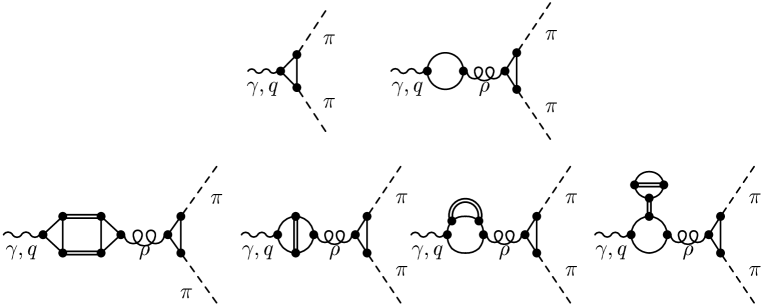
Figure 2.12: Contributions to the pion electromagnetic form factor in the $1/N_{c}$-expansion scheme. The propagator denoted by the curly line corresponds to the $1/N_{c}$-corrected $rho$-meson, while the double lines indicate RPA pions and sigmas.

Evaluating the diagrams of Fig. 2.12 for on-shell pions we notice that the resulting expression for the amplitude displays the same tensorial and isospin structure as that for point-like particles, i.e. it is proportional to $(p^{\mu}-p^{\prime\mu}){\epsilon}_{abc}$ times the electric charge $e$. Here $p$ and $p^{\prime}$ are the four-momenta of the external pions, $a,b$, and $c$ are isospin indices of the pions and the photon. Calculating the ratio of the cross sections we become aware that this common factor and the common phase space factor cancel. We finally obtain for the form factor, $q=-p-p^{\prime}$,

$$|F_{\pi}(q)|^{2}=\frac{1}{4}\,\Big{|}\,g_{\pi qq}^{(0)2}f(p,p^{\prime})\,\Big{(}1-{\tilde{\Pi}}_{\rho}(q){\tilde{D}}_{\rho}(q)\Big{)}\,\Big{|}^{2}~{},$$ (2.22)

where $f(p,p^{\prime})$ is a scalar function appearing in the $\rho\pi\pi$-vertex function (see App. D). Of course, the external pions are to be taken on-shell, i.e. $p^{2}=p^{\prime 2}=m_{\pi}^{2}$ and $p\cdot p^{\prime}=q^{2}/2-m_{\pi}^{2}$. Since a real photon ($q^{2}=0$) should “see” the actual charge of the pion, the form factor should equal unity at $q^{2}=0$. The subtraction performed in Eq. (2.21) guarantees that the $\rho$-meson self energy ${\tilde{\Pi}}_{\rho}$ vanishes at this point. Therefore we have to check whether $|g_{\pi qq}^{(0)2}f(p,p^{\prime})|^{2}=4$ holds for $q^{2}=0$. This can most easily be shown with the help of the Ward-Takahashi identity derived in section 1.5 for the $\rho\pi\pi$-vertex (see Eq. (1.123)). This identity is not directly applicable to our problem since the vertex is not contracted with $q_{\mu}$ in our case. However, this can be handled by using the following relation,

$$\Gamma^{\mu,abc}_{\rho,\pi,\pi}(q,p)=\frac{d\,(q_{\nu}\Gamma^{\nu,abc}_{\rho,\pi,\pi}(q,p))}{d\,q_{\mu}}-q_{\nu}\frac{d\,\Gamma^{\nu,abc}_{\rho,\pi,\pi}(q,p))}{d\,q_{\mu}}~{}.$$ (2.23)

Using the Ward-Takahashi identity, Eq. (1.123), we can write the first term on the r.h.s. of this expression as the derivative of a difference of pion polarization functions in the RPA. Performing the limit $q\rightarrow 0$ and comparing the result for the vertex with the definition of the pion quark coupling constant $g_{\pi qq}^{(0)}$ we deduce

$$g_{\pi qq}^{(0)\,2}f(p,p^{\prime})\Big{|}_{q^{2}=0}=2~{},$$ (2.24)

leading to the desired value for the form factor at $q^{2}=0$.

Figure 2.13: Pion electromagnetic form factor (left panel) and the $\pi\pi$-phase shifts in the vector-isovector channel (right panel) for $\Lambda_{M}=500$ MeV and $g_{v}=1.0g_{s}$ (dashed), $\Lambda_{M}=600$ MeV and $g_{v}=1.6g_{s}$ (solid) as well as $\Lambda_{M}=700$ MeV and $g_{v}=2.4g_{s}$ (dotted) in the $1/N_{c}$-expansion scheme. The other parameter values are taken from Table 2.1. The data points are taken from refs. [72] and [73], respectively.

Our results for $|F_{\pi}|^{2}$ in the $1/N_{c}$-expansion scheme as a function of the center-of-mass energy squared are displayed in the left panel of Fig. 2.13, together with the experimental data [72]. The three theoretical curves are calculated with different values of the meson cutoff, $\Lambda_{M}=500$ MeV (dashed line), $\Lambda_{M}=600$ MeV (solid), and $\Lambda_{M}=700$ MeV (dotted). We have already emphasized that these values for the meson cutoff lie within the small window of cutoff values where we can hope to produce reasonable results. The vector coupling constant $g_{v}$ is chosen such that the maximum of the form factor lies at the right position. The other parameters are taken from Table 2.1. For $\Lambda_{M}=500$ MeV we observe a kink in the form factor slightly above the maximum ascribable to the quark-antiquark threshold at $s=0.63~{}{\rm GeV}^{2}$. Below the kink the form factor drops very steeply due to the sub-threshold attraction in the vector channel. Thus the poor description of the data above the maximum can be attributed to quark-antiquark threshold effects. Therefore we would conclude that our lower boundary for the meson cutoff, determined by the prescription that the threshold lies above the maximum, has not been chosen restrictively enough. However, the behavior of the form factor below the maximum, where threshold effects are less important, indicates that a higher value of the cutoff presumably produces better agreement with the data. Since increasing the cutoff reinforces the mesonic, in this case pionic, fluctuations we expect that with a larger $\Lambda_{M}$ the width of the form factor will be less underestimated. In fact, with a cutoff of $\Lambda_{M}=700$ MeV the width is already noticeably overestimated coming along with a diminished height of the maximum. Below the maximum the description of the data is almost perfect with a cutoff of $\Lambda_{M}=600$ MeV. Above the maximum we certainly miss the detailed structure of the form factor around $s=0.61~{}{\rm GeV}^{2}$ which is due to $\rho-\omega$-mixing, not included in our model. Approaching the threshold at $s=0.80~{}{\rm GeV}^{2}$, effects induced by quarks become more and more important resulting in an underestimation of the data in this region. Probably the overall agreement with the data can be somewhat improved by taking a slightly larger value for $\Lambda_{M}$ but since we are not interested in fine-tuning here, we keep the fit with $\Lambda_{M}=600$ MeV.

Two quantities closely related to the pion electromagnetic form factor are well suited for confirming the consistency of our calculations with experimental data. The first one is the charge radius of the pion, which is defined as

$$\langle{r_{\pi}^{2}}\rangle=6\,\frac{dF_{\pi}}{dq^{2}}\Big{|}_{q^{2}=0}\;.$$ (2.25)

Obviously at $q^{2}=0$ the details of the $\rho$-meson peak are less important than in the higher energy part. A simple pole ansatz for the form factor leads to $\langle{r_{\pi}^{2}}\rangle^{1/2}=\sqrt{6}/m_{\rho}=0.63$ fm [74], a value which is already close to the experimental value of $\langle{r_{\pi}^{2}}\rangle^{1/2}$ = (0.663 $\pm$ 0.006) fm [75]. Our results, $\langle{r_{\pi}^{2}}\rangle^{1/2}=0.59$ fm for $\Lambda_{M}=500$ MeV, $\langle{r_{\pi}^{2}}\rangle^{1/2}=0.61$ fm for $\Lambda_{M}=600$ MeV and $\langle{r_{\pi}^{2}}\rangle^{1/2}=0.66$ fm for $\Lambda_{M}=700$ MeV, also satisfactorily agree with the experimental value. Since this quantity is not very well suited to fix the model parameters, which is clear from the above reasoning, we shall not worry about the fact that for $\Lambda_{M}=700$ MeV, which has been found to be too large to reproduce the data in the region of the maximum, the agreement with the data is almost perfect whereas for lower values of the cutoff the charge radius turns out to be slightly too small.

Figure 2.14: Diagrams contributing to the $\pi\pi$-scattering amplitude: Quark box diagram (left), t- and u-channel $\rho$- or $\sigma$-meson exchange (middle) and s-channel $\rho$-meson exchange (right). Only the latter is taken into account in our calculations.

Other observables are the $\pi\pi$-phase shifts in the vector-isovector channel. We assume here that the dominant contribution to these phase-shifts arise from the s-channel $\rho$-meson exchange, visualized on the r.h.s. of Fig. 2.14. The other processes shown in Fig. 2.14, the direct scattering via quark box or the t- and u-channel exchange of a $\rho$- or a $\sigma$-meson, respectively, are neglected. The result for different values of $\Lambda_{M}$, together with the empirical data [73], is displayed in the right panel of Fig. 2.13. Again, below the $\rho$-meson peak, which is to be understood as the location where the phase shifts equal $90\deg$, the best description of the data is obtained with a cutoff of $\Lambda_{M}=600$ MeV, whereas for higher energies, where threshold effects begin to influence the results for the latter cutoff substantially, $\Lambda_{M}=700$ MeV produces better agreement with the data.

The choice of contributions to the phase shifts has been made on purely phenomenological grounds, motivated by the decisive role of the s-channel $\rho$-meson exchange. In addition to the s-channel $\rho$-meson exchange the direct scattering process via a quark box seems to be a suggestive contribution since it is of leading order in $1/N_{c}$, i.e. Hartree + RPA [76]. Obviously it destroys unitarity of the $S$-matrix if it is not iterated. Because of the non-trivial momentum dependence of the quark box diagram, this would be a very difficult task. On the other hand phase shifts are only properly defined if the $S$-matrix fulfills unitarity. Our evaluation of the phase shifts in the vector-isovector benefits from the dominant role of the s-channel $\rho$-meson exchange which, when taken apart, is not in contradiction to unitarity. In any case, it can be checked that including the quark box diagram leaves the results for the scattering amplitude almost unchanged, thus justifying our assumption. In the scalar-isoscalar channel, on the contrary, we do not expect this pragmatic approach to be as successful. In that case the $t$- and $u$-channel $\sigma$-meson exchange is essential in order to fulfill some of the low-energy theorems. Anyway, the $\sigma$-meson within our model suffers from severe shortcomings which render it senseless to attack the problem of calculating phase shifts. This will be discussed in section 2.8.

Figure 2.15: Real part of the $\rho$-meson polarization function $\tilde{\Pi}_{\rho}$ as a function of the energy $\sqrt{s}$ in the rest frame of the meson. The solid line corresponds to the $1/N_{c}$-expansion scheme with $\Lambda_{M}$ = 600 MeV, the dashed line to the MLA with $\Lambda_{M}$ = 700 MeV. The other parameters are given in Table 2.1 and Table 2.2, respectively.

The preceding presentation of the results in the $1/N_{c}$-expansion scheme offered the possibility to decisively fix a consistent parameter set within this scheme. However, the much more narrow range for variations of the meson cutoff we found for the MLA in the previous section, renders it unlikely that such a fit is possible also in the MLA. In the $1/N_{c}$-expansion scheme we found threshold effects to cause a steep drop in the pion electromagnetic form factor just below this threshold, leading to the conclusion that a constituent quark mass of about 400 MeV, shifting the threshold only slightly above the $\rho$-meson peak in the form factor, is not sufficiently large. This further restricts the possible values for the meson cutoff to a small range just below $\Lambda_{M}=700$ MeV. Hence the only variable parameter to fit the form factor is the vector coupling constant $g_{v}$. In fact, if we take $\Lambda_{M}=700$ MeV, it turns out that we unfortunately run into instabilities in the $\rho$-meson propagator similar to those found in the propagator of the pion (see section 2.5) [42]. This observation is of course independent of the value of $g_{v}$ since it can be detected already in the polarization function $\tilde{\Pi}_{\rho}$.

To this end the real part of the of the $\rho$-meson polarization function $\tilde{\Pi}_{\rho}$ is plotted in Fig. 2.15 as a function of the energy $\sqrt{s}$ in the rest frame of the meson. The MLA result corresponds to the dashed line. For comparison we also show this function in the $1/N_{c}$-expansion scheme, using the ‘best-fit parameters’ given above (solid line).

The “proper” behavior of the polarization function can be derived from what we expect of the inverse propagator. It has to develop a zero for $\sqrt{s}\simeq m_{\rho}$ to produce the well pronounced peak in the form factor. Thus $2g_{v}Re\tilde{\Pi}_{\rho}$ has to become equal to unity for an energy of about 770 MeV. In the $1/N_{c}$-expansion scheme this can easily be achieved by an appropriate choice of the coupling constant since the polarization function is (at least below the quark-antiquark threshold) a steadily rising function. In the MLA, on the contrary, this condition can by no means be fulfilled due to the maximum at $\sqrt{s}\sim 740$ MeV and the subsequent steep drop the polarization function displays. Consequently for a weak coupling, i.e. small $g_{v}$, we observe no zero at all in the inverse propagator whereas for stronger couplings we find two solutions, one at lower energies and one above the maximum. Obviously within those scenarios we would obtain only a very unrealistic description of the $\rho$-meson. Thus we conclude that we did not succeed in performing a fit of the observables in the pion sector, $m_{\pi},f_{\pi}$, and $\langle{\bar{\psi}\psi}\rangle$, simultaneously with properties of the $\rho$-meson in the MLA.

Figure 2.16: Real parts of the RPA contribution $\Pi_{\rho}$ (solid) and the various correction terms to $\tilde{\Pi}_{\rho}$: $\delta\Pi_{\rho}^{(a)}$ (long-dashed), $\delta\Pi_{\rho}^{(b)}$ (dotted), $\delta\Pi_{\rho}^{(c)})$ (short-dashed), and $\delta\Pi_{\rho}^{(d)}$ (dashed-dotted). For all contributions we performed a subtraction, such that they vanish at $\sqrt{s}$ = 0. The left panel corresponds to the $1/N_{c}$-expansion scheme, the right panel to the MLA. The model parameters are the same as in Fig. 2.15.

The cusp in the $\rho$-meson polarization function responsible for the peculiar behavior of the inverse $\rho$-propagator in the MLA looks very similar to that emerging in the inverse pion propagator for large values of the mesonic cutoff, see the discussion in section 2.5. It has also the same origin: the strong momentum dependence of the only negative contribution, diagram $\delta\Pi^{(b)}_{\rho}$. This can be seen from the right panel of Fig. 2.16, where we have separately plotted the various contributions to the polarization function of the $\rho$-meson. On the l.h.s. of Fig. 2.16 the same is shown for the $1/N_{c}$-expansion scheme. One might wonder, why the results in the $1/N_{c}$-expansion scheme permit a reasonable description of the $\rho$-meson, although qualitatively the behavior of diagram $\delta\Pi_{\rho}^{(b)}$, responsible for the unphysical behavior in the MLA, agrees with that in the MLA. However, in the $1/N_{c}$-expansion scheme its contribution is almost cancelled by that of diagram $\delta\Pi^{(d)}_{\rho}$, which is not present in the MLA where the corresponding quark self-energy insertion is selfconsistently absorbed in the modified gap equation (Eq. (1.72)). Thus probably the purely perturbative treatment of both next-to-leading order quark self-energy insertions, $\delta\Pi^{(b)}$ and $\delta\Pi^{(d)}$, within the $1/N_{c}$-expansion scheme helps to suppress unphysical effects. However, we should emphasize that any unphysical behavior we detect here, although observed below the quark-antiquark threshold, is mainly induced by quark effects. In section 2.5 we already noted that in particular the momentum dependence of the real part of $\delta\Pi^{(b)}_{\pi}$ below the threshold is related via dispersion relations to an imaginary part with the “wrong” sign above the threshold. In the same way the real part of all other diagrams below the threshold is influenced by the quark-antiquark continuum. Only digram $\delta\Pi^{(a)}$ is not exclusively governed by effects which can be traced back to the quark-antiquark continuum: Here the imaginary part due to the two-meson intermediate state in a large range of momenta dominates. In the following section we will carry on this discussion in connection with a comparison of these results with those obtained in the static limit.

In any case the results suggest that the unphysical behavior of the polarization function can be at least weakened in energy regions relevant for the description of hadrons by pushing the constituent quark mass further up. This presumption is mainly supported by the steep drop in $\delta\Pi^{(b)}$ occurring only just below the threshold. One might suggest that the constituent quark mass is increased if further intermediate states are included in the model. However, we have seen that it is an extremely difficult task to implement $\rho$- and $a_{1}$-mesons within the present model (see section 2.4.3). In addition the observations made in section 2.5 indicate that we have to cope with an even more severe problem when including vector and axial intermediate states: We observed “restoration” of chiral symmetry if the mesonic fluctuations became too strong. Thus, it seems as if the inclusion of the $\rho$- and $a_{1}$-subspace for the intermediate states would not help without further modifications (or extensions) of the model.

2.7 Comparison with the static limit

This section is devoted to a comparison of the results obtained in the full model with those in the static limit, i.e. the approximation introduced in section 1.6. This approximation is (in vacuum) equivalent to a purely hadronic description, i.e. all quark effects are suppressed. The only reminiscence of the full model can be found in the quark mass dependence of the effective coupling constants. Since the approximations to the MLA and the $1/N_{c}$-expansion scheme do not differ qualitatively from each other, it is completely sufficient for our purpose to restrict the discussion within this section to one of the schemes. We have decided to take the $1/N_{c}$-expansion scheme because only within that scheme we are able to consistently describe the data in the pion sector as well as for the $\rho$-meson.

From the very beginning, we are for two reasons very distrustful of the static limit being a good approximation to the full calculation. First, the estimate of a realistic value of the constituent quark mass within this approximation (see Eq. (1.143)) seems to be in contradiction with the motivation of large quark masses as compared with the relevant momenta, with which we started in section 1.6. In addition indications were found in the previous sections that quark effects are important for the mesonic polarization functions. The estimate performed in section 1.6 can also be applied vice versa: If we insert the parameters of our best fit to the pion electromagnetic form factor in the $1/N_{c}$-expansion scheme (those listed in Table 2.1 for $\Lambda_{M}=600$ MeV) into Eq. (1.142), we obtain a value of $g_{\rho\pi\pi}=9.4$ for the effective $\rho\pi\pi$ coupling constant, which is considerably larger than the value of $g_{\rho\pi\pi}\approx 6$ usually needed in hadronic models to describe the data. Already with $\Lambda_{M}=500$ MeV, which in the full calculation noticeably underestimates the width of the $\rho$-meson, the value of $g_{\rho\pi\pi}\approx 6$ is exceeded by about 40%.

Figure 2.17: The imaginary part of the $1/N_{c}$-corrected $\rho$-meson propagator. The solid line represents the full calculation while the dashed line denotes the static limit.

To compare the static limit with an exact treatment of the $1/N_{c}$-expansion scheme we will look at the imaginary part of the $\rho$-meson propagator which is displayed in Fig. 2.17. The solid line represents a full calculation with $\Lambda_{M}=600$ MeV, the dashed line the corresponding static limit. Since we have fitted the parameters used in the full calculation to the pion electromagnetic form factor, the maximum of the corresponding imaginary part is close to the $\rho$-meson mass of 770 MeV whereas this does not necessarily need to be the case in the static limit. In fact, the peak in the static limit is much broader and shifted to higher energies. Another obvious difference is the existence of the quark-antiquark threshold at $\sqrt{s}=892$ MeV in the full model which is not present in the static limit since within that approximation all quark effects are suppressed.

For a better understanding of this intriguingly different behavior already below the unphysical threshold we also compare the real and imaginary parts of the corresponding self-energies (Fig. 2.18). Note that the imaginary part in this region is exclusively generated by the decay process $\rho\rightarrow\pi\pi$. Differences in the imaginary part therefore directly reflect the non-trivial momentum dependence of the quark loops in the meson-meson vertices. They become important only near the threshold. For $\sqrt{s}\mathrel{\raise 1.29167pt\hbox{$<$\kern-7.5pt\lower 4.30554pt\hbox{$\sim$}}}800$ MeV the two curves almost coincide. In the real part the differences are much larger. Coincidence of the two curves can hardly be acknowledged up to $\sqrt{s}\sim 400$ MeV. The real part in the static limit is obviously much less attractive than that in the full calculation. Besides, the slope of the curve is much steeper in the full calculation, which explains the broadening and the shift to higher energies of the peak in the $\rho$-meson propagator as shown in Fig. 2.17. As already emphasized several times, the real part below the threshold is, via dispersion relations, related to the entire imaginary part including that above the threshold. Hence the discrepancies between the static limit and the full model here not only reflect the momentum dependence of the quark loops contained in the vertices but additionally indirect effects arising from quark decay channels.

The only conclusion we can draw from the preceeding discussion is that quark effects are indeed important. At this point one might argue that one has to distinguish between “physical quark effects”, for instance those modifying the point-like structure of the meson-meson vertices, and unphysical quark effects leading to unconfined quarks. However, these two types of effects cannot be considered separately since they are linked to each other via dispersion relations. This is related to a rather fundamental question, namely whether “physical quark effects” exist at all. Of course, at sufficiently high energies quarks should be the relevant degrees of freedom which in one way or another influence hadronic properties. An approach like QCD sum rules [77] in principle offers the possibility to map at least different energy regions. But in any case an explanation of this influence requires first the understanding of quark confinement itself.

Our scheme can only exemplify how a hadronic model emerges naturally from the underlying quark structure provided that the necessary degrees of freedom are included. This can be seen nicely from the low energy region where the static limit almost coincides with the exact treatment of our model.

Figure 2.18: The real part (left) and the imaginary part (right) of the $1/N_{c}$-corrected $\rho$-meson self-energy, multiplied by $-2g_{v}$. The solid line represents the full calculation, while the dashed line indicates the static limit.

2.8 Results for the sigma-meson

Figure 2.19: The imaginary part of the “improved ” $\sigma$-meson propagator, $\tilde{D}_{\sigma}$ in the $1/N_{c}$-expansion scheme (left) and in the MLA (right) for $\Lambda_{M}=600$ MeV.

The sigma-meson is not a very well established particle in nature. In the “Review of Particle Physics” [50] we read concerning the $\sigma$: “The interpretation of this entry as a particle is controversial.” The mass of this “particle” lies between 400 and 1200 MeV with a width of the same magnitude, 600-1000 MeV. However, in chiral models where chiral symmetry is linearly realized, like the NJL model, it inevitably accompanies the pion as its chiral partner. Most of the models deal with a sharp $\sigma$-particle on tree-level. However, due to its strong coupling to a two-pion state the $\sigma$-meson is significantly broadened. Within a linear sigma model approach this notion has been successfully applied to predict not only a broad resonance in vacuum but also its sharpening due to partial restoration of chiral symmetry in medium (see Schuck et al. [78] and references therein). The description of the $\sigma$-meson in the NJL model in the standard Hartree + RPA scheme is certainly not suitable to obviate this problem. Within that approximation the $\sigma$-meson is an (almost) sharp particle, located at the $q\bar{q}$-threshold or just above. Thus, the inclusion of mesonic fluctuations, in particular pionic ones, in the $1/N_{c}$-expansion scheme or the MLA seems to be a promising starting point to improve the phenomenology of the $\sigma$-meson within the NJL model.

Figure 2.20: The real part (left) and the imaginary part (right) of the various corrections terms to the $\sigma$-meson polarization function, multiplied by $2g_{s}$, in the $1/N_{c}$-expansion scheme (upper panel) and in the MLA (lower panel): total polarization function $\tilde{\Pi}_{\sigma}$ (solid line), $\delta\Pi_{\sigma}^{(a)}$ (long dashed line), $\delta\Pi_{\sigma}^{(b)}$ (dotted line), $\delta\Pi_{\sigma}^{(c)}$ (short dashed line), and $\delta\Pi_{\sigma}^{(d)}$ (dashed-dotted). Note that the contribution of $\delta\Pi^{(d)}_{\sigma}$ is missing in the MLA.

Actually, in both schemes, the $1/N_{c}$-expansion scheme and the MLA, the $\sigma$-meson is substantially broadened above the two-pion threshold as can be inferred from the left and right panel of Fig. 2.19, respectively, where the imaginary part of the $\sigma$-propagator $\tilde{D}_{\sigma}(s)$ as a function of the energy $\sqrt{s}$ in the rest frame of the meson is displayed. For the $1/N_{c}$-expansion scheme the calculation has been performed with $\Lambda_{M}=600$ MeV and the corresponding “best fit” parameter set listed in Table 2.1. In the MLA, where we did not succeed in performing a consistent fit, we also took $\Lambda_{M}=600$ MeV together with the parameters shown for that value of the cutoff in Table 2.2. In the MLA we find, in addition to the broadening above the two-pion threshold, a sharp peak just below that threshold which would be a $\delta$-function if we had not introduced by hand some small but nonzero imaginary part. The origin of this peak will become clear from the behavior of the polarization function itself.

The left panels of Fig. 2.20 show the real parts of the different contributions to the $\sigma$-meson polarization function as a function of $s$. The momentum dependence of the real part is mainly caused by the contribution arising from $\delta\Pi_{\sigma}^{(a)}$ (long-dashed line), i.e. the correction term containing the two-pion intermediate state. Below the $q\bar{q}$-threshold this term is in fact the only one producing a nonvanishing imaginary part. This imaginary part is shown on the r.h.s. of Fig. 2.20. These features are common for the $1/N_{c}$-expansion scheme and the MLA.

Figure 2.21: Real part of the inverse $\sigma$-meson propagator. (Left): $g_{\sigma qq}^{(0)2}\tilde{D}_{\sigma}^{-1}(s)$ in the $1/N_{c}$-expansion scheme with $\Lambda_{M}=600$ MeV (solid line) and in the static limit (short-dashed line), $g_{\sigma qq}^{(0)2}D_{\sigma}^{-1}(s)$ in RPA (long-dashed line), $s-4m_{H}^{2}$ (dotted line), and the corresponding linear sigma-model result by Aouissat et al. [79] (dashed-dotted line). (Right): $1/N_{c}$-expansion scheme with $\Lambda_{M}=600$ MeV (dashed), $\Lambda_{M}=600$ MeV (solid), and $\Lambda_{M}=900$ MeV (dotted).

This rather encouraging result, at least for the $1/N_{c}$-expansion scheme, is spoiled, however, if we investigate the analytic properties of the propagator more closely. Recalling that the propagator acquires a pole if $2g_{s}\tilde{\Pi}_{\sigma}(s)$ becomes equal to unity, one understands the existence of the sharp peak in the $\sigma$-meson propagator in MLA. In the $1/N_{c}$-expansion scheme, on the other hand, the existence of a pole is not as obvious. In the time-like region we find no pole at all, explaining the smaller scale of the imaginary part of the propagator as compared with that in the MLA (Fig. 2.19). We only guess from the slope of the polarization function at $s=0$ that this might very well occur for negative, i.e. space-like, $s$. This would of course be a very disturbing unphysical feature of the $\sigma$-propagator. Unfortunately we cannot support this guess by explicit results: Since we work in the rest frame of the mesons, we are not able to perform calculations for space-like momenta.

However, another fact which can already be deduced from the value of the real part of the polarization function at $s=0$ corroborates the doubts concerning our results for the $\sigma$-meson: The sign of the inverse propagator at $s=0$ differs from what we except from a comparison with a free propagator $1/(s-m_{\sigma}^{2})$. On the l.h.s. of Fig. 2.21 we have displayed the inverse $\sigma$-propagator as it emerges from the $1/N_{c}$-expansion scheme (solid line), in the static limit (short-dashed line), the free one with an arbitrarily chosen mass of $m_{\sigma}=2m_{H}$ (dotted line) and for comparison the RPA one (long-dashed line) and the result obtained by Aouissat et al. [79] (dashed-dotted line). Note that we have normalized the results in RPA and in the $1/N_{c}$-expansion scheme to the RPA $\sigma$-quark coupling constant $g_{\sigma qq}^{(0)2}$. In the vicinity of $s$=0 the slope of the various inverse propagators agrees at least concerning the sign, while the function itself has positive values in the $1/N_{c}$-expansion scheme and negative ones in the two other cases. This behavior is basically not altered if we vary the mesonic cutoff. This can be inferred from the right panel of Fig. 2.21 where we have plotted the inverse $\sigma$-propagator in the $1/N_{c}$-expansion scheme using different values of $\Lambda_{M}$ while all other parameters are kept constant. The effect of varying the cutoff is mainly to shift the entire curve up or down. The shape remains almost the same. For small values of $\Lambda_{M}$, cf. the dashed line with $\Lambda_{M}=200$ MeV, we encounter the even more peculiar situation, which has already been observed in the MLA (see Fig. 2.20), where we have two zeros in the real part of the inverse $\sigma$-propagator in the time-like region, one below the two-pion threshold at about 280 MeV and one above. With increased cutoff the curve is first shifted upwards, then, if the cutoff exceeds $\Lambda_{M}\mathrel{\raise 1.29167pt\hbox{$>$\kern-7.5pt\lower 4.30554pt\hbox{$\sim$}}}900$ MeV it begins to move downwards again. Nevertheless it seems to be hopeless that we can obtain a more realistic description of the $\sigma$-propagator for very large values of the cutoff. On the one hand, if the shape of the curve is not altered, we cannot avoid finding finally two poles in the time-like region instead of one. On the other hand the investigations in the previous sections, concerning the pion and the $\rho$-meson, render it plausible that we run into instabilities when applying such large values for the cutoff, besides completely failing to describe the data in the pion and $\rho$-meson sector.

Figure 2.22: Example for contributions to the $\sigma$-meson polarization function similar to those included in Ref. [79] (see text).

Till now each unphysical phenomenon we detected could be ascribed to strong quark effects. This is not true for the present case. The left panel of Fig. 2.21 also displays the result in the static limit (short-dashed line), where all quark effects are suppressed, which shows essentially the same behavior, at least in the low-energy region, as the calculation in the $1/N_{c}$-expansion scheme. This leads us to the conclusion that the strong attraction of the two-pion state in the scalar-isoscalar channel is responsible for this behavior. It is therefore suggestive that it can be mended by imitating the terms which produce reasonable results in a linear sigma-model calculation by Aouissat et al. [79] (see l.h.s. of Fig. 2.21, dashed-dotted line). The RPA used by the authors of Ref. [79] consists of iterating the entire pion-pion scattering amplitude in the scalar-isoscalar channel for the self-energy of the $\sigma$-meson. In our case this would mainly correspond to terms like those presented in Fig. 2.22. Terms of that type would have been included in the “improved” polarization function if we had applied the $\Phi$-derivable method discussed in section 1.3.3. The scattering kernel of the quark-antiquark Bethe-Salpeter equation visualized in Fig. 1.8 precisely contains those non-local contributions necessary to generate the desired $\sigma$-meson polarization function. In any case, we resigned to pursue that scheme further because it is very difficult to handle due to the non-local structure, which already shows up in the modified gap equation (cf. Fig. 1.8).

Chapter 3 Results at nonzero temperature

It is commonly believed that chiral symmetry, which is spontaneously broken in vacuum, gets restored at high temperatures as well as at high densities. For a recent review on the present view of the QCD phase diagram see Ref. [25]. In wide ranges of densities and temperatures this notion is, however, based on model calculations for lack of fundamental knowledge. Only at low temperatures and low densities model independent results can be obtained by considering a gas of pions or a gas of pions and nucleons, respectively. Pions are the dominant degrees of freedom in that range because of their small mass as compared with other possible degrees of freedom. At zero chemical potential, i.e. zero density, lattice calculations provide us with results also in the vicinity of the phase transition, but at nonzero chemical potential no realistic lattice results exist. Thus in that region we have to rely entirely on model calculations.

One of the models which has been applied by many authors to study the effects of (partial) chiral symmetry restoration at nonzero temperature and density on various quantities, in particular the quark condensate as the order parameter of chiral symmetry and properties of mesons, is the NJL model. Most of these investigations have been performed in the standard approximation scheme, i.e. Hartree + RPA (see e.g. [17, 18, 19, 20]). The main drawback of these examinations is certainly the unphysical nature of the degrees of freedom, deconfined quarks, taken into account to describe the thermodynamical properties of the system. The presence of unphysical degrees of freedom is not the only weak point of these studies. In addition, the relevant degrees of freedom, at low temperatures and densities mainly pions, are completely missing such that, for instance, the model independent results within that range cannot be reproduced by these calculations. Hence, although the fundamental problem of lack of confinement cannot be overcome, we can hope to improve the results by introducing mesonic degrees of freedom within an approximation beyond Hartree + RPA, i.e. in the $1/N_{c}$-expansion scheme or the MLA. Since both schemes do not contain any nucleons, essential ingredients at nonzero densities, we will restrict our examinations in the $1/N_{c}$-expansion scheme and the MLA to nonzero temperatures but zero density.

3.1 Results in Hartree approximation + RPA

Before we present first results at nonzero temperature in the $1/N_{c}$-expansion scheme and the MLA, we will briefly review the results in the standard approximation scheme, namely Hartree + RPA. To this end we first have to generalize the formalism presented in Chapter 1 to nonzero temperature and chemical potential. We will keep the latter since it enters into the expressions in almost the same way as nonzero temperature. In principle we can choose between two different methods to deal with thermodynamic properties of the system: the imaginary time or Matsubara formalism (see e.g. [80]), and the real time formalism (see e.g. [81]). Within this paper we will adopt the Matsubara formalism for simplicity. We should remark that it is not applicable to determine the temperature dependence of the mesonic properties in the $1/N_{c}$-expansion scheme or the MLA. This requires the analytic continuation of functions only known numerically for a finite number of points, which cannot be done uniquely. In any case we will restrict the later discussion on the quark condensate which is a static quantity and can therefore be treated within the Matsubara formalism.

The basics of the Matsubara formalism can be found in textbooks, e.g. in Ref. [80]. In App. E we summarize the Feynman rules we obtain starting from the Lagrangian in Eq. (1.1). The resulting expressions at nonzero temperature and chemical potential $\mu$ can be written formally in almost the same way as in vacuum if we replace the integration over energy in the vacuum expressions by a sum over fermionic or bosonic Matsubara frequencies $i\omega_{n}$, i.e.

$$i\int\frac{d^{4}k}{(2\pi)^{4}}f(k)\rightarrow-T\sum_{n}\int\frac{d^{3}k}{(2\pi)^{3}}f(i\omega_{n},\vec{k})~{}.$$ (3.1)

If we have a nonvanishing chemical potential for the quarks, $\mu$ should be added to the fermionic Matsubara frequency in all expressions, i.e. $i\omega_{n}\rightarrow i\omega_{n}+\mu$. The replacement prescription in Eq. (3.1) can be applied to define the analogue to the elementary integrals in vacuum, e.g.

$$I(p) = \int\frac{d^{4}k}{(2\pi)^{4}}\frac{1}{(k^{2}-m^{2}+i{\epsilon})((k+p)^{2}-m^{2}+i{\epsilon})}\rightarrow$$

$$I(i\omega_{l},\vec{p}) = iT\sum_{n}\int\frac{d^{3}k}{(2\pi)^{3}}\frac{1}{((i\omega_{n}+\mu)^{2}-\vec{k}^{2}-m^{2})((i\omega_{n}+\mu+i\omega_{l})^{2}-(\vec{k}+\vec{p})^{2}-m^{2})}~{}.$$

Note that the expressions at nonzero $T$ and $\mu$ depend separately on energy and three-momentum because a preferred frame of reference exists in the heat bath. This simplifies our notation: the second argument enables us to clearly distinguish vacuum quantities from their medium analogues. Functions with one argument, e.g. $p$, denote vacuum quantities, whereas functions with two arguments, e.g. $i\omega_{l},\vec{p}$, are the corresponding in-medium quantities, such that we can use the same symbols to mark analogous quantities. The only exception are static quantities which do not depend on momentum at all. There we will add a suffix $T$, e.g. the quark condensate in medium will be denoted by $\langle{\bar{\psi}\psi}\rangle_{T}$.

Figure 3.1: $m_{\pi}^{(0)}$ (solid line) and $m_{\sigma}^{(0)}$ (dashed) as a function of temperature in the chiral limit (left panel) and with $m_{0}=6.13$ MeV (right panel). For the remaining parameters see Table 2.1 for $\Lambda_{M}=0$.

Figure 3.2: Imaginary part of the $\rho$-meson (solid line) and $a_{1}$-meson (dashed line) propagator in RPA for different temperatures.

The proportionality of the constituent quark mass to the quark condensate in the Hartree approximation, see Eq. (1.6), suggests that this quark mass is strongly influenced by medium effects in the vicinity of the phase transition. In fact, the medium analogue of the gap-equation, Eq. (1.2),

$$m_{HT} = m_{0}-2g_{s}4N_{c}N_{f}m_{HT}T\sum_{n}\int\frac{d^{3}k}{(2\pi)^{3}}\frac{1}{(i\omega_{n}+\mu)^{2}-E^{2}}$$ (3.3)

$$= m_{0}+2g_{s}4N_{c}N_{f}m_{HT}I_{1T}~{},$$

with $E=\sqrt{\vec{k}^{2}+m_{HT}^{2}}$ and $\omega_{n}=(2n+1)\pi T$ being fermionic Matsubara frequencies, reveals the $T$ as well as the $\mu$ dependence of the constituent quark mass $m_{HT}$. The self-consistent solutions of this equation correspond to extrema of the thermodynamic potential

$$\Omega^{(0)}(m_{T},T,\mu)=-2N_{c}N_{f}T\sum_{n}\int\frac{d^{3}k}{(2\pi)^{3}}\ln\Big{(}\frac{E^{2}-(i\omega_{n}+\mu)^{2}}{m_{0}^{2}+\vec{k}^{2}-(i\omega_{n}+\mu)^{2}}\Big{)}+\frac{(m_{T}-m_{0})^{2}}{4g_{s}}+const.~{},$$ (3.4)

which can be employed to study the phase structure of the system. In the above formula we set $g_{v}=0$ for simplicity. For details how to include vector interactions see e.g. Ref. [82, 83]. In this approximation the NJL model exhibits a second order phase transition at $\mu=0,T\neq 0$ with a critical temperature of $T_{c}\approx 150-200$ MeV and, depending strongly on the choice of parameters [83], a second or a first order phase transition at $T=0,\mu\neq 0$ with a critical chemical potential of the same order of magnitude as the constituent quark mass in vacuum, $\mu_{c}\approx 300-400$ MeV.

In addition, the properties of the mesons in the RPA are modified by medium effects. The polarization functions for the RPA pion and the $\sigma$-meson read

$$\Pi_{\sigma}(i\omega_{l},\vec{p}) = 4iN_{c}N_{f}I_{1T}-2iN_{c}N_{f}((i\omega_{l})^{2}-\vec{p}^{2}-4m_{T}^{2})I(i\omega_{l},\vec{p})$$

$$\Pi_{\pi}(i\omega_{l},\vec{p}) = 4iN_{c}N_{f}I_{1T}-2iN_{c}N_{f}((i\omega_{l})^{2}-\vec{p}^{2})I(i\omega_{l},\vec{p})~{},$$ (3.5)

with $\omega_{l}=2l\pi T$ being bosonic Matsubara frequencies. Below the phase transition the integral $I_{1T}$ can again be replaced with the help of the gap equation Eq. (3.3) (cf. Eqs. (B.2) and (B.3)). The $\rho$-meson and the $a_{1}$-meson are a little more difficult to handle since we have to keep in mind, that, although the four-dimensional tranverse structure of the corresponding polarization functions is preserved in medium, we have to distinguish between a three-dimensional longitudinal and a three-dimensional transverse part. This will be explained in more detail in App. C.

Although the thermodynamics within this approximation is exclusively driven by unphysical degrees of freedom, deconfined quarks, some features of chiral symmetry restoration can nicely be illustrated. One example is the degeneracy of the spectral functions of the chiral partners, i.e. $\pi$ and $\sigma$ as well as $\rho$ and $a_{1}$, above the phase transition can be mentioned here. For the $\pi$-$\sigma$-system this can be inferred from Fig. 3.1 where the masses of pion and $\sigma$-meson as a function of temperature for $\mu=0$ are displayed. For parameters we chose our standard RPA parameter set. This leads to a critical temperature of $T_{c}=164.4$ MeV. In the chiral limit (left panel) the mass of the pion, denoted by the solid line, vanishes below the phase transition. Away from the chiral limit the pion mass, although non-vanishing, remains almost constant up to $T\approx T_{c}$. In both cases the mass of the $\sigma$-meson (dashed line) decreases with temperature, approaching zero at $T_{c}$ in the chiral limit, and increasing again above the phase transition. Away from the chiral limit pion and $\sigma$ mass do not exactly coincide at (and above) $T_{c}$. For the $\rho$-$a_{1}$-system it is not sufficient to consider masses alone since both, the $\rho$- and the $a_{1}$-meson, lie well above the $q\bar{q}$-threshold already for temperatures $T\ll T_{c}$. In Fig. 3.2 we have therefore displayed the imaginary part of the propagators for $T=0$, $T=.61T_{c}$ and $T=.99T_{c}$. Obviously these imaginary parts coincide for $T=T_{c}$ in the chiral limit. We have to emphasize again that these results can only serve as an illustration. Among other points the observation that the $\rho$- and the $a_{1}$-meson lie above the $q\bar{q}$-threshold over wide temperature ranges reveals the unphysical nature of these results.

3.2 Quark condensate at $T\neq 0$ beyond mean field

Within this section we will study the behavior of the quark condensate at nonzero temperature (and $\mu=0$) in the $1/N_{c}$-expansion scheme and the MLA. At the beginning of chapter 3 we expressed the hope that at least the low-temperature behavior can be improved considerably as compared with the Hartree + RPA scheme by including mesonic fluctuations within the $1/N_{c}$-expansion scheme or the MLA. To support this we will first compare the low-temperature behavior we obtain with the expectations from model independent considerations. Within this section we will again neglect fluctuations of $\rho$- or $a_{1}$-mesons.

3.2.1 Low-temperature behavior

Model independent results for the quark condensate can be obtained by a strict low-temperature expansion in chiral perturbation theory. In the chiral limit and at vanishing baryon density this reads [44]

$$\langle{\bar{\psi}\psi}\rangle_{T}=\langle{\bar{\psi}\psi}\rangle\Big{(}1-\frac{T^{2}}{8f_{\pi}^{2}}-\frac{T^{4}}{384f_{\pi}^{4}}+\dots\Big{)}~{}.$$ (3.6)

Here $\langle{\bar{\psi}\psi}\rangle$ denotes the quark condensate at zero temperature. The term proportional to $T^{2}$ arises from a pure (massless) pion gas. It can be derived by considering the pressure of a free pion gas,

$$p_{\pi}=-3T\int\frac{d^{3}k}{(2\pi)^{3}}\ln(1-e^{-E_{\pi}/T})~{},$$ (3.7)

where $E_{\pi}=\sqrt{\vec{k}^{2}+m_{\pi}^{2}}$. The quark condensate is in general given as the negative of the derivative of the total pressure with respect to the current quark mass. Assuming that for small $T$ the change of the quark condensate with temperature is determined by the pion gas and using the GOR relation, Eq. (1.80), we can express the quark condensate as follows:

$$\langle{\bar{\psi}\psi}\rangle_{T}=\langle{\bar{\psi}\psi}\rangle+\delta\langle{\bar{\psi}\psi}\rangle_{T} = \langle{\bar{\psi}\psi}\rangle+\frac{\langle{\bar{\psi}\psi}\rangle}{f_{\pi}^{2}}\frac{\partial p_{\pi}}{\partial m_{\pi}^{2}}$$ (3.8)

$$= \langle{\bar{\psi}\psi}\rangle-\frac{\langle{\bar{\psi}\psi}\rangle}{f_{\pi}^{2}}\frac{3}{2}\int\frac{d^{3}k}{(2\pi)^{3}}\frac{1}{E_{\pi}}\frac{1}{1-e^{-E_{\pi}/T}}~{}.$$

In the chiral limit the integral in the last line of the above expression can be evaluated analytically to give the $T^{2}$-term in Eq. (3.6). The higher-order terms in addition contain interactions between the pions. In the chiral limit it is not astonishing that the massless Goldstone bosons, the pions, are the dominant degrees of freedom at low temperatures. Thus we expect at least the $T^{2}$-term to reflect only the underlying chiral symmetry and not any model specific contributions. However, it can be shown [44] that aside from the $T^{2}$- also the $T^{4}$-term of this expansion follows from chiral symmetry alone. This implies that every model which exhibits chiral symmetry, among others the NJL model, should in principle show the same behavior up to $T^{4}$. In contrast an expansion of the quark condensate in Hartree approximation [20, 55],

$$\langle{\bar{\psi}\psi}\rangle^{(0)}_{T}=\langle{\bar{\psi}\psi}\rangle^{(0)}\Big{(}1-\frac{(2m_{H}T)^{3/2}}{\pi^{3/2}\langle{\bar{\psi}\psi}\rangle^{(0)}}e^{-\frac{m_{H}}{T}}+\dots\Big{)}~{},$$ (3.9)

obviously does not reproduce these terms. There exists a very simple argument [45] why the Hartree approximation is not suited to reproduce these terms: From the fact that $f_{\pi}$ is of the order $\sqrt{N_{c}}$ we gather that the $T^{2}$-term is of the order $1/N_{c}$ and the $T^{4}$-term of the order $1/N_{c}^{2}$. Remembering that the Hartree approximation corresponds to the leading order in an $1/N_{c}$-expansion we immediately see that this approximation must fail in the desired low-temperature behavior. This reasoning also reveals that by extending the calculations to next-to-leading order in $1/N_{c}$ we will at least be able to reproduce the $T^{2}$-term [42]. Although the MLA does not correspond to an expansion in orders of $1/N_{c}$ the $T^{2}$-term can also be reproduced within that approximation scheme [45] because it contains all $1/N_{c}$-correction terms in next-to-leading order. We will now proceed with demonstrating this first for the $1/N_{c}$-expansion scheme, and then for the MLA.

Using the notations introduced in the previous section for the temperature dependent quantities, we can write the quark condensate in next-to-leading order in $1/N_{c}$ in almost the same way as in vacuum (see Eqs. (1.6) and (1.32),

$$\langle{\bar{\psi}\psi}\rangle_{T}=\langle{\bar{\psi}\psi}\rangle^{(0)}_{T}+\delta\langle{\bar{\psi}\psi}\rangle_{T}=-\frac{m_{HT}-m_{0}}{2g_{s}}-\frac{D_{\sigma}(0,0)\Delta_{T}}{2g_{s}}~{}.$$ (3.10)

From Eq. (3.9) we conclude that to order $T^{2}$ thermal effects in the leading-order term $\langle{\bar{\psi}\psi}\rangle^{(0)}$ can be neglected. In the same way one can reason that the temperature dependence of the $\sigma$-propagator does not contribute. Thus we are left with an expansion of $\Delta_{T}$ at low temperatures. $\Delta_{T}$ is explicitly given by

$$\Delta_{T} = 4iN_{c}N_{f}\ m_{T}T\int\frac{d^{3}p}{(2\pi)^{3}}\sum_{l}{\Big{\{}}$$ (3.11)

$$\hskip 65.44142ptD_{\sigma}(i\omega_{l},\vec{p})(2I(i\omega_{l},\vec{p})+I(0,0)-((i\omega_{l})^{2}-\vec{p^{2}}-4m_{T}^{2})K(i\omega_{l},\vec{p}))$$

$$\hskip 56.9055pt+D_{\pi}(i\omega_{l},\vec{p})\ (\;3I(0,0)\;-\;3((i\omega_{l})^{2}-\vec{p}^{2})\ K(i\omega_{l},\vec{p})\;){\Big{\}}}~{},$$

where $\omega_{l}$ are bosonic Matsubara frequencies. If standard techniques are used the sum over the Matsubara frequencies in Eq. (3.11) can be converted into a contour integral [80], where $C$ is a contour encircling the imaginary axis in the positive sense, see Fig. 3.3,

$$\Delta_{T} = 4iN_{c}N_{f}\ m_{T}\frac{1}{2\pi i}\int\frac{d^{3}p}{(2\pi)^{3}}\int_{C}\frac{dz}{e^{z/T}-1}{\Big{\{}}D_{\pi}(z,\vec{p})\ (3I(0,0)-3(z^{2}-\vec{p}^{2})\ K(z,\vec{p}))$$ (3.12)

$$\hskip 51.21504pt+D_{\sigma}(z,\vec{p})\ (2\ I(z,\vec{p})+I(0,0)-(z^{2}-\vec{p^{2}}-4m_{T}^{2})\ K(z,\vec{p})){\Big{\}}}~{}.$$

One proceeds by deforming the contour $C$, first to $C^{\prime}$, then to $C^{\prime\prime}$, in such a way that only the

Figure 3.3: Contours $C$, $C^{\prime}$ and $C^{\prime\prime}$ for the evaluation of $\Delta_{T}$. The poles at the Matsubara frequencies and at the pion energy are explicitly marked as well as the quark-antiquark cuts.

poles of the addends in Eq. (3.11) contribute. In our case we encounter poles at

$$z=\pm\sqrt{\vec{p}^{2}+m_{\pi}^{2(0)}}\equiv\pm E_{\pi}$$

and cuts for

$$z<-\sqrt{4m_{HT}^{2}+\vec{p}^{2}}\quad{\rm and}\quad z>\sqrt{4m_{HT}^{2}+\vec{p}^{2}}~{}.$$

The resulting contour $C^{\prime\prime}$ is also shown in Fig. 3.3. In the evaluation this contour integration each pole at $z=z_{p}$ is weighted with a factor $1/(e^{z_{p}/T}-1)$. Thus at low temperatures the lowest-lying pion pole at $z=\pm E_{\pi}$ gives the main contribution. Subtracting the vacuum part it can be expressed in the following way:

$$(\Delta_{T}-\Delta)_{\pi}=-4iN_{c}N_{f}\ m\int\frac{d^{3}p}{(2\pi)^{3}}\frac{2}{e^{E_{\pi}/T}-1}{\rm Res}{\Big{\{}}D_{\pi}(E_{\pi},\vec{p})\ (3I(0,0)-3(E_{\pi}^{2}-\vec{p}^{2})\ K(E_{\pi},\vec{p}))\Big{\}}~{}.$$ (3.13)

The exponential suppression of the other contributions is certainly the stronger the lower the pion mass is as compared with two times the constituent quark mass $m_{HT}$. In the chiral limit we can therefore approximate $\Delta_{T}$ for low temperatures by the pionic contribution

$$\Delta_{T}-\Delta=4N_{c}N_{f}\ m\int\frac{d^{3}p}{(2\pi)^{3}}\frac{2}{e^{|\vec{p}|/T}-1}{\Big{\{}}\frac{3}{2|\vec{p}|2N_{c}N_{f}}{\Big{\}}}~{}.$$ (3.14)

This integral can be evaluated analytically and we obtain

$$\Delta_{T}-\Delta=m\,{\frac{T}{2}}^{2}~{}.$$ (3.15)

Up to now we have shown that the changes of the quark condensate for low temperatures are indeed proportional to $T^{2}$ in the $1/N_{c}$-expansion scheme. We are left with a comparison of the coefficients in Eqs. (3.6) and (3.10), respectively. In the chiral limit the vacuum $\sigma$-meson propagator can be expressed with the help of the leading-order pion decay constant as, (cf. Eqs. (B.4) and (2.10)),

$$D_{\sigma}(0)=-\frac{1}{4f_{\pi}^{2(0)}}~{}.$$ (3.16)

Inserting this expression together with Eq. (1.6) for the leading order quark condensate and Eq. (3.15), evaluated at the Hartree mass, into Eq. (3.10) we finally arrive at the following expression for the quark condensate in next-to-leading order in $1/N_{c}$ at low temperatures:

$$\langle{\bar{\psi}\psi}\rangle_{T}=\langle{\bar{\psi}\psi}\rangle-\langle{\bar{\psi}\psi}\rangle^{(0)}\frac{T^{2}}{8f_{\pi}^{2(0)}}~{}.$$ (3.17)

A comparison with Eq. (3.6) shows that the coefficients in front of the $T^{2}$-term are similar but not identical. In the $1/N_{c}$-expansion scheme the leading-order quantities, $\langle{\bar{\psi}\psi}\rangle^{(0)}$ and $f_{\pi}^{(0)}$, determine the coefficient in contrast to $\langle{\bar{\psi}\psi}\rangle$ and $f_{\pi}$ in Eq. (3.6). On the one hand this simply reflects the fact that we only get the lowest order contribution to this coefficient by expanding the quark condensate up to next-to-leading order in $1/N_{c}$. On the other hand it can be understood from physical arguments: The $1/N_{c}$-corrections to the quark condensate consist of fluctuating RPA mesons. Hence the low temperature behavior within the $1/N_{c}$-expansion scheme is driven by excited RPA pions and consequently quantities corresponding to the RPA pions.

For the MLA, a similar result has been derived in Ref. [45]. With the preceding results this derivation is easily comprehensible. In the chiral limit the quark condensate in the MLA, cf. Eq. (1.75), is proportional to the quark mass $m^{\prime}_{T}$,

$$\langle{\bar{\psi}\psi}\rangle=-\frac{m^{\prime}_{T}-m_{0}}{2g_{s}}~{},$$ (3.18)

where $m^{\prime}_{T}$ is a solution of the modified gap equation, cf.Eq. (1.72),

$$m^{\prime}_{T}=m_{0}+\Sigma_{HT}(m^{\prime}_{T})-2g_{s}\Delta_{T}(m^{\prime}_{T})~{}.$$ (3.19)

This equation implicitly defines the temperature dependence of $m^{\prime}_{T}$ and therefore also that of the quark condensate. To obtain the $T^{2}$-dependence we will now take the derivative of Eq. (3.19) with respect to $T^{2}$ at $T=0$ and solve this for $dm^{\prime}_{T}/dT^{2}$, i. e.

$$\frac{dm^{\prime}_{T}}{dT^{2}}\Big{|}_{T=0} = \frac{\partial(\Sigma_{HT}-2g_{s}\Delta_{T})}{\partial T^{2}}\Big{|}_{T=0}(1-\frac{\partial(\Sigma_{H}-2g_{s}\Delta)}{\partial m^{\prime}})^{-1}$$ (3.20)

$$= -2g_{s}\frac{m^{\prime}}{2}(1-\frac{\partial(\Sigma_{H}-2g_{s}\Delta)}{\partial m^{\prime}})^{-1}~{},$$

where in the last step we have employed Eq. (3.15) and used the fact that the derivative of $\Sigma_{HT}$ with respect to $T^{2}$ vanishes for $T=0$. From the definition of the inverse meson propagators in the MLA in section 1.3.3 it is obvious that the derivative of the quark self energy with respect to the quark mass is related to the $\sigma$-meson polarization function $\tilde{\Pi}_{\sigma}(0)$. Thus the above expression can be written in terms of the $\sigma$-meson propagator for vanishing momentum

$$\frac{dm^{\prime}_{T}}{dT^{2}}\Big{|}_{T=0}=\tilde{D}_{\sigma}(0)\frac{m^{\prime}}{2}~{}.$$ (3.21)

The authors of Ref. [45] argue that the leading order piece in $1/N_{c}$ of the above expression is the RPA $\sigma$-meson propagator which in turn can be expressed with the pion decay constant to that order. Consequently the authors find

$$\langle{\bar{\psi}\psi}\rangle_{T}=\langle{\bar{\psi}\psi}\rangle\Big{(}\,1\;-\;\frac{T^{2}}{8f_{\pi}^{2(0)}}\,\Big{)}~{}.$$ (3.22)

We have to keep in mind that $f_{\pi}^{2(0)}$ has to be understood as the RPA-pion decay constant, Eq. (2.10), evaluated at the quark mass $m^{\prime}$. This result is consistent with the fact that in the MLA the pionic excitations, which determine the thermal corrections to the quark condensate at low temperatures, consist of RPA pions built of quarks with the constituent quark mass $m^{\prime}$. Since $\langle{\bar{\psi}\psi}\rangle^{(0)}$, evaluated at the new mass $m^{\prime}$, agrees with $\langle{\bar{\psi}\psi}\rangle$, $\langle{\bar{\psi}\psi}\rangle_{T}$ to order $T^{2}$ is here, in contrast to the $1/N_{c}$-expansion scheme, proportional to the “improved” quark condensate $\langle{\bar{\psi}\psi}\rangle$.

Of course, the $1/N_{c}$-expansion argument, leading from Eq. (3.21) to Eq. (3.22), is questionable because already the constituent quark mass contains arbitrary orders in $1/N_{c}$. Nevertheless the result, Eq. (3.22), seems well justified on physical grounds, since the dominant degrees of freedom are in any case the excited RPA pions. Together with the discussion of our numerical results in section 3.2.3 we will come back to the question whether this approximation is well justified.

3.2.2 Numerical results within the $1/N_{c}$-expansion scheme

Our numerical results for the temperature behavior of the quark condensate within the $1/N_{c}$-expansion scheme are displayed in Fig. 3.4. For the r.h.s. we have used the parameters listed in Table 2.1 for $\Lambda_{M}=600$ MeV which allows a reasonable description of data in vacuum. In particular the RPA pion mass reproduces the empirical value of $m_{\pi}^{(0)}=140$ MeV. The l.h.s. of Fig. 3.4 corresponds to the chiral limit which has been built as described in section 2.5 starting from the above parameter set.

Figure 3.4: Quark condensate as a function of temperature, normalized to the vacuum value, in the chiral limit (left) and with $m_{\pi}^{(0)}=140$ MeV (right). Leading order in $1/N_{c}$ (dashed line), next-to-leading order (solid line), and free pion gas (dotted line).

We will begin the discussion by the results in the chiral limit. Up to temperatures of $T\approx 100$ MeV the next-to-leading order result almost perfectly agrees with the pure pion gas result whereas the leading order result remains almost constant. We have to admit, that the denotation “pure pion gas” result has to be considered carefully. Motivated by the low-temperature expansion in the previous subsection, see Eq. (3.17), we compare our result here with a gas of free leading-order pions. The applied parameter set, however, has been fixed by fitting the $1/N_{c}$-corrected quantities (except the pion mass, cf. section 2.6.1), hence the value of $f_{\pi}^{(0)}$, determining the behavior of the quark condensate at low temperatures, does not coincide with the empirical value. The deviation is of about 25%. Nevertheless we can state that the $1/N_{c}$-corrections lead to a considerable improvement as compared with the leading order result since our comparison reveals the dominant role of pionic excitations at least in the low temperature regime, where quark degrees of freedom are exponentially suppressed.

However, we cannot by-pass the fundamental problem of lack of confinement in the NJL model. The larger degeneracy factor of the quarks (24 as compared with 3) will consequently favor thermally excited quarks at higher temperatures. To obtain a rough estimate of the temperature range where quark effects become important let us compare the pressure of an ideal quark gas,

$$p_{q}=4N_{c}N_{f}T\int\frac{d^{3}k}{(2\pi)^{3}}\ln(1+e^{-E_{q}/T})~{},$$ (3.23)

$E_{q}=\sqrt{\vec{k}^{2}+m^{2}}$, with that of pions, see Eq. (3.7). For the case of massless pions, i.e. in the chiral limit, the latter can be evaluated analytically to obtain

$$p_{\pi}=T^{4}\frac{\pi^{2}}{30}~{}.$$ (3.24)

In Fig. 3.5 the solid line represents the pressure of a gas of free quarks with mass $m=446$ MeV, the dashed line that of a gas of massless pions.

Figure 3.5: Pressure of a free gas of quarks with a mass of $m=446MeV$ (solid line) compared with that of a gas of massless pions (dashed line) as a function of temperature.

The temperature of roughly 100 MeV where first deviations of the results in the $1/N_{c}$-expansion scheme from the pure pion gas result become visible lies in the same range where the quark pressure becomes compatible with the pion pressure in the free gas approximation.

At this point we enter into the question about the physical meaning of quark effects at these temperatures. The excitation of quark degrees of freedom is not completely excluded by nature. At temperatures above the deconfinement phase transition quarks are, besides gluons, the principal degrees of freedom. In the NJL model, however, there is no confinement and consequently no deconfinement transition. On the other hand lattice calculations [84] indicate that the deconfinement transition coincides with the chiral phase transition which can be examined within the framework of the NJL model. Thus the critical temperature for the chiral phase transition determines the scale for the judgement on the relevance of quark effects. In principle one might take the position that quark effects acquire a physical meaning only above the phase transition. But as long as we are ignorant about the detailed dynamics of the deconfinement transition we could allow for quark degrees of freedom already in the vicinity of the phase transition. From a phenomenological point of view this is consistent with the finding that a resonance gas with many degrees of freedom can be, close to the phase transition, effectively modeled by a quark gas (“quark-hadron duality”).

Unfortunately, in the $1/N_{c}$-expansion scheme the perturbative treatment of the mesonic fluctuations prevents us from investigating a possible phase transition and consequently from estimating whether thermally excited quarks become important near the phase transition or much below. Anyway, probably the applicability of the perturbative expansion scheme has to be considered with great care already for much lower temperatures than $T_{c}$. We will come back to the question about the relevance of thermally excited quarks in the next section in connection with the MLA.

This section will be completed by a discussion of the results away from the chiral limit, i.e. with $m_{0}\neq 0$, shown on the r.h.s. of Fig. 3.4. The fundamental difference to the chiral limit is the presence of massive pions which are now, like all other particles, exponentially suppressed. This leads to the much more flat behavior of the quark condensate at low temperatures. Although the pions are massive they are still the lightest particles and can therefore be excited most easily. This is confirmed by comparing the pure pion gas result (dashed line) with the next-to-leading order result (solid): For temperatures below $T\mathrel{\raise 1.29167pt\hbox{$<$\kern-7.5pt\lower 4.30554pt\hbox{$\sim$}}}100$ MeV the two curves satisfactorily agree, though less perfectly than in the chiral limit. The former has been calculated according to Eq. (3.8) with a nonzero pion mass. Stronger deviations of the next-to-leading order result from the pure pion gas result above $T\approx 100$ MeV indicate the increasing importance of quark effects, which become visible at almost the same temperature as in the chiral limit.

3.2.3 Meson loop approximation

Figure 3.6: Quark condensate in the chiral limit as a function of temperature, normalized to the vacuum value, Hartree approximation (dashed), meson loop approximation (solid) and free pion gas (dotted).

Figure 3.7: Thermodynamic potential per volume as a function of the constituent quark mass in the MLA with $\Lambda_{M}=700$ MeV (left panel) at $T=163.9$ MeV (dotted), $T=164.5$ MeV (dashed), and $165.3$ MeV (solid) and (right panel) with $\Lambda_{M}=10$ MeV (dotted), 50 MeV (solid), and 100 MeV (dashed) at the corresponding critical temperature.

Let us now compare the results of the previous subsection with the analogous calculations in the MLA. A study of the temperature dependence of the quark condensate within the MLA was first performed in Ref. [45] and can, for the chiral limit, also be found in Ref. [42]. Here we likewise restrict ourselves to the chiral limit because our main aims are on the one hand to be able to judge the relevance of quark effects on more sensible grounds than in the $1/N_{c}$-expansion scheme and, on the other hand, to test the quality of the approximation which led us to Eq. (3.22).

Our results are shown in Fig. 3.6. The calculations have been performed using the parameters of Table 2.2 for $\Lambda_{M}=700$ MeV, but $m_{0}=0$. As discussed in section 3.2.1, at low temperatures the model behaves again like a free pion gas (dotted line) decreasing with $T^{2}$ for low temperatures. Had we assumed Eq. (3.22) to be exact we should take the coefficient determining the $T^{2}$-behavior to be equal to $1/8f_{\pi}^{2(0)}$, where $f_{\pi}^{(0)}$ corresponds to the pion decay constant of RPA pions evaluated at the selfconsistently determined quark mass $m^{\prime}$. From Table 2.2 we read off a value of $f_{\pi}^{(0)}=120.0$ MeV for the present parameter set with $m_{0}=7.9$ MeV. In the chiral limit, the value of $f_{\pi}^{(0)}$ is slightly smaller, we obtain $f_{\pi}^{(0)}=118.6$ MeV. The best agreement of the MLA result with the pion gas result can be achieved by taking $f_{\pi}^{(0)}=119.0$ MeV supporting in hindsight Eq. (3.22). At first sight the approximation which has been performed to arrive at Eq. (3.22) seemed a little deliberate although suggested by intuition.

Deviations from the pure pion gas behavior become visible at $T\approx 100$ MeV, which is quite similar to our observations in the $1/N_{c}$-expansion scheme. These deviations arise from quark effects which could be tolerated only close to the phase transition. In contrast to the $1/N_{c}$-expansion scheme an examination of the phase transition is possible in the MLA. The present parameter set leads to a critical temperature of $T_{c}=164.5$ MeV. Hence quark effects cease to be negligible at a temperature of about $.6T_{c}$, where one cannot avoid admitting that they are completely unphysical.

Despite this obvious shortcoming of the model let us now have a closer look at the effect of the mesonic degrees of freedom on the phase transition itself. The critical temperature is considerably lowered as compared with the corresponding value in Hartree approximation, $T_{c}=266.1$ MeV. This reduction is caused on the one hand by the smaller constituent quark mass in vacuum, $m^{\prime}=447.1$ MeV whereas $m_{H}=600$ MeV, and on the other hand by the direct influence of mesonic fluctuations on the temperature dependence of the quark condensate. It is worth noting that the critical temperature almost agrees with the value we obtain in Hartree approximation with a parameter set fitted to the RPA quantities. Had we succeeded in determining a parameter set in the MLA which fits the MLA quantities this would of course be the only sensible comparison. But, since it is to be expected that the properties of the $\rho$-meson do not influence the quark condensate and therefore the critical temperature considerably, $T_{c}$ presumably remains in the same range as long as the values of $\langle{\bar{\psi}\psi}\rangle$ and $f_{\pi}$ are refitted.

In accordance with the findings in Ref. [45] the phase transition is of first order whereas it is of second order in Hartree approximation. This is already indicated by the jump in the order parameter at $T=T_{c}$. This result can be assured by considering the behavior of the thermodynamic potential $\Omega$, the nonzero temperature analogue to the effective potential (cf. Eq. (2.19)),

$$\Omega(m_{T},T) = \Omega^{(0)}(m_{T},T,\mu=0)$$

$$+\frac{1}{2}T\sum_{n}\int\frac{d^{3}p}{(2\pi)^{3}}\{\ln(1-2g_{s}\Pi_{\sigma}(i\omega_{n},\vec{p}))+3\ln(1-2g_{s}\Pi_{\pi}(i\omega_{n},\vec{p}))\}+const.~{}.$$

The irrelevant constant is chosen in such a way that $\Omega(0,T)=0$. Though this choice hinders the direct comparison of the absolute values of $\Omega$ for different temperatures, it facilitates the identification of the order of the phase transition. That we indeed observe a first order phase transition can be inferred from the l.h.s. of Fig. 3.7, where we have displayed $\Omega$ for different temperatures as a function of the constituent quark mass $m_{T}$. At $T=T_{c}=164.5$ MeV one can doubtlessly identify two degenerate minima at $m=0$ and $m\neq 0$, infallible evidence for a first order phase transition at that temperature. One might ask whether this finding depends on the choice of the parameters, in particular on the choice of $\Lambda_{M}$ which controls the strength of the mesonic fluctuations. One indication that this is not the case is the fact that the authors of Ref. [45] report the same although they use a different parameter set. In fact, varying the meson cutoff $\Lambda_{M}$ we find that the discontinuity decreases with decreasing $\Lambda_{M}$ but nevertheless the order of the phase transition remains the same. The results for $\Omega$ at the corresponding critical temperature are shown on the r.h.s. of Fig. 3.7 for different values of the cutoff. All other parameters are kept constant. We conclude that a first order phase transition seems to be a property of the present approximation.

This is probably, besides the unphysical quark degrees of freedom, another shortcoming of the approximation, because universality arguments suggest that the finite-temperature chiral phase transition in QCD with two massless quarks is of second order [85, 86]. This conjecture is based on the assumption that the critical behavior is completely determined by the four (at $T_{c}$ massless) bosonic degrees of freedom and that QCD therefore lies in the same universality class as the $O(4)$ model which is known to exhibit a second order phase transition. The same arguments can be applied to the NJL model, which has the same underlying symmetry as QCD with two massless flavors. However, one of the objections one might raise against the above hypothesis is that a theory with composite boson fields not necessarily belongs to the same universality class as the $O(4)$ model [87]. This objection is among others valid for the NJL model.

In the same context we should mention that in the linear sigma model including bosonic fluctuations in one-loop calculation similarly induces a first order phase transition [88]. This model is usually chosen as prototype of a model being in the same universality class as $O(4)$. Applying the RPA to this model also leads to a first order phase transition [89]. Here the application of renormalization group techniques led to a second order phase transition [90]. Thus it seems interesting to apply these techniques also to the NJL model.

Summary

We investigated quark and meson properties within the Nambu–Jona-Lasinio model, including meson-loop corrections. Here an approximation scheme beyond the usual Hartree + Random Phase approximation which is consistent with prescriptions following from the underlying chiral symmetry of the Lagrangian is required. One possibility to construct a consistent scheme beyond Hartree + RPA is to include the ring sum in the functional $\Phi$ within the framework of the “$\Phi$-derivable method”. This scheme generates a non-local contribution to the gap equation. We decided not to perform explicit calculations within this scheme because of the difficulties which arise due to the non-trivial momentum dependence of the non-local quark self-energy term. The two following schemes, an expansion of the self-energies in powers of $1/N_{c}$ up to next-to-leading order, established in Refs. [29, 39, 40, 42], and a one-meson-loop approximation (MLA) to the effective action [30], were applied to examine quark and meson properties. The former is a perturbative scheme, where one starts from the usual Hartree quark self-energy. The latter generates a local correction term to the self-energy. We explicitly showed that both schemes are in accordance with the Goldstone theorem, i.e. in the chiral limit the pions emerge as massless particles. In the MLA in addition the validity of the Gell-Mann–Oakes–Renner relation, which describes the behavior of the pion mass for small current quark masses, can be proved. In the $1/N_{c}$-expansion scheme the GOR relation only holds if one carefully expands both sides of the relation up to next-to-leading order in $1/N_{c}$.

The non-renormalizability of the NJL model leads to additional divergencies if mesonic fluctuations are included. We therefore decided to introduce an additional cutoff parameter $\Lambda_{M}$, which a priori is not related to the regularization of the quark-loop contributions. This cutoff parameter controls the strength of the mesonic fluctuations. Thus, varying this cutoff, we are able to study the influence of mesonic fluctuations on various quantities. This is interesting especially in the context of the question whether chiral symmetry gets restored due to strong mesonic fluctuations [43]. In fact, for large values of the cutoff $\Lambda_{M}$ we found instabilities in the pion propagator as well in the $1/N_{c}$-expansion scheme as in the MLA. However, due to the perturbative treatment of the mesonic fluctuations a closer examination of the question whether these instabilities are related to an unstable ground state, as suggested in Ref. [39], leading to a “chiral restoration phase transition”, was not possible within the $1/N_{c}$-expansion scheme. In the MLA an examination of the effective potential as a function of $\Lambda_{M}$ enabled us to establish a more decisive answer. We observed a “phase transition” only if vector interactions are included. One consequence of this observation is that the instabilities we find in the pion propagator are not caused by a “phase transition”. A plausible explanation for these instabilities could be found in some peculiarities in the analytic structure of the RPA meson propagators.

For the quark condensate in MLA we as well found a “phase transition” or a “cross-over” as a function of the cutoff $\Lambda_{M}$, depending on the value of the current quark mass only if we include vector and axial intermediate states. In the other cases, i.e. in the $1/N_{c}$-expansion scheme and in the MLA without vector interactions, the quark condensate exhibits a minimum as a function of $\Lambda_{M}$ in the same region of cutoffs where the instabilities in the pion propagator emerge. Thus this observation might be related to the instabilities in the pion propagator. In the $1/N_{c}$-expansion scheme the effect of vector interactions was simply that the minimum is then relocated at higher values of the cutoff.

For the investigations described above all parameters except the mesonic cutoff $\Lambda_{M}$ were kept constant. The corresponding values have been chosen in such a way that the empirical values of the RPA quantities, $\langle{\bar{\psi}\psi}\rangle^{(0)},m_{\pi}^{(0)}$, and $f_{\pi}^{(0)}$ could be reproduced. However, at the end the values of the parameters, including $\Lambda_{M}$, should be determined by fitting physical observables. In addition to the quantities in the pion sector, the quark condensate, the pion mass, and the pion decay constant, the properties of the $\rho$-meson are very well suited for that purpose since in particular pionic fluctuations are absolutely crucial if one wants to include the dominant $\rho\rightarrow\pi\pi$-decay channel. The standard Hartree + RPA scheme contains only unphysical $q\bar{q}$-decay channels. A related problem, which additionally constrains the possible choice of parameters is the following: The presence of those unphysical decay modes can by no means be avoided because they are a consequence of the lack of confinement in the NJL model. One way in which this problem can be circumvented is to increase the constituent quark mass sufficiently, such that this decay channel opens far above the relevant region for the $\rho$-meson, i.e. far above its mass.

In the $1/N_{c}$-expansion scheme a set of parameter values which fulfills all these requirements could be found. With these parameter values a reasonable fit of the data for the pion electromagnetic form factor, corresponding roughly to a fit of the mass and the width of the $\rho$-meson, together with reasonable values for $\langle{\bar{\psi}\psi}\rangle,m_{\pi}^{(0)}$ and $f_{\pi}$ can be obtained. With the corresponding value of the constituent quark mass, $m_{H}=446$ MeV, the $q\bar{q}$-threshold lies at $\approx 892$ MeV, i.e. about 120 MeV above the maximum of the $\rho$-meson spectral function. Moreover, with these parameter values we are far away from the region where we encountered instabilities in the pion propagator. In fact, from the moderate changes of the quantities in the pion sector - $f_{\pi}$ and $\langle{\bar{\psi}\psi}\rangle$ are lowered by about 20 % and $m_{\pi}$ is increased by about 10% - we can conclude that higher-order terms in $1/N_{c}$ are small and that the convergence of our perturbative $1/N_{c}$-expansion scheme is satisfying.

In the MLA, on the contrary, we did not succeed in finding a suitable parameter set. The main reason for this failure is the fact that in this scheme the meson-loop effects lower the constituent quark mass as compared with the Hartree mass $m_{H}$. Therefore it is much more difficult to prevent the $\rho$-meson from decaying considerably into $q\bar{q}$ pairs. A relatively large cutoff of $\Lambda_{M}\approx 700$ MeV was necessary in order to shift the corresponding threshold above the $\rho$-meson peak and simultaneously to obtain reasonable values for other physical observables, in particular $f_{\pi}$. It turned out that, applying these parameter values, we encounter instabilities in the $\rho$-meson propagator similar to those which emerge in the pion propagator in certain regions of parameter space. Conclusively it can be stated that we are unable to describe $\rho$-meson and pion properties reasonably at the same time within the MLA. At this point one might ask whether the inclusion of further intermediate states, e.g. vector and axial vector mesons, could improve the situation. We can give no conclusive answer to that question at this stage. We can only remark that the results for the quark condensate and the effective potential on the one hand reveal additional problems, in particular a possible “phase transition”, and on the other hand probably enlarge the parameter space where we do not encounter any instabilities. Besides, a different way of regularizing the occurring divergencies is worth being investigated within this context.

Not only for the description of the $\rho$-meson but also for that of the $\sigma$-meson it is absolutely necessary to include the two-pion intermediate state which can be achieved in the $1/N_{c}$-expansion scheme or the MLA. Our results for the $\sigma$-meson, however, suffered from another disease: the attraction in the two-pion channel turned out to be too strong, leading to the absence of one physical, time-like, pole in the propagator. This problem is not an artifact of the NJL model but is found in the same way in similar hadronic calculations. The similarity to difficulties arising in hadronic calculations provided us with a hint, in which way this problem probably could be cured: The $\sigma$-meson self-energy as it would come out if we applied the “$\Phi$-derivable-method” has a promising structure and should therefore be examined more closely.

As well for the description of the $\rho$- as for that of the $\sigma$-meson the two-pion intermediate state gives the dominant contribution which is certainly an improvement compared with standard calculations in the NJL model, which incorporate only quark effects. As such it is interesting to see how a hadronic description emerges from an underlying quark structure. In this context we performed a comparison of our results with that obtained in the “static limit”. The static limit is an approximation to the full schemes where all quark effects are suppressed by performing an expansion in the momenta of the incoming mesons up to the first non-vanishing order. This approximation was motivated by the assumption that the relevant momenta are much larger than the constituent quark mass. This comparison shows that quark effects in our calculations should be regarded with care: Although we were able to exclude the presence of unphysical $q\bar{q}$-decay channels in the energy region relevant for the description of $\rho$- or $\sigma$-meson indirect quark effects considerably influence also the propagator of the $\rho$-meson near its mass.

In the last part of the present paper we examined the temperature dependence of several quantities. First we reviewed known results for the temperature dependence of the RPA quantities, in particular the masses of pion and $\sigma$-meson and the spectral functions of $\rho$- and $a_{1}$-meson. In that way one of the principal consequences of chiral symmetry restoration at nonzero temperature could be illustrated: Above the phase transition the chiral partners, i.e. $\pi$ and $\sigma$ or $\rho$ and $a_{1}$, respectively, degenerate. Then we came to address the temperature dependence of the quark condensate including mesonic fluctuations. We find that as well in the $1/N_{c}$-expansion scheme as in the MLA the low-temperature behavior is almost exclusively driven by thermally excited pions. Furthermore, it could be shown that in the chiral limit it is consistent with the lowest-order chiral perturbation theory result, i.e. the contributions from a free pion gas. This is certainly a considerable improvement as compared with the usual Hartree approximation which completely fails to describe this behavior because pionic degrees of freedom, which should be the dominant ones in this temperature region, are missing. Within that scheme thermally excited quarks are the only possible degrees of freedom. At higher temperatures, however, we cannot avoid having effects arising from thermally excited quarks also in the two extended schemes. One could argue that the existence of these unphysical degrees of freedom is not necessarily depreciable, because they could be tolerable in the vicinity of the deconfinement transition, which coincides, according to lattice results, with the chiral phase transition.

Of course, in the $1/N_{c}$-expansion scheme we cannot judge whether quark effects become visible near the chiral phase transition or much below, because the perturbative treatment of the mesonic fluctuations does not allow an examination of the phase transition. In principle this is possible within the MLA. Here the only difficulty is to suitably choose the parameter values since we did not succeed in determining a conclusive parameter set. However, the estimate we obtained by, rather deliberately, taking the parameter set for $\Lambda_{M}=700$ MeV seems to be robust: We find a critical temperature of 164.5 MeV, and on the other hand, quark effects are visible already at a temperature of $\sim$ 100 MeV, i.e. at about $0.6\ T_{c}$. This is much too early to be realistic, i.e. at this point the model obviously fails. The strong influence of vector interactions on the results for the quark condensate at zero temperatures suggests that this point should be reexamined including additional intermediate states.

We should mention that, in agreement with Ref. [45], we find a first-order phase transition. This point should be investigated further since it is generally believed that the chiral phase transition at nonzero temperature in a model with two light flavors is of second order. In this context the application of renormalization group techniques seems promising.

Appendix A Definition of elementary integrals

It is possible to reduce the expressions for the quark loops to some elementary integrals [91], see App. B and D. In this section we give the definitions of these integrals.

$$I_{1}=\int\frac{d^{4}k}{(2\pi)^{4}}\frac{1}{k^{2}-m^{2}+i{\epsilon}}~{},$$ (A.1)

$$I(p)=\int\frac{d^{4}k}{(2\pi)^{4}}\frac{1}{(k^{2}-m^{2}+i{\epsilon})((k+p)^{2}-m^{2}+i{\epsilon})}~{},$$ (A.2)

$$K(p)=\int\frac{d^{4}k}{(2\pi)^{4}}\frac{1}{(k^{2}-m^{2}+i{\epsilon})^{2}((k+p)^{2}-m^{2}+i{\epsilon})}~{},$$ (A.3)

$$M(p_{1},p_{2})=\int\frac{d^{4}k}{(2\pi)^{4}}\frac{1}{(k^{2}-m^{2}+i{\epsilon})(k_{1}^{2}-m^{2}+i{\epsilon})(k_{2}^{2}-m^{2}+i{\epsilon})}~{},$$ (A.4)

$$L(p_{1},p_{2},p_{3})=\int\frac{d^{4}k}{(2\pi)^{4}}\frac{1}{(k^{2}-m^{2}+i{\epsilon})(k_{1}^{2}-m^{2}+i{\epsilon})(k_{2}^{2}-m^{2}+i{\epsilon})(k_{3}^{2}-m^{2}+i{\epsilon})}~{},$$ (A.5)

$$p_{1}^{\mu}M_{1}(p_{1},p_{2})+p_{2}^{\mu}M_{1}(p_{2},p_{1})=\int\frac{d^{4}k}{(2\pi)^{4}}\frac{k^{\mu}}{(k^{2}-m^{2}+i{\epsilon})(k_{1}^{2}-m^{2}+i{\epsilon})(k_{2}^{2}-m^{2}+i{\epsilon})},$$ (A.6)

with $k_{i}=k+p_{i}$. The function $M_{1}(p_{1},p_{2})$ can be expressed in terms of the other integrals,

$$M_{1}(p_{1},p_{2})=\frac{p_{1}\!\cdot\!p_{2}\ I(p_{1})-p_{2}^{2}\ I(p_{2})+(p_{2}^{2}-p_{1}\!\cdot\!p_{2})\ I(p_{1}-p_{2})+p_{2}^{2}\ (p_{1}^{2}-p_{1}\!\cdot\!p_{2})\ M(p_{1},p_{2})}{2\;((p_{1}\!\cdot\!p_{2})^{2}\,-\,p_{1}^{2}\,p_{2}^{2})}~{},$$ (A.7)

All integrals in Eqs. (A.1) to (A.6), are understood to be regularized. As described in section 2.1 we use Pauli-Villars regularization with two regulators, i.e. we replace

$$\int\frac{d^{4}k}{(2\pi)^{4}}f(k;m)\;\longrightarrow\;\int\frac{d^{4}k}{(2\pi)^{4}}\sum_{j=0}^{2}c_{j}\,f(k;\mu_{j})~{},$$ (A.8)

by

$$\mu_{j}^{2}=m^{2}+j\,\Lambda_{q}^{2}~{};\qquad c_{0}=1,\quad c_{1}=-2,\quad c_{2}=1~{}.$$ (A.9)

One then gets the following relatively simple analytic expressions for the integrals $I_{1}$, $I(p)$ and $K(p)$:

$$I_{1}=\frac{-i}{16\pi^{2}}\sum_{j}c_{j}\,\mu_{j}^{2}\ln(\mu_{j}^{2})$$ (A.10)

$$I(p)=\frac{-i}{16\pi^{2}}\sum_{j}c_{j}\,\Big{(}x_{j1}\ln(x_{j1})+x_{j2}\ln(-x_{j2})+x_{j1}\ln(-p^{2}x_{j1})+x_{j2}\ln(p^{2}x_{j2})\Big{)}$$ (A.11)

$$I(p=0)=\frac{-i}{16\pi^{2}}\sum_{j}c_{j}\,\ln(\mu_{j}^{2})$$ (A.12)

$$K(p)=\frac{-i}{16\pi^{2}}\sum_{j}c_{j}\,\frac{1}{2p^{2}(x_{j1}-x_{j2})}\Big{(}-\ln(x_{j1})-\ln(-x_{j1})+\ln(x_{j2})+\ln(-x_{j2})\Big{)}~{},$$ (A.13)

with

$$x_{j1,2}={1\over 2}\pm{1\over 2}\sqrt{1-{4\mu_{j}^{2}\over p^{2}}}\;.$$ (A.14)

An analytic expression for the three-point function (Eq. A.4) can be found in Refs. [92] and [93]. In certain kinematical regions the four-point function (eq. A.5) is also known analytically [92, 93].

Appendix B RPA propagators

Using the definitions given in the previous section, we can write the gap equation (Eq. (1.2)) in the following the form

$$m=m_{0}+2ig_{s}\ 4N_{c}N_{f}\ m\ I_{1}\;.$$ (B.1)

Similarly one can evaluate the quark-antiquark polarization diagrams (Eq. (1.11)) and calculate the RPA meson propagators. The results for $\sigma$-meson and pion read

$$D_{\sigma}(p) = \frac{-2g_{s}}{1-2ig_{s}\ 2N_{c}N_{f}\ (2I_{1}-(p^{2}-4m^{2})\ I(p))}~{},$$ (B.2)

$$D_{\pi}(p) = \frac{-2g_{s}}{1-2ig_{s}\ 2N_{c}N_{f}\ (2I_{1}-p^{2}\ I(p))}~{}.\$$ (B.3)

If we evaluate these propagators with the constituent quark mass in Hartree approximation we can simplify the above expressions with the help of the gap equation (Eq. B.1) to obtain

$$D_{\sigma}(p) = \frac{-2g_{s}}{{m_{0}\over m}+2ig_{s}\ 2N_{c}N_{f}\ (p^{2}-4m^{2})\ I(p)}~{},$$ (B.4)

$$D_{\pi}(p) = \frac{-2g_{s}}{\frac{m_{0}}{m}+2ig_{s}\ 2N_{c}N_{f}\ p^{2}\ I(p)}~{}.$$ (B.5)

As discussed in section 2.3, this form is also used for the internal meson propagators in the MLA.

A straight-forward evaluation of the vector and axial vector polarization diagrams gives

$$\Pi_{\rho}(p) = -i{4\over 3}N_{c}N_{f}\ (-2I_{1}+(p^{2}+2m^{2})\ I(p))~{},$$ (B.6)

$$\Pi_{a_{1}}(p) = -i{4\over 3}N_{c}N_{f}\ (-2I_{1}+(p^{2}-4m^{2})\ I(p))~{}.$$ (B.7)

Because of vector current conservation $\Pi_{\rho}$ should vanish for $p^{2}$ = 0. in section 2.1 we discussed that in order to achieve this we have to perform a subtraction. We then obtain for the $\rho$- and $a_{1}$-meson propagator

$$D_{\rho}(p) = \frac{-2g_{v}}{1+2ig_{v}\ {4\over 3}N_{c}N_{f}\ (-2m^{2}\ I(0)+(p^{2}+2m^{2})\ I(p))}~{},$$ (B.8)

$$D_{a_{1}}(p) = \frac{-2g_{v}}{1+2ig_{v}\ {4\over 3}N_{c}N_{f}\ (-2m^{2}\ I(0)+(p^{2}-4m^{2})\ I(p))}~{}.$$ (B.9)

Appendix C Details concerning vector and axial vector intermediate states

C.1 RPA meson propagators

One direct consequence of the presence of possible axial vector excitations is $\pi$-$a_{1}$-mixing which occurs already on the level of the Hartree approximation + RPA. As mentioned in section 1.2 the quark-antiquark $T$-matrix is no longer diagonal in the pion channel. Therefore we have to solve a matrix equation to obtain the pion propagator in RPA. A generalized ansatz for the $T$-matrix,

$$T_{\pi,ijkl}(q) = -D_{\pi_{s}}(q)\Gamma_{\pi,ij}\Gamma_{\pi,kl}-D_{\pi_{sv}}(q)\frac{q_{\mu}}{\sqrt{q^{2}}}\Gamma_{\pi,ij}\Gamma_{a_{1},kl}^{\mu}$$ (C.1)

$$-D_{\pi_{vs}}(q)\frac{q_{\mu}}{\sqrt{q^{2}}}\Gamma_{a_{1},ij}^{\mu}\Gamma_{\pi,kl}-D_{\pi_{v}}(q)\frac{q_{\mu}q_{\mu}}{q^{2}}\Gamma_{a_{1},ij}^{\mu}\Gamma_{a_{1},kl}^{\nu}~{},$$

leads to the following equation

$$\left(\begin{array}[]{cc}D_{\pi_{s}}&D_{\pi_{sv}}\\ D_{\pi_{vs}}&D_{\pi_{v}}\end{array}\right)=\left(\begin{array}[]{cc}2g_{s}&0\\ 0&-2g_{v}\end{array}\right)+\left(\begin{array}[]{cc}2g_{s}&0\\ 0&-2g_{v}\end{array}\right)\left(\begin{array}[]{cc}\Pi_{\pi\pi}&\Pi_{\pi a_{1}}\\ \Pi_{a_{1}\pi}&\Pi_{a_{1}a_{1}}\end{array}\right)\left(\begin{array}[]{cc}D_{\pi_{s}}&D_{\pi_{sv}}\\ D_{\pi_{vs}}&D_{\pi_{v}}\end{array}\right)~{}.$$ (C.2)

For simplicity we neglected the isospin indices and in the latter expression also the momentum arguments. We have generalized here the definition for the polarization functions, cf. Eq. (1.11), to

$$\Pi_{MN}(q)=-i\int\frac{d^{4}p}{(2\pi)^{4}}\;{\mbox{\rm Tr}}\,[\,\Gamma_{M}\,iS(p+{q\over 2})\,\Gamma_{N}\,iS(p-{q\over 2})\,]\;.$$ (C.3)

At this stage we should mention that our notation $\Gamma_{a_{1}}^{\mu}$ for the axial coupling $\gamma^{\mu}\gamma_{5}\vec{\tau}$, introduced in Eq. (1.3) is here somewhat misleading because this vertex is not only related to the coupling of an $a_{1}$-meson, but also to that of several parts of the pion propagator. Nevertheless we will keep that notation. Note that only the longitudinal part of the axial polarization function contributes to the pion channel. The solution of this matrix equation can be written in the following way:

$$D_{\pi_{s}}(q) = \frac{-2g_{s}(1-2g_{v}8N_{c}N_{f}\,m^{2}\,iI(q))}{D(q)}$$

$$D_{\pi_{sv}}(q) = \frac{-2g_{s}2g_{v}4N_{c}N_{f}\,m\sqrt{q^{2}}\,iI(q)}{D(q)}$$

$$D_{\pi_{vs}}(q) = -D_{\pi_{sv}}(q)$$

$$D_{\pi_{v}}(q) = \frac{2g_{v}(1-2g_{s}\Pi_{\pi_{s}}(q))}{D(q)}~{},$$ (C.4)

with the determinant

$$D(q)=\big{(}1-2g_{s}2iN_{c}N_{f}(2I_{1}-p^{2}I(p))\big{)}\big{(}1+2g_{v}8iN_{c}N_{f}m^{2}I(q)\big{)}-4g_{s}g_{v}m^{2}q^{2}\big{(}4N_{c}N_{f}I(q)\big{)}^{2}~{}.$$ (C.5)

With the help of the Hartree gap equation, Eq. (1.4), the integral $I_{1}$, occurring several times in the above expressions, can be replaced analogously to the case without $\pi$-$a_{1}$-mixing.

The structure of the pion propagator, Eqs. (C.1) and (C.4), shows that in the present case, including $\pi$-$a_{1}$-mixing, it is not sufficient to define a single pion-quark coupling constant analogously to Eq. (1.19). One has to define a pseudoscalar and an axial pion-quark coupling constant by taking the residue of the propagator at the pion pole. For more details see e.g. Ref. [16].

C.2 Consistency with chiral symmetry

In section 1.4 we neglected possible vector and axial vector intermediate states while proving the consistency of our scheme with chiral symmetry. In this section we will make up leeway. However, since there is conceptually no difference to the MLA we restrict the discussion to the $1/N_{c}$-expansion scheme.

One has to show that, in the chiral limit, the inverse pion propagator vanishes at zero momentum,

$$2g_{s}\,{\tilde{\Pi}}_{\pi}(0)=1\qquad{\rm for}\quad m_{0}=0.$$ (C.6)

As before we use the notation ${\tilde{\Pi}}^{ab}_{\pi}=\delta_{ab}{\tilde{\Pi}}_{\pi}$. Similarly to section 1.4.3 we only need to show that the contributions of the correction terms add up to zero,

$$\sum_{k=a,b,c,d}\;\delta\Pi_{\pi}^{(k)}(0)=0\qquad{\rm for}\quad m_{0}=0.$$ (C.7)

Let us begin by diagram $\delta\Pi_{\pi}^{(a)}$. The external pion can now couple to a $\pi\sigma$, a $\pi\rho$, a $\sigma a_{1}$, as well as to a $\rho a_{1}$ intermediate state. Evaluating the trace in Eq. (1.26) for zero external momentum one gets for the corresponding triangle diagrams

$$\Gamma_{\pi,\pi,\sigma}^{ab}(0,p) = -\delta_{ab}\ 4N_{c}N_{f}\ 2m\ I(p)~{},$$

$$\Gamma_{\pi,a_{1},\sigma}^{\mu,ab}(0,p) = \delta_{ab}\ 4iN_{c}N_{f}\ p^{\mu}\ I(p)~{},$$

$$\Gamma_{\pi,\pi,\rho}^{\mu,abc}(0,p) = {\epsilon}_{abc}\ 4iN_{c}N_{f}\ p^{\mu}\ I(p)~{},$$

$$\Gamma_{\pi,\rho,a_{1}}^{\mu\nu,abc}(0,p) = {\epsilon}_{abc}\ 4N_{c}N_{f}\ 2m\ g^{\mu\nu}\ I(p)~{}.$$ (C.8)

The vertices for the coupling of the mixed or axial part of the pion propagator, cf. section C.1, can be obtained by multiplying the corresponding $a_{1}$-vertex with the momentum of the pion, see comment on the notation below Eq. (C.2). We can see that, as the $\pi,\pi,\rho$- and the $\pi,\sigma,a_{1}$-vertices are proportional to the momentum of the $\rho$- and $a_{1}$-meson, the transverse parts of the propagators do not contribute. Inserting this into Eq. (1.33) we find

$$\delta\Pi^{(a)\,ab}_{M}(0) = i\int\frac{d^{4}p}{(2\pi)^{4}}\Big{\{}\Gamma^{ac}_{\pi,\pi,\sigma}(0,p)\,D_{\pi_{s}}(p)\,\Gamma^{bc}_{\pi,\pi,\sigma}(0,-p)\,D_{\sigma}(p)$$ (C.9)

$$\phantom{\int\frac{d^{4}p}{(2\pi)^{4}}}+\Gamma^{\mu,ac}_{\pi,a_{1},\sigma}(0,p)\,\frac{p_{\mu}p_{\nu}}{p^{2}}D_{\pi_{v}}(p)\,\Gamma^{\nu,bc}_{\pi,a_{1},\sigma}(0,-p)\,D_{\sigma}(p)$$

$$\phantom{\int\frac{d^{4}p}{(2\pi)^{4}}}+\Gamma^{\mu,ac}_{\pi,a_{1},\sigma}(0,p)\,(-ip_{\mu})D_{\pi_{sv}}(p)\,\Gamma^{bc}_{\pi,\pi,\sigma}(0,-p)\,D_{\sigma}(p)$$

$$\phantom{\int\frac{d^{4}p}{(2\pi)^{4}}}+\Gamma^{ac}_{\pi,\pi,\sigma}(0,p)\,(ip_{\nu})D_{\pi_{sv}}(p)\,\Gamma^{\nu,bc}_{\pi,a_{1},\sigma}(0,-p)\,D_{\sigma}(p)$$

$$\phantom{\int\frac{d^{4}p}{(2\pi)^{4}}}+\Gamma^{\mu\nu,acd}_{\pi,a_{1},\rho}(0,p)\,T_{\mu\kappa}D_{a_{1}}(p)\,\Gamma^{\kappa\lambda,bcd}_{\pi,a_{1},\rho}(0,-p)\,T_{\lambda\nu}D_{\rho}(p)$$

$$\phantom{\int\frac{d^{4}p}{(2\pi)^{4}}}+\Gamma^{\mu,acd}_{\pi,\pi,\rho}(0,p)\,D_{\pi_{s}}(p)\,\Gamma^{\nu,bcd}_{\pi,\pi,\rho}(0,-p)\,L_{\mu\nu}D_{\rho}(0)$$

$$\phantom{\int\frac{d^{4}p}{(2\pi)^{4}}}+\Gamma^{\mu\nu,acd}_{\pi,a_{1},\rho}(0,p)\,L_{\mu\kappa}D_{\pi_{v}}(p)\,\Gamma^{\kappa\lambda,bcd}_{\pi,a_{1},\rho}(0,-p)\,L_{\lambda\nu}D_{\rho}(0)$$

$$\phantom{\int\frac{d^{4}p}{(2\pi)^{4}}}+\Gamma^{\mu\nu,acd}_{\pi,a_{1},\rho}(0,p)\,(-ip_{\mu})D_{\pi_{sv}}(p)\,\Gamma^{\lambda,bcd}_{\pi,\pi,\rho}(0,-p)\,L_{\lambda\nu}D_{\rho}(0)$$

$$\phantom{\int\frac{d^{4}p}{(2\pi)^{4}}}+\Gamma^{\mu,acd}_{\pi,\pi,\rho}(0,p)\,(ip_{\kappa})D_{\pi_{sv}}(p)\,\Gamma^{\kappa\lambda,bcd}_{\pi,a_{1},\rho}(0,-p)\,L_{\lambda\mu}D_{\rho}(0)\Big{\}}~{}.$$

Inserting the expressions for the vertices (Eq. 1.88) one obtains

$$\delta\Pi^{(a)\,ab}_{M}(0) =$$ (C.10)

$$i\delta_{ab}\int\frac{d^{4}p}{(2\pi)^{4}}(4N_{c}N_{f}I(p))^{2}\Big{\{}\phantom{+}D_{\sigma}(p)(D_{\pi_{s}}(p)\,4m^{2}+p^{2}\,D_{\pi_{v}}-4mp^{2}D_{\pi_{sv}}(p))$$

$$\phantom{{i\delta_{ab}\int\frac{d^{4}p}{(2\pi)^{4}}(4N_{c}N_{f}I(p))^{2}}\Big{\{}}+D_{a_{1}}(p)D_{\rho}(p)24m^{2}$$

$$\phantom{{i\delta_{ab}\int\frac{d^{4}p}{(2\pi)^{4}}(4N_{c}N_{f}I(p))^{2}}\Big{\{}}-D_{\rho}(0)2\,(p^{2}D_{\pi_{s}}(p)+4m^{2}D_{\pi_{v}}(p)-4mp^{2}D_{\pi_{sv}}(p))\Big{\}}$$

The essential step in the proof in section 1.4.3 was the validity of Eq. (1.91) which enabled us to write the product of the RPA pion and $\sigma$-meson propagator as a difference. Of course this expression cannot be directly applied to the pion propagator in the present case since it has been modified by $\pi$-$a_{1}$-mixing. Nevertheless we can derive a similar helpful expression. Besides, for the transverse part of the RPA $\rho$-meson propagator and the $a_{1}$-meson propagator Eq. (1.91) can be adopted almost unchanged. We find

$$D_{\sigma}(p)\ D_{\pi_{s}}(p) = i\,\frac{D_{\sigma}(p)-D_{\pi_{s}}(p)}{4N_{c}N_{f}\ 2m^{2}\ I(p)}-\frac{4m^{2}}{p^{2}}2g_{v}(\frac{i}{4N_{c}N_{f}\ 2m^{2}\ I(p)}+D_{\sigma}(p))\;,$$

$$D_{a_{1}}(p)\ D_{\rho}(p) = i\,\frac{D_{\rho}(p)-D_{a_{1}}(p)}{4N_{c}N_{f}\ 2m^{2}\ I(p)}$$ (C.11)

to finally obtain for $\delta\Pi_{\pi}^{(a)}$

$$\delta\Pi_{\pi}^{(a)\,ab}(0) = -\delta_{ab}\;4N_{c}N_{f}\int\frac{d^{4}p}{(2\pi)^{4}}2I(p)\Big{\{}D_{\sigma}(p)-D_{\pi_{s}}(p)+6D_{\rho}(p)-6D_{a_{1}}(p)$$ (C.12)

$$\phantom{-\delta_{ab}4N_{c}N_{f}\int\frac{d^{4}p}{(2\pi)^{4}}2I(p)}-2G_{v}+2D_{\rho}(0)\Big{\}}\;.$$

The next two diagrams can be evaluated straightforwardly. One finds

$$\delta\Pi_{\pi}^{(b)\,ab}(0) = -\delta_{ab}\;4N_{c}N_{f}\int\frac{d^{4}p}{(2\pi)^{4}}\Big{\{}D_{\sigma}(p)\ \big{(}I(p)+I(0)-(p^{2}-4m^{2})\ K(p)\big{)}$$

$$\hskip 99.58464pt+D_{\pi_{s}}(p)\ \big{(}3I(p)\hskip 5.69046pt+\;3I(0)\hskip 11.38092pt-\;\;3p^{2}\ K(p)\big{)}$$

$$\hskip 99.58464pt+D_{\pi_{sv}}(p)\ 3\frac{p^{2}}{m}4m^{2}K(p)$$

$$\hskip 99.58464pt+D_{\pi_{v}}(p)\ \big{(}-3I(p)\hskip 11.38092pt-\;\;12m^{2}\ K(p)\big{)}$$

$$\hskip 99.58464pt+D_{\rho}(p)\ \big{(}-3I(p)\hskip 11.38092pt-6I(0)+6(p^{2}+2m^{2})\,K(p)\big{)}$$

$$\hskip 99.58464pt+D_{\rho}(0)\ \big{(}-3I(p)\big{)}$$

$$\hskip 99.58464pt+D_{a_{1}}(p)\ \big{(}-3I(p)\hskip 11.38092pt-6I(0)+6(p^{2}-4m^{2})\,K(p)\big{)}\;\Big{\}}\;,$$

$$\delta\Pi_{\pi}^{(c)\,ab}(0) = -\delta_{ab}\;4N_{c}N_{f}\int\frac{d^{4}p}{(2\pi)^{4}}I(p)\Big{\{}3D_{a_{1}}(p)-3D_{\rho}(p)-D_{\rho}(0)$$ (C.13)

$$\hskip 99.58464pt-D_{\sigma}(p)-D_{\pi_{s}}(p)+D_{\pi_{v}}(p)\Big{\}}\;.$$

Finally we have to calculate $\delta\Pi_{\pi}^{(d)}(0)$. According to Eq. (1.33), it can be written in the form

$$\delta\Pi_{\pi}^{(d)\,ab}(0)=-i\Gamma^{ab}_{\pi,\pi,\sigma}(0,0)\,D_{\sigma}(0)\,\Delta\;,$$ (C.14)

with

$$\Delta = \frac{1}{2}\int\frac{d^{4}p}{(2\pi)^{4}}\sum_{M}(-iD_{M}(p))(-i\Gamma_{M,M,\sigma}(p,-p))$$ (C.15)

$$= 4N_{c}N_{f}\ m\int\frac{d^{4}p}{(2\pi)^{4}}{\Big{\{}}\ D_{\sigma}(p)\ (2\ I(p)+I(0)-(p^{2}-4m^{2})\ K(p))$$

$$\hskip 99.58464pt+D_{\pi_{s}}(p)\ (\;3I(0)\;-\;3p^{2}\ K(p)\;)$$

$$\hskip 99.58464pt+D_{\pi_{sv}}(p)\ \frac{p^{2}}{m}(\;3I(p)\;+\;12m^{2}\ K(p)\;)$$

$$\hskip 99.58464pt+D_{\pi_{v}}(p)\ (\;-6I(p)\;-\;12m^{2}\ K(p)\;)$$

$$\hskip 99.58464pt+D_{\rho}(p)\ (\;6I(p)\;-6I(0)+6(p^{2}+2m^{2})\ K(p)\;)$$

$$\hskip 99.58464pt+D_{a_{1}}(p)\ (\;-12I(p)\;-6I(0)+6(p^{2}-4m^{2})\ K(p)\;){\Big{\}}}.$$

Evaluating $D_{\sigma}(0)$ in the chiral limit at the Hartree mass $m_{H}$ and comparing the result with Eq. (C.8) one finds that the product of the first two factors in Eq. (C.14) is simply $\delta_{ab}/m_{H}$, i.e. one gets

$$\delta\Pi_{\pi}^{(d)\,ab}(0)=\delta_{ab}\,\frac{\Delta}{m_{H}}~{}.$$ (C.16)

With these results one can easily check that Eq. (C.7) indeed holds in our scheme.

It now remains to check whether the replacement for the RPA meson propagators in the MLA, see section 2.3, does preserve the symmetry properties of the schemes also if vector and axial vector intermediate states are included. The question is whether Eq. (C.11) still holds for the RPA pion and $\sigma$-meson propagators. The analogue of the replacement in Eq. (2.16) would be to replace the determinant in the denominator of the RPA pion propagator, Eq. (C.5), by

$$D(q)=\big{(}\frac{m_{0}}{m}+2g_{s}2iN_{c}N_{f}p^{2}I(p))\big{)}\big{(}1+2g_{v}8iN_{c}N_{f}m^{2}I(q)\big{)}-4g_{s}g_{v}m^{2}q^{2}\big{(}4N_{c}N_{f}I(q)\big{)}^{2}~{}.$$ (C.17)

Inserting this into Eq. (C.4) for the pion propagator one can easily verify that Eq. (C.11) still holds for pion and sigma. Because of gauge invariance we had to perform a subtraction for the vector and axial vector polarization function in RPA anyway, such that no more replacement is needed here. This subtraction is consistent with Eq. (C.11).

C.3 Effective potential including Rho- and $a_{1}$-mesons

The explicit formula for the effective potential in vacuum including vector interactions reads

$$V(m) = -4iN_{c}N_{f}\int\frac{d^{4}p}{(2\pi)^{4}}\ln(\frac{m^{2}-p^{2}}{m_{0}^{2}-p^{2}})+\frac{(m-m_{0})^{2}}{4g_{s}}$$ (C.18)

$$-\frac{i}{2}\int\frac{d^{4}p}{(2\pi)^{4}}\{\phantom{+3}\ln(-D_{\sigma}^{-1}(p)/2g_{s})+3{\rm tr}\ln(-D_{\pi}^{-1}/2g_{s})$$

$$\phantom{-\frac{i}{2}\int\frac{d^{4}p}{(2\pi)^{4}}\{}+3\ln(-D_{\rho}^{-1}(p)/2g_{v})+3\ln(-D_{a_{1}}^{-1}(p)/2g_{v})\}+const.~{},$$

where the pion propagator has to be taken from Eq. (C.2). The trace is here to be understood to sum only the components of the $2\times 2$matrix in Eq. (C.2).

Appendix D Explicit expressions for the meson-meson vertices

In this section we list the explicit formulae for the meson-meson vertices. We restrict ourselves to those combinations which are needed for the calculations presented in this paper. We introduce the convention that a vertex labelled with “$\pi$” is to be understood to contain a pseudoscalar coupling, whereas a vertex labelled with “$a_{1}$” is to be understood to be calculated with an axial coupling although the latter, due to $\pi$-$a_{1}$-mixing, couples also pionic states.

We begin with the three-meson vertices $\Gamma_{M_{1},M_{2},M_{3}}(q,p)$ (see Fig. 1.4):

$$-i\Gamma_{\sigma,\sigma,\sigma}(q,p) = i2mN\Big{(}I(p^{\prime})+I(q)+I(p)+(4m^{2}-\frac{1}{2}(p^{\prime 2}+p^{2}+q^{2}))M(p,-q)\Big{)}~{},$$

$$-i\Gamma^{ab}_{\pi,\pi,\sigma}(q,p) = i2mN\delta_{ab}\Big{(}I(p^{\prime})+p\!\cdot\!qM(p,-q)\Big{)}~{},$$

$$-i\Gamma^{\mu\lambda,ab}_{\rho,\rho,\sigma}(q,p) = \delta_{ab}h(q,p)\Big{(}g^{\mu\lambda}-\frac{p^{2}\,q^{\mu}q^{\lambda}+q^{2}\,p^{\mu}p^{\lambda}\;-\;p\!\cdot\!q\,(p^{\mu}q^{\lambda}+q^{\mu}p^{\lambda})}{p^{2}q^{2}\;-\;(p\!\cdot\!q)^{2}}\Big{)}~{},$$

$$h(q,p) = imN\Big{(}I(q)+I(p)-2I(p^{\prime})+(4m^{2}-2p\!\cdot\!q-p^{\prime 2})M(p,-q)\Big{)}~{},$$

$$-i\Gamma^{\mu\lambda,ab}_{a_{1},a_{1},\sigma}(q,p) = \delta_{ab}h(q,p)\Big{(}g^{\mu\lambda}-\frac{p^{2}\,q^{\mu}q^{\lambda}+q^{2}\,p^{\mu}p^{\lambda}\;-\;p\!\cdot\!q\,(p^{\mu}q^{\lambda}+q^{\mu}p^{\lambda})}{p^{2}q^{2}\;-\;(p\!\cdot\!q)^{2}}\Big{)}$$

$$-2imN\delta_{ab}g^{\mu\lambda}\Big{(}I(p)+I(q)-(p^{\prime 2}-4m^{2})M(p,-q)\Big{)}~{},$$

$$-i\Gamma_{a_{1},\pi,\sigma}^{\mu,ab}(q,p) = \delta_{ab}\Big{(}q^{\mu}f_{1}(q,p)+p^{\mu}f_{2}(q,p)\Big{)}~{},$$

$$f_{1}(q,p) = -N\Big{(}I(p^{\prime})-p^{2}M(p,-q)+2p\!\cdot\!p^{\prime}M_{1}(q,-p)\Big{)}~{},$$

$$f_{2}(q,p) = -N\Big{(}I(p^{\prime})+I(p)-(q^{2}-4m^{2})M(p,-q)-2p\!\cdot\!p^{\prime}M_{1}(-p,q)\Big{)}~{},$$

$$-i\Gamma_{\pi,\pi,\rho}^{\mu,abc}(q,p) = {\epsilon}_{abc}\Big{(}q^{\mu}f(q,p)-p^{\mu}f(p,q)\Big{)}~{},$$

$$f(q,p) = N\Big{(}-I(q)+p^{2}M(p,-q)+2p\!\cdot\!qM_{1}(q,-p)\Big{)}~{},$$ (D.1)

with $p^{\prime}=-p-q$ and $N=4N_{c}N_{f}$. To calculate the constant $\Delta$ we need the vertices coupling to $\sigma$ for the special case where the momentum of the $\sigma$ is vanishing. Since this limit is in several cases difficult to build, we will also list here the corresponding expressions,

$$-i\Gamma_{\sigma,\sigma,\sigma}(-p,p) = i2mN\Big{(}I(0)+2I(p)+(4m^{2}-p^{2})K(p)\Big{)}~{},$$

$$-i\Gamma^{ab}_{\pi,\pi,\sigma}(-p,p) = i2mN\delta_{ab}\Big{(}I(0)-p^{2}K(p)\Big{)}~{},$$

$$-i\Gamma^{\mu\lambda,ab}_{\rho,\rho,\sigma}(-p,p) = \delta_{ab}\frac{4iN}{3}T^{\mu\lambda}\Big{(}I(p)-I(0)+(p^{2}+2m^{2})K(p)\Big{)}~{},$$

$$-i\Gamma^{\mu\lambda,ab}_{a_{1},a_{1},\sigma}(-p,p) = \delta_{ab}\frac{-4iN}{3p^{2}}\Big{(}\phantom{+}g^{\mu\lambda}p^{2}\,(I(0)+2I(p)-(p^{2}-4m^{2})K(p))$$

$$\phantom{\delta_{ab}\frac{-4iN}{3p^{2}}\Big{(}}+p^{\mu}p^{\lambda}(I(p)-I(0)+(p^{2}+2m^{2})K(p))\Big{)}~{},$$

$$-i\Gamma_{a_{1},\pi,\sigma}^{\mu,ab}(-p,p) = -N\delta_{ab}p^{\mu}\Big{(}I(p)+4m^{2}K(p)\Big{)}~{}.$$

For the four-meson vertices we only need to consider the special cases needed for the diagrams (b) and (c) in Fig. 1.3:

$$-i\Gamma_{\sigma,\sigma,\sigma,\sigma}(q,p,-q) = -N\Big{\{}I(p-q)+I(p+q)+8m^{2}\ (M(p,q)+M(p,-q))$$

$$\hskip 28.45274pt+4\big{(}m^{2}\ (4m^{2}-p^{2}-q^{2})-\frac{p^{2}q^{2}}{4}\big{)}\ L(p,-q,p-q)\Big{\}}$$

$$-i\Gamma_{\sigma,\sigma,\sigma,\sigma}(q,p,-p) = -N\Big{\{}I(p+q)+I(0)+4m^{2}\big{(}K(p)+K(q)+2M(p,-q)\big{)}$$

$$\hskip 28.45274pt+2p\!\cdot\!qM(p,-q)-q^{2}K(q)-p^{2}K(p)$$

$$\hskip 28.45274pt+m^{2}\big{(}16m^{2}-4p^{2}-4q^{2}+\frac{p^{2}q^{2}}{m^{2}}\big{)}L(p,-q,0)\Big{\}}$$

$$-i\Gamma_{\sigma,\pi,\sigma,\pi}^{ab}(q,p,-q) = \delta_{ab}N\Big{\{}I(p+q)+I(p-q)+p^{2}(4m^{2}-q^{2})L(p,-q,p-q)\Big{\}}$$

$$-i\Gamma_{\sigma,\pi,\pi,\sigma}^{ab}(q,p,-p) = \delta_{ab}N\Big{\{}-I(p+q)-I(0)-(4m^{2}-q^{2})(K(q)-p^{2}L(p,-q,0))$$

$$\hskip 28.45274pt+p^{2}K(p)-2p\!\cdot\!q\ M(p,-q)\Big{\}}$$

$$-i\Gamma_{\pi,\pi,\pi,\pi}^{abcd}(q,p,-q) = -N\kappa_{abcd}\Big{\{}I(p+q)+I(p-q)-p^{2}q^{2}L(p,-q,p-q)\Big{\}}$$

$$-i\Gamma_{\pi,\pi,\pi,\pi}^{abcd}(q,p,-p) = -N\kappa_{abcd}\Big{\{}I(p+q)+I(0)-p^{2}K(p)$$

$$\hskip 48.36958pt-q^{2}K(q)+2p\!\cdot\!qM(p,-q)+p^{2}q^{2}L(p,-q,0)\Big{\}}$$

$$-i\Gamma_{\rho,\sigma,\rho,\sigma}^{ab}(q,p,-q) = -2\delta_{ab}N\Big{\{}I(p+q)+I(p-q)+2I(q)-p\!\cdot\!q(M(p,-q)-M(p,q))$$

$$\hskip 42.67912pt+(4m^{2}-2p^{2})(M(p,q)+M(p,-q))$$

$$\hskip 42.67912pt+m^{2}(8m^{2}-6p^{2}+4q^{2}+\frac{p^{4}-(p\!\cdot\!q)^{2}}{m^{2}})L(p,-q,p-q)\Big{\}}$$

$$-i\Gamma_{\rho,\sigma,\sigma,\rho}^{ab}(q,p,-q) = -2\delta_{ab}N\Big{\{}-I(p+q)-I(0)+(p^{2}-4m^{2})K(p)$$

$$\hskip 42.67912pt+(q^{2}+2m^{2})K(q)+(4m^{2}-2p\!\cdot\!q)M(p,-q)$$

$$\hskip 42.67912pt+m^{2}(8m^{2}-2p^{2}+4q^{2}-\frac{p^{2}q^{2}}{m^{2}})L(p,-q,0)\Big{\}}$$

$$-i\Gamma_{\rho,\pi,\rho,\pi}^{abcd}(q,p,-q) = 2N\kappa_{abcd}\Big{\{}-I(p+q)-I(p-q)-2I(q)$$

$$\hskip 42.67912pt+2p^{2}(M(p,q)+M(p,-q))+p\!\cdot\!q(M(p,-q)-M(p,q))$$

$$\hskip 42.67912pt+(2m^{2}p^{2}-p^{4}+(p\!\cdot\!q)^{2})L(p,-q,p-q)\Big{\}}$$

$$-i\Gamma_{\rho,\pi,\pi,\rho}^{abcd}(q,p,-q) = 2N\kappa_{abcd}\Big{\{}I(p+q)+I(0)-p^{2}K(p)-(q^{2}+2m^{2})K(q)$$ (D.3)

$$\hskip 42.67912pt+2p\!\cdot\!qM(p,-q)+p^{2}(2m^{2}+q^{2})L(p,-q,0)\Big{\}}~{},$$

with $\Gamma_{\rho,M,M,\rho}(q,p,-q)=g_{\mu\nu}\Gamma_{\rho,M,M,\rho}^{\mu\nu}(q,p,-q),\Gamma_{\rho,M,\rho,M}(q,p,-p)=g_{\mu\nu}\Gamma_{\rho,M,\rho,M}^{\mu\nu}(q,p,-p)$ and $\kappa_{abcd}=\delta_{ab}\delta_{cd}+\delta_{ad}\delta_{bc}-\delta_{ac}\delta_{bd}$.

Appendix E Expressions at nonzero temperature

E.1 Feyman rules at nonzero temperature and chemical potential

• Quark propagator:

  $$\parbox{60.0pt}{\fmfgraph*(60,40) \fmfpen{thick} \fmfleft{l} \fmfright{r} \fmf{plain_arrow,label=$i\omega_{n},,\vec{p}$}{l,r} }=S(i\omega_{n},\vec{p})=\frac{(i\omega_{n}+\mu)\gamma_{0}-\vec{p}\vec{\gamma}-m}{(i\omega_{n}+\mu)^{2}-E^{2}}~{},$$ (E.1)

  with $\omega_{n}=(2n+1)\pi T$ fermionic Matsubara frequency, $\mu$ the chemical potential and $E=\sqrt{\vec{p}^{2}+m^{2}}$.

• Vertices:

  $$\parbox{60.0pt}{ \fmfgraph(60,40) \fmfpen{thick} \fmfleft{l1,l2}\fmfright{r1,r2} \fmf{plain}{l1,v1,r2} \fmf{plain}{l2,v1,r1} \fmfdot{v1} }=-2g_{M}\Gamma_{M}\otimes\Gamma_{M}$$ (E.2)

• A factor (-1) and a trace for closed fermion loops

• The four-dimensional momentum space integration is converted into a three-dimensional one and a sum over the corresponding Matsubara frequencies, i. e.

  $$\int\frac{d^{4}p}{(2\pi)^{4}}\longrightarrow T\sum_{n}\int\frac{d^{3}p}{(2\pi)^{3}}~{}.$$ (E.3)

E.2 Rho- and $a_{1}$-meson propagators in the medium

In this section we will explain the structure of the $\rho$- and $a_{1}$-meson propagators in medium. Denoting the four-vector describing the motion of the heat bath with $u^{\mu}$, we have in contrast to the vacuum here two independent four-vectors, $u^{\mu}$ and the momentum $q^{\mu}$ of the meson, from which we can construct the tensor structure of the polarization functions. Generally we can write

$$\Pi^{\mu\nu}=g^{\mu\nu}f_{1}+\frac{q^{\mu}q^{\nu}}{q^{2}}f_{2}+u^{\mu}u^{\nu}f_{3}+\frac{q^{\mu}u^{\nu}+u^{\mu}q^{\nu}}{q\cdot u}f_{4}~{},$$ (E.4)

where we have already used the symmetry of the polarization function with respect to an exchange of $\mu$ and $\nu$. The functions $f_{1}$ to $f_{4}$ are, a priori independent, scalar functions, depending on the Lorentz scalars $q^{2}$, and $q\cdot u$. The most simple choice for the four-vector $u^{\mu}$ is $u^{\mu}=(1,0,0,0)$, i.e. we assume to be in the rest frame of the heat bath. With that choice the general polarization function can be splited into a four-dimensional transverse and three-dimensional transverse, a four-dimensional transverse and three-dimensional longitudinal as well as two four-dimensional longitudinal components. Here three-dimensional transverse or longitudinal, respectively, means that the polarization function is transverse (longitudinal) with respect to $\vec{q}$. Since the vector polarization function is in our case four-dimensional transverse and the $a_{1}$ is constructed exclusively from the four-dimensional transverse part of the axial polarization function we can restrict the discussion to that part. The two projectors on the three-dimensional transverse, $P_{TT}^{\mu\nu}$, and longitudinal, $P_{TL}^{\mu\nu}$, part are,

$$P_{TT}^{\mu\nu} = \left\{\begin{array}[c]{ll}\delta_{ij}-\frac{q_{i}q_{j}}{\vec{q}^{2}},\quad{\rm if}&i,j=1,2,3\\ 0&{\rm otherwise}\end{array}\right.~{},$$ (E.7)

$$P_{TL}^{\mu\nu} = P_{T}^{\mu\nu}-P_{TT}^{\mu\nu}$$ (E.8)

In the rest frame of the meson, i.e. for $\vec{q}=0$, the two parts of the polarization function are equal and can be extracted in the same way as in vacuum with the help of the $P_{T}^{\mu\nu}$. For instance, for the propagators of $\rho$- and $a_{1}$-meson in RPA we then arrive at

$$D_{\rho}(q_{0},0) = \frac{-2g_{v}}{1+2ig_{v}\ {4\over 3}N_{c}N_{f}\ (-2m^{2}\ I(0,0)+(q_{0}^{2}+2m^{2})\ I(q_{0},0))}~{},$$ (E.9)

$$D_{a_{1}}(q_{0},0) = \frac{-2g_{v}}{1+2ig_{v}\ {4\over 3}N_{c}N_{f}\ (-2m^{2}\ I(0,0)+(q_{0}^{2}-4m^{2})\ I(q_{0},0))}~{}.$$ (E.10)

Danksagung

Zuerst möchte ich mich bei Herrn Prof. Dr. J. Wambach für die Anregung zu dieser Arbeit und sein ständiges Interesse bedanken.
Bei Herrn Prof. Dr. A. Richter möchte ich mich für die Übernahme des Korreferats und seine Förderung während der gesamten Studienzeit bedanken.
Allen Mitgliedern der NHC-Gruppe danke ich für die angenehme Atmosphäre. Mein besonderer Dank gilt dabei Dr. Michael Buballa für seine ständige Diskussionsbereitschaft. Außerdem habe ich auch von vielen Diskussionen mit Michael Urban und Dr. Bernd-Jochen Schaefer profitiert. Auch Carsten Isselhorst und Dr. Zoheir Aouissat möchte ich erwähnen, von denen ich insbesondere über das $\sigma$-Meson viel gelernt habe.
Herrn Prof. G. Ripka bin ich für kritische Diskussionen und fruchtbare Anregungen zu Dank verpflichtet. Auch bei den Profs. Drs. G. Chanfray, M. Ericson und P. Schuck und bei Dr. Dany Davesne möchte ich mich für ihr Interesse an dieser Arbeit und einige wichtige Hinweise bedanken.
Ein ganz besonderer Dank gebührt auch Geert Jan van Oldenborgh, der mir wichtige Hilfestellungen zur Benutzung seines FF-Programmpaketes gegeben hat, das in Teilen dieser Arbeit benutzt wurde.
Auch bei meinen Eltern möchte ich mich für ihre Unterstützung bedanken, vor allem bei meinem Vater für seine kritischen Hinweise zu englischen Formulierungen.

Bibliography

- [1] H. Yukawa , Proc. Phys. Math. Soc. Japan 17, 48 (1935).
- [2] R. Machleidt, K. Holinde, Ch. Elster, Phys. Rep. 149, 1 (1987)
- [3] R. Vin Mau, The Paris NN Potential, in Mesons and Nuclei, Vol. I (Eds. M. Rho, D. Wilkinson), Amsterdam (1979)
-
[4]
G.E. Brown, Nucl. Phys. A 446, 12c (1985);
G.E. Brown, M. Rho and W. Weise, Nucl. Phys. A 454, 669 (1986). - [5] M. Herrmann, B. Friman and W. Nörenberg, Nucl. Phys. A 560, 411 (1993).
- [6] R. Rapp and J. Wambach, preprint hep-ph/9909229, to be published in Adv. Nucl Phys..
- [7] C.N. Yang and R.L. Mills, Phys. Rev. 96, 191 (1954).
- [8] H.J. Rothe, Lattice Gauge Theories, An Introduction, World Scientific, Singapore 1992; D.G. Richards, preprint nucl-th/0006020.
-
[9]
J. Goldstone, Nuovo Cimento 19, 154 (1961);
J. Goldstone, A. Salam, S. Weinberg, Phys. Rev. 127, 965 (1962). - [10] T. Schäfer and E.V. Shuryak, Rev. Mod. Phys. 70, 323 (1998).
- [11] J. Gasser, H. Leutwyler, Ann. Phys. (N. Y.) 158, 142 (1984)
- [12] M. Gell-Mann and M. Levy, Nuovo Cimento 16, 53 (1960).
- [13] Y. Nambu and G. Jona-Lasinio, Phys. Rev. 122, 345 (1961); 124, 246 (1961).
-
[14]
A. Buck, R. Alkhofer and H. Reinhardt, Phys. Lett. B 286, 29 (1992);
N. Ishi, W. Bentz and K. Yazaki, Phys. Lett. B 301, 165 (1993);
C. Hanhart and S. Krewald, Phys. Lett. B 227, 296 (1995). -
[15]
H. Kim, P. Pobilitsa, T. Watabe, T. Meißner, E. Ruiz
Arriola, C. Christov, A. Blotz and K. Goeke, Prog. Part. Nucl. Phys. 37, 1 (1996);
H. Reinhardt, R. Alkhofer and H. Weigel, Phys. Rep. 265, 139 (1996). - [16] U. Vogl and W. Weise, Progr. Part. and Nucl. Phys. 27, 195 (1991).
- [17] S.P. Klevansky, Rev. Mod. Phys. 64, 3 (1992).
- [18] T. Hatsuda and T. Kunihiro, Phys. Rep. 247, 221 (1994).
- [19] S. Klimt, M. Lutz, W. Weise, Phys. Lett. B 249, 386 (1990).
- [20] M. Lutz, S. Klimt, W. Weise, Nucl. Phys. A 542, 521 (1992).
- [21] M. Buballa and M. Oertel, Phys. Lett. B 457, 261 (1999).
- [22] E. Farhi and R.L. Jaffe, Phys. Rev. D 30, 2379 (1984).
- [23] R. Rapp, T. Schäfer, E.V. Shuryak and M. Velkovsky, Phys. Rev. Lett. 81, 53 (1998).
- [24] M. Alford, K. Rajagopal and F. Wilczek, Phys. Lett. B 422, 247 (1998).
- [25] K. Rajagopal, preprint hep-ph/0009058.
- [26] S. Krewald, K. Nakayama and J. Speth, Phys. Lett. B 272, 190 (1991).
- [27] E. Quack and S.P. Klevansky, Phys. Rev. C 49, 3283 (1994).
- [28] D. Blaschke, Yu.L. Kalinovsky, G. Röpke, S. Schmidt and M.K. Volkov, Phys. Rev. C 53, 2394 (1996).
- [29] V. Dmitrašinovic̀, H.-J. Schulze, R. Tegen and R.H. Lemmer, Ann. Phys. (NY) 238, 332 (1995).
- [30] E.N. Nikolov, W. Broniowski, C.V. Christov, G. Ripka and K. Goeke, Nucl. Phys. A 608, 411 (1996).
- [31] R.H. Lemmer and R. Tegen, Nucl. Phys. A 593, 315 (1995).
- [32] Y.B. He, J. Hüfner, S.P. Klevansky and P. Rehberg, Nucl. Phys. A 630, 719 (1998).
- [33] M. Huang, P. Zhuang and W. Chao, Phys. Lett. B 465, 55 (1999); preprint hep-ph/9903304.
- [34] S. Drożdż, S. Nishizaki, J. Speth, J. Wambach, Phys. Rep. 197, 1 (1990).
- [35] M. Oertel, Erweiterung der Random Phase Approximation am Beispiel des Nambu–Jona-Lasinio-Modells, Diplomarbeit, TH Darmstadt 1997.
- [36] S. Weinberg, The Quantum Theory of Fields, vol. II, Cambridge University Press, Cambridge 1996.
- [37] L.M. Luttinger and J.C. Ward, Phys. Rev. 118, 1417 (1960).
- [38] G. Baym and L.P. Kadanoff, Phys. Rev. 124, 287 (1961); G. Baym, Phys. Rev. 127, 1391 (1962).
- [39] M. Oertel, M. Buballa and J. Wambach, Phys. Lett. B 477, 77 (2000).
- [40] M. Oertel, M. Buballa and J. Wambach, Nucl. Phys. A 676, 247 (2000).
- [41] R.S. Plant and M.C. Birse, preprint hep-ph/0007340.
- [42] M. Oertel, M. Buballa and J. Wambach, preprint hep-ph/0008131.
- [43] H. Kleinert and B. Van den Bossche, Phys. Lett B 474, 336 (2000); hep-ph/9908284.
- [44] J. Gasser, H. Leutwyler, Phys. Lett. B 184, 83 (1987); Phys. Lett. B 188, 477 (1987); Nucl. Phys. B 307, 763 (1988).
- [45] W. Florkowski, W. Broniowski, Phys. Lett. B 386, 62 (1996).
- [46] T. Hatsuda and T. Kunihiro, Phys. Lett. B 198, 126 (1987).
- [47] V. Bernard, R.L. Jaffe and U.-G. Meißner, Nucl. Phys. B 308, 753 (1988).
- [48] M. Takizawa, K. Tsushima, Y. Koyama and K. Kubodera, Nucl. Phys. A 507, 611 (1990).
- [49] S. Klimt, M. Lutz, U. Vogl and W. Weise, Nucl. Phys. A 516, 429 (1990); U. Vogl, M. Lutz, S. Klimt and W. Weise, Nucl. Phys. A 516, 469 (1990).
- [50] C. Caso et al., Eur. Phys. J. C 3, 1 (1998).
- [51] J. Goldstone, A. Salam and S. Weinberg, Phys. Rev. 127, 965 (1962).
- [52] G. Jona-Lasinio, Nuovo Cimento 34, 1790 (1964).
- [53] S. Coleman and E. Weinberg, Phys. Rev. D 7, 1888 (1973).
- [54] R. Jackiw, Phys. Rev. D 9, 1686 (1974).
- [55] G. Ripka, Quarks bound by chiral fields, Clarendon Press, Oxford 1997.
- [56] M.L. Goldberger and S.B. Treiman, Phys. Rev. 110, 1178 (1958).
- [57] A.A. Osipov and B. Hiller, preprint hep-ph/0007102.
- [58] G. Chanfray and P. Schuck, Nucl. Phys. A 555, 329 (1993).
- [59] N.M. Kroll, T.D. Lee and B. Zumino, Phys. Rev. 157, 1376 (1967).
- [60] D. Davesne, Y.J. Zhang and G. Chanfray, Phys. Rev. C 62, 024604 (2000).
- [61] W. Broniowski, G. Ripka, E. Nikolov and K. Goeke, Z. Phys. A 354, 421 (1996).
- [62] C. Itzykson and J.-B. Zuber, Quantum Field Theory, McGraw-Hill, New York 1980.
- [63] R.D. Bowler and M.C. Birse, Nucl. Phys. A 582, 655 (1995).
- [64] G. Ripka, preprints hep-ph/0003201; hep-ph/0007250.
- [65] D.J. Thouless, Nucl. Phys. 21, 225 (1960).
- [66] P. Nozières and S. Schmitt-Rink, J. Low Temp. Phys. 59, 195 (1985).
- [67] C.A.R. Sá de Melo, M. Randeria and J.R. Engelbrecht, Phys. Rev. Lett. 71, 3202 (1993).
- [68] E. Babaev, preprint hep-ph/0006087, to be published in Phys. Rev. D.
- [69] H.G. Dosch and S. Narison, Phys. Lett. B 417, 173 (1998).
- [70] L. Giusti, F. Rapuano, M. Talevi and A. Vladikas, Nucl. Phys. B 538, 249 (1999).
- [71] M. Lutz and W. Weise, Nucl. Phys. A 518, 156 (1990).
- [72] L.M. Barkov et al., Nucl. Phys. B 256, 365 (1985); S.R. Amendolia et al., Phys. Lett. B 138, 454 (1984).
- [73] C.D. Frogatt, J.L. Petersen, Nucl. Phys. B 129, 89 (1977).
- [74] R.K. Bhaduri, Models of the Nucleon, Addison-Wesley, Redwood City, California 1988.
- [75] S.R. Amendolia et al., Nucl. Phys. B 277, 168 (1986).
- [76] V. Bernard, U.-G. Meißner, A.H. Blin, B. Hiller, Phys. Lett. B 253, 443 (1991).
- [77] M. Shifman, A. Vainshtein and V. Zakharov, Nucl. Phys. B 147, 385 (1979); Nucl. Phys. B 147, 448 (1979).
- [78] P. Schuck, Z. Aouissat, G. Chanfray and J. Wambach in Proceedings of the International Workshop on Gross Properties of Nuclei and Nuclear Excitations, Hirschegg, Austria, 2000 (Eds. M. Buballa, W. Nörenberg, B.-J. Schaefer and J. Wambach).
- [79] Z. Aouissat, P. Schuck and J. Wambach, Nucl. Phys. A 618, 402 (1997); Z. Aouissat, G. Chanfray, P. Schuck, J. Wambach, Nucl. Phys. A 603, 458 (1996)
- [80] A.L. Fetter , J.D. Walecka, Quantum Theory of Many-Particle Systems, McGraw-Hill, New York 1971.
- [81] N.P. Landsman and Ch.G. van Weert, Phys. Rep. 145, 141 (1987).
- [82] M. Asakawa and K. Yazaki, Nucl. Phys. A 504, 668 (1989).
- [83] M. Buballa, Nucl. Phys. A 611, 393 (1996).
- [84] F. Karsch and E. Laermann, Phys. Rev. D 50, 6954 (1994); S. Digal, E. Laermann and H. Satz, preprint hep-ph/0007175.
- [85] R.D. Pisarski and F. Wilczek, Phys. Rev. D 29, 338 (1984).
- [86] K. Rajagopal and F. Wilzcek, Nucl. Phys. B 399, 392 (1993); Nucl. Phys. B 404, 577 (1993).
- [87] A. Kocić and J. Kogut, Phys. Rev. Lett. 75, 3109 (1995); Nucl. Phys. B 455, 229 (1995).
- [88] B.-J. Schaefer and H.-J. Pirner, Nucl. Phys. A 627, 481 (1997).
- [89] Z. Aouissat, private communication.
- [90] B.-J. Schaefer and H.-J. Pirner, Nucl. Phys. A 660, 439 (1999).
- [91] G. Passarino, M. Veltman, Nucl. Phys. B 160, 151 (1979).
- [92] G.J. van Oldenborgh, J.A.M. Vermaseren, Z. Phys. C 46, 425 (1990).
- [93] G. ’t Hooft, M. Veltman, Nucl. Phys. B 153, 365 (1979).