Zweig rule violation in the scalar sector
and values of low-energy constants

Abstract

We discuss the role of the Zweig rule (ZR) violation in the scalar channel for the determination of low-energy constants and condensates arising in the effective chiral Lagrangian of QCD. The analysis of the Goldstone boson masses and decay constants shows that the three-flavor condensate and some low-energy constants are very sensitive to the value of the ZR violating constant $L_{6}$. A similar study is performed in the case of the decay constants. A chiral sum rule based on experimental data in the $0^{++}$ channel is used to constrain $L_{6}$, indicating a significant decrease between the two- and the three-flavor condensates. The analysis of the scalar form factors of the pion at zero momentum suggests that the pseudoscalar decay constant could also be suppressed from $N_{f}=2$ to 3.

INPO-DR/00-33

SHEP 00/16

hep-ph/0012221

1 Introduction

The low-energy constants (LEC’s) of the effective chiral Lagrangian of QCD [1] are quantities of great theoretical interest, since they reflect the way chiral symmetry is spontaneously broken. However, their determination remains a particularly awkward problem. In most cases [1, 3, 4, 5, 6], their values have been inferred from observables for the pseudoscalar mesons, with the help of two assumptions: (1) the quark condensate is the dominant order parameter to describe the Spontaneous Breakdown of Chiral Symmetry (SB$\chi$S) [1], and (2) the pattern of SB$\chi$S agrees correctly with a large-$N_{c}$ description of QCD [7], in which quantum fluctuations are treated as small perturbations.

If we admit both assumptions, the SU(2)$\times$SU(2) quark condensate $\Sigma(2)=-\lim_{m_{u},m_{d}\to 0}\langle\bar{u}u\rangle$ should not depend much on the mass of the strange quark. We could then set the latter to zero with no major effect on the quark condensate: $\Sigma(2)\sim\lim_{m_{s}\to 0}\Sigma(2)=\Sigma(3)$. We end up with only one large condensate for SU(2)$\times$SU(2) and SU(3)$\times$SU(3) chiral limits, which is not very sensitive to $\bar{q}q$ fluctuations. The LEC’s suppressed by the Zweig rule, $L_{4}$ and $L_{6}$, are consistently supposed to be very small when considered at a typical hadronic scale.

However, several arguments may be raised against this ”mean-field approximation” of SB$\chi$S, in which the Zweig rule applies and the chiral structure of QCD vacuum is more or less independent of the number of massless quarks. On the one hand, the scalar sector $0^{++}$ does not comply with large $N_{c}$-predictions [8], and some lattice simulations with dynamical fermions suggest a strong $N_{f}$-sensitivity of SB$\chi$S signals [9]. On the other hand, the behaviour of the perturbative QCD $\beta$-function indicates that chiral symmetry should be restored for large enough values of $N_{f}$. In the vicinity ot the corresponding critical point, chiral order parameters should strongly vary with $N_{f}$. Various approaches, based on the investigation of the QCD conformal window [10], gap equations [11], or the instanton liquid model [12], have been proposed to investigate the variations of chiral order parameters with the number of massless flavors and to determine the critical value of $N_{f}$ for the restoration of chiral symmetry.

In Ref. [13], the $N_{f}$-sensitivity of chiral order parameters has been investigated without relying on perturbative methods, but rather by exploiting particular properties of vector-like gauge theories. The mechanism of SB$\chi$S is indeed related to the dynamics of the lowest eigenvalues of the Dirac operator: $\hbox to0.0pt{\,/\hss}\mathnormal{D}=\gamma_{\mu}(\partial_{\mu}+iG_{\mu})$, considered on an Euclidean torus [14, 15, 16]. Two main chiral order parameters can be expressed in this framework. The quark condensate $\Sigma$ is related to the average density of eigenvalues around zero [14] and the pion decay constant in the chiral limit $F$ can be interpreted as a conductivity [16]. The paramagnetic behaviour of Dirac eigenvalues leads to a suppression of both order parameters when the number of flavors increases:

$$F^{2}(N_{f}+1)<F^{2}(N_{f}),\qquad\Sigma(N_{f}+1)<\Sigma(N_{f})$$ (1)

This sensitivity of chiral order parameters to light-quark loops is suppressed in the large-$N_{c}$ limit and is considered as weak for QCD according to the second hypothesis of the Standard framework. However, the $N_{f}$-dependence of chiral order parameters can be measured by correlators that violate the Zweig rule in the scalar (vacuum) channel. For instance, the difference $\Sigma(2)-\Sigma(3)$ (and the LEC $L_{6}$) is related to the correlator $\langle\bar{u}u\ \bar{s}s\rangle$ [17, 18] (this correlator can be interpreted as fluctuations of the density of Dirac eigenvalues [13]). The large ZR violations observed in the $0^{++}$ channel could therefore support a swift evolution in the chiral structure of the vacuum from $N_{f}=2$ to $N_{f}=3$. The quantum fluctuations of $\bar{q}q$ pairs would then play an essential role in the low-energy dynamics of QCD.

Hence, it is worth reconsidering the determination of LEC’s without supposing (1) the dominance of the quark condensate and (2) the suppression of quantum fluctuations. This determination starts with quark mass expansion of measured observables such as $F_{\pi}^{2}M^{2}_{\pi}$ or $F_{K}^{2}M_{K}^{2}$, using Chiral Perturbation Theory ($\chi$PT) [1]:

$$F_{P}^{2}M_{P}^{2}=m_{q}\Sigma_{P}+m_{q}^{2}[a_{P}+b_{P}\log(M_{P})]+F_{P}^{2}\delta_{P},$$ (2)

where $m_{q}$ denotes formally light quark masses ($u$, $d$, $s$) and the remainder $F_{P}^{2}\delta_{P}$ is of order $m_{q}^{3}$. The coefficients $\Sigma_{P}$, $a_{P}$, $b_{P}$ are combinations of LEC’s. The chiral logarithms $\log(M_{P})$ stem from meson loops. The coefficient of each power of $m_{q}$ does not depend on the renormalization scale of the effective theory ($F_{P}^{2}M_{P}^{2}$ and $m_{q}$ are independent of this scale).

Series like Eq. (2) are assumed to converge on the basis of a genuine dimensional estimate [19]. The LEC’s involved in the coefficients are related to Green functions of axial and vector currents, and scalar and pseudoscalar densities. The dimensional estimate consists in saturating the correlators by the exchange of resonances with masses of order $\Lambda_{\mathrm{QCD}}$ [4]. We obtain coefficients of order $\sim 1/\Lambda^{n}_{\mathrm{QCD}}$ for the power $m_{q}^{n}$. The quark mass expansion would therefore lead to (convergent) series in powers of $m_{q}/\Lambda_{\mathrm{QCD}}\ll 1$.

Notice that this genuine estimate cannot be applied to the linear term $\Sigma_{P}$ corresponding to the quark condensate (there is no colored physical state to saturate $\langle\bar{q}q\rangle$). Moreover, the convergence of the whole series does not imply that the linear term $\Sigma_{P}$ is dominant with respect to the quadratic term. In this article, we will precisely address (1) the possibility of such a competition between the first two orders in the quark mass expansions, and (2) the implications of large values for the ZR-suppressed constants $L_{4}$ and $L_{6}$, in particular for the determination of LEC’s.

Unfortunately, the masses and decay constants of the Goldstone bosons do not provide enough information to estimate the actual size of quantum fluctuations in QCD. To reach this goal, Refs. [17, 18] have proposed a sum rule to estimate $L_{6}$ [or $\Sigma(2)-\Sigma(3)$] from experimental data in the scalar channel. Starting with Standard assumptions (two- and three-flavor condensates of large and similar sizes), Ref. [17] ended up with a ratio $\Sigma(3)/\Sigma(2)\sim 1/2$ at the Standard $O(p^{4})$ order, whereas Ref. [18] confirmed a large decrease of the quark condensate when Standard $O(p^{6})$ contributions were taken into account. Even though these results suggest a significant variation in the pattern of SB$\chi$S from $N_{f}=2$ to $N_{f}=3$, it is seems necessary to reevaluate this sum rule without any supposition about the size of the condensates. This analysis will be performed in the second part of this article.

We will follow mainly the line of Ref.[20], which can be considered as an orientation guide to this article. The first part is devoted to the determination of the LEC’s from the pseudoscalar spectrum. Sec. 2 considers the role played by $L_{6}$ for the Goldstone boson masses and the quark condensates, whereas the decay constants and $L_{4}$ are treated in Sec. 3. Sec. 4 deals mainly with the implication of ZR violation in the $0^{++}$ channel for the determination of LEC’s. The second part of this article focuses on the estimate of $L_{6}$ from data in the scalar sector. Sec. 5 introduces the sum rule for $L_{6}$, and sketches the Operator Product Expansion of the involved Green function. In Sec. 6, we estimate this sum rule, with a special emphasis on the the scalar form factors of the pion and the kaon. In Sec. 7, we present the results obtained for the quark condensates and LEC’s from the sum rule, and we discuss two other quantities related to the pion scalar form factors: the slope of the strange form factor and the scalar radius of the pion. Sec. 8 sums up the main results of the article. App. A collects the expansions of pseudoscalar masses and decay constants in powers of quark masses. App. B deals with the Operator Product Expansion of the correlator $\langle\bar{u}u\ \bar{s}s\rangle$. App. C provides logarithmic derivatives of the pseudoscalar masses with respect to the quark masses.

2 Constraints from the pseudoscalar meson masses

2.1 Role of $L_{6}$

Let us first study the pseudoscalar masses $M_{\pi}$, $M_{K}$, $M_{\eta}$, starting from their expansion at the Standard $O(p^{4})$ order, Eqs. (10.7) in Ref. [1]. We reexpress them as:

$$F_{\pi}^{2}M_{\pi}^{2} = 2m\Sigma(3)+2m(m_{s}+2m)Z^{S}+4m^{2}A+4m^{2}B_{0}^{2}L+F_{\pi}^{2}\delta_{\pi},$$ (3)

$$F_{K}^{2}M_{K}^{2} = (m_{s}+m)\Sigma(3)+(m_{s}+m)(m_{s}+2m)Z^{S}$$

$$\qquad+(m_{s}+m)^{2}A+m(m_{s}+m)B_{0}^{2}L+F_{K}^{2}\delta_{K},$$

where $m=(m_{u}+m_{d})/2$ and $Z^{S}$ and $A$ are scale-independent constants, containing respectively the LEC’s $L_{6}(\mu)$ and $L_{8}(\mu)$,

$$Z^{S} = 32B_{0}^{2}\left[L_{6}(\mu)-\frac{1}{512\pi^{2}}\left(\log\frac{M_{K}^{2}}{\mu^{2}}+\frac{2}{9}\log\frac{M_{\eta}^{2}}{\mu^{2}}\right)\right],$$ (5)

$$A = 16B_{0}^{2}\left[L_{8}(\mu)-\frac{1}{512\pi^{2}}\left(\log\frac{M_{K}^{2}}{\mu^{2}}+\frac{2}{3}\log\frac{M_{\eta}^{2}}{\mu^{2}}\right)\right],$$ (6)

with $B_{0}=\Sigma(3)/F_{0}^{2}$ and $F_{0}\equiv F(3)$. The remaining $O(p^{4})$ chiral logarithms are contained in $L$:

$$L=\frac{1}{32\pi^{2}}\left[3\log\frac{M_{K}^{2}}{M_{\pi}^{2}}+\log\frac{M_{\eta}^{2}}{M_{K}^{2}}\right]=25.3\cdot 10^{-3}.$$ (7)

There is a similar equation for $F_{\eta}^{2}M_{\eta}^{2}$:

$$F_{\eta}^{2}M_{\eta}^{2} = \frac{2}{3}(2m_{s}+m)\Sigma+\frac{2}{3}(2m_{s}+m)(m_{s}+2m)Z^{S}$$

$$\quad+\frac{4}{3}(2m^{2}_{s}+m^{2})A+\frac{8}{3}(m_{s}-m)^{2}Z^{P}+\frac{1}{3}B_{0}^{2}L+F_{\eta}^{2}\delta_{\eta},$$

with the scale-independent constant $Z^{P}=16B_{0}^{2}L_{7}$. A factor $B_{0}$ is included in the expression of $A$, $Z_{S}$ and $Z_{P}$ in terms of $L_{i=6,7,8}$, so that they do not diverge in the limit $\Sigma(3)\to 0$. The corresponding equations for the pseudoscalar decay constants $F_{P}^{2}$ ($P$= $\pi$, $K$, $\eta$) will be treated in Sec. 3.1.

We take $F_{P}^{2}M_{P}^{2}$ and $F_{P}^{2}$ as independent observables, in order to separate in a straightforward way the “mass” constants $L_{6}$, $L_{7}$, $L_{8}$ from $L_{4}$, $L_{5}$ that appear only in the expansion of decay constants $F_{P}^{2}$. There is a second argument supporting the choice of $F_{P}^{2}$ and $F_{P}^{2}M_{P}^{2}$ as independent observables of the pseudoscalar spectrum. We expand observables in powers of quark masses, supposing a good convergence of the series. We have sketched in the introduction how a naive dimensional estimate justifies this assumption : LEC’s are related to QCD correlation functions, which can be saturated by massive resonances, leading to series in $(m_{q}/\Lambda_{QCD})$. We should therefore expect good convergence properties for ”primary” observables obtained directly from the low-energy behavior of QCD correlation functions, like $F_{P}^{2}$ and $F_{P}^{2}M_{P}^{2}$. For such quantities, the higher-order remainders should thus remain small. On the other hand, we have to be careful when we deal with ”secondary” quantities combining ”primary” observables. The higher-order remainders may then have a larger influence. In particular, ratios of ”primary” observables (like $M_{P}^{2}=F_{P}^{2}M_{P}^{2}/F_{P}^{2}$) might be dangerous if higher-order terms turned out to be sizable [leading to untrustworthy approximations like $1/(1+x)\simeq 1-x$ with a large $x$].

In Eqs. (3), (2.1) and (2.1), all terms linear and quadratic in quark masses are shown. The remaining contributions, of order $O(m_{\mathrm{quark}}^{3})$ and higher, are collected in the remainders $\delta_{P}$. We can consider that the latter are given to us, so that Eqs. (3), (2.1) and (2.1) can be seen as algebraic identities relating the 3-flavor condensate $\Sigma(3)$ the quark mass ratio $r=m_{s}/m$, and the LEC’s $F_{0}$, $L_{6}(\mu)$, $L_{7}$ and $L_{8}(\mu)$. The three-flavor quark condensate is measured in physical units, using the Gell-Mann–Oakes ratio: $X(3)=2m\Sigma(3)/(F_{\pi}M_{\pi})^{2}$ [21].

We are going to assume that the remainders $\delta_{P}$ are small ($\delta_{P}\ll M_{P}^{2}$), and investigate then the consequences of Eqs. (3) and (2.1) for the values of LEC’s. Before starting, we should comment the status of Eqs. (3), (2.1) and (2.1) with respect to Chiral Perturbation Theory ($\chi$PT). Even if we imposed $\delta_{P}=0$, we would not work in the frame of one-loop Standard $\chi$PT [1]: we do not suppose that the condensate $\Sigma(3)$ is dominant in these equations, we do not treat $1-X(3)$ as a small expansion parameter, and accordingly, we do not replace (for instance) $2mB_{0}$ by $M_{\pi}^{2}$ in higher-order terms. However, we are not following Generalized $\chi$PT either [22], since $B_{0}$ is not treated as an expansion parameter: even with $\delta_{P}=0$, Eqs. (3), (2.1) and (2.1) exceed the Generalized tree level, since these equations include chiral logarithms.

It is useful to rewrite Eqs. (3) and (2.1) as:

$$\frac{2m}{F_{\pi}^{2}M_{\pi}^{2}}[\Sigma(3)+(2m+m_{s})Z^{S}] = 1-\tilde{\epsilon}(r)-\frac{4m^{2}B_{0}^{2}}{F_{\pi}^{2}M_{\pi}^{2}}\frac{rL}{r-1}-\delta,$$ (9)

$$\frac{4m^{2}A}{F_{\pi}^{2}M_{\pi}^{2}} = \tilde{\epsilon}(r)+\frac{4m^{2}B_{0}^{2}}{F_{\pi}^{2}M_{\pi}^{2}}\frac{L}{r-1}+\delta^{\prime},$$ (10)

with

$$\tilde{\epsilon}(r)=2\frac{\tilde{r}_{2}-r}{r^{2}-1},\qquad\tilde{r}_{2}=2\left(\frac{F_{K}M_{K}}{F_{\pi}M_{\pi}}\right)^{2}-1\sim 39.$$ (11)

$\delta$ and $\delta^{\prime}$ are linear combinations of the remainders $\delta_{\pi}$ and $\delta_{K}$:

$$\delta = \frac{r+1}{r-1}\frac{\delta_{\pi}}{M_{\pi}^{2}}-\left(\tilde{\epsilon}+\frac{2}{r-1}\right)\frac{\delta_{K}}{M_{K}^{2}},$$ (12)

$$\delta^{\prime} = \frac{2}{r-1}\frac{\delta_{\pi}}{M_{\pi}^{2}}-\left(\tilde{\epsilon}+\frac{2}{r-1}\right)\frac{\delta_{K}}{M_{K}^{2}}.$$ (13)

For large $r$, we expect $\delta^{\prime}\ll\delta\sim\delta_{\pi}/M_{\pi}^{2}$. Similarly to Ref. [6], we consider as parameters $F_{0}=\lim_{m,m_{s}\to 0}F_{\pi}$ [i.e. $L_{4}(\mu)$], the ZR violating constant $L_{6}(\mu)$ and the quark mass ratio $r=m_{s}/m$. Eq. (9) ends up with a non-perturbative formula (no expansion) for the three-flavor Gell-Mann–Oakes–Renner ratio $X(3)$:

$$X(3)=\frac{2m\Sigma(3)}{F_{\pi}^{2}M_{\pi}^{2}}=\frac{2}{1+[1+\kappa(1-\tilde{\epsilon}-\delta)]^{1/2}}(1-\tilde{\epsilon}-\delta),$$ (14)

where $\kappa$ contains $L_{6}(\mu)$:

$$\kappa = 64(r+2)\left(\frac{F_{\pi}M_{\pi}}{F_{0}^{2}}\right)^{2}\Bigg{\{}L_{6}(\mu)$$

$$\qquad-\frac{1}{256\pi^{2}}\left(\log\frac{M_{K}}{\mu}+\frac{2}{9}\log\frac{M_{\eta}}{\mu}\right)+\frac{rL}{16(r-1)(r+2)}\Bigg{\}}.$$

Eq. (14) is an exact identity, useful if the remainder $\delta$ in Eq. (12) is small, i.e. if the expansion of QCD correlators in powers of the quark masses $m_{u}$, $m_{d}$, $m_{s}$ is globally convergent. It means that $\delta_{P}\ll M_{P}^{2}$ in Eqs. (3) and (2.1), but the linear term in these equations (related to the condensate) does not need to dominate.

$\kappa$ describes quantum fluctuations of the condensate, and actually $\kappa=O(1/N_{c})$. $L_{6}(\mu)$ has to be fixed carefully to keep $\kappa$ small. $\kappa$ is equal to zero for $10^{3}\cdot L_{6}=-0.26$ at the scale $\mu=M_{\rho}$, which is close to the value usually claimed in Standard $\chi$PT analysis [3]. In this case, Eq. (14) yields $X(3)$ near 1, unless the quark mass ratio $r$ decreases significantly, leading to $\tilde{\epsilon}\to 1$. This effect is well-known in G$\chi$PT [22]: the minimal value of $r$ (corresponding to $\tilde{\epsilon}=1$ and $X(3)=0$) is $\tilde{r}_{1}=2(F_{K}M_{K})/(F_{\pi}M_{\pi})-1\sim 8$. Notice that for these very small values of $r$, the combination of higher-order remainders $\delta$ cannot be neglected any more in Eq. (14).

But quantum fluctuations can modify this picture: the number before the curly brackets in Eq. (2.1) is very large ($\sim 5340$ for $r=26$ and $F_{0}$ = 85 MeV). Hence, even a small positive value of $L_{6}(M_{\rho})$ can lead to a strong suppression of $X(3)$, whatever the value of $r=m_{s}/m$. This effect can be seen on Fig. 1, where $X(3)$ is plotted as a function of $L_{6}(M_{\rho})$ for $r=20$, $r=25$, $r=30$ and $F_{0}$ = 85 and 75 MeV. The decrease of $X(3)$ is slightly steeper for lower values of $F_{0}$.

Figure 1: $X(2)$ (crosses) and $X(3)$ (no symbol) as functions of $L_{6}(M_{\rho})\cdot 10^{3}$ and $r=m_{s}/m$ (solid line: $r=20$, dashed line: $r=25$, dotted line: $r=30$) for $F_{0}$=85 MeV (upper plot) and 75 MeV (lower plot).

Once $X(3)$ is known, Eq. (10) leads to $L_{8}(\mu)$:

$$L_{8}(\mu)=\frac{L}{r-1}+\frac{F_{0}^{4}}{F_{\pi}^{2}M_{\pi}^{2}}\frac{\tilde{\epsilon}+\delta^{\prime}}{[X(3)]^{2}}+\frac{1}{512\pi^{2}}\left\{\log\frac{M_{K}^{2}}{\mu^{2}}+\frac{2}{3}\log\frac{M_{\eta}^{2}}{\mu^{2}}\right\}.$$ (16)

This constant depends on $L_{6}$ only through $X(3)$. Notice that this dependence is smaller when $F_{0}$ decreases ($L_{8}$ depends actually on $L_{6}$ through $B_{0}$).

The ZR violating constant $L_{7}$ can be obtained from $F_{\eta}^{2}M_{\eta}^{2}$ Eq. (2.1):

$$L_{7} = \frac{1}{32}\frac{F_{0}^{4}}{F_{\pi}^{2}M_{\pi}^{2}}\left\{\frac{1}{(r-1)^{2}}\left[3F_{\eta}^{2}M_{\eta}^{2}+F_{\pi}^{2}M_{\pi}^{2}-4F_{K}^{2}M_{K}^{2}\right]-F_{\pi}^{2}M_{\pi}^{2}\tilde{\epsilon}(r)\right\}$$ (17)

$$-\frac{r^{2}}{32(r-1)^{2}}\frac{F_{0}^{4}}{F_{\pi}^{2}M_{\pi}^{2}}\left[3F_{\eta}^{2}\delta_{\eta}+\frac{8r}{r+1}F_{K}^{2}\delta_{K}+(2r-1)F_{\pi}^{2}\delta_{\pi}\right],$$

where $F_{\eta}$ will be discussed in Sec. 3.1. The pseudoscalar spectrum satisfies with a good accuracy the relation $3F_{\eta}^{2}M_{\eta}^{2}+F_{\pi}^{2}M_{\pi}^{2}=4F_{K}^{2}M_{K}^{2}$, which reduces at the leading order to the Gell-Mann–Okubo formula [23]. This relation leads to a strong correlation between $A$ and $Z_{P}$: $A+2Z_{P}\simeq 0$. This correlation can also be seen in Standard $\chi$PT between $L_{7}$ and $L_{8}$, and remains to be explained in both frameworks. No obvious reason forces this particular combination of two low-energy constants to be much smaller than the typical size of the effective constants.

2.2 Paramagnetic inequality for $\Sigma$

In Ref. [13], $\bar{q}q$ fluctuations were shown to increase the two-flavor condensate $\Sigma(2)=-\lim_{m\to 0}\langle\bar{u}u\rangle|_{m_{s}\ \mathrm{physical}}$ with respect to $\Sigma(3)$, so that $X(2)>X(3)$. The two-flavor quark condensate can be obtained through the limit:

$$\Sigma(2)=\lim_{m\to 0}\frac{(F_{\pi}M_{\pi})^{2}}{2m}=\Sigma(3)+m_{s}Z^{S}|_{m=0}+\delta_{2},$$ (18)

keeping $m_{s}$ fixed. We have the quantities: $\delta_{2}=\lim_{m\to 0}F_{\pi}^{2}\delta_{\pi}/(2m)$ and $Z^{S}|_{m=0}=Z^{S}+B_{0}^{2}\Delta Z^{S}$, with:

$$\Delta Z^{S}=\frac{1}{16\pi^{2}}\left[\log\frac{M_{K}^{2}}{\bar{M}_{K}^{2}}+\frac{2}{9}\cdot\log\frac{M_{\eta}^{2}}{\bar{M}_{\eta}^{2}}\right],$$ (19)

and $\bar{M}_{P}^{2}=\lim_{m\to 0}M_{P}^{2}$. The effect of $\Delta Z^{S}$ is very small. $\Delta Z^{S}$ should be compared to the logarithmic terms included in $Z^{S}$, Eq. (5), at a typical scale $\mu\sim M_{\rho}$. $\Delta Z^{S}$ reaches hardly 10% of this logarithmic piece.

Once $Z^{S}$ is eliminated from Eqs. (9) and (18), we obtain the two-flavor Gell-Mann–Oakes–Renner ratio $X(2)=2m\Sigma(2)/(F_{\pi}M_{\pi})^{2}$:

$$X(2) = [1-\tilde{\epsilon}]\frac{r}{r+2}+\frac{2}{r+2}X(3)$$

$$\qquad-\frac{(F_{\pi}M_{\pi})^{2}}{2F_{0}^{4}}X(3)^{2}\left[\frac{2r^{2}}{(r-1)(r+2)}L-r\Delta Z^{S}\right]+\delta_{X},$$

with:

$$\delta_{X} = \delta_{2}-\frac{r}{r+2}\delta$$ (21)

$$= \frac{1}{F_{\pi}^{2}M_{\pi}^{2}}\left[m\lim_{m\to 0}\frac{F_{\pi}^{2}\delta_{\pi}}{m}-\frac{r(r+1)}{(r+2)(r-1)}F_{\pi}^{2}\delta_{\pi}\right]$$

$$\qquad+\frac{r}{r+1}\left(\tilde{\epsilon}+\frac{2}{r-1}\right)\frac{\delta_{K}}{M_{K}^{2}}.$$

In the expression of $\delta_{X}$, the remainders $\delta_{P}/M_{P}^{2}$ are suppressed by a factor $m/m_{s}$: this suppression is obvious for $\delta_{K}$ [$\tilde{\epsilon}=O(1/r)$], whereas the operator applied to $\delta_{\pi}$ cancels the terms of order $O(mm_{s}^{2})$. For $r>20$, we expect thus $|\delta_{X}|\sim|\delta^{\prime}|$. The dependence of $X(2)$ on $L_{6}$ is completely hidden in $X(3)$, and therefore marginal, as shown in Fig. 1.

The paramagnetic inequality $X(2)\geq X(3)$ constrains the maximal value reached by $X(3)=X(3)|_{\mathrm{max}}$. If we neglect $\delta\Sigma(2)$ in Eq. (18), the inequality can be translated into a lower bound for $L_{6}$:

$$L_{6}(\mu)\geq\frac{1}{512\pi^{2}}\left(\log\frac{\bar{M}_{K}^{2}}{\mu^{2}}+\frac{2}{9}\log\frac{\bar{M}_{\eta}^{2}}{\mu^{2}}\right).$$ (23)

Fig. 1 shows clearly the lower bound: $L_{6}(M_{\rho})\geq-0.21\cdot 10^{-3}$.

$X(2)$ is loosely related to $X(3)$, but it is very strongly correlated with $r$, specially for small values of $r$. Eq. (2.2) yields the estimate $X(2)\sim[1-\tilde{\epsilon}]\cdot r/(r+2)$, up to small correcting terms due to $X(3)$. We are going to study the effect of these correcting terms.

If we neglect $\Delta Z^{S}$, $X(2)$ is a quadratic function of $X(3)$, which is not monotonous when $X(3)$ varies from 0 to $X(3)|_{\mathrm{max}}$: it first increases, and then decreases (see Fig. 1). The decrease of $X(2)$ for $X(3)$ close to its upper bound is caused by the negative term, quadratic in $X(3)$, in Eq. (2.2). This decrease of $X(2)$ is more significant for small $F_{0}$, because the factor in front of $[X(3)]^{2}$ in Eq. (2.2) becomes larger.

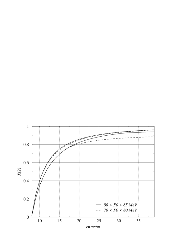
Figure 2: $X(2)$ as a function of $r$ for several values of $F_{0}$

Therefore, $X(2)$ does not reach its maximum for the paramagnetic bound $X(2)=X(3)|_{\mathrm{max}}$, whereas its minimum is the smallest of the two values obtained for $X(3)=0$ and $X(3)=X(3)|_{\mathrm{max}}$. The dependence on $r$ of the minimal value of $X(2)$ can be guessed rather easily. For large $r$, the term linear in $X(3)$ in Eq. (2.2) can be neglected: the minimum of $X(2)$ occurs for $X(3)=X(3)|_{\mathrm{max}}$. For small $r$, $X(2)$ and $X(3)$ tend to 0, and the term quadratic in $X(3)$ should be small with respect to the linear term. Therefore, $X(2)$ reaches its minimum for $X(3)=0$ when $r$ is small.

The numerical analysis of Eq. (2.2), including $\Delta Z^{S}$, supports this intuitive description. In Fig. 2, the variation ranges of $X(2)$ are plotted for several values of $F_{0}$. The curve for the minimum of $X(2)$ exhibits a cusp when the minimum of $X(2)$ corresponds no more to $X(3)=0$, but to $X(3)|_{\mathrm{max}}$. $X(2)$ appears to be strongly correlated to $r$, even though a large value of $X(2)\sim 0.9$ can be associated to a broad range of $r$.

3 Constraints from the pseudoscalar decay constants

3.1 Role of $L_{4}$

The decomposition used for the Goldstone boson masses can be adapted to the decay constants:

$$F_{\pi}^{2} = F_{0}^{2}+2m\xi+2(2m+m_{s})\tilde{\xi}$$

$$\quad+\frac{1}{16\pi^{2}}\frac{F_{\pi}^{2}M_{\pi}^{2}}{F_{0}^{2}}X(3)\left[2\log\frac{M_{K}^{2}}{M_{\pi}^{2}}+\log\frac{M_{\eta}^{2}}{M_{K}^{2}}\right]+\varepsilon_{\pi},$$

$$F_{K}^{2} = F_{0}^{2}+(m+m_{s})\xi+2(2m+m_{s})\tilde{\xi}+\frac{1}{2}\frac{F_{\pi}^{2}M_{\pi}^{2}}{F_{0}^{2}}X(3)L+\varepsilon_{K},$$ (25)

with the scale-independent constants related to $L_{4}$ and $L_{5}$:

$$\xi = 8B_{0}\left[L_{5}(\mu)-\frac{1}{256\pi^{2}}\left(\log\frac{M_{K}^{2}}{\mu^{2}}+2\log\frac{M_{\eta}^{2}}{\mu^{2}}\right)\right],$$ (26)

$$\tilde{\xi} = 8B_{0}\left[L_{4}(\mu)-\frac{1}{256\pi^{2}}\log\frac{M_{K}^{2}}{\mu^{2}}\right],$$ (27)

Eqs. (3.1) and (25) contain all the terms constant or linear in quark masses in the expansion of $F_{\pi}^{2}$ and $F_{K}^{2}$, whereas $\varepsilon_{P}$ denote remainders of order $O(m_{\mathrm{quark}}^{2})$. There is also a formula for $F_{\eta}$, which can be written as:

$$F_{\eta}^{2} = \frac{4}{3}F_{K}^{2}-\frac{1}{3}F_{\pi}^{2}+\frac{1}{24\pi^{2}}\frac{M_{\pi}^{2}F_{\pi}^{2}}{F_{0}^{2}}rX(3)\log\frac{M_{\eta}^{2}}{M_{K}^{2}}$$

$$\qquad+\frac{1}{48\pi^{2}}\frac{M_{\pi}^{2}F_{\pi}^{2}}{F_{0}^{2}}X(3)\left(\log\frac{M_{\eta}^{2}}{M_{K}^{2}}-\log\frac{M_{K}^{2}}{M_{\pi}^{2}}\right)+\varepsilon_{\eta}-\frac{4}{3}\varepsilon_{K}+\frac{1}{3}\varepsilon_{\pi}.$$

The two scale-independent constants can be extracted from Eqs. (3.1) and (25):

$$\frac{2m\xi}{F_{\pi}^{2}} = \tilde{\eta}(r)+\frac{1}{32\pi^{2}}\frac{F_{\pi}^{2}}{F_{0}^{2}}\frac{M_{\pi}^{2}}{F_{\pi}^{2}}\frac{X(3)}{r-1}\left[5\log\frac{M_{K}^{2}}{M_{\pi}^{2}}+3\log\frac{M_{\eta}^{2}}{M_{K}^{2}}\right],$$

$$+\frac{2}{r-1}\left[\frac{\varepsilon_{\pi}}{F_{\pi}^{2}}-\frac{\varepsilon_{K}}{F_{\pi}^{2}}\right]$$

$$\frac{2m\tilde{\xi}}{F_{\pi}^{2}} = \frac{1}{r+2}\left\{1-\tilde{\eta}(r)-\frac{F_{0}^{2}}{F_{\pi}^{2}}\right.$$

$$\qquad\left.-\frac{1}{32\pi^{2}}\frac{F_{\pi}^{2}}{F_{0}^{2}}\frac{M_{\pi}^{2}}{F_{\pi}^{2}}X(3)\left[\frac{4r+1}{r-1}\log\frac{M_{K}^{2}}{M_{\pi}^{2}}+\frac{2r+1}{r-1}\log\frac{M_{\eta}^{2}}{M_{K}^{2}}\right]\right\}$$

$$+\frac{1}{r+2}\left[\frac{2}{r-1}\frac{\varepsilon_{K}}{F_{\pi}^{2}}-\frac{r+1}{r-1}\frac{\varepsilon_{\pi}}{F_{\pi}^{2}}\right],$$

with:

$$\tilde{\eta}(r)=\frac{2}{r-1}\left(\frac{F_{K}^{2}}{F_{\pi}^{2}}-1\right)\sim\frac{0.977}{r-1},$$ (31)

where the latter estimate is obtained for $F_{K}/F_{\pi}=1.22$.

$\xi$ (i.e. $L_{5}$) turns out to depend essentially on $X(3)$ and $r$, whereas $\tilde{\xi}$ (i.e. $L_{4}$) is related to the difference between $F(3)$ and $F_{\pi}$. Eq. (3.1) leads to a quadratic equation for $[F(3)/F_{\pi}]^{2}$, involving $L_{4}$:

$$\left(\frac{F(3)}{F_{\pi}}\right)^{4}-(1-\tilde{\eta}-\varepsilon)\left(\frac{F(3)}{F_{\pi}}\right)^{2}+\lambda X(3)=0,$$ (32)

with:

$$\lambda = 8(r+2)\frac{M_{\pi}^{2}}{F_{\pi}^{2}}\left\{L_{4}(\mu)-\frac{1}{256\pi^{2}}\log\frac{M_{K}^{2}}{\mu^{2}}\right.$$

$$\left.+\frac{1}{256\pi^{2}}\frac{1}{(r+2)(r-1)}\left[(4r+1)\log\frac{M_{K}^{2}}{M_{\pi}^{2}}+(2r+1)\log\frac{M_{\eta}^{2}}{M_{K}^{2}}\right]\right\},$$

$$\varepsilon = \frac{r+1}{r-1}\frac{\varepsilon_{\pi}}{F_{\pi}^{2}}-\left(\tilde{\eta}+\frac{2}{r-1}\right)\frac{\varepsilon_{K}}{F_{K}^{2}}.$$ (34)

Eq. (32) has the solution:

$$\left(\frac{F(3)}{F_{\pi}}\right)^{2}=\frac{1-\tilde{\eta}-\varepsilon+\sqrt{\left(1-\tilde{\eta}-\varepsilon\right)^{2}-4\lambda X(3)}}{2}.$$ (35)

Notice that this formula is very close to Eq. (14), that relates $X(3)$ to $L_{6}(\mu)$ through the parameter $\kappa$. For $r=25$, the factor in front of the curly brackets in the definition of $\lambda$ is of order $460$, and $\lambda$ vanishes for $L_{4}(M_{\rho})=-0.51\cdot 10^{-3}$.

Figure 3: $F(2)$ (crosses) and $F(3)$ (no symbol) as functions of $L_{4}(M_{\rho})\cdot 10^{3}$ and $r=m_{s}/m$ (solid lines: $r=20$, dashed lines: $r=25$, dotted lines: $r=30$) for $X(3)$=0.9 (upper plot) and 0.5 (lower plot).

Eq. (32) admits a solution only if $\lambda X(3)\leq(1-\tilde{\eta}-\varepsilon)^{2}/4$. From Eq. (35), we get then a range for $F(3)$:

$$\frac{1-\tilde{\eta}-\varepsilon}{2}\leq\left(\frac{F(3)}{F_{\pi}}\right)^{2}\leq 1-\tilde{\eta}-\varepsilon.$$ (36)

The variations of $F(3)$ with $L_{4}(M_{\rho})$ are plotted for three values of $r$ and $X(3)=0.9$ and 0.5 in Fig. 3. When $X(3)$ decreases, the allowed range for $L_{4}$ broadens. This is due to the definition of $L_{4}$, which relates $B_{0}L_{4}=\Sigma(3)L_{4}/F^{2}(3)$ to the low-energy behavior of a QCD Green function. $[F(3)/F_{\pi}]^{2}$ starts at 0.9 (for the lowest possible value of $L_{4}(M_{\rho})$) and decreases until 0.5. $F(3)$ can thus vary from 87 to 65 MeV, depending on the value of $L_{4}(M_{\rho})$.

3.2 Paramagnetic inequality for $F^{2}$

We obtain $F(2)$ by taking the limit:

$$F^{2}(2)=\lim_{m\to 0}F_{\pi}^{2}=F(3)^{2}+2m_{s}\tilde{\xi}|_{m=0}+\varepsilon_{2},$$ (37)

keeping $m_{s}$ fixed. We have $\varepsilon_{2}=\lim_{m\to 0}\varepsilon_{\pi}$ and $\tilde{\xi}|_{m=0}=\tilde{\xi}+B_{0}\Delta\tilde{\xi}$, with

$$\Delta\tilde{\xi}=\frac{1}{32\pi^{2}}\log\frac{M_{K}^{2}}{\bar{M}_{K}^{2}}.$$ (38)

$\Delta\tilde{\xi}$ has a tiny effect on the results, similarly to $\Delta Z^{S}$ for $X(3)$. We get the equation:

$$\left[\frac{F(2)}{F_{\pi}}\right]^{2}=\frac{r}{r+2}\left\{[1-\tilde{\eta}]+\frac{2}{r}\left[\frac{F(3)}{F_{\pi}}\right]^{2}-X(3)\phi\left[\frac{F_{\pi}}{F(3)}\right]^{2}-\varepsilon_{F}\right\},$$ (39)

with:

$$\varepsilon_{F} = \frac{r+1}{r-1}\frac{\varepsilon_{\pi}}{F_{\pi}^{2}}-\frac{r+2}{r}\frac{\varepsilon_{2}}{F_{\pi}^{2}}-\left(\tilde{\eta}+\frac{2}{r-1}\right)\frac{\varepsilon_{K}}{F_{K}^{2}}$$ (40)

$$= \frac{1}{F_{\pi}^{2}}\left[\frac{r+1}{r-1}\varepsilon_{\pi}-\frac{r+2}{r}\lim_{m\to 0}\varepsilon_{\pi}\right]-\left(\tilde{\eta}+\frac{2}{r-1}\right)\frac{\varepsilon_{K}}{F_{K}^{2}},$$ (41)

$$\phi = \frac{1}{32\pi^{2}}\frac{M_{\pi}^{2}}{F_{\pi}^{2}}\left[\frac{4r+1}{r-1}\log\frac{M_{K}^{2}}{M_{\pi}^{2}}+\frac{2r+1}{r-1}\log\frac{M_{\eta}^{2}}{M_{K}^{2}}+(r+2)\log\frac{\bar{M}_{K}^{2}}{M_{K}^{2}}\right].$$ (42)

It is interesting to compare the expression of $F(2)$ as a function of $F(3)$ with Eq. (2.2) that relates $X(2)$ to $X(3)$. Even though the equations look rather similar, we can notice that Eq. (2.2) is a quadratic function of $X(3)$ whereas Eq. (39) involves $[F(3)/F_{\pi}]^{2}$ and its inverse $[F_{\pi}/F(3)]^{2}$. Moreover, Eq. (39) is an increasing function of $F(3)$, whereas $X(2)$ is not monotonous with $X(3)$. On the other hand, $\varepsilon_{F}$ suppresses the remainders $\varepsilon_{P}/F_{P}^{2}$ by a factor $m/m_{s}$, in a comparable way to $\delta_{X}$.

The paramagnetic inequality $F(2)\geq F(3)$ is translated into an upper bound for $F(3)$:

$$\left(\frac{F(3)}{F_{\pi}}\right)^{2}\leq\frac{1-\tilde{\eta}-\varepsilon_{F}+\sqrt{\left(1-\tilde{\eta}-\varepsilon_{F}\right)^{2}-4\phi X(3)}}{2}.$$ (43)

A quick estimate shows that the condition $X(3)\leq(1-\tilde{\eta}-\varepsilon_{F})^{2}/(4\phi)$ is satisfied for any $r$ between $\tilde{r}_{1}$ and $\tilde{r}_{2}$. This paramagnetic bound corresponds to a lower bound for $L_{4}(\mu)$:

$$L_{4}(\mu)>\frac{1}{256\pi^{2}}\log\frac{\bar{M}_{K}^{2}}{\mu^{2}}.$$ (44)

The term $\log(\bar{M}_{K}^{2})$ is very weakly dependent on $r$, $X(3)$ and $F(3)$. If we scan the acceptable range of variation for these three parameters, we obrain the lower bound $L_{4}(M_{\rho})>-0.37\cdot 10^{-3}$. We notice that the curves for $F(2)$ and $F(3)$ cross each other at this value in Fig. 3.

Since $\phi>0$, Eqs. (36) and (43) lead to the range:

$$\frac{1-\tilde{\eta}-\varepsilon}{2}\leq\frac{F(3)^{2}}{F_{\pi}^{2}}\leq 1-\tilde{\eta}-\mathrm{max}(\varepsilon_{F},\varepsilon).$$ (45)

The bounds on $F(3)$ are indicated in Tab. 1 (neglecting the remainders $\varepsilon$ and $\varepsilon_{F}$). Table 1 collects for several values of $r$ the corresponding bounds for $F(2)$, obtained using Eq. (39). It gives also the values of $X(3)$ and $F(3)$ that saturate both paramagnetic bounds: $F(2)=F(3)$ and $X(2)=X(3)$. In this case, the Zweig rule would be violated neither for the masses nor for the decay constants.

	$F(3)$ [MeV]				$F(2)$ [MeV]				No ZR violation
r	min		max		min		max		$F$ [MeV]		$X$
10	61.	69	87.	24	81.	31	87.	24	85.	57	0.	403
15	63.	02	89.	12	82.	34	89.	12	86.	17	0.	751
20	63.	63	89.	99	83.	02	89.	99	86.	71	0.	860
25	63.	99	90.	50	83.	38	90.	50	87.	08	0.	905
30	64.	23	90.	83	83.	43	90.	83	87.	35	0.	928
35	64.	39	91.	06	83.	14	91.	06	87.	55	0.	940

Table 1: On the left hand-side, bounds for $F(3)$. In the middle, corresponding bounds for $F(2)$. On the right hand-side, values of $F(3)$ and $X(3)$ saturating both paramagnetic inequalities: $F(2)=F(3)$ and $X(2)=X(3)$.

		$r=20$								$r=25$								$r=30$
$L_{6}$		4		5		7		8		4		5		7		8		4		5		7		8
-0.	2	-0.	284	2.	410	-1.	259	2.	624	-0.	282	1.	603	-0.	503	0.	994	-0.	284	1.	130	-0.	185	0.	298
-0.	1	-0.	264	2.	628	-1.	452	3.	044	-0.	261	1.	812	-0.	604	1.	224	-0.	262	1.	332	-0.	233	0.	416
0.		-0.	246	2.	824	-1.	636	3.	445	-0.	242	1.	993	-0.	699	1.	440	-0.	243	1.	501	-0.	276	0.	525
0.	2	-0.	215	3.	167	-1.	986	4.	207	-0.	210	2.	306	-0.	880	1.	848	-0.	211	1.	790	-0.	360	0.	730
0.	4	-0.	188	3.	466	-2.	318	4.	930	-0.	184	2.	572	-1.	050	2.	232	-0.	184	2.	036	-0.	439	0.	925
1.		-0.	121	4.	209	-3.	256	6.	966	-0.	116	3.	228	-1.	532	3.	314	-0.	117	2.	631	-0.	664	1.	471
-0.	2	0.	068	1.	833	-0.	816	1.	653	-0.	013	1.	174	-0.	325	0.	586	-0.	065	0.	782	-0.	117	0.	124
-0.	1	0.	133	2.	088	-0.	999	2.	056	0.	053	1.	414	-0.	420	0.	804	0.	002	1.	014	-0.	161	0.	236
0.		0.	190	2.	310	-1.	176	2.	442	0.	108	1.	616	-0.	509	1.	008	0.	055	1.	203	-0.	202	0.	340
0.	2	0.	287	2.	684	-1.	503	3.	156	0.	200	1.	953	-0.	678	1.	391	0.	144	1.	513	-0.	290	0.	533
0.	4	0.	368	3.	002	-1.	814	3.	833	0.	277	2.	234	-0.	837	1.	751	0.	217	1.	770	-0.	354	0.	715
1.		0.	567	3.	781	-2.	696	5.	751	0.	463	2.	915	-1.	291	2.	774	0.	392	2.	384	-0.	565	1.	232

Table 2: Low-energy constants $L_{i}(M_{\rho})\cdot 10^{3}$ as functions of $L_{6}(M_{\rho})\cdot 10^{3}$ and $r=m_{s}/m$, for $F_{0}$=85 MeV (upper part) and 75 MeV (lower part).

4 Sensitivity of low-energy constants to ZR violation

The equations (16), (17), (3.1) and (3.1) can be used to extract the LEC’s $L_{i=4,5,7,8}$ as functions of $r$, $F_{0}$ et $X(3)$, or equivalently, of $L_{6}$, $F_{0}\equiv F(3)$ and $r$ using Eq. (14). Results are shown in Tab. 2 as a function of $L_{6}$, for 2 values of $F_{0}$ and 3 values of $r$.

This table has been obtained by neglecting the higher-order terms $\delta_{P}$ and $\epsilon_{P}$, which start at the next-to-next-to-leading order (NNLO). If the size of these remainders is large, the values collected in these tables should be clearly modified. If we keep considering the low-energy constants as functions of $L_{6}(M_{\rho})$ and we change the relative size of the NNLO remainders within a range of 5%, the corresponding variations of $X(3)$ are of order $\pm 0.02$. The impact on the other LEC’s is larger for smaller $X(3)$ (of order $\pm 0.3\cdot 10^{-3}$ for $X(3)\sim 0.8$, $r\sim 25$).

The authors of Ref. [6] have estimated the NNLO remainders in the Standard Framework. The authors assume first $L_{4}(M_{\rho})=L_{6}(M_{\rho})=0$ and $r=24$, estimate $O(p^{6})$ counterterms (Standard counting) through a saturation of the associated correlators by resonances, and fit globally on the available data (masses, decay constants, form factors). For the decay constants, the obtained NNLO remainders $\epsilon_{P}$ are less than 5%. The situation is less clear for the masses, due to a bad convergence of the series. For instance, Ref. [6] has obtained the decomposition: $M^{2}_{\pi}/(M^{2}_{\pi})_{\mathrm{phys}}=0.746+0.007+0.247$, where the three terms correspond respectively to the leading $O(m)$, next-to-leading $O(m^{2})$ and next-to-next-to-leading $O(m^{3})$ orders. Ref. [6] suggested that a variation of $L_{4}(M_{\rho})$ and $L_{6}(M_{\rho})$ could make the NNLO contribution decrease, but a competition occurs then between the $O(m^{2})$ term and the leading-order term.

Such a competition could be understood from our analysis as a consequence of the suppression of the three-flavor condensate $X(3)$. It would be of great interest to proceed to the same analysis as in Ref. [6], and to allow a competition between the terms linear and quadratic in quark masses. This might improve the convergence of the expansion of Goldstone boson observables in powers of quark masses. Even if the three-flavor condensate $X(3)$ is suppressed (first term of the series for pseudoscalar masses), we expect a global convergence of the series, i.e. small higher-order remainders $\delta_{P}$ and $\epsilon_{P}$.

Standard values of the LEC’s at order $O(p^{4})$ can be found in Ref. [3], and were derived with the supposition that the ZR violating LEC’s $L_{6}(\mu)$ and $L_{4}(\mu)$ were suppressed at the scale $\mu=M_{\eta}$. The following values have been obtained: $L_{4}(M_{\rho})\cdot 10^{3}=-0.3\pm 0.5$, $L_{5}(M_{\rho})\cdot 10^{3}=1.4\pm 0.5$, $L_{6}(M_{\rho})\cdot 10^{3}=-0.2\pm 0.3$, $L_{7}(M_{\rho})\cdot 10^{3}=-0.4\pm 0.2$, $L_{8}(M_{\rho})\cdot 10^{3}=0.9\pm 0.3$. These values are compatible with our analysis: it can be seen on the first lines of Table 2, with $L_{6}(M_{\rho})\sim-0.2\cdot 10^{-3}$, $X(2)\sim X(3)\sim 0.9$, $r=25$, $F_{0}=85$ MeV. The values of $L_{4}(M_{\rho})$ and $L_{6}(M_{\rho})$ correspond also to the lower bounds derived from the saturation of the paramagnetic inequalities for $F^{2}$ and $X$: $X(2)=X(3)$ and $F(2)=F(3)$.

We see that $L_{4}$ is weakly sensitive to $L_{6}$, in agreement with Eqs. (27) and (3.1). For large $r$, and $F_{0}$ close to $F_{\pi}$, $1-\tilde{\eta}(r)-F_{0}^{2}/F_{\pi}^{2}$ is nearly vanishing, so that $L_{4}$ is mainly fixed by the last term in Eq. (3.1) with no dependence on $X(3)$. On the contrary, $L_{5}$ is clearly dependent on the value of $L_{6}$. We can look at Eq. (3.1) to understand this phenomenon : $\tilde{\eta}(r)$ may be small, but it never vanishes. The first term in Eq. (3.1) leads therefore to large values of $L_{5}$ when $X(3)$ decreases, whatever values we choose for $r$ and $F_{0}$ (this is related to the definition of $L_{5}$). The Gell-Mann–Okubo formula Eq. (17) correlates strongly $L_{7}$ and $L_{8}$, leading to $L_{7}\simeq-L_{8}/2$.

From this analysis of the pseudoscalar masses and decay constants, we cannot conclude whether $\bar{q}q$ fluctuations have important effects on the chiral structure of QCD vacuum. However, the values of LEC’s are extremely sensitive to the value of $L_{6}(M_{\rho})$. A small shift of $L_{6}$ towards positive values would immediately split $X(2)$ and $X(3)$, and increase strongly $L_{8}(M_{\rho})$ and $L_{5}(M_{\rho})$. We will now use additional information from experimental data in the scalar sector, in order to constrain $L_{6}(M_{\rho})$.

5 Sum rule for $X(2)-X(3)$

5.1 Correlator of two scalar densities

We introduce the correlator [17, 18]:

$$\Pi(p^{2})=i\frac{mm_{s}}{M^{2}_{\pi}M^{2}_{K}}\lim_{m\to 0}\int d^{4}x\ e^{ip\cdot x}\ \langle 0|T\{\bar{u}u(x)\ \bar{s}s(0)\}|0\rangle,$$ (46)

that is invariant under the QCD renormalization group, and violates the Zweig rule in the $0^{++}$ channel. For $m_{s}\neq 0$, $\Pi$ is a $\mathrm{SU}_{L}(2)\otimes\mathrm{SU}_{R}(2)$ order parameter, related to the derivative of $\Sigma(2)$ with respect to $m_{s}$: $mm_{s}\partial\Sigma(2)/\partial m_{s}=M_{\pi}^{2}M_{K}^{2}\Pi(0)$.

We can use the relation Eq. (2.2) between $r$, $X(3)$ and $X(2)$ to compute $\partial\Sigma(2)/\partial m_{s}$. Eq. (5) can be used to compute $(\partial Z^{S}/\partial m_{s})_{m=0}$. This leads to an equation involving $Z^{S}$ and $\Pi(0)$:

$$X(2)-X(3) = \frac{2mm_{s}}{F_{\pi}^{2}M_{\pi}^{2}}\left.Z^{S}\right|_{m=0}+\frac{m}{F_{\pi}^{2}M_{\pi}^{2}}\lim_{m\to 0}\frac{F_{\pi}^{2}\delta_{\pi}}{m}$$ (48)

$$= \frac{2M_{K}^{2}}{F_{\pi}^{2}}\Pi(0)+\frac{r[X(3)]^{2}}{32\pi^{2}}\frac{F_{\pi}^{2}M_{\pi}^{2}}{F_{0}^{4}}\left(\bar{\lambda}_{K}+\frac{2}{9}\bar{\lambda}_{\eta}\right)$$

$$\qquad+\frac{m}{F_{\pi}^{2}M_{\pi}^{2}}\left(1-m_{s}\frac{\partial}{\partial m_{s}}\right)\lim_{m\to 0}\frac{F_{\pi}^{2}\delta_{\pi}}{m},$$

with the logarithmic derivatives: $\bar{\lambda}_{P}=m_{s}\cdot\partial(\log\bar{M}_{P}^{2})/\partial m_{s}$. This equation contains the NNLO remainder $F_{\pi}^{2}\delta_{\pi}$ in the quark mass expansion of $F_{\pi}^{2}M_{\pi}^{2}$. Its leading term is $O(mm_{s}^{2})$, so that the last term in Eq. (48) should be of order $\sim(-\delta_{\pi}/M_{\pi}^{2})$.

$L_{6}$ (or the difference $X(2)-X(3)$) measures the violation of the Zweig rule in the scalar channel. We are going to exploit experimental information about this violation and to evaluate $\Pi(0)$ through the sum rule:

$$\Pi(0) = \frac{1}{\pi}\int_{0}^{s_{1}}ds\ \mathrm{Im}\ \Pi(s)\ \frac{1}{s}\left(1-\frac{s}{s_{0}}\right)$$

$$\qquad+\frac{1}{\pi}\int_{s_{1}}^{s_{0}}ds\ \mathrm{Im}\ \Pi(s)\ \frac{1}{s}\left(1-\frac{s}{s_{0}}\right)+\frac{1}{2i\pi}\int_{|s|=s_{0}}ds\ \Pi(s)\ \frac{1}{s}\left(1-\frac{s}{s_{0}}\right).$$

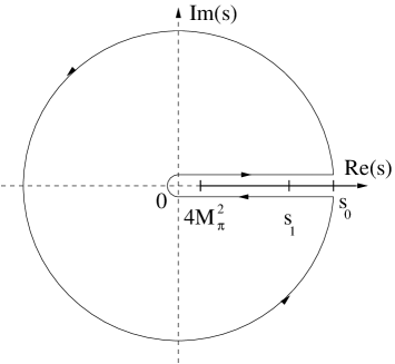
Figure 4: Contour of the integral in the sum rule for the correlator $\langle\bar{u}u\ \bar{s}s\rangle$.

The three terms will be estimated in different ways:

• For $0\leq\sqrt{s}\leq\sqrt{s_{1}}\sim 1.2\ \mathrm{GeV}$, the spectral function $\mathrm{Im}\ \Pi$ is obtained by solving Omnès-Muskhelishvili equations for two coupled channels, using several $T$-matrix models in the scalar sector.

• For $\sqrt{s_{1}}\leq\sqrt{s}\leq\sqrt{s_{0}}\sim 1.5\ \mathrm{GeV}$, the spectral function under $s_{1}$ is exploited through another sum rule in order to bound the contribution of the integral.

• For $|s|=s_{0}$, we estimate the integral through Operator Product Expansion (OPE).

5.2 Asymptotic behavior

$\Pi$ can be expanded using OPE:

$$\Pi(p^{2}) = i\frac{mm_{s}}{M^{2}_{\pi}M^{2}_{K}}\lim_{m\to 0}\int d^{4}x\ e^{ip\cdot x}\ \langle 0|T[\bar{u}u(x)\ \bar{s}s(0)]|0\rangle$$ (50)

$${\displaystyle\mathop{\sim}_{P^{2}\to\infty}} \frac{mm_{s}}{M^{2}_{\pi}M^{2}_{K}}\sum_{n\geq 4}\frac{1}{(P^{2})^{n/2-1}}C^{(n)}(t)\langle 0|\mathcal{O}_{n}|0\rangle,$$ (51)

with $P^{2}=-p^{2}$, $\mu$ a renormalization scale, $t=\mu^{2}/P^{2}$, and $\mathcal{O}_{n}$ a combination of $n$-dimensional operators. $\Pi$ transforms chirally as $(\bar{u}u)(\bar{s}s)$ and we take the chiral limit $m\to 0$. Hence, the lowest-dimension operator is $\mathcal{O}_{4}=m_{s}\bar{u}u$, and the contributing diagrams include at least two gluonic lines [17].

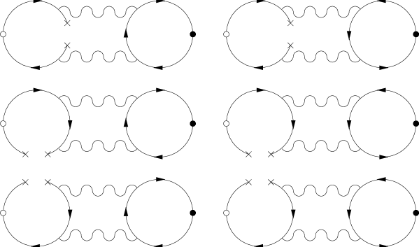
Figure 5: Feynman diagrams contributing to $m_{s}\langle\bar{u}{u}\rangle$ in OPE of $\Pi$ (lowest order in $\alpha_{s}$). The white circle is the scalar source $\bar{u}u$, the black one $\bar{s}s$.

We will work in dimensional regularization ($d=4-2\omega$). In the class of t’Hooft’s gauges, the gluon propagator reads:

$$\frac{-i}{k^{2}+i\epsilon}\left(g_{\mu\nu}-(1-\xi)\frac{k_{\mu}k_{\nu}}{k^{2}+i\epsilon}\right)\delta_{ab},$$ (52)

with $\xi$ a free real parameter. The Wilson coefficient of $m_{s}\bar{u}u$ (at the leading order) is obtained by adding 6 two-loop integrals. It is easy to see that the contributions of $\xi$ and $\xi^{2}$ cancel in this sum of integrals. Hence, we check that the Wilson coefficient of $m_{s}\bar{u}u$ at the leading order is independent of the chosen gauge, in the classe of t’Hooft’s gauges.

We want the large-$P^{2}$ limit of integrals like:

$$g_{s}^{4}\mu^{4\omega}m_{s}\langle\bar{u}u\rangle\frac{1}{p^{2}}\int\frac{d^{4}q}{(2\pi)^{d}}\frac{d^{4}k}{(2\pi)^{d}}\mathcal{P}(p^{2},q^{2},k^{2},p\cdot q,p\cdot k,q\cdot k,m_{s}^{2})$$ (53)

$$\qquad\times\frac{1}{[(p-q)^{2}-m_{0}^{2}]^{n_{2}}[q^{2}-m_{0}^{2}]^{n_{3}}}$$

$$\qquad\times\frac{1}{[(k+p)^{2}-m_{s}^{2}]^{n_{4}}[(k+q)^{2}-m_{s}^{2}]^{n_{5}}[k^{2}-m_{s}^{2}]^{n_{6}}},$$

where $\mathcal{P}$ is a polynomial of degree 2. $m_{0}$ corresponds at the same time to $m=m_{u}=m_{d}$ for fermion propagators in the loop of $u-d$ quarks, and to a fictitious mass to regularize infrared gluonic divergences (we take at the end the limit $m_{0}\to 0$).

Using identities like $2(k\cdot q)=[(k+q)^{2}+m_{s}^{2}]-[k^{2}+m_{s}^{2}]-q^{2}$, we can reexpress the sum in terms of:

$$\frac{1}{p^{2\nu_{0}}}J(\{\nu_{i}\},\{m_{i}\},p)=\frac{1}{p^{2\nu_{0}}}\int\frac{d^{4}q\ d^{4}k}{[q^{2}-m_{0}^{2}]^{\nu_{1}}[k^{2}-m_{s}^{2}]^{\nu_{2}}}$$ (54)

$$\qquad\times\frac{1}{[(k+q)^{2}-m_{s}^{2}]^{\nu_{3}}[(p-q)^{2}-m_{0}^{2}]^{\nu_{4}}[(k+p)^{2}-m_{s}^{2}]^{\nu_{5}}},$$

with $m_{1}=m_{4}=m_{0}$ and $m_{2}=m_{3}=m_{5}=m_{s}$. These integrals are formally identical to the ones arising for two-loop self-energies. The behavior of such integrals at large external momentum has already been studied. The basic idea consists in following the flux of the large external momentum through the Feynman diagrams, in order to Taylor expand the propagators [24]. This procedure, based on the asymptotic expansion theorem [25], is sketched in App. B.

Rather lengthy computations lead to the first term arising in the OPE of the correlator. Some integrals contain poles in $1/\omega$, but these divergences cancel when all the contributions are summed (this cancellation is a non-trivial check of the procedure). The first term in OPE is:

$$i\frac{mm_{s}}{M_{\pi}^{2}M_{K}^{2}}\lim_{m\to 0}\int d^{4}x\ e^{ip\cdot x}\ \langle 0|T\{m\bar{u}u(x)\ m_{s}\bar{s}s(0)\}|0\rangle$$ (55)

$$\quad{\displaystyle\mathop{\sim}_{P^{2}\to\infty}}-\frac{18[1-2\zeta(3)]}{P^{2}}\left(\frac{\alpha_{s}}{\pi}\right)^{2}\frac{m_{s}^{2}}{M_{\pi}^{2}M_{K}^{2}}m\langle\bar{u}u\rangle.$$

The involved condensate should be the two-flavor one ($m\to 0$, $m_{s}\neq 0$).

5.3 Contribution for $s\leq s_{1}$ : pion and kaon scalar form factors

5.3.1 Omnès-Muskhelishvili equations

In order to compute the integral:

$$\mathcal{I}=\frac{1}{\pi}\int_{0}^{s_{1}}ds\ \mathrm{Im}\ \Pi(s)\ \frac{1}{s}\left(1-\frac{s}{s_{0}}\right),$$ (56)

we have to know $\mathrm{Im}\ \Pi$ between 0 and $s_{1}$ ($\sqrt{s}_{1}\sim$ 1.2 Gev). The procedure is explained in detail in Refs. [17, 18], and we shall merely sketch its main features for completeness. In the range of energy between 0 and $s_{1}$, the $\pi\pi$- and $K\bar{K}$- channels should dominate the spectral function [17, 26, 27]. If we denote these channels respectively 1 and 2, the spectral function is:

$$\mathrm{Im}\ \Pi(s)=\frac{mm_{s}}{M^{2}_{\pi}M^{2}_{K}}\frac{1}{16\pi}\sum_{i=1,2}\sqrt{\frac{s-4M_{i}^{2}}{s}}[n_{i}F_{i}(s)][n_{i}G^{*}_{i}(s)]\theta(s-4M_{i}^{2}),$$ (57)

with the scalar form factors for the pion and the kaon:

$$\vec{F}(s)=\left(\begin{array}[]{c}\langle 0|\bar{u}u|\pi\pi\rangle\\ \langle 0|\bar{u}u|K\bar{K}\rangle\end{array}\right),\qquad\vec{G}(s)=\left(\begin{array}[]{c}\langle 0|\bar{s}s|\pi\pi\rangle\\ \langle 0|\bar{s}s|K\bar{K}\rangle\end{array}\right),$$ (58)

with $M_{1}=M_{\pi}$ and $M_{2}=M_{K}$. $n_{1}=\sqrt{3/2}$ and $n_{2}=\sqrt{2}$ are numerical factors related to the normalization of the states $|\pi\pi\rangle$ and $|K\bar{K}\rangle$.

The form factors are analytic functions in the complex plane, with the exception of a right cut along the real axis. They should have the asymptotic behaviour $F_{i}(s)\sim 1/s$ when $s\to\infty$, and verify a dispersion relation with no subtraction. Obviously, when $s$ increases, new channels open, and the two-channel approximation is no more sufficient. But we need $\vec{F}$ and $\vec{G}$ for $s\leq s_{1}$, and we are not interested in the behaviour of the spectral function at much higher energies. We can therefore suppose that the two-channel approximation is valid for any energies, with the discontinuity along the cut:

$$S_{ij} = \delta_{ij}+2i\sigma_{i}^{1/2}T_{ij}\sigma_{j}^{1/2}\theta(s-4M_{i}^{2})\theta(s-4M_{j}^{2}),$$ (59)

$$\mathrm{Im}\ F_{i}(s) = \sum_{j=1}^{n}T_{ij}^{*}(s)\sigma_{j}(s)F_{j}(s)\theta(s-4M_{j}^{2}),\ \sigma_{i}=\sqrt{\frac{s-4M_{i}^{2}}{s}},$$ (60)

and we will suppose in addition that the two-channel $T$-matrix model impose the correct asymptotic behaviour for $\vec{F}$ and $\vec{G}$.

Under these assumptions, $\vec{F}$ and $\vec{G}$ satisfy separately a set of coupled Omnès-Muskhelishvili equations [17, 26, 28, 29]:

$$F_{i}(s)=\frac{1}{\pi}\sum_{j=1}^{n}\int_{4M_{\pi}^{2}}^{\infty}ds^{\prime}\frac{1}{s^{\prime}-s}T_{ij}^{*}(s^{\prime})\sqrt{\frac{s^{\prime}-4M_{j}^{2}}{s^{\prime}}}\theta(s^{\prime}-4M_{j}^{2})F_{j}(s^{\prime}),$$ (61)

with the condition that the $T$ matrix leads to the expected decrease of the form factors for $s\to\infty$. Ref. [17] has proved a condition of existence and unicity for the solution of Eq. (61): $\Delta(\infty)-\Delta(4M_{\pi}^{2})=2\pi$, where $\Delta(s)$ is the sum of the $\pi\pi$ and $K\bar{K}$ phase shifts. In that case, the set of linear equations admits a unique solution, once the values at a given energy are fixed [18]. All the solutions are thus linear combinations of a basis, for instance the solutions $\vec{A}(s)$ and $\vec{B}(s)$ such as: $\vec{A}(0)={1\choose 0}$ and $\vec{B}(0)={0\choose 1}$. $\vec{F}$ and $\vec{G}$ can therefore be written as:

$$\vec{F}(s)=F_{1}(0)\vec{A}(s)+F_{2}(0)\vec{B}(s),\qquad\vec{G}(s)=G_{1}(0)\vec{A}(s)+G_{2}(0)\vec{B}(s).$$ (62)

The value of the form factors at zero is related to the derivatives of the pseudoscalar masses with respect to the quark masses:

$$F_{1}(0)=\frac{1}{2}\left(\frac{\partial M_{\pi}^{2}}{\partial m}\right)_{m=0}, F_{2}(0)=\frac{1}{2}\left(\frac{\partial M_{K}^{2}}{\partial m}\right)_{m=0},$$ (63)

$$G_{1}(0)=\left(\frac{\partial M_{\pi}^{2}}{\partial m_{s}}\right)_{m=0}=0, G_{2}(0)=\left(\frac{\partial M_{K}^{2}}{\partial m_{s}}\right)_{m=0}.$$ (64)

Up to now, we have followed the same line as Refs. [26, 17]. But in these papers, the value of the scalar form factors at zero was derived using Standard $\chi$PT, i.e. supposing that the three-flavor quark condensate dominates the expansion of the pseudoscalar masses. We are going to allow a competition between the terms linear and quadratic in quark masses, so that the normalization of the form factors may become rather different from what is considered in Refs. [17, 26]. In a similar way, the form factors that we will obtain could differ from the ones obtained by a matching with Standard one-loop expressions [27, 30].

We consider here three models of $T$-matrix, proposed respectively by Oller, Oset and Pelaez in Ref. [31], by Au, Morgan and Pennington in Ref. [32], and by Kaminski, Lesniak and Maillet in Ref. [33]. These models fit correctly the available data in the scalar sector under 1.3 Gev, as discussed in Refs. [17, 26, 31]. However, they have to be corrected for very low and very high energies, as discussed in Ref. [17]: chiral symmetry constrains the $\pi\pi$ phase shift near the threshold, and the asymptotic behavior of the phases shifts has to be changed to to insure existence and unicity for the solution of Eq. (61).

5.3.2 Contribution of the first integral

If we put Eq. (62) into Eq. (57), we obtain the spectral function as the sum of two contributions:

$$\mathrm{Im}\ \Pi(s) = \gamma_{\pi}\lambda_{K}\left[\frac{\sqrt{3}}{32\pi}\sum_{i=1,2}\sqrt{\frac{s-4M_{i}^{2}}{s}}A_{i}(s)B^{*}_{i}(s)\theta(s-4M_{i}^{2})\right]$$

$$+\gamma_{K}\lambda_{K}\frac{M_{K}^{2}}{M_{\pi}^{2}}\left[\frac{1}{16\pi}\sum_{i=1,2}\sqrt{\frac{s-4M_{i}^{2}}{s}}B_{i}(s)B^{*}_{i}(s)\theta(s-4M_{i}^{2})\right],$$

where the logarithmic derivatives of the masses are denoted:

$$\lambda_{P}=\frac{m_{s}}{M^{2}_{P}}\left(\frac{\partial M_{P}^{2}}{\partial m_{s}}\right)_{m=0}=\frac{m_{s}}{M^{2}_{P}}\frac{\partial\bar{M}_{P}^{2}}{\partial m_{s}},\qquad\gamma_{P}=\frac{m}{M^{2}_{P}}\left(\frac{\partial M_{P}^{2}}{\partial m}\right)_{m=0}.$$ (66)

The two bracketed functions in Eq. (5.3.2) can be plotted: the first one is called ”type $AB^{*}$”, the second one ”type $BB^{*}$”. It is also interesting to study how these two contributions cancel each other inside the spectral function, by taking the Standard tree-level estimates: $\gamma_{\pi}=1$, $\lambda_{K}=1-M_{\pi}^{2}/(2M_{K}^{2})$ and $\gamma_{K}=M_{\pi}^{2}/(2M_{K}^{2})$. A peak, corresponding to the narrow resonance $f_{0}(980)$ [8], arises with a height depending on the models: Ref. [31] leads to a smaller peak than Refs. [32] and [33].

Figure 6: Up: Contributions of type $BB^{*}$ (positive) and type $AB^{*}$ (negative) to the spectral function. Down: example of spectral function, obtained with $\gamma_{\pi}=1$, $\lambda_{K}=1-M_{\pi}^{2}/(2M_{K}^{2})$ and $\gamma_{K}=M_{\pi}^{2}/(2M_{K}^{2})$. In both cases, we plot the results for the $T$-matrix models of Ref. [31] (solid lines), Ref. [32] (dotted) and Ref. [33] (dashed).

The integral between 0 and $s_{1}$ in the sum rule Eq. (5.1) can be written, using Eq. (5.3.2):

$$\frac{1}{\pi}\int_{0}^{s_{1}}ds\ \mathrm{Im}\ \Pi(s)\ \frac{1}{s}\left(1-\frac{s}{s_{0}}\right)=\gamma_{\pi}\lambda_{K}\mathcal{I}_{AB}+\gamma_{K}\lambda_{K}\frac{M_{K}^{2}}{M_{\pi}^{2}}\mathcal{I}_{BB},$$ (67)

where $\mathcal{I}_{XY}=\mathcal{M}_{XY}^{(-1)}-\mathcal{M}_{XY}^{(0)}/s_{0}$, involves the moments:

$$\mathcal{M}^{(k)}_{AB} = \frac{\sqrt{3}}{32\pi^{2}}\int_{0}^{s_{1}}ds\ s^{k}\sum_{i=1,2}\sqrt{\frac{s-4M_{i}^{2}}{s}}A_{i}(s)B^{*}_{i}(s)\theta(s-4M_{i}^{2}),$$ (68)

$$\mathcal{M}^{(k)}_{BB} = \frac{1}{16\pi^{2}}\int_{0}^{s_{1}}ds\ s^{k}\sum_{i=1,2}\sqrt{\frac{s-4M_{i}^{2}}{s}}B_{i}(s)B^{*}_{i}(s)\theta(s-4M_{i}^{2}).$$ (69)

Notice that we solve Omnès-Muskhelishvili equations to obtain the scalar form factors of the pion and the kaon in the limit $m\to 0$ (and $m_{s}$ fixed at its physical value). But we consider $T$-matrix models fitting experimental data, with up and down quarks with their physical masses. The limit $m\to 0$ sets the $\pi\pi$-threshold to zero, changes $\pi\pi$ phase shifts near the threshold and shifts slightly the $K\bar{K}$ threshold. Such modifications should not alter significantly the general shape of the spectral function. In particular, the integral of the spectral function, dominated by the $f_{0}(980)$ peak, should be affected only marginally when $T_{\mathrm{m\neq 0}}$ is considered instead of $T_{\mathrm{m\to 0}}$.

5.4 Second sum rule : $s_{1}\leq s\leq s_{0}$

The contribution of the integral below $s_{1}$ is positive and dominated by the $f_{0}(980)$ peak. But according to Sec. 5.2, $\Pi$ is superconvergent, and the integral of the spectral function from 0 to infinity vanishes. $\mathrm{Im}\ \Pi(s)$ should therefore become negative in some range of energy. In particular, negative peaks should rather naturally appear in the spectral function, in relation with massive scalar resonances like $f_{0}(1370)$ and $f_{0}(1500)$ [8].

Let us suppose that the spectral function is negative for $s_{1}\leq s\leq s_{0}$. The contribution from the intermediate region in Eq. (48) can be estimated from:

$$\frac{1}{s_{0}}\mathcal{J}^{\prime}\leq-\frac{1}{\pi}\int_{s_{1}}^{s_{0}}ds\ \mathrm{Im}\ \Pi(s)\ \frac{1}{s}\left(1-\frac{s}{s_{0}}\right)\leq\frac{1}{s_{1}}\mathcal{J}^{\prime},$$ (71)

where $\mathcal{J}^{\prime}$ is the integral:

$$\mathcal{J}^{\prime}=\frac{1}{\pi}\int_{s_{1}}^{s_{0}}ds\ \mathrm{Im}\ \Pi(s)\ \left(1-\frac{s}{s_{0}}\right),$$ (72)

which satisfies the sum rule:

$$\frac{1}{\pi}\int_{0}^{s_{1}}ds\ \mathrm{Im}\ \Pi(s)\ \left(1-\frac{s}{s_{0}}\right)+\mathcal{J}^{\prime}+\frac{1}{2i\pi}\int_{|s|=s_{0}}\!\!\!ds\ \Pi(s)\ \left(1-\frac{s}{s_{0}}\right)=0$$ (73)

The first integral in Eq. (73) can be computed from the spectral function obtained in the previous section:

$$\frac{1}{\pi}\int_{0}^{s_{1}}ds\ \mathrm{Im}\ \Pi(s)\ \left(1-\frac{s}{s_{0}}\right)=\gamma_{\pi}\lambda_{K}\mathcal{I}^{\prime}_{AB}+\gamma_{K}\lambda_{K}\frac{M_{K}^{2}}{M_{\pi}^{2}}\mathcal{I}^{\prime}_{BB},$$ (74)

with $\mathcal{I}^{\prime}_{XY}=\mathcal{M}_{XY}^{(0)}-\mathcal{M}_{XY}^{(1)}/s_{0}$ involving the moments Eqs. (68)-(69).

The contribution from the complex circle [third integral in Eq. (73)] can be estimated through Operator Product Expansion (OPE), using the method described in the following section:

$$\frac{1}{2i\pi}\int_{|s|=s_{0}}\!\!\!ds\ \Pi(s)\ \left(1-\frac{s}{s_{0}}\right)$$ (75)

$$=9[1-2\zeta(3)]\frac{F_{\pi}^{2}}{M_{K}^{2}}X(2)m^{2}_{s}(s_{0})a^{2}(s_{0})$$

$$\quad\times\left\{1+\frac{\beta_{0}\gamma}{2}a(s_{0})+\left[\frac{\beta_{1}\gamma}{2}-\frac{\gamma(\gamma+1)}{8}\left(\frac{\pi^{2}}{3}-2\right)\beta_{0}^{2}\right]a^{2}(s_{0})\right\}+\ldots$$

$$=9[1-2\zeta(3)]\frac{F_{\pi}^{2}}{M_{K}^{2}}X(2)m^{2}_{s}(s_{0})a^{2}(s_{0})$$ (76)

$$\qquad\times[1+6.5\cdot a(s_{0})-25.125\cdot a^{2}(s_{0})].$$

5.5 High-energy contribution : $|s|=s_{0}$

We want the contribution of the integral on the large circle:

$$\mathcal{K}=\frac{1}{2i\pi}\!\!\int_{|s|=s_{0}}\!\!\!\!ds\ \Pi(s)\ \frac{1}{s}\left(1-\frac{s}{s_{0}}\right)=\frac{1}{2\pi}\int_{-\pi}^{\pi}d\theta\ (1+e^{i\theta})\ \Pi(p^{2}=-s_{0}e^{i\theta}).$$ (77)

The factor $(1-s/s_{0})$ suppresses the contribution stemming from the time-like region around $s_{0}$, so that we can use in this integral the Operator Product Expansion of $\Pi$ [34]. Once Renormalization Group Improvement is applied to Eq. (55), the QCD renormalization group invariant $m\langle\bar{u}u\rangle$ gets the coefficient:

$$a^{2}(P^{2})m_{s}^{2}(P^{2})=a^{2}(s_{0})m_{s}^{2}(s_{0})\times\left[\frac{a(P^{2})}{a(s_{0})}\right]^{8/b_{0}+2},$$ (78)

with $a(s)=\alpha_{s}(s)/\pi$ and $b_{0}=11-2N_{f}/3=9$. The integral Eq. (77) becomes:

$$\mathcal{K} = \frac{9[1-2\zeta(3)]}{2\pi}\frac{F_{\pi}^{2}}{M_{K}^{2}}X(2)\frac{m^{2}_{s}(s_{0})}{s_{0}}[a(s_{0})]^{-\frac{8}{b_{0}}}\int_{-\pi}^{\pi}ds\ (1+e^{-i\theta})\ a^{\gamma}(s_{0}e^{i\theta}),$$ (79)

with $\gamma=2+8/b_{0}=2+8/9$. To compute this integral, we expand $a(P^{2}=s_{0}e^{i\theta})$ in powers of $a(s_{0})$. The behaviour of $a(t)$ ($t$ complex) depends on the $\beta$ function:

$$t\frac{d}{dt}a(t)=\frac{1}{2\pi}\beta[a(t)], \frac{1}{\pi}\beta[a(t)]=-\beta_{0}a^{2}-\beta_{1}a^{3}+\ldots,$$ (80)

$$\beta_{0}=\frac{33-2N_{f}}{6}=\frac{9}{2}, \beta_{1}=\frac{306-38N_{f}}{24}=8.$$ (81)

The expansion of $a(s_{0}e^{i\theta})$ is:

$$a(s_{0}e^{i\theta})=a(s_{0})-\frac{i}{2}\beta_{0}\theta a^{2}(s_{0})+\left[\frac{i}{2}\beta_{1}\theta-\frac{1}{4}\theta\beta_{0}^{2}\theta^{2}\right]a^{3}(s_{0})+O(a^{4}).$$ (82)

We get:

$$\mathcal{K} = 9[1-2\zeta(3)]\frac{F_{\pi}^{2}}{M_{K}^{2}}X(2)\frac{m^{2}_{s}(s_{0})}{s_{0}}a^{2}(s_{0})$$

$$\quad\times\left\{1-\frac{\beta_{0}\gamma}{2}a(s_{0})-\left[\frac{\beta_{1}\gamma}{2}+\frac{\gamma(\gamma+1)}{8}\left(\frac{\pi^{2}}{3}-2\right)\beta_{0}^{2}\right]a^{2}(s_{0})\right\}+\ldots$$

$$= 9[1-2\zeta(3)]\frac{F_{\pi}^{2}}{M_{K}^{2}}X(2)\frac{m^{2}_{s}(s_{0})}{s_{0}}a^{2}(s_{0})[1-6.5\cdot a(s_{0})+48.236\cdot a^{2}(s_{0})].$$

This negative contribution is strongly suppressed by $\alpha^{2}_{s}$ and $m_{s}^{2}/s_{0}$. We have considered here $m_{s}\sim 200$ MeV, but the contribution of this integral is so small that the error due to $m_{s}$ and $\alpha_{s}$ can be neglected. Notice that duality is not supposed to arise in the scalar sector for as low energies as in other channels, due to a probably large contribution from the direct instantons in this sector [35].

6 Results

6.1 Logarithmic derivatives of pseudoscalar masses

The logarithmic derivatives of the masses are obtained from the expansions of $F_{P}^{2}$ and $F_{P}^{2}M_{P}^{2}$:

$$\lambda_{P}=\frac{m_{s}}{M^{2}_{P}}\left(\frac{\partial M_{P}^{2}}{\partial m_{s}}\right)_{m=0}=\frac{m_{s}}{M^{2}_{P}}\frac{\partial\bar{M}_{P}^{2}}{\partial m_{s}},\qquad\gamma_{P}=\frac{m}{M^{2}_{P}}\left(\frac{\partial M_{P}^{2}}{\partial m}\right)_{m=0}.$$ (84)

The corresponding expressions are given in App. C.1. We have $\lambda_{\pi}=0$ since it is proportional to the derivative of $M^{2}_{\pi}$ with respect to $m_{s}$ in the limit $m\to 0$.

		$r=20$						$r=25$						$r=30$
$X(3)$		$\gamma_{\pi}$		$\gamma_{K}$		$\gamma_{\eta}$		$\gamma_{\pi}$		$\gamma_{K}$		$\gamma_{\eta}$		$\gamma_{\pi}$		$\gamma_{K}$		$\gamma_{\eta}$
0.		0.	876	0.	090	0.	081	0.	930	0.	078	0.	068	0.	958	0.	070	0.	059
0.	3	0.	920	0.	082	0.	071	0.	970	0.	069	0.	058	0.	995	0.	060	0.	049
0.	5	0.	946	0.	074	0.	062	0.	992	0.	060	0.	048	1.	015	0.	051	0.	038
0.	7	0.	967	0.	064	0.	052	1.	009	0.	050	0.	036	1.	029	0.	039	0.	025
0.	8	0.	975	0.	059	0.	046	1.	016	0.	044	0.	030	1.	034	0.	033	0.	019
0.	9	-		-		-		1.	021	0.	038	0.	024	1.	038	0.	027	0.	013
0.		0.	892	0.	080	0.	072	0.	943	0.	070	0.	060	0.	970	0.	063	0.	053
0.	3	0.	941	0.	072	0.	062	0.	990	0.	061	0.	050	1.	011	0.	053	0.	041
0.	5	0.	965	0.	063	0.	051	1.	009	0.	051	0.	038	1.	029	0.	042	0.	029
0.	7	0.	980	0.	052	0.	039	1.	020	0.	038	0.	025	1.	037	0.	029	0.	015
0.	8	0.	983	0.	046	0.	032	1.	022	0.	032	0.	018	1.	037	0.	022	0.	009

Table 3: Logarithmic derivatives with respect to $m$ : $\gamma_{\pi}$, $\gamma_{K}$ and $\gamma_{\eta}$, as functions of $X(3)$ and $r$, for $F_{0}$=85 MeV (upper part) and $F_{0}$=75 MeV (lower part).

		$r=20$				$r=25$				$r=30$
$X(3)$		$\lambda_{K}$		$\lambda_{\eta}$		$\lambda_{K}$		$\lambda_{\eta}$		$\lambda_{K}$		$\lambda_{\eta}$
0.		1.	438	1.	398	1.	455	1.	416	1.	467	1.	428
0.	3	1.	391	1.	346	1.	383	1.	339	1.	366	1.	321
0.	5	1.	326	1.	276	1.	284	1.	231	1.	226	1.	169
0.	7	1.	236	1.	179	1.	148	1.	086	1.	041	0.	975
0.	8	1.	183	1.	123	1.	070	1.	005	0.	938	0.	871
0.	9	-		-		0.	986	0.	921	0.	833	0.	768
0.		1.	341	1.	310	1.	354	1.	323	1.	362	1.	332
0.	3	1.	302	1.	263	1.	287	1.	247	1.	261	1.	220
0.	5	1.	224	1.	177	1.	163	1.	111	1.	086	1.	029
0.	7	1.	109	1.	053	0.	991	0.	931	0.	858	0.	796
0.	8	1.	041	0.	982	0.	894	0.	834	0.	739	0.	681

Table 4: Logarithmic derivatives with respect to $m_{s}$ : $\lambda_{K}$ and $\lambda_{\eta}$, as functions of $r$ and $X(3)$, for $F_{0}$=85 MeV (upper part) and $F_{0}$=75 MeV (lower part).

We would obtain at the one-loop order in the Standard framework:

$$\gamma_{\pi}\sim 1,\qquad\gamma_{K}\sim\frac{M_{\pi}^{2}}{2M_{K}^{2}}=0.04,\qquad\gamma_{\eta}\sim\frac{M_{\pi}^{2}}{3M_{\eta}^{2}}=0.02,$$ (85)

$$\lambda_{K}\sim 1-\frac{M_{\pi}^{2}}{2M_{K}^{2}}=0.96,\qquad\lambda_{\eta}\sim\frac{4M_{K}^{2}}{3M_{\eta}^{2}}=1.09.$$ (86)

The logarithmic derivatives differ from these values because of the terms quadratic in the quark masses in the expansions of $F_{P}^{2}M_{P}^{2}$. The Tables 3-4 collect values of these derivatives for $r=20,25,30$, and $F_{0}$=75 MeV and 85 MeV. We note that the values for $F_{0}$=85 MeV, $r=25$, $X(3)\sim 0.8$ are in correct agreement with the Standard tree-level estimates Eqs. (85)-(86).

We can notice that $\gamma_{\pi}$ remains close to 1 if we change $F_{0}$, $r$ and $X(3)$. $\gamma_{\pi}$ involves the linear $m$-dependence of the pion mass, which can be written as: $F_{\pi}^{2}M_{\pi}^{2}=2m\Sigma(2)+O(m^{2})$. Therefore, $\gamma_{\pi}$ is related to the two-flavor quark condensate $\Sigma(2)$, which is very weakly dependent on the values of $F_{0}$ and $X(3)$ [it is affected by the value of $r$, but our tables show only large values of $r$ where $X(2)$ does not strongly vary]. On the other hand, $\gamma_{K}$ and $\gamma_{\eta}$ are rather sensitive to $X(3)$. These two logarithmic derivatives are $1/r$-suppressed when the three-flavor quark condensate is large. If $X(3)$ decreases, these 2 quantities feel strongly the presence of large higher-order contribution.

$\lambda_{K}$ and $\lambda_{\eta}$ increase from 1 to 1.4 when $X(3)$ decreases down to 0. If $X(3)$ vanishes, the pseudoscalar masses are dominated by terms quadratic in $m_{s}$. In that case, we would naively expect logarithmic derivatives to be twice as large as for $X(3)\sim 1$. To understand this discrepancy, it is useful to consider the second kind of logarithmic derivatives arising in Eq. (48):

$$\bar{\lambda}_{P}=\frac{m_{s}}{\bar{M}^{2}_{P}}\frac{\partial\bar{M}_{P}^{2}}{\partial m_{s}}=\frac{M_{P}^{2}}{\bar{M}^{2}_{P}}\lambda_{P},\qquad P=K,\eta$$ (87)

$\lambda_{P}$ and $\bar{\lambda}_{P}$ are related, but the first is suppressed with respect to the latter by a factor $\bar{M}^{2}_{P}/M_{P}^{2}$. For instance, in the limit of a vanishing three-flavor condensate, the expansion of $\bar{F}_{P}^{2}\bar{M}_{P}^{2}$ begins with terms quadratic in $m_{s}$, so that $\bar{\lambda}_{P}$ is of order 2, whereas $\lambda_{P}=\bar{\lambda}_{P}\cdot\bar{M}^{2}_{P}/M_{P}^{2}$ is suppressed, and reaches lower values around 1.4-1.5.

To obtain the values of Tables 3-4, we had to neglect the remainders of higher order $\epsilon_{P}$ and $\delta_{P}$. It is difficult to estimate the size of the resulting errors for the logarithmic derivatives $\gamma_{P}$ and $\lambda_{P}$. Suppose for instance that $\epsilon_{P}/F_{P}^{2}$ and $\delta_{P}/M_{P}^{2}$ are smaller than 10 %. To know the impact on $\gamma_{P}$ and $\lambda_{P}$, we would have to calculate the values of the derivatives of $\epsilon_{P}$ and $\delta_{P}$ with respect to $m$ and $m_{s}$. If we know only the size of $\epsilon_{P}/F_{P}^{2}$ and $\delta_{P}/M_{P}^{2}$, it is hard to get any information about their derivatives, and to estimate the resulting errors on the logarithmic derivatives of the pseudoscalar masses.

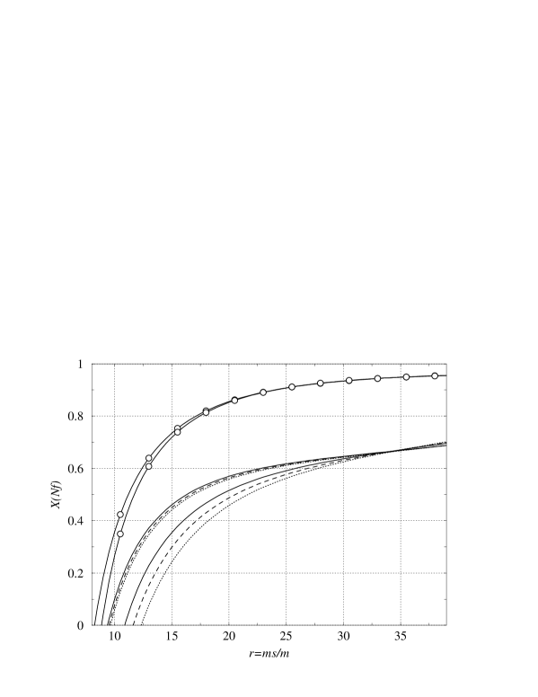
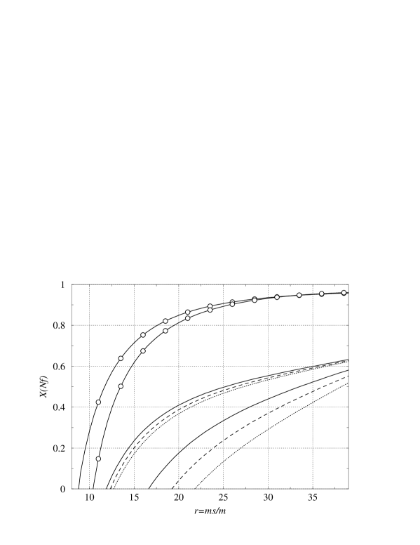
Figure 7: Sum rule : Range for $X(3)$ as a function of $r=m_{s}/m$ for $F_{0}$=85 MeV, with the $T$-matrix models of Refs. [31] (up) and [32] (down). The results are plotted for $s_{1}$=1.2 GeV and $s_{0}$=1.5 GeV (solid lines), 1.6 GeV (dashed lines) and 1.7 GeV (dotted lines). The lines with white circles show the corresponding range for $X(2)$.

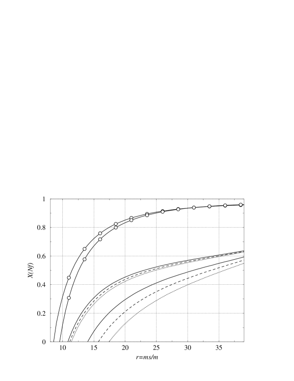
Figure 8: Sum rule : Range for $X(3)$ as a function of $r=m_{s}/m$ for $F_{0}$=85 MeV, with the $T$-matrix models of Ref. [33]. The results are plotted for $s_{1}$=1.2 GeV and $s_{0}$=1.5 GeV (solid lines), 1.6 GeV (dashed lines) and 1.7 GeV (dotted lines). The lines with white circles show the corresponding range for $X(2)$.

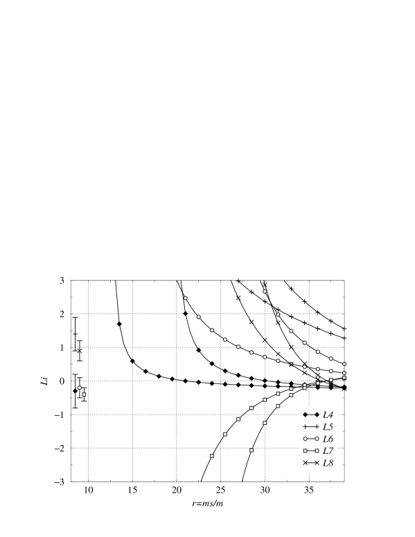
Figure 9: Sum rule : Low-energy constants $L_{i=4\ldots 8}(M_{\rho})\cdot 10^{3}$ as functions of $r=m_{s}/m$ for $F_{0}$=85 MeV, $s_{1}$=1.2 GeV and $s_{0}$=1.6 GeV, with the $T$-matrix models of Refs. [31] (up) and [32] (down). The values plotted on the left, along the vertical axis, are the Standard estimates stemming from Ref. [3].

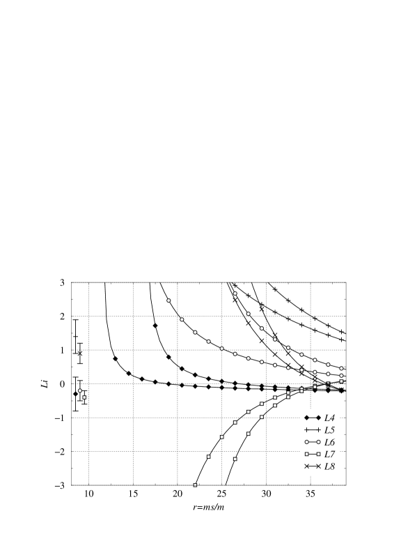
Figure 10: Sum rule : Low-energy constants $L_{i=4\ldots 8}(M_{\rho})\cdot 10^{3}$ as functions of $r=m_{s}/m$ for $F_{0}$=85 MeV, $s_{1}$=1.2 GeV and $s_{0}$=1.6 GeV, with the $T$-matrix models of Refs. [33]. The values plotted on the left, along the vertical axis, are the Standard estimates stemming from Ref. [3].

6.2 Estimate of $X(3)$ and of LEC’s

Hence, two different estimates of $X(2)-X(3)$ are available: the first one is the relation between $X(2)$ and $X(3)$ [Eq. (2.2)], the second one consists of the relation between $X(2)-X(3)$ and $\Pi(0)$ [Eq. (48)] and the sum rule for $\Pi(0)$ [Eq. (5.1)]. In both cases, the difference $X(2)-X(3)$ can be expressed as a function of the observables and of $F_{0},r,X(3)$. This overdertermination can be viewed as a constraint fixing $X(3)$ in terms of $r$ and $F_{0}$, see Figs. 7-8.

This analysis contains 3 sources of errors. i) First, we have neglected NNLO remainders in the expansions of pseudoscalar masses and decay constants. Their effect is easy to control in the relations between $X(2)$ and $X(3)$ [Eq. (2.2)] or $F(2)$ and $F(3)$ [Eq. (39)], but the situation gets more complicated for the sum rule Eq. (48) and for the logarithmic derivatives $\lambda_{P}$ and $\gamma_{P}$. In the framework of Standard $\chi$PT, the authors of Ref. [6] noticed that the dependence on $m_{s}$ of $\Sigma(2)$ is not really affected by two-loop effects. In addition, these effects have the same sign as one-loop contributions: if they were significant, they would increase (and not decrease) the gap between $X(2)$ and $X(3)$. A similar conclusion was drawn in Ref. [18]. The NNLO remainders are supposed here to be small, and they are not included in the results.

ii) The evaluation of the sum rule Eq. (5.1) relies on an estimate of the integral between $s_{1}$ and $s_{0}$. If we choose a couple $(F_{0},r)$, we will not end up with one value for $X(3)$, but rather a range of acceptable values that will also depend on the separators $s_{1}<s_{0}$. On the Figs. 7-8, the upper bound for $X(3)$ remains stable for $\sqrt{s_{0}}>1.5$ GeV, whereas the lower bound depends strongly on $s_{0}$. When $s_{0}$ increases, the lower bound of Eq. (71) is too loose to be saturated. A more stringent lower bound would be welcome.

iii) The third source of error is the $T$-matrix used to build the spectral function Eq. (5.3.2) for $s<s_{1}$. Three different models of $T$-matrix have been used [32, 33, 31]. The central element is the shape of the $f_{0}(980)$ peak. Ref. [31] leads to the least pronounced effect. The two other models [32, 33] lead to a higher $f_{0}(980)$ peak, a larger value for $\Pi(0)$, and a smaller value for $X(3)$.

The range for $X(3)$ is much narrower for large values of $r$, and can be even reduced to one value in the case of Ref. [31]. This range should be broadened if we took into account the errors related to higher orders in the expansion of pseudoscalar masses and decay constants. The value of $F_{0}$ has no major influence on the constraint for $[X(3),r]$. For instance, choosing $F_{0}$=75 MeV would slightly shift the curves for $X(3)$ towards the left of the graphs ($r\to r-2$). Similarly, a change of $\sqrt{s_{1}}$ around 1.2 GeV does not affect strongly the results. If we choose $\sqrt{s_{1}}$=1.3 GeV, the convergence of the upper bound is slightly less good, but its values remain very close to Figs. 7-8. We should add a last comment for $r\sim 25$ (commonly used in the Standard framework): the values of $X(3)$ correspond then to the half of $X(2)$. We end up with a similar result to the one obtained in Refs. [17, 18], but without relying on the hypothesis $X(3)\sim 1$.

The results of the sum rule for $X(3)$ can be converted into bounds for $L_{i=4\ldots 8}$, plotted on Figs. 9-10 as functions of $r$, for $\sqrt{s_{1}}=$ 1.2 GeV, $\sqrt{s_{0}}=$ 1.6 GeV, and $F_{0}=$ 85 MeV. For small $r$, the LEC’s reach very large values: their definition from the low-energy behaviour of QCD correlators includes $1/B_{0}$ factors that make them diverge when $X(3)\to 0$. We notice also the large values of $L_{5}$, $L_{7}$ and $L_{8}$ for $r\sim 25$, because the sum rule pushes $L_{6}(M_{\rho})$ towards slightly positive values. The value of $L_{4}$ is not predicted by the sum rule: it depends essentially on the value fixed for $F_{0}$. For instance, choosing $F_{0}$=75 MeV would yield a slightly positive value for $L_{4}$ as $r$ becomes large.

We have plotted on the left side of Figs. 9-10 the values of the LEC’s of Ref. [3], which were derived assuming that $X(3)$ is of order 1 and $L_{4}(M_{\eta})=L_{6}(M_{\eta})=0$. Let us remind that the values obtained for $L_{5}$, $L_{7}$, and $L_{8}$ are strongly dependent on these assumptions. The values of the LEC’s of Ref. [3] hardly agree with the ones obtained from the sum rule, because the latter leads to positive values of $L_{6}(M_{\rho})$ and to a small three-flavor condensate.

6.3 Slope of the strange scalar form factor of the pion

Additional information about the decay constants is provided by the scalar form factors through a low-energy theorem. Consider the correlator:

$$D^{ij}_{\mu\nu}(p,q)=\lim_{m\to 0}\int\!\!\!\int e^{i(p\cdot x-q\cdot y)}\langle 0|T\{A^{i}_{\mu}(x)\ A^{j}_{\nu}(0)\ \bar{s}s(y)|0\rangle^{(c)},$$ (88)

where $i,j=1\ldots 3$, and $(c)$ denotes the connected part of $(A^{i}_{\mu}A^{j}_{\nu})(\bar{s}s)$. The Ward identities $p^{\mu}D^{ij}_{\mu\nu}=r^{\nu}D^{ij}_{\mu\nu}=0$ (with $r=q-p$) yield the Lorentz decomposition:

$$D^{ij}_{\mu\nu} = m_{s}\delta_{ij}\big{\{}K[r^{2}p_{\mu}p_{\nu}-(p\cdot r)p_{\mu}r_{\nu}+p^{2}r_{\mu}r_{\nu}-p^{2}r^{2}g_{\mu\nu}]$$ (89)

$$\qquad\qquad+L[r_{\mu}p_{\nu}-(p\cdot r)g_{\mu\nu}]\big{\}},$$

where $K$ and $L$ are scalar functions of $p^{2}$, $q^{2}$ and $r^{2}$.

On the one hand, we have:

$$D^{ij}_{\mu\nu}(p,0)=\frac{\partial}{\partial m_{s}}\left[i\int d^{4}xe^{ip\cdot x}\langle 0|T\{A^{i}_{\mu}(x)\ A^{j}_{\nu}(0)\}|0\rangle\right].$$ (90)

The correlator $A^{i}_{\mu}A^{j}_{\nu}$ admits the following decomposition:

$$i\int d^{4}xe^{ip\cdot x}\langle 0|T\{A^{i}_{\mu}(x)\ A^{j}_{\nu}(0)\}|0\rangle=\delta^{ij}[p_{\mu}p_{\nu}-p^{2}g_{\mu\nu}]\Phi(p^{2}).$$ (91)

$\Phi(p^{2})$ contains a pole at $p^{2}=0$ stemming from one-pion states:

$$\Phi(p^{2})=-\frac{F^{2}(2)}{p^{2}}+\ldots$$ (92)

where the dots denote contributions from the other states. We have therefore:

$$D^{ij}_{\mu\nu}(p,0)=-\delta^{ij}[p_{\mu}p_{\nu}-g_{\mu\nu}p^{2}]\left\{\frac{1}{p^{2}}\frac{\partial F^{2}(2)}{\partial m_{s}}+\ldots\right\}.$$ (93)

On the other hand, $T^{ij}_{\mu\nu}$ is dominated at low energy by the exchange of two pions between $\bar{s}s$ and each of the axial currents:

$$D^{ij}_{\mu\nu}=2\delta^{ij}F^{2}(2)G_{1}(q^{2})\frac{p_{\mu}r_{\nu}}{p^{2}r^{2}(p\cdot r)}+\ldots$$ (94)

which contributes to $K$:

$$K(p^{2},q^{2},r^{2})=-2F^{2}(2)\frac{G_{1}(q^{2})}{p^{2}r^{2}(p\cdot r)}+\ldots$$ (95)

whereas $L(p^{2},q^{2},r^{2})$ receives no contribution. We compare Eqs. (93) and (95) for $p,q\to 0$ to obtain:

$$\frac{\partial F^{2}(2)}{\partial m_{s}}=2F^{2}(2)\lim_{q^{2}\to 0}\frac{G_{1}(q^{2})}{q^{2}}\qquad\frac{m_{s}}{F(2)}\frac{\partial F(2)}{\partial m_{s}}=m_{s}G^{\prime}_{1}(0).$$ (96)

This low-energy theorem [17, 18, 26] provides a relation between the logarithmic derivative of $F(2)$ with respect to $m_{s}$, and the slope of the strange scalar form factor of the pion for a vanishing momentum.

We can now exploit the solutions of Omnès-Muskhelishvili equations. According to Eq. (62), we get for the slope of the form factor:

$$m_{s}G^{\prime}_{1}(0)=m_{s}G_{2}(0)B^{\prime}_{1}(0)=m_{s}\frac{\partial\bar{M}_{K}^{2}}{\partial m_{s}}B^{\prime}_{1}(0)=\lambda_{K}M_{K}^{2}B^{\prime}_{1}(0).$$ (97)

$B^{\prime}_{1}(0)$ is computed by taking the derivative with respect to s at 0 of Eq. (61):

$$B^{\prime}_{1}(0)=\frac{1}{\pi}\sum_{j=1}^{2}\int_{4M_{\pi}^{2}}^{\infty}ds^{\prime}\frac{1}{s^{\prime 2}}T_{1j}^{*}(s^{\prime})\sqrt{\frac{s^{\prime}-4M_{j}^{2}}{s^{\prime}}}\theta(s^{\prime}-4M_{j}^{2})B_{j}(s^{\prime}).$$ (98)

The numerical resolution of Omnès-Muskhelishvili equations Eq. (61) yields the values of $\vec{B}(s)$ at the points of integration used for the Gauss-Legendre quadrature [17]. Hence, we can compute directly the integral Eq. (98) by the same integration method.

On the other hand, Eq. (3.1) leads to:

$$\frac{m_{s}}{2F^{2}(2)}\frac{\partial F^{2}(2)}{\partial m_{s}}=\frac{1}{\bar{F}_{\pi}^{2}}\left[m_{s}\tilde{\xi}-\frac{rX(3)}{64\pi^{2}}\frac{F_{\pi}^{2}M_{\pi}^{2}}{F_{0}^{2}}\left(\log\frac{\bar{M}_{K}^{2}}{M_{K}^{2}}+\frac{M_{K}^{2}}{\bar{M}_{K}^{2}}\lambda_{K}\right)\right].$$ (99)

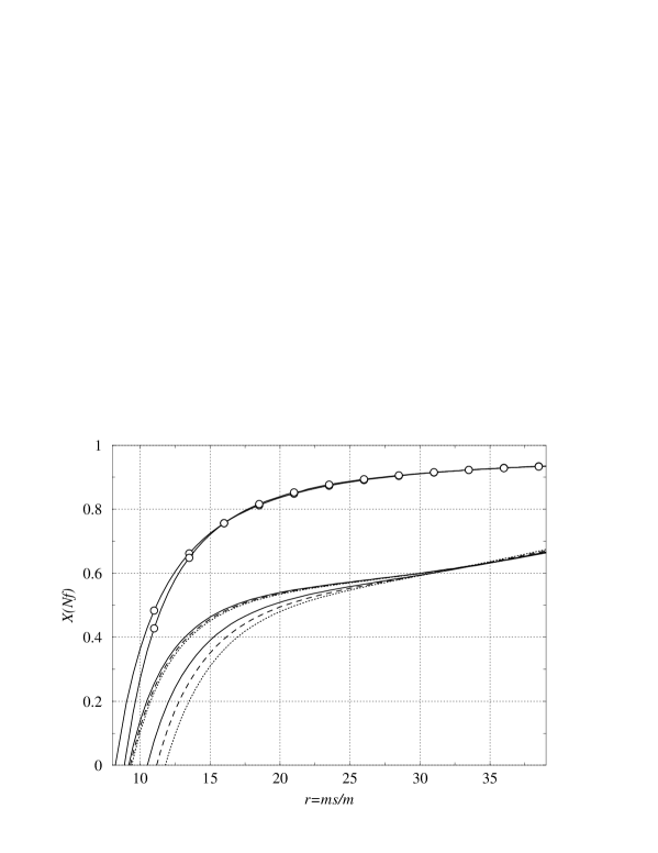
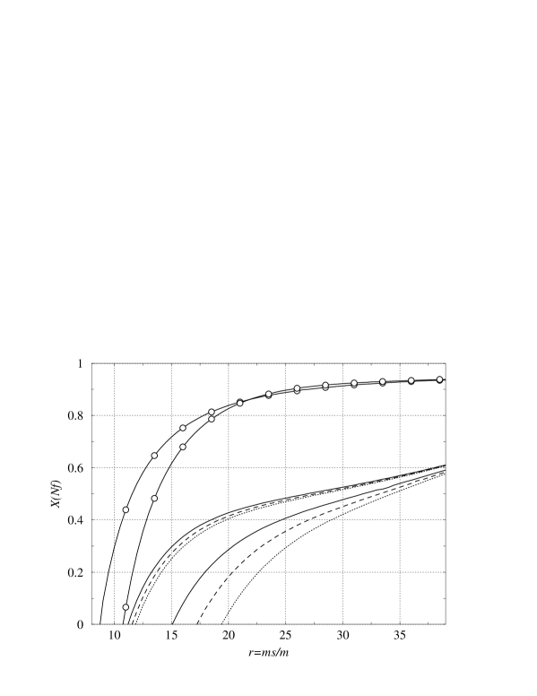
Figure 11: Sum rule and slope of the strange form factor of the pion : Range for $X(3)$ as a function of $r=m_{s}/m$ with the $T$-matrix models of Refs. [31] (up) and [32] (down). The results are plotted for $s_{1}$=1.2 GeV and $s_{0}$=1.5 GeV (solid lines), 1.6 GeV (dashed lines) and 1.7 GeV (dotted lines). The lines with white circles show the corresponding range for $X(2)$.

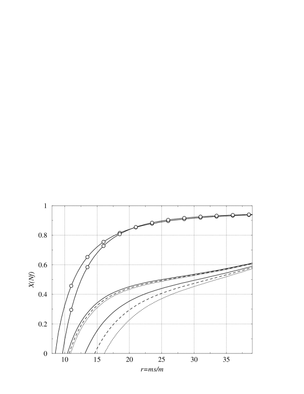
Figure 12: Sum rule and slope of the strange form factor of the pion : Range for $X(3)$ as a function of $r=m_{s}/m$ with the $T$-matrix models of Ref. [33]. The results are plotted for $s_{1}$=1.2 GeV and $s_{0}$=1.5 GeV (solid lines), 1.6 GeV (dashed lines) and 1.7 GeV (dotted lines). The lines with white circles show the corresponding range for $X(2)$.

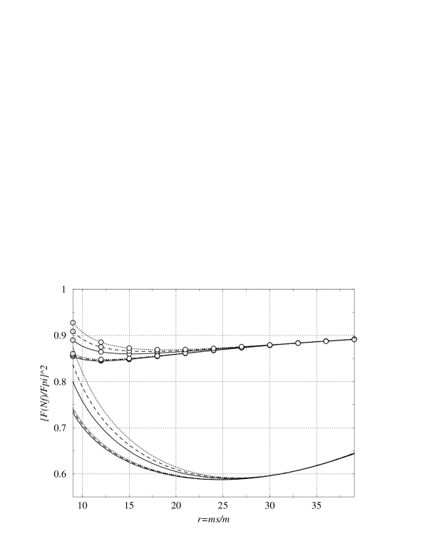
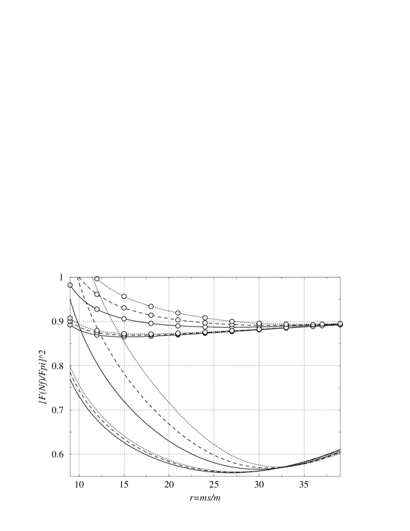
Figure 13: Sum rule and slope of the strange form factor of the pion : Ranges for $[F(3)/F_{\pi}]^{2}$ (no symbol) and $[F(2)/F_{\pi}]^{2}$ (white circles) as functions of $r=m_{s}/m$ with the $T$-matrix models of Refs. [31] (up) and [32] (down). The results are plotted for $s_{1}$=1.2 GeV and $s_{0}$=1.5 GeV (solid lines), 1.6 GeV (dashed lines) and 1.7 GeV (dotted lines).

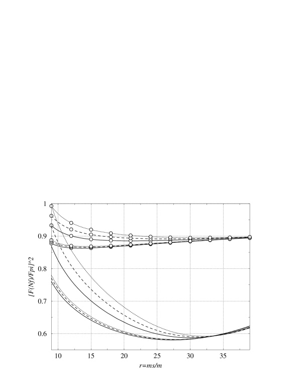
Figure 14: Sum rule and slope of the strange form factor of the pion : Ranges for $[F(3)/F_{\pi}]^{2}$ (no symbol) and $[F(2)/F_{\pi}]^{2}$ (white circles) as functions of $r=m_{s}/m$ with the $T$-matrix model of Refs. [33]. The results are plotted for $s_{1}$=1.2 GeV and $s_{0}$=1.5 GeV (solid lines), 1.6 GeV (dashed lines) and 1.7 GeV (dotted lines).

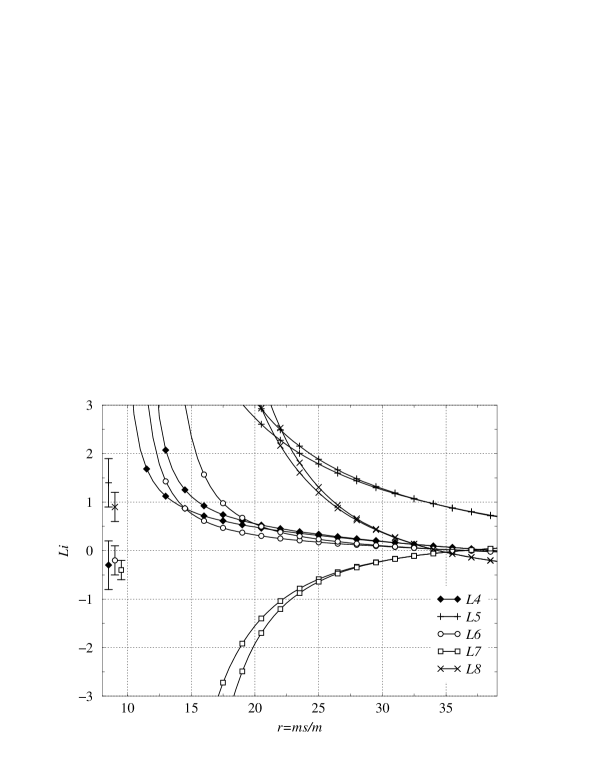
Figure 15: Sum rule and slope of the strange form factor of the pion : Low-energy constants $L_{i=4\ldots 8}(M_{\rho})\cdot 10^{3}$ as functions of $r=m_{s}/m$ for $F_{0}$=85 MeV, $s_{1}$=1.2 GeV and $s_{0}$=1.6 GeV, with the $T$-matrix models of Refs. [31] (up) and [32] (down). The values plotted on the left, along the vertical axis, are the Standard estimates stemming from Ref. [3].

Figure 16: Sum rule and slope of the strange form factor of the pion : Low-energy constants $L_{i=4\ldots 8}(M_{\rho})\cdot 10^{3}$ as functions of $r=m_{s}/m$ for $F_{0}$=85 MeV, $s_{1}$=1.2 GeV and $s_{0}$=1.6 GeV, with the $T$-matrix model of Ref. [33]. The values plotted on the left, along the vertical axis, are the Standard estimates stemming from Ref. [3].

We see that Eq. (96) is an additional constraint, different from the sum rule Eq. (5.1). From the analysis of the pseudoscalar spectrum, we have concluded that all the quantities could be expressed (at the NLO) as functions of masses, decay constants, and 3 parameters $F_{0},r,X(3)$. The sum rule was a first constraint, fixing a range for $X(3)$ depending on $r$ and $F_{0}\equiv F(3)$. If we exploit the second constraint Eq. (96), we can obtain ranges for $F(3)$ and $X(3)$ as functions of $r$, plotted respectively in Figs. 11-12 and Figs. 13-14. These results can also be converted into values for the low-energy constants (see Figs. 15 and 16).

The values of $X(3)$ are close to the ones obtained by the only application of the sum rule Eq. (5.1). The results obtained then for $X(3)$ were not very sensitive to the valued chosen for $F_{0}$. We see also that the slope of the strange scalar form factor of the pion leads to rather small values for $F(3)\equiv F_{0}$ (around 70 MeV) for $r\sim 25$. This result is in agreement with the small positive values obtained for $L_{4}(M_{\rho})$. This increase of $L_{4}$ (with respect to the previous analysis) comes with a decrease of $L_{5}$. In Ref. [26], the analysis of the same form factor led to $d_{F}=m_{s}/F(2)\cdot\partial\log F(2)/\partial m_{s}=0.09$. In the framework of Standard $\chi$PT, such a value corresponds to $L_{4}(M_{\rho})\simeq 0.4\cdot 10^{-3}$, i.e. $F(3)$ of order 75 MeV. This question has also been discussed in Refs. [17, 18, 27].

However, these two constraints do not demand the same accuracy for the scalar form factors. The sum rule involves the integral of the spectral function $\mathrm{Im}\ \Pi$ up to 1.2 GeV, which is dominated by the $f_{0}(980)$ peak. The global shape of the spectral function (and more precisely around 1 GeV) is the crucial element. For the low-energy theorem, we are interested in the slope of a form factor at zero, i.e. low-energy details. The resulting constraint may be less stable than the sum rule. It seemed therefore preferable to split the analysis in two parts: the first one dealing only with the sum rule, the second one exploiting both constraints at the same time.

6.4 Scalar radius of the pion

The scalar radius of the pion $\langle r^{2}\rangle^{\pi}_{s}$ can also be obtained from the scalar form factors of the pion, considered out of the chiral limit [i.e. with the physical masses $m_{s}$ and $m=(m_{u}+m_{d})/2$]:

$$F_{1}(s)=F_{1}(0)\left[1+\frac{1}{6}\langle r^{2}\rangle^{\pi}_{s}s+c_{\pi}s^{2}+\ldots\right],$$ (100)

If we project $\vec{F}$ on the two solutions $\vec{A}$ and $\vec{B}$, we obtain:

$$\langle r^{2}\rangle^{\pi}_{s}=6\frac{F^{\prime}_{1}(0)}{F_{1}(0)}=6\left[A^{\prime}_{1}(0)+\frac{M_{K}^{2}}{M_{\pi}^{2}}\frac{\tilde{\gamma}_{K}}{\tilde{\gamma}_{\pi}}B^{\prime}_{1}(0)\right],$$ (101)

where a third kind of logarithmic derivatives is involved (considered out of the chiral limit): $\tilde{\gamma}_{P}=\partial[\log M_{P}^{2}]/\partial[\log m]$. App. C.2 collects their expressions in terms of the low-energy constants.

We are interested in a quantity describing the non-strange pion form factor around the threshold. It should be possible to neglect the $K\bar{K}$ channel with no major change in the results. This point of view is supported by a numerical estimate: $B^{\prime}_{1}(0)/A^{\prime}_{1}(0)\sim 0.1$ and $(M_{K}^{2}/M_{\pi}^{2})\times(\tilde{\gamma}_{K}/\tilde{\gamma}\pi)\sim 1/2$. If we restricted our analysis to the $\pi\pi$ channel, only the first term (the solution $\vec{A}$) would appear on the right side of Eq. (101). The scalar radius of the pion would be independent of $r$, $X(3)$ and $F_{0}$ in that case. Actually, the second term on the right side of Eq. (101), related to the $K\bar{K}$ channel, is responsible for a weak dependence of $\langle r^{2}\rangle^{\pi}_{s}$ on $r$, $X(3)$, $F_{0}$. We can use the previous results, where $X(3)$ and $F_{0}$ are functions of $r$, in order to study the range of variation for the pion scalar radius:

0.537 – 0.588 $\mathrm{fm}^{2}$		Oller-Oset-Pelaez	Ref. [31],
0.567 – 0.630 $\mathrm{fm}^{2}$		Au-Morgan-Pennington	Ref. [32],
0.592 – 0.650 $\mathrm{fm}^{2}$		Kaminski-Lesniak-Maillet	Ref. [33],

to be compared to the estimates: $0.6\pm 0.2\ \mathrm{fm}^{2}$ [37], $0.55\pm 0.15\ \mathrm{fm}^{2}$ [1], 0.55 to 0.61 $\mathrm{fm}^{2}$ [30], 0.57 to 0.61 $\mathrm{fm}^{2}$ [38] and $0.61\pm 0.04\ \mathrm{fm}^{2}$ [39]. Notice that the matching of Roy equations with Standard $\chi$PT [39] relies strongly on the value of the scalar radius of the pion.

Information about the scalar radius of the pion could be seen as an additional constraint on our system, since $\langle r^{2}\rangle^{\pi}_{s}$ is related to $2L_{4}+L_{5}$. The situation is similar to $d_{F}$: this kind of constraint could rather easily be affected by higher-order corrections. We are also obliged to consider it out of the chiral limit $m\to 0$. It seems therefore wiser not to use this constraint, until a new analysis would treat less crudely NNLO remainders.

7 Conclusions

The LEC’s of the effective chiral Lagrangian should be determined as accurately as possible in order to know and understand the pattern of SB$\chi$S. These constants have generally been estimated from the expansion of Goldstone boson observables in powers of quark masses, supposing (1) a dominance of the quark condensate and (2) an agreement with the large-$N_{c}$ picture of QCD. But such determinations of the LEC’s could be modified if quantum fluctuations turned out to be significant. A symptom of large quantum fluctuations could be seen in the large violation of the Zweig rule in the scalar channel and in large variations of chiral order parameters (e.g. the quark condensate) from $N_{f}=2$ to $N_{f}=3$.

First we have studied how the relaxation of the Standard assumptions (1) and (2) could affect the determination of the LEC’s. To reach this goal, we have studied the expansion in quark masses of the Goldstone boson masses and decay constants. We have truncated these expansions to keep the first two powers in quark masses and we have supposed that higher-order remainders [$O(m_{\mathrm{quark}}^{3})$ for $F_{P}^{2}M_{P}^{2}$ and $O(m_{\mathrm{quark}}^{2})$ for $F_{P}^{2}$] are small. These expansions can be written using “effective” scale-independent constants that combine chiral logarithms and LEC’s. $F_{P}^{2}M_{P}^{2}$ involves $\Sigma(3)$, $F^{2}(3)$ and constants related to $L_{6}$, $L_{7}$ and $L_{8}$, whereas $F_{P}^{2}$ is expressed in terms of $F^{2}(3)$ and constants corresponding to $L_{4}$ and $L_{5}$.

We have not considered these expansions in one-loop Standard $\chi$PT, since the three-flavor quark condensate $\Sigma(3)$ is not supposed to dominate the expansion of pseudoscalar masses. We have not worked either in tree-level Generalized $\chi$PT, since we have included chiral logarithms. These relations between LEC’s and experimental quantities (masses and decay constants) can be inverted to express $L_{i=4\ldots 8}$ [and therefore $X(2)$ and $F(2)$] as functions of $F(3)$, $r=m_{s}/m$ and $X(3)$. We have then studied a possible competition between the first two orders of the quark mass expansions, by admitting large values for the ZR violating constants $L_{4}$ and $L_{6}$ (larger than the expected values on a basis of large-$N_{c}$ arguments).

The variation of the Gell-Mann–Oakes–Renner ratio $X$ from $N_{f}=2$ to $N_{f}=3$ is governed by $L_{6}$. The equality $X(2)=X(3)$ (saturation of the paramagnetic bound) is realized for $L_{6}(M_{\rho})=-0.21\cdot 10^{-3}$. A three-flavor GOR ratio $X(3)$ much smaller than 1 could be obtained for two different reasons. On the one hand, the ratio of quark masses $r$ may be smaller than 25 ($r<20$), which leads to small values of $X(2)$, and then of $X(3)$ [due to the paramagnetic inequality $X(2)\geq X(3)$]. On the other hand, $L_{6}(M_{\rho})$ may be larger than the value $-0.26\cdot 10^{-3}$ saturating the paramagnetic bound for $X$. A slight shift of $L_{6}(M_{\rho})$ towards positive values leads to a significant decrease of $X(3)$, whereas $X(2)$ remains almost constant and unsuppressed. $X(2)$ could thus be of order 1 and $X(3)$ much smaller than 1, provided that $r$ is large ($r\sim 25$) and the Zweig rule is strongly violated for the correlator defining $L_{6}$.

A similar analysis has been performed for the decay constants. $L_{4}$ tunes the difference between $F^{2}(2)$ and $F^{2}(3)$: the equality is obtained for $L_{4}(M_{\rho})=-0.37\cdot 10^{-3}$. If $L_{4}(M_{\rho})$ is heading for positive values, $F^{2}(2)$ and $F^{2}(3)$ split swiftly. For $r=25$, the saturation of both paramagnetic inequalities [for $F^{2}$ and $X$] yields $X(2)=X(3)=0.9$ and $F(2)=F(3)=87$ MeV. This “ultra-Standard” scenario corresponds to the minimal values of $L_{4}$ and $L_{6}$ (no ZR violation). A slight drift towards positives values could lead to very different chiral structures of the vacuum for $N_{f}=2$ and $N_{f}=3$, corresponding to a significant role of quantum fluctuations in SB$\chi$S.

The pseudoscalar spectrum (masses and decay constants) by itself does not contain enough information to pin down the size of these fluctuations. This effect can however be estimated from experimental data in the scalar channel, through a sum rule. The difference between $X(2)$ and $X(3)$ is related to the correlator $\Pi$ of two scalar densities $\bar{u}u$ and $\bar{s}s$ at vanishing momentum. $\Pi(0)$ can be expressed in terms of a sum rule constituted of three distinct integrals. i) We compute the first one, involving the spectral function $\mathrm{Im}\ \Pi$ up to energies around 1.2 GeV, by solving coupled Omnès-Muskhelishvili equations for the scalar form factors of the pion and the kaon. The solutions depend on the $T$-matrix model used to describe the interactions between $\pi\pi$- and $\bar{K}K$-channels, and on a normalization of the form factors related to the derivatives of $M_{\pi}$ and $M_{K}$ with respect to $m$ and $m_{s}$. ii) The second integral corresponds to the contribution of the spectral function $\mathrm{Im}\ \Pi$ between 1.2 and 1.6 GeV, where we cannot trust the two-channel approximation anymore. A second sum rule is used to estimate roughly this integral. iii) The third integral is performed on a large complex circle, with a large enough radius to rely on the Operator Product Expansion (OPE) of $\Pi$.

The most significant contribution stems from the first integral: the $f_{0}(980)$-peak leads to a large value for $\Pi(0)$, and therefore to an important splitting between $X(2)$ and $X(3)$. If we fix $X(3)$, $r$ and $F(3)$, we know $X(2)$ and the LEC’s $L_{i=4\ldots 8}$, using our previous analysis of the pseudoscalar spectrum. The derivatives of $M_{\pi}$ and $M_{K}$ with respect to $m$ and $m_{s}$ can then be directly computed, since they involve $X(3)$, $r$, $F(3)$ and LEC’s. The sum rule Eq. (5.1) can therefore be seen as a constraint, giving $X(3)$ as a function of $r$ and $F(3)$. Several sources of errors could affect this sum rule : the higher-order remainders in the expansions of $F_{P}^{2}M_{P}^{2}$ and $F_{P}^{2}$, the rough estimate of the integral in the intermediate energy range, the $T$-matrix model. The three models considered here support nevertheless a large decrease of $X(3)$ with respect to $X(2)$, corresponding to positive values of $L_{6}(M_{\rho})$. The size of the splitting between the quark condensates depends on the height of the $f_{0}(980)$ peak in the spectral function. In the particular case of ”Standard” inputs $r\sim 25$, $F_{0}=85$ MeV, the results of Ref. [17] are confirmed: $X(3)$ can hardly reach more than one half of $X(2)$ for the three considered models.

The scalar form factors of the pion and the kaon can be exploited in several different ways. For instance, $L_{4}$ [i.e. $F(3)$] is related to the slope of the scalar form factor of the pion at zero. This second constraint may be used to fix $X(3)$ and $F_{0}$ as functions of $r$. If the conclusions for $X(3)$ remain unchanged, positive values of $L_{4}(M_{\rho})$ are obtained, leading to a significant decrease from $F(2)$ to $F(3)$ (20 to 30%). The Zweig rule would be violated strongly for $L_{4}$ and $L_{6}$. However, this second constraint is sensitive to fine details of a form factor (slope at zero), whereas the sum rule depends on the general shape of the spectral function $\mathrm{Im}\ \Pi$ [and especially on the presence of a high peak corresponding to the $f_{0}(980)$ resonance]. The scalar radius of the pion has also been computed, in agreement with former estimates.

A large decrease of the quark condensate from 2 to 3 flavors could be understood in terms of chiral phase transitions [13]. One of these transitions could be triggered by a vanishing quark condensate. If the corresponding critical value $n_{\mathrm{crit}}(N_{c})$ turned out to be close to 2-3, we should expect significant variations of the quark condensate with $N_{f}$ in the vicinity of the critical point. Moreover, in terms of eigenmodes of the Dirac operator, the quark condensate can be interpreted as a density of eigenvalues, whereas $L_{6}$ corresponds to fluctuations of this density. Near the critical point where the first vanishes, the latter is expected to increase significantly. Let us remind that this scenario is only a possible explanation for a large difference between $X(2)$ and $X(3)$. The large value of ZR violating LEC’s might be caused by another (and unrelated) mechanism.

Forthcoming experiments [40] on $\pi\pi$ scattering should pin down the value of $X(2)$, which is strongly correlated to $r$. If $X(2)$ turned out to be close to 1, they could also measure low-energy constants of the SU(2)$\times$SU(2) Lagrangian, $l_{3}$ and $l_{4}$ [1, 41]. However, these experimental values could not be used to fix SU(3)$\times$SU(3) LEC’s without assumptions on the size of the ZR violating LEC’s $L_{4}$ and $L_{6}$ [13]. It would be possible to constrain more tightly $L_{6}$ through a more sophisticated analysis of the sum rule including bounds on $X(2)$ (or equivalently $r$). However, this remains a very indirect determination of the three-flavor condensate. Direct experimental tests are necessary to investigate closely the chiral structure of QCD vacuum for three massless quarks, and to understand the role of quantum fluctuations in the pattern of SB$\chi$S.

Appendix A Spectrum of pseudoscalar mesons

A.1 Decay constants

The decay constants are [1, 36] :

$$F_{\pi}^{2} = F_{0}^{2}+2m\xi+2(2m+m_{s})\tilde{\xi}$$

$$\quad+\frac{1}{16\pi^{2}}\frac{F_{\pi}^{2}M_{\pi}^{2}}{F_{0}^{2}}X(3)\left[2\log\frac{M_{K}^{2}}{M_{\pi}^{2}}+\log\frac{M_{\eta}^{2}}{M_{K}^{2}}\right]+\varepsilon_{\pi},$$

$$F_{K}^{2} = F_{0}^{2}+(m+m_{s})\xi+2(2m+m_{s})\tilde{\xi}$$

$$\quad+\frac{1}{2}\frac{F_{\pi}^{2}M_{\pi}^{2}}{F_{0}^{2}}X(3)L+\varepsilon_{K},$$

$$F_{\eta}^{2} = F_{0}^{2}+\frac{2}{3}(m+2m_{s})\xi+2(2m+m_{s})\tilde{\xi}$$

$$\quad+\frac{1}{48\pi^{2}}\frac{F_{\pi}^{2}M_{\pi}^{2}}{F_{0}^{2}}(2r+1)X(3)\log\frac{M_{\eta}^{2}}{M_{K}^{2}}+\varepsilon_{\eta},$$

with the scale-independent low-energy constants:

$$\xi = F_{0}^{2}\xi(\mu)-\frac{B_{0}}{32\pi^{2}}\left(\log\frac{M_{K}^{2}}{\mu^{2}}+2\log\frac{M_{\eta}^{2}}{\mu^{2}}\right)$$ (105)

$$= 8B_{0}\left[L_{5}(\mu)-\frac{1}{256\pi^{2}}\left(\log\frac{M_{K}^{2}}{\mu^{2}}+2\log\frac{M_{\eta}^{2}}{\mu^{2}}\right)\right],$$ (106)

$$\tilde{\xi} = F_{0}^{2}\tilde{\xi}(\mu)-\frac{B_{0}}{32\pi^{2}}\log\frac{M_{K}^{2}}{\mu^{2}}$$ (107)

$$= 8B_{0}\left[L_{4}(\mu)-\frac{1}{256\pi^{2}}\log\frac{M_{K}^{2}}{\mu^{2}}\right],$$ (108)

and:

$$L=\frac{1}{32\pi^{2}}\left[3\log\frac{M_{K}^{2}}{M_{\pi}^{2}}+\log\frac{M_{\eta}^{2}}{M_{K}^{2}}\right].$$ (109)

The higher-order contributions are denoted by $\delta_{2}F_{P}^{2}$. The effective constants are related to $F_{0}$ through the relations:

$$m_{s}\xi = \frac{r}{r-1}\left\{F_{K}^{2}-F_{\pi}^{2}\right.$$

$$\qquad\left.+\frac{1}{64\pi^{2}}\frac{F_{\pi}^{2}M_{\pi}^{2}}{F_{0}^{2}}X(3)\left[5\log\frac{M_{K}^{2}}{M_{\pi}^{2}}+3\log\frac{M_{\eta}^{2}}{M_{K}^{2}}\right]\right\}$$

$$+\frac{r}{r-1}\left[\varepsilon_{\pi}-\varepsilon_{K}\right],$$

$$m_{s}\tilde{\xi} = \frac{r}{2(r+2)}\left\{\frac{r+1}{r-1}F_{\pi}^{2}-\frac{2}{r-1}F_{K}^{2}-F_{0}^{2}\right.$$

$$\qquad\left.-\frac{1}{32\pi^{2}}\frac{F_{\pi}^{2}M_{\pi}^{2}}{F_{0}^{2}}X(3)\left[\frac{4r+1}{r-1}\log\frac{M_{K}^{2}}{M_{\pi}^{2}}+\frac{2r+1}{r-1}\log\frac{M_{\eta}^{2}}{M_{K}^{2}}\right]\right\}$$

$$+\frac{r}{2(r+2)}\left[\frac{2}{r-1}\varepsilon_{K}-\frac{r+1}{r-1}\varepsilon_{\pi}\right].$$

The decay constants fulfill the relation:

$$F_{\eta}^{2} = \frac{4}{3}F_{K}^{2}-\frac{1}{3}F_{\pi}^{2}+\frac{1}{24\pi^{2}}\frac{M_{\pi}^{2}F_{\pi}^{2}}{F_{0}^{2}}rX(3)\log\frac{M_{\eta}^{2}}{M_{K}^{2}}$$

$$\qquad+\frac{1}{48\pi^{2}}\frac{M_{\pi}^{2}F_{\pi}^{2}}{F_{0}^{2}}X(3)\left(\log\frac{M_{\eta}^{2}}{M_{K}^{2}}-\log\frac{M_{K}^{2}}{M_{\pi}^{2}}\right)$$

$$\qquad+\varepsilon_{\eta}-\frac{4}{3}\varepsilon_{K}+\frac{1}{3}\varepsilon_{\pi}.$$

A.2 Masses

The pseudoscalar masses are [1, 36]:

$$F_{\pi}^{2}M_{\pi}^{2} = 2m\Sigma+(2mm_{s}+4m^{2})Z^{S}+4m^{2}A$$

$$\quad+\frac{F_{\pi}^{4}M_{\pi}^{4}}{F_{0}^{4}}[X(3)]^{2}L+F_{\pi}^{2}\delta_{\pi},$$

$$F_{K}^{2}M_{K}^{2} = (m_{s}+m)\Sigma+(m_{s}+m)(m_{s}+2m)Z^{S}+(m_{s}+m)^{2}A$$

$$\quad+\frac{1}{4}\frac{F_{\pi}^{4}M_{\pi}^{4}}{F_{0}^{4}}(r+1)[X(3)]^{2}L+F_{K}^{2}\delta_{K},$$

$$F_{\eta}^{2}M_{\eta}^{2} = \frac{2}{3}(2m_{s}+m)\Sigma+\frac{2}{3}(2m_{s}+m)(m_{s}+2m)Z^{S}$$

$$\quad+\frac{4}{3}(2m^{2}_{s}+m^{2})A+\frac{8}{3}(m_{s}-m)^{2}Z^{P}$$

$$\quad+\frac{1}{3}\frac{F_{\pi}^{4}M_{\pi}^{4}}{F_{0}^{4}}[X(3)]^{2}L+F_{\eta}^{2}\delta_{\eta}.$$

with the scale-independent low-energy constants:

$$Z^{S} = 2F^{2}_{0}Z_{0}^{S}(\mu)-\frac{B_{0}^{2}}{32\pi^{2}}\left\{2\log\frac{M_{K}^{2}}{\mu^{2}}+\frac{4}{9}\log\frac{M_{\eta}^{2}}{\mu^{2}}\right\}$$ (116)

$$= 32B_{0}^{2}\left[L_{6}(\mu)-\frac{1}{512\pi^{2}}\left\{\log\frac{M_{K}^{2}}{\mu^{2}}+\frac{2}{9}\log\frac{M_{\eta}^{2}}{\mu^{2}}\right\}\right],$$ (117)

$$A = F^{2}_{0}A_{0}(\mu)-\frac{B_{0}^{2}}{32\pi^{2}}\left\{\log\frac{M_{K}^{2}}{\mu^{2}}+\frac{2}{3}\log\frac{M_{\eta}^{2}}{\mu^{2}}\right\}$$ (118)

$$= 16B_{0}^{2}\left[L_{8}(\mu)-\frac{1}{512\pi^{2}}\left\{\log\frac{M_{K}^{2}}{\mu^{2}}+\frac{2}{3}\log\frac{M_{\eta}^{2}}{\mu^{2}}\right\}\right],$$ (119)

$$Z^{P} = F^{2}_{0}Z_{0}^{P}=16B_{0}^{2}L_{7}.$$ (120)

The higher-order remainders are denoted by $\delta M_{P}^{2}$. The low-energy constants can be estimated using the relations:

$$m_{s}^{2}Z^{S} = F_{\pi}^{2}M_{\pi}^{2}\frac{r^{2}}{2(r+2)}$$

$$\quad\times\left\{1-\tilde{\epsilon}(r)-X(3)-\frac{1}{32\pi^{2}}\frac{F_{\pi}^{2}M_{\pi}^{2}}{F_{0}^{4}}\frac{r[X(3)]^{2}}{r-1}L\right\}$$

$$+\frac{r^{2}}{2(r+2)}\left[\frac{4}{r^{2}-1}F_{K}^{2}\delta_{K}-\frac{r+1}{r-1}F_{\pi}^{2}\delta_{\pi}\right],$$

$$m_{s}^{2}A = F_{\pi}^{2}M_{\pi}^{2}\frac{r^{2}}{4}\left\{\tilde{\epsilon}(r)+\frac{1}{32\pi^{2}}\frac{F_{\pi}^{2}M_{\pi}^{2}}{F_{0}^{4}}\frac{[X(3)]^{2}}{r-1}L\right\}$$

$$+\frac{r^{2}}{2(r-1)}F_{\pi}^{2}\delta_{\pi}-\frac{r^{2}}{r^{2}-1}F_{K}^{2}\delta_{K},$$

$$m_{s}^{2}Z^{P} = \frac{r^{2}}{8}\left\{\frac{1}{(r-1)^{2}}\left[3F_{\eta}^{2}M_{\eta}^{2}+F_{\pi}^{2}M_{\pi}^{2}-4F_{K}^{2}M_{K}^{2}\right]-F_{\pi}^{2}M_{\pi}^{2}\tilde{\epsilon}(r)\right\}$$ (123)

$$-\frac{r^{2}}{8(r-1)^{2}}\left[3F_{\eta}^{2}\delta_{\eta}+\frac{8r}{r+1}F_{K}^{2}\delta_{K}+(2r-1)F_{\pi}^{2}\delta_{\pi}\right],$$

with:

$$\tilde{\epsilon}(r)=2\frac{\tilde{r}_{2}-r}{r^{2}-1}\qquad\tilde{r}_{2}=2\frac{F_{K}^{2}M_{K}^{2}}{F_{\pi}^{2}M_{\pi}^{2}}-1.$$ (124)

A.3 Pseudoscalar masses for $m\to 0$

From the previous relations, one can derive low-energy constants from experimental data (pseudoscalar masses, $F_{\pi}$ and $F_{K}$) and 3 parameters: $r$, $X(3)$ and $F_{0}$.

$$\begin{array}[]{rcccl}F_{\pi},F_{K}&\to&F_{\eta},m_{s}\xi,m_{s}\tilde{\xi}&\to&\bar{F}_{\pi},\bar{F}_{K},\bar{F}_{\eta}\\ M_{\pi},M_{K},M_{\eta}&\to&m_{s}^{2}Z^{S},m_{s}^{2}A,m_{s}^{2}Z^{P}&\to&\bar{M}_{K},\bar{M}_{\eta}\end{array}$$ (125)

In the chiral limit $m\to 0$, we will have to know the effective constants:

$$\lim_{m\to 0}X_{i}=X_{i}+\sum_{P}C_{P}\cdot\log\frac{\bar{M}_{P}^{2}}{M_{P}^{2}}.$$ (126)

To compute $\bar{M}_{P}$ in this expression, we take the chiral limit of the mass expansions Eqs. (A.2)-(A.2). But these expansions involve the effective constants at $m=0$, which leads to corrections containing logarithms of $\bar{M}_{Q}/M_{Q}$:

$$\bar{M}_{P}=\sum_{i}a_{i}X_{i}+\sum_{Q}D_{Q}\cdot\log\frac{\bar{M}_{Q}^{2}}{M_{Q}^{2}}.$$ (127)

The equations Eq. (127) could be solved iteratively. Actually, $\bar{M}_{Q}/M_{Q}$ remains very close to 1. The calculation is simplified (and still accurate) if we compute in a slightly different way $\bar{M}_{Q}$ in the logarithmic piece of Eq. (127). We start from Eq. (127), and we neglect the second (logarithmic) term:

$$\bar{M}_{Q}=\sum_{i}a_{i}X_{i}.$$ (128)

$\bar{M}_{Q}$ is then directly computed from observables and $F_{0},r,X(3)$. We put then these values of $\bar{M}_{Q}$ in the logarithmic term of Eq. (127). We end up with values of $\bar{M}_{P}$ very close to the ones computed iteratively. These values will be used to compute the low-energy constants in the chiral limit $X_{i}|_{m=0}$ using Eq. (126).

Appendix B Operator Product Expansion for $\Pi$

Six integrals contribute to the Wilson coefficient of $m_{s}\langle\bar{u}u\rangle$ at the leading order in the strong coupling constant. The corresponding Feynman diagrams are drawn on Fig. 5. On each line, the left and right diagrams correspond to each other by crossing the gluonic lines. A simple change of variables in the integrals shows that the diagrams on the same line contribute identically to the Wilson coefficient.

We want to consider the large-$p^{2}$ behavior of integrals like:

$$J(\{\nu_{i}\},\{m_{i}\},p)=\int\frac{d^{4}q\ d^{4}k}{[q^{2}-m_{1}^{2}]^{\nu_{1}}[k^{2}-m_{2}^{2}]^{\nu_{2}}}$$ (129)

$$\qquad\times\frac{1}{[(k+q)^{2}-m_{3}^{2}]^{\nu_{3}}[(p-q)^{2}-m_{4}^{2}]^{\nu_{4}}[(k+p)^{2}-m_{5}^{2}]^{\nu_{5}}}.$$

These integrals are formally identical to the integrals arising in two-loop computations of self-energies, see Fig. 17.

Figure 17: Self-energy diagram, leading to the same kind of integrals as in the OPE of $\Pi$ at the lowest order.

The behavior of such integrals at large external momentum is known. The basic idea is to follow the flow of this large external momentum through the Feynman diagram, in order to Taylor expand correctly the propagators [24]. This procedure relies on the asymptotic expansion theorem [25] and can be formally expressed as:

$$J_{\Gamma}{\displaystyle\mathop{\sim}_{p^{2}\to\infty}}\sum_{\gamma}J_{\Gamma/\gamma}\circ\mathcal{T}_{\{m_{i}\},\{q_{i}\}}J_{\gamma}.$$ (130)

$\Gamma$ denotes the whole graph, $\gamma$ are subgraphs into which the large external momentum may flow and $\Gamma/\gamma$ is the complementary graph of $\gamma$. For each subgraph $\gamma$ (see Fig. 18), we write the corresponding Feynman integral $J_{\gamma}$. We perform then a Taylor expansion $\mathcal{T}_{\{m_{i}\},\{q_{i}\}}$ with respect to the masses and the small momenta (external to $\gamma$ and not containing $p$). We combine the resulting “expanded” integral with the remaining graph $\Gamma/\gamma$ and integrate over internal momenta. The asymptotic behavior of the whole integral $J_{\Gamma}$ is obtained by considering all the possible flows $\gamma$ for the large external momentum.

Figure 18: Subgraphs involved in the asymptotic expansion of the two-loop Feynman integrals. The solid lines constitute the subgraphs, the dashed lines correspond to the excluded propagators [24].

We look for the leading order in $1/p^{2}$ of the Wilson coefficient. All the subraphs do not contribute with the same power of $1/p^{2}$. In particular, the diagrams of type 5 do not appear in the Wilson coefficient of $m_{s}\langle\bar{u}u\rangle$ at the leading order in $1/p^{2}$. Gathering all the contributions, we obtain:

$$\Pi(p^{2}){\displaystyle\mathop{\sim}_{P^{2}\to\infty}}\frac{\alpha_{s}^{2}m_{s}^{2}}{M_{\pi}^{2}M_{K}^{2}}\frac{2}{\pi^{2}p^{2}}\{[5-6\zeta(3)]+[5-6\zeta(3)]-[1+6\zeta(3)]\},$$ (131)

where the bracketed terms correspond respectively to the contributions of the first, second and third lines in Fig. 5. The $\zeta(3)$ terms are related to subdiagrams of type 1 (see Fig. 18), corresponding to two-loop massless integrals $J(\{\nu_{i}\},\{0\},p)$.

Appendix C Logarithmic derivatives

C.1 Logarithmic derivatives for $m\to 0$

To compute the logarithmic derivatives $\gamma_{P}$ and $\lambda_{P}$:

$$\gamma_{P}=\frac{m}{M_{P}^{2}}\left(\frac{\partial M_{P}^{2}}{\partial m}\right)_{m=0},\qquad\lambda_{P}=\frac{m_{s}}{M_{P}^{2}}\left(\frac{\partial M_{P}^{2}}{\partial m_{s}}\right)_{m=0},$$ (132)

we use the relations:

$$\gamma_{P} = \frac{m}{\bar{F}_{P}^{2}M_{P}^{2}}\left(\frac{\partial[F_{P}^{2}M_{P}^{2}]}{\partial m}\right)_{m=0}\!\!\!-\frac{\bar{M}_{P}^{2}}{M_{P}^{2}}\cdot\frac{m}{\bar{F}_{P}^{2}}\left(\frac{\partial F_{P}^{2}}{\partial m}\right)_{m=0},$$ (133)

$$\lambda_{P} = \frac{m_{s}}{\bar{F}_{P}^{2}M_{P}^{2}}\frac{\partial[\bar{F}_{P}^{2}\bar{M}_{P}^{2}]}{\partial m_{s}}-\frac{\bar{M}_{P}^{2}}{M_{P}^{2}}\cdot\frac{m_{s}}{\bar{F}_{P}^{2}}\frac{\partial\bar{F}_{P}^{2}}{\partial m_{s}},$$ (134)

where $\bar{X}=\lim_{m\to 0}X$.

The logarithmic derivatives with respect to $m$ are:

$$\gamma_{\pi} = \frac{1}{\bar{F}_{\pi}^{2}M_{\pi}^{2}}\left\{F_{\pi}^{2}M_{\pi}^{2}X(3)+\frac{2}{r}m_{s}^{2}Z^{S}\right.$$

$$\quad\left.-\frac{1}{32\pi^{2}}\frac{F_{\pi}^{4}M_{\pi}^{4}}{F_{0}^{4}}r[X(3)]^{2}\left(\log\frac{\bar{M}_{K}^{2}}{M_{K}^{2}}+\frac{2}{9}\log\frac{\bar{M}_{\eta}^{2}}{M_{\eta}^{2}}\right)\right\}$$

$$+\frac{m}{\bar{F}_{\pi}^{2}M_{\pi}^{2}}\left(\frac{\partial[F_{\pi}^{2}\delta_{\pi}]}{\partial m}\right)_{m=0},$$

$$\gamma_{K}\left[1-\frac{3}{64\pi^{2}}\frac{F_{\pi}^{2}M_{\pi}^{2}}{F_{0}^{2}\bar{F}_{K}^{2}}rX(3)+\frac{3}{128\pi^{2}}\frac{M_{\pi}^{4}F_{\pi}^{4}}{F_{0}^{4}}\frac{1}{\bar{F}_{K}^{2}\bar{M}_{K}^{2}}[rX(3)]^{2}\right]$$

$$\quad+\gamma_{\eta}\left[-\frac{1}{32\pi^{2}}\frac{F_{\pi}^{2}M_{\pi}^{2}}{F_{0}^{2}\bar{F}_{K}^{2}}\frac{M_{\eta}^{2}\bar{M}_{K}^{2}}{\bar{M}_{\eta}^{2}M_{K}^{2}}rX(3)+\frac{5}{576\pi^{2}}\frac{M_{\pi}^{4}F_{\pi}^{4}}{F_{0}^{4}}\frac{1}{\bar{F}_{K}^{2}M_{K}^{2}}\frac{M_{\eta}^{2}}{\bar{M}_{\eta}^{2}}[rX(3)]^{2}\right]$$

$$=\frac{1}{\bar{F}_{K}^{2}M_{K}^{2}}\left\{\frac{F_{\pi}^{2}M_{\pi}^{2}}{2}X(3)+\frac{1}{r}\left[3m_{s}^{2}Z^{S}+2m_{s}^{2}A-\bar{M}_{K}^{2}\left(m_{s}\xi+4m_{s}\tilde{\xi}\right)\right]\right.$$

$$\qquad\qquad-\frac{1}{16\pi^{2}}\frac{F_{\pi}^{4}M_{\pi}^{4}}{F_{0}^{4}}r[X(3)]^{2}\left[\log\frac{\bar{M}_{K}^{2}}{M_{K}^{2}}+\frac{1}{3}\log\frac{\bar{M}_{\eta}^{2}}{M_{\eta}^{2}}\right]$$

$$\qquad\qquad\left.+\frac{1}{64\pi^{2}}\frac{F_{\pi}^{2}M_{\pi}^{2}}{F_{0}^{2}}\bar{M}_{K}^{2}X(3)\left[5\log\frac{\bar{M}_{K}^{2}}{M_{K}^{2}}+2\log\frac{\bar{M}_{\eta}^{2}}{M_{\eta}^{2}}\right]\right\}$$

$$\quad+\frac{m}{\bar{F}_{K}^{2}M_{K}^{2}}\left(\frac{\partial[F_{K}^{2}\delta_{K}]}{\partial m}\right)_{m=0}\!\!\!-\frac{\bar{M}_{K}^{2}}{M_{K}^{2}}\cdot\frac{m}{\bar{F}_{K}^{2}}\left(\frac{\partial\varepsilon_{K}}{\partial m}\right)_{m=0},$$ (136)

$$\gamma_{K}\left[-\frac{3}{32\pi^{2}}\frac{F_{\pi}^{2}M_{\pi}^{2}}{F_{0}^{2}\bar{F}_{\eta}^{2}}\frac{M_{K}^{2}\bar{M}_{\eta}^{2}}{\bar{M}_{K}^{2}M_{\eta}^{2}}rX(3)+\frac{1}{24\pi^{2}}\frac{F_{\pi}^{4}M_{\pi}^{4}}{F_{0}^{4}}\frac{1}{\bar{F}_{\eta}^{2}M_{\eta}^{2}}\frac{M_{K}^{2}}{\bar{M}_{K}^{2}}[rX(3)]^{2}\right]$$

$$\quad+\gamma_{\eta}\left[1+\frac{1}{54\pi^{2}}\frac{F_{\pi}^{4}M_{\pi}^{4}}{F_{0}^{4}}\frac{1}{\bar{F}_{\eta}^{2}\bar{M}_{\eta}^{2}}[rX(3)]^{2}\right]$$

$$=\frac{1}{\bar{F}_{\eta}^{2}M_{\eta}^{2}}\left\{\frac{F_{\pi}^{2}M_{\pi}^{2}}{3}X(3)\right.$$

$$\qquad\qquad+\frac{1}{r}\left[\frac{10}{3}m_{s}^{2}Z^{S}+\frac{16}{3}m_{s}^{2}Z^{P}-\bar{M}_{\eta}^{2}\left(\frac{2}{3}m_{s}\xi+4m_{s}\tilde{\xi}\right)\right]$$

$$\qquad\qquad-\frac{1}{32\pi^{2}}\frac{F_{\pi}^{4}M_{\pi}^{4}}{F_{0}^{4}}r[X(3)]^{2}\left[\frac{5}{3}\log\frac{M_{K}^{2}}{\bar{M}_{K}^{2}}+\frac{10}{27}\log\frac{M_{\eta}^{2}}{\bar{M}_{\eta}^{2}}\right]$$

$$\left.\qquad\qquad-\frac{1}{32\pi^{2}}\frac{F_{\pi}^{2}M_{\pi}^{2}}{F_{0}^{2}}\bar{M}_{\eta}^{2}X(3)\left[7\log\frac{\bar{M}_{K}^{2}}{M_{K}^{2}}+2\log\frac{\bar{M}_{\eta}^{2}}{M_{\eta}^{2}}+2\log\frac{\bar{M}_{K}^{2}}{\bar{M}_{\eta}^{2}}\right]\right\}$$

$$\quad+\frac{m}{\bar{F}_{\eta}^{2}M_{\eta}^{2}}\left(\frac{\partial[F_{\eta}^{2}\delta_{\eta}]}{\partial m}\right)_{m=0}\!\!\!-\frac{\bar{M}_{\eta}^{2}}{M_{\eta}^{2}}\cdot\frac{m}{\bar{F}_{\eta}^{2}}\left(\frac{\partial\varepsilon_{\eta}}{\partial m}\right)_{m=0}.$$ (137)

The logarithmic derivatives with respect to $m_{s}$ are:

$$\lambda_{\pi}=0,$$ (138)

$$\lambda_{K}\left[1-\frac{3}{64\pi^{2}}\frac{F_{\pi}^{2}M_{\pi}^{2}}{F_{0}^{2}\bar{F}_{K}^{2}}rX(3)+\frac{3}{128\pi^{2}}\frac{F_{\pi}^{4}M_{\pi}^{4}}{F_{0}^{4}}\frac{1}{\bar{F}_{K}^{2}\bar{M}_{K}^{2}}[rX(3)]^{2}\right]$$ (139)

$$\quad+\lambda_{\eta}\left[-\frac{1}{32\pi^{2}}\frac{F_{\pi}^{2}M_{\pi}^{2}}{F_{0}^{2}\bar{F}_{K}^{2}}\frac{\bar{M}_{K}^{2}M_{\eta}^{2}}{M_{K}^{2}\bar{M}_{\eta}^{2}}rX(3)+\frac{5}{576\pi^{2}}\frac{F_{\pi}^{4}M_{\pi}^{4}}{F_{0}^{4}}\frac{1}{\bar{F}_{K}^{2}M_{K}^{2}}\frac{M_{\eta}^{2}}{\bar{M}_{\eta}^{2}}[rX(3)]^{2}\right]$$

$$=\frac{1}{\bar{F}_{K}^{2}M_{K}^{2}}\left\{\frac{F_{\pi}^{2}M_{\pi}^{2}}{2}rX(3)+2m_{s}^{2}Z^{S}+2m_{s}^{2}A-\bar{M}_{K}^{2}(m_{s}\xi+2m_{s}\tilde{\xi})\right.$$

$$\qquad\qquad-\frac{1}{128\pi^{2}}\frac{F_{\pi}^{4}M_{\pi}^{4}}{F_{0}^{4}}[rX(3)]^{2}\left[5\log\frac{\bar{M}_{K}^{2}}{M_{K}^{2}}+\frac{20}{9}\log\frac{\bar{M}_{\eta}^{2}}{M_{\eta}^{2}}\right]$$

$$\left.\qquad\qquad+\frac{1}{64\pi^{2}}\frac{F_{\pi}^{2}M_{\pi}^{2}}{F_{0}^{2}}\bar{M}_{K}^{2}rX(3)\left[3\log\frac{\bar{M}_{K}^{2}}{M_{K}^{2}}+2\log\frac{\bar{M}_{\eta}^{2}}{M_{\eta}^{2}}\right]\right\}$$

$$\quad+\frac{m_{s}}{\bar{F}_{K}^{2}M_{K}^{2}}\left(\frac{\partial[F_{K}^{2}\delta_{K}]}{\partial m_{s}}\right)_{m=0}\!\!\!-\frac{\bar{M}_{K}^{2}}{M_{K}^{2}}\cdot\frac{m_{s}}{\bar{F}_{K}^{2}}\left(\frac{\partial\varepsilon_{K}}{\partial m_{s}}\right)_{m=0},$$

$$\lambda_{K}\left[-\frac{3}{32\pi^{2}}\frac{F_{\pi}^{2}M_{\pi}^{2}}{F_{0}^{2}\bar{F}_{\eta}^{2}}\frac{M_{K}^{2}}{\bar{M}_{K}^{2}}\frac{\bar{M}_{\eta}^{2}}{M_{\eta}^{2}}rX(3)+\frac{1}{24\pi^{2}}\frac{F_{\pi}^{4}M_{\pi}^{4}}{F_{0}^{4}}\frac{1}{\bar{F}_{\eta}^{2}M_{\eta}^{2}}\frac{M_{K}^{2}}{\bar{M}_{K}^{2}}[rX(3)]^{2}\right]$$

$$\quad+\lambda_{\eta}\left[1+\frac{1}{54\pi^{2}}\frac{F_{\pi}^{4}M_{\pi}^{4}}{F_{0}^{4}}\frac{1}{\bar{F}_{\eta}^{2}\bar{M}_{\eta}^{2}}[rX(3)]^{2}\right]$$

$$=\frac{1}{\bar{F}_{\eta}^{2}M_{\eta}^{2}}\left\{\frac{4F_{\pi}^{2}M_{\pi}^{2}}{3}rX(3)\right.$$

$$\qquad\qquad+\frac{8}{3}\left[m_{s}^{2}Z^{S}+2m_{s}^{2}A+2m_{s}^{2}Z^{P}\right]-\bar{M}_{\eta}^{2}\left(\frac{4}{3}m_{s}\xi+2m_{s}\tilde{\xi}\right)$$

$$\qquad\qquad-\frac{1}{12\pi^{2}}\frac{F_{\pi}^{4}M_{\pi}^{4}}{F_{0}^{4}}[rX(3)]^{2}\left[\log\frac{\bar{M}_{K}^{2}}{M_{K}^{2}}+\frac{4}{9}\log\frac{\bar{M}_{\eta}^{2}}{M_{\eta}^{2}}\right]$$

$$\left.\qquad\qquad+\frac{1}{96\pi^{2}}\frac{F_{\pi}^{2}M_{\pi}^{2}}{F_{0}^{2}}\bar{M}_{\eta}^{2}rX(3)\left[5\log\frac{\bar{M}_{K}^{2}}{M_{K}^{2}}+4\log\frac{\bar{M}_{\eta}^{2}}{M_{\eta}^{2}}+4\log\frac{\bar{M}_{K}^{2}}{\bar{M}_{\eta}^{2}}\right]\right\}$$

$$\quad+\frac{m_{s}}{\bar{F}_{\eta}^{2}M_{\eta}^{2}}\left(\frac{\partial[F_{\eta}^{2}\delta_{\eta}]}{\partial m_{s}}\right)_{m=0}\!\!\!-\frac{\bar{M}_{\eta}^{2}}{M_{\eta}^{2}}\cdot\frac{m_{s}}{\bar{F}_{\eta}^{2}}\left(\frac{\partial\varepsilon_{\eta}}{\partial m_{s}}\right)_{m=0}.$$ (140)

C.2 Logarithmic derivatives for $m\neq 0$

The same method can be used to compute the logarithmic derivatives involved in the scalar radius of the pion:

$$\tilde{\gamma}_{P}=\frac{m}{M_{P}^{2}}\frac{\partial M_{P}^{2}}{\partial m}.$$ (141)

We obtain:

$$\tilde{\gamma}_{\pi} = \frac{1}{F_{\pi}^{2}M_{\pi}^{2}}\left\{F_{\pi}^{2}M_{\pi}^{2}X(3)+\frac{2}{r^{2}}\left[(r+4)m_{s}^{2}Z^{S}+4m_{s}^{2}A\right]\right.$$ (143)

$$\qquad\qquad\left.-\frac{2M_{\pi}^{2}}{r}[m_{s}\xi+2m_{s}\tilde{\xi}]\right\}$$

$$\quad+\frac{F_{\pi}^{2}M_{\pi}^{2}}{F_{0}^{4}}\frac{[X(3)]^{2}}{32\pi^{2}}\left[6\log\frac{M_{K}^{2}}{M_{\pi}^{2}}+2\log\frac{M_{\eta}^{2}}{M_{K}^{2}}\right.$$

$$\qquad\qquad\left.-3\tilde{\gamma}_{\pi}-(r+1)\tilde{\gamma}_{K}-\frac{1}{9}(2r+1)\tilde{\gamma}_{\eta}\right]$$

$$\quad-\frac{M_{\pi}^{2}}{F_{0}^{2}}\frac{X(3)}{32\pi^{2}}\left[4\log\frac{M_{K}^{2}}{M_{\pi}^{2}}+2\log\frac{M_{\eta}^{2}}{M_{K}^{2}}-4\tilde{\gamma}_{\pi}-(r+1)\tilde{\gamma}_{K}\right]$$

$$\quad+\frac{m}{F_{\pi}^{2}M_{\pi}^{2}}\frac{\partial[F_{\pi}^{2}\delta_{\pi}]}{\partial m}-\frac{m}{F_{\pi}^{2}}\frac{\partial\varepsilon_{\pi}}{\partial m},$$

$$\tilde{\gamma}_{K} = \frac{1}{F_{K}^{2}M_{K}^{2}}\left\{\frac{F_{\pi}^{2}M_{\pi}^{2}}{2}X(3)+\frac{3r+4}{r^{2}}m_{s}^{2}Z^{S}+\frac{2(r+1)}{r^{2}}m_{s}^{2}A\right.$$ (144)

$$\qquad\qquad\left.-\frac{M_{K}^{2}}{r}[m_{s}\xi+4m_{s}\tilde{\xi}]\right\}$$

$$\quad+\frac{F_{\pi}^{4}M_{\pi}^{4}}{F_{0}^{4}F_{K}^{2}M_{K}^{2}}\frac{[X(3)]^{2}}{128\pi^{2}}\left[3(r+2)\log\frac{M_{K}^{2}}{M_{\pi}^{2}}+(r+2)\log\frac{M_{\eta}^{2}}{M_{K}^{2}}\right.$$

$$\qquad\qquad\left.-3\tilde{\gamma}_{\pi}-3(r+1)^{2}\tilde{\gamma}_{K}-\frac{5}{9}(2r+1)(r+1)\tilde{\gamma}_{\eta}\right]$$

$$\quad-\frac{F_{\pi}^{2}M_{\pi}^{2}}{F_{K}^{2}F_{0}^{2}}\frac{X(3)}{64\pi^{2}}\left[3\log\frac{M_{K}^{2}}{M_{\pi}^{2}}+\log\frac{M_{\eta}^{2}}{M_{K}^{2}}\right.$$

$$\qquad\qquad\left.-3\tilde{\gamma}_{\pi}-3(r+1)\tilde{\gamma}_{K}-(2r+1)\tilde{\gamma}_{\eta}\right]$$

$$\quad+\frac{m}{F_{K}^{2}M_{K}^{2}}\frac{\partial[F_{K}^{2}\delta_{K}]}{\partial m}-\frac{m}{F_{K}^{2}}\frac{\partial\varepsilon_{K}}{\partial m},$$

$$\tilde{\gamma}_{\eta} = \frac{1}{F_{\eta}^{2}M_{\eta}^{2}}\left\{\frac{F_{\pi}^{2}M_{\pi}^{2}}{3}X(3)+\frac{2(4+5r)}{3r^{2}}m_{s}^{2}Z^{S}+\frac{8}{3r^{2}}m_{s}^{2}A-\frac{16(r-1)}{3r^{2}}m_{s}^{2}Z^{P}\right.$$ (145)

$$\qquad\qquad\left.-\frac{M_{\eta}^{2}}{r}\left[\frac{2}{3}m_{s}\xi+4m_{s}\tilde{\xi}\right]\right\}$$

$$\quad+\frac{F_{\pi}^{4}M_{\pi}^{4}}{F_{0}^{4}F_{\eta}^{2}M_{\eta}^{2}}\frac{[X(3)]^{2}}{128\pi^{2}}\left[8\log\frac{M_{K}^{2}}{M_{\pi}^{2}}+\frac{8}{3}\log\frac{M_{\eta}^{2}}{M_{K}^{2}}\right.$$

$$\qquad\qquad\left.-4\tilde{\gamma}_{\pi}-\frac{4}{3}(4r+1)(r+1)\tilde{\gamma}_{K}-\frac{4}{27}(16r^{2}+10r+1)\tilde{\gamma}_{\eta}\right]$$

$$\quad-\frac{F_{\pi}^{2}M_{\pi}^{2}}{F_{\eta}^{2}F_{0}^{2}}\frac{X(3)}{64\pi^{2}}\left[\frac{4}{3}\log\frac{M_{\eta}^{2}}{M_{K}^{2}}-6(r+1)\tilde{\gamma}_{K}\right]$$

$$\qquad+\frac{m}{F_{\eta}^{2}M_{\eta}^{2}}\frac{\partial[F_{\eta}^{2}\delta_{\eta}]}{\partial m}-\frac{m}{F_{\eta}^{2}}\frac{\partial\varepsilon_{\eta}}{\partial m}.$$

This linear system of three equations and three variables is easily solved to compute $\tilde{\gamma}_{\pi}$ and $\tilde{\gamma}_{K}$ as functions of $F_{0}$, $r$ and $X(3)$.

References

- [1] J. Gasser and H. Leutwyler, Annals Phys. 158 (1984) 142; Nucl. Phys. B250 (1985) 465.
- [2] L. Maiani, G. Pancheri and N. Paver Eds., The second DAPHNE physics handbook, Frascati, Italy: INFN (1995).
- [3] J. Bijnens, G. Ecker and J. Gasser in Ref. [2], [hep-ph/9411232].
- [4] G. Ecker, J. Gasser, A. Pich and E. de Rafael, Nucl. Phys. B321 (1989) 311.
- [5] M. Knecht and E. de Rafael, Phys. Lett. B424 (1998) 335 [hep-ph/9712457]. S. Peris, M. Perrottet and E. de Rafael, JHEP 9805 (1998) 011 [hep-ph/9805442]. M. F. Golterman and S. Peris, Phys. Rev. D61 (2000) 034018 [hep-ph/9908252].
- [6] G. Amoros, J. Bijnens and P. Talavera, Nucl. Phys. B585 (2000) 293 [hep-ph/0003258].
- [7] S. Coleman and E. Witten, Phys. Rev. Lett. 45 (1980) 100. G. ’t Hooft, Nucl. Phys. B72 (1974) 461, and B75 (1974) 461. G. C. Rossi and G. Veneziano, Nucl. Phys. B123 (1977) 507. E. Witten, Nucl. Phys. B160 (1979) 57.
- [8] S. Spanier and N. Tornqvist in Eur. Phys. J. C3 (1998) 390. For a recent discussion, M.R. Pennington, hep-ph/9905241, and references therein.
- [9] Y. Iwasaki, K. Kanaya, S. Kaya, S. Sakai and T. Yoshie, Progr. Theor. Phys. 131 (1998) 415 [hep-lat/9804005]. D. Chen and R.D. Mawhinney, Nucl. Phys. Proc. Supp. 53 (1997) 216 [hep-lat/9705029]. R.D. Mawhinney, Nucl. Phys. Proc. Supp. 60A (1998) 306, [hep-lat/9705031]. C. Sui, Nucl. Phys. Proc. Supp. 73 (1999) 228. P. H. Damgaard, U. M. Heller, A. Krasnitz and P. Olesen, Phys. Lett. B400 (1997) 169 [hep-lat/9701008].
- [10] E. Gardi and G. Grunberg, J. High Energy Phys. 03 (1999) 024 [hep-th/9810192].
- [11] T. Appelquist, A. Ratnaweera, J. Terning and L. C. Wijewardhana, Phys. Rev. D58 (1998) 105017 [hep-ph/9806472].
- [12] T. Appelquist and S. B. Selipsky, Phys. Lett. B400 (1997) 364 [hep-ph/9702404]. M. Velkovsky and E. Shuryak, Phys. Lett. B437 (1998) 398 [hep-ph/9703345].
- [13] S. Descotes, L. Girlanda and J. Stern, JHEP 0001 (2000) 041 [hep-ph/9910537].
- [14] T. Banks and A. Casher, Nucl. Phys. B169 (1980) 103.
- [15] H. Leutwyler and A. Smilga, Phys. Rev. D46 (1992) 5607. S. Descotes and J. Stern, Phys. Rev. D62 (2000) 054011 [hep-ph/9912234].
- [16] J. Stern, hep-ph/9801282.
- [17] B. Moussallam, Eur. Phys. J. C14 (2000) 111 [hep-ph/9909292].
- [18] B. Moussallam, hep-ph/0005245.
- [19] H. Georgi, Phys. Lett. B298 (1993) 187 [hep-ph/9207278].
- [20] S. Descotes and J. Stern, Phys. Lett. B488 (2000) 274 [hep-ph/0007082].
- [21] M. Gell-Mann, R. J. Oakes and B. Renner, Phys. Rev. 175 (1968) 2195.
- [22] M. Knecht and J. Stern in Ref. [2], hep-ph/9411253. M. Knecht, B. Moussallam, J. Stern and N. H. Fuchs, Nucl. Phys. B457 (1995) 513 [hep-ph/9507319].
- [23] M. Gell-Mann, Phys. Rev. 125 (1962) 1067. S. Okubo, Prog. Theor. Phys. 27 (1962) 949.
- [24] A. I. Davydychev, V. A. Smirnov and J. B. Tausk, Nucl. Phys. B410 (1993) 325 [hep-ph/9307371].
- [25] V. A. Smirnov, Commun. Math. Phys. 134 (1990) 109.
- [26] J. F. Donoghue, J. Gasser and H. Leutwyler, Nucl. Phys. B343 (1990) 341.
- [27] U. Meissner and J. A. Oller, hep-ph/0005253.
- [28] R. Omnes, Nuovo Cim. 8 (1958) 316.
- [29] N.I. Muskhelishvili, Singular integral equations, P. Noordhoff (1953).
- [30] J. Gasser and U. G. Meissner, Nucl. Phys. B357 (1991) 90.
- [31] J. A. Oller, E. Oset and J. R. Pelaez, Phys. Rev. D59 (1999) 074001 [hep-ph/9804209].
- [32] K. L. Au, D. Morgan and M. R. Pennington, Phys. Rev. D35 (1987) 1633.
- [33] R. Kaminski, L. Lesniak and J. P. Maillet, Phys. Rev. D50 (1994) 3145 [hep-ph/9403264]. R. Kaminski, L. Lesniak and B. Loiseau, Phys. Lett. B413 (1997) 130 [hep-ph/9707377].
- [34] E. Braaten, S. Narison and A. Pich, Nucl. Phys. B373 (1992) 581.
- [35] V. A. Novikov, M. A. Shifman, A. I. Vainshtein and V. I. Zakharov, Nucl. Phys. B191 (1981) 301.
- [36] N. H. Fuchs, M. Knecht and J. Stern, Phys. Rev. D62 (2000) 033003 [hep-ph/0001188].
- [37] J. Gasser and H. Leutwyler, Phys. Lett. B125 (1983) 325.
- [38] J. Bijnens, G. Colangelo and P. Talavera, JHEP 9805 (1998) 014 [hep-ph/9805389].
- [39] B. Ananthanarayan, G. Colangelo, J. Gasser and H. Leutwyler, hep-ph/0005297. G. Colangelo, J. Gasser and H. Leutwyler, Phys. Lett. B488 (2000) 261 [hep-ph/0007112].
- [40] M. Baillargeon and P. J. Franzini in Ref. [2] [hep-ph/9407277]. J. Lowe and J. Sacher, in A. M. Bernstein, D. Drechsel and T. Walcher, Proc. of Chiral dynamics: Theory and experiment, Mainz, Germany, September 1-5 1997, Springer (1998) [hep-ph/9711361].
- [41] J. Bijnens, G. Colangelo, G. Ecker, J. Gasser and M. E. Sainio, Phys. Lett. B374 (1996) 210 [hep-ph/9511397]; Nucl. Phys. B508 (1997) 263 [hep-ph/9707291]. L. Girlanda, M. Knecht, B. Moussallam and J. Stern, Phys. Lett. B409 (1997) 461 [hep-ph/9703448]. M. Knecht, B. Moussallam, J. Stern and N. H. Fuchs, Nucl. Phys. B471 (1996) 445 [hep-ph/9512404].