Determination of Unitarity Triangle parameters:

where do we stand ?

Achille Stocchi 

LAL et Université de Paris-Sud, BP 34, F91898 - Orsay, France

In this note I review the current determination of the unitarity triangle parameters by using the theoretical and experimental information available in summer 2000.

1 Prologo

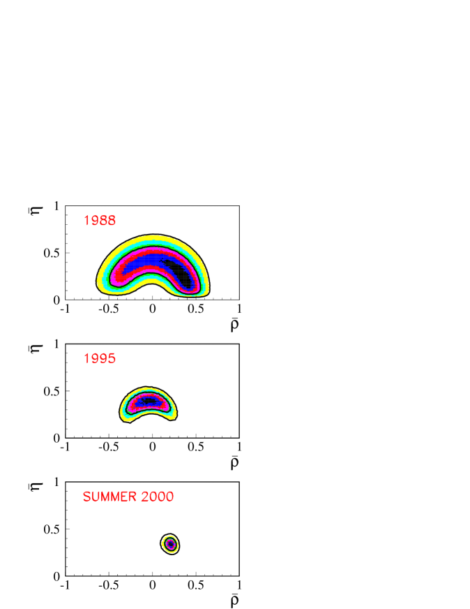
Figure 1: The allowed region for $\overline{\rho}$ and $\overline{\eta}$ (in 1988, 1995 and summer 2000) using the constraints given by the measurements of $\left|V_{ub}\right|/\left|V_{cb}\right|$, $\left|\varepsilon_{K}\right|$, $\Delta m_{d}$ and $\Delta m_{s}$. The contours at 68 $\%$ and 95 $\%$ probability are shown.

Tremendous improvements in the determination of the unitarity triangle parameters have been achieved during the last 10 years as illustrated by the reduction of the selected region in the ($\overline{\rho}-\overline{\eta}$) plane shown in Figure 1. What are the major developments responsible for this success ?

* (a) The continuous and precious work done by the CLEO Collaboration;

* (b) The precise and somehow “unexpected” results obtained by the SLD and LEP Collaborations, which provided the main contribution in the development from the 1995 to 2000 configurations shown in Fig. 1;

* (c) The top quark discovery and the accurate measurement of its mass at the TeVatron;

* (d) The improvements in Lattice QCD calculations;

* (e) The improvements in the theoretical calculations used in extracting $\left|{\rm V}_{cb}\right|$ and $\left|{\rm V}_{ub}\right|$.

In this short note, I summarize the results of Ref. [1], where we determine the parameters of the unitarity triangle using all available recent measurements and theoretical calculations (mainly lattice QCD). Further details can be found in Ref. [2]. I also attempt to demonstrate the robustness of our results.

2 The main actors (Allegro con brio, crescendo continuo)

The central values and the uncertainties for the relevant input parameters used in this analysis are given in Table 1. In the following I give short comments on the determination of the different parameters:

$\left|{\rm V}_{cb}\right|$ – Two methods are used to extract $\left|{\rm V}_{cb}\right|$. The first one makes use of the inclusive semileptonic decays of B-hadrons and the theoretical calculations to extract $\left|{\rm V}_{cb}\right|$ are done in the framework of the Operator-Product-Expansion (OPE). A second method uses the exclusive decays, $\overline{\rm{B}^{0}_{d}}\rightarrow\mbox{D}^{\ast+}\ell^{-}\overline{\nu_{\ell}}$. In this case, the value of $\left|{\rm V}_{cb}\right|$ is obtained by measuring the differential decay rate at maximum mass of the charged lepton-neutrino system, $q^{2}$, in the framework of HQET.

The present exclusive measurements are marginally compatible (the fit probability is 6$\%$). A procedure [3], developed to best combine results which may be in mutual disagreement, has been used to determine the quoted central value for $\left|{\rm V}_{cb}\right|$ shown in Table 1 using inclusive (LEP) and exclusive (LEP and CLEO) measurements. We regard this value as the present world average.

$\left|{\rm V}_{ub}/{\rm V}_{cb}\right|$ – The CLEO collaboration [4] has measured the branching fraction for the decay, $\overline{{\rm B_{d}^{0}}}\rightarrow\rho^{+}\ell^{-}\overline{\nu_{\ell}}$. The value of $\left|{\rm V}_{ub}\right|$ is then deduced using several models. The LEP experiments [5] have measured $Br(b\rightarrow u\ell\bar{\nu}_{l}X)$ with less statistical precision than does CLEO, but with reduced systematic uncertainties. In events with an identified high transverse momentum lepton, they use several kinematical variables, which allow discrimination between b $\rightarrow$ c and b $\rightarrow$ u transitions. Using models based on the OPE, a value for $\left|{\rm V}_{ub}\right|$ is then obtained. These two measurements are shown in Table 1. The uncertainties are uncorrelated between CLEO and LEP results.

$\Delta m_{s}$ – After the addition of recent measurements from the SLD/LEP collaborations, the limit on $\Delta\rm{m}_{s}$, at 95$\%$ C.L. has not increased much compared to last year’s result. But, the sensitivity has improved a lot reaching $\Delta m_{s}=18.0\,ps^{-1}$ [6] (the sensitivity corresponds to the value of $\Delta m_{s}$ ($\Delta m_{s}^{sens}$) at which it is expected that the 95$\%$ limit will be set in 50% of the ideal experiments having the same caracteristics as the real data, if the true value of $\Delta m_{s}$ is much larger than $\Delta m_{s}^{sens}$ )

Non-perturbative QCD parameters – In the framework of lattice QCD, important improvements have been recently achieved in the evaluation of non-perturbative QCD parameters for B hadrons. As a consequence, we use only the most recent values. The central values and the uncertainties given in Table 1 have been evaluated in Ref. [1] and are in good agreement with those given in the three most recent reviews in Ref. [7].

3 The results (Andante allegro)

The region in the ($\overline{\rho},~{}\overline{\eta})$ plane selected by the measurements of $\left|\varepsilon_{K}\right|$, $\left|{\rm V}_{ub}/{\rm V}_{cb}\right|$, $\Delta m_{d}$ and from the limit on $\Delta m_{s}$, is shown at the bottom of Fig. 1. Our fit values for $\overline{\rho}$, $\overline{\eta}$, and the angles are given in Table 2.

Our value, $\sin(2\beta)=0.698\pm 0.066$, is rather precisely determined, compared with the world average, $\sin(2\beta)=0.52\pm 0.22$, measured using $B\rightarrow J/\psi K_{S}$ events. The angle $\gamma$ is known within an accuracy of about 10$\%$. The probability that $\gamma$ is greater than 90^∘ is only 0.03$\%$. This result is mainly due to the improved sensitivity on $\Delta m_{s}$ and is very slightly dependent on the value and on the error assigned to the $\xi$ parameter. ( $\xi={f_{B_{s}}\sqrt{\hat{B_{B_{s}}}}}/{f_{B_{d}}\sqrt{\hat{B_{B_{d}}}}}$ as indicated in Table 1). The central value for the angle $\gamma$ is more than 2$\sigma$ smaller than that obtained in recent fits of rare $B$-meson two-body decays [8] (see for istance [8]-d, where $\gamma=(114^{+24}_{-23})^{\circ}$)

An interesting study consists of removing the theoretical constraint for $\hat{B}_{K}$ in the measurement of $\left|\varepsilon_{K}\right|$. The corresponding selected region in the ($\overline{\rho},~{}\overline{\eta})$ plane is shown in Figure 2. In Figure 2 the regions (at 68% and 95% probability) selected by the measurement of $\left|\varepsilon_{K}\right|$ alone are also drawn. This comparison shows that the Standard Model picture of CP violation in the $K$ system and of $B$ decays and oscillations is consistent. This constitutes already a test of compatibility between the measurements of the sides and of the angles of the CKM triangle. This can be quantified by comparing the value, $\hat{B}_{K}=0.87\pm 0.06\pm 0.13$, obtained from lattice-QCD calculations, with the one extracted by using constraints from $b$-physics alone, $\hat{B}_{K}=0.90^{+0.30}_{-0.14}$. In the same figure, we also compare the allowed regions in the ($\overline{\rho},~{}\overline{\eta})$ plane with those selected by the measurement of $\sin(2\,\beta)$ using $J/\psi K_{S}$ events.
It is informative to remove other theoretical or experimental constraints from a fit (as $\hat{B}_{K}$ in the previous example). This illustrates the effectiveness of a constraint and gives a most like value of a parameter within the Standard Model. The most significant results we find are :

$$f_{B_{d}}\sqrt{\hat{B}_{B_{d}}}=(230\pm 12)~{}\rm{MeV}\,,\quad\Delta m_{s}=(16.3\pm 3.4)ps^{-1}$$ (1)

4 Stability Tests (Adagio….. con calma)

To determine the robustness of our results, we investigate how the quoted accuracies on the unitarity triangle parameters change if: (a) the errors on the input parameters are changed, or (b) a different statistical method is used to obtain the results.

(a) – It is a basic exercise to verify how the accuracy quoted on final results depends on the assumed errors for the different input parameters. A similar analysis has been already presented in [2]. As shown in Table 2, all the flat theoretical errors, as well as the error on $\left|{\rm V}_{cb}\right|$, are multiplied by a factor of 2. Thus, the assumed error on $\left|{\rm V}_{cb}\right|$ is ($\pm 3.8\times 10^{-3}$); on $\hat{B}_{K}$, it is ($\pm$ 0.06(Gaussian) $\pm$ 0.26(flat)). The main conclusion of this study is that, even in this extreme case, the unitarity triangle parameters are determined with uncertainties which increase by about a factor of 1.6.

2) A comparison between our results (using a Bayesian approach, see Ref. [1] for more details) and those obtained using the “scanning method” (adopted by the Babar Collaboration), has been done. To do this comparison, the same central values and errors for the parameters have been used in the two cases. When a parameter is scanned, in the “scanning approach”, a flat distribution corresponding to the scanning range is used in our approach. These parameters are those given in  [9]. The “95$\%$ C.L.” contours obtained with the two methods are compared in Fig. 3. The main conclusion is that, when the same input parameters are used, very similar results are obtained using the two methods. We therefore do not believe that our method yields “optimistic” results.

5 Conclusions (Finale con brio)

The determination of the unitarity triangle parameters has already entered in a mature age, the age of precision tests. I have illustrated the impressive improvements on the determination of the two sides of the unitarity triangle using only B decays and oscillations. Our results are shown to be robust and stable against changes in the uncertainties of the input parameters and against the statistical method used to obtain them.

The selected region in the ($\overline{\rho}$-$\overline{\eta}$) plane is compatible with the measurement of CP violation in the Kaon system. Similar tests are expected soon from the direct measurement of sin(2$\beta$) at B-Factories and future hadron machines.

Table 1: Values of the quantities entering into the expressions of $\left|\varepsilon_{K}\right|$, $\left|{\rm V}_{ub}/{\rm V}_{cb}\right|$, $\Delta m_{d}$ and $\Delta m_{s}$. The Gaussian and the flat part of the error are given explicitly.

Parameters	Std. Result	Theo. x 2 ,  $\left|{\rm V}_{cb}\right|$ x 2	Maximal Increase
$\overline{\rho}$	0.224 $\pm$ 0.038	$\pm$ 0.064	$\sim$1.7
$\overline{\eta}$	0.317 $\pm$ 0.040	$\pm$ 0.065	$\sim$1.6
sin2$\beta$	0.698 $\pm$ 0.066	${}^{+0.086}_{-0.101}$	$\sim$1.4
sin2$\alpha$	-0.42 $\pm$ 0.23	$\pm$ 0.37	$\sim$1.6
$\gamma$	(54.8 $\pm$ 6.2)o	$(\pm$ 10.0)o	$\sim$1.6

Table 2: Stability tests. Variation of the error on some unitarity triangle parameters obtained by multiplying the flat part of the theoretical error by a factor 2 as well as the error on $\left|{\rm V}_{cb}\right|$ by the same factor.

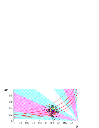
Figure 2: The allowed regions (at 68%, 95%, 99% and 99.9% probability) for $\overline{\rho}$ and $\overline{\eta}$ using the constraints given by the measurements of $\left|V_{ub}\right|/\left|V_{cb}\right|$, $\Delta m_{d}$ and $\Delta m_{s}$. The constraint due to $\left|\varepsilon_{K}\right|$ is not included. The regions (at 68% and 95% probability) selected by the measurements of $\left|\varepsilon_{K}\right|$ (continuous (1$\sigma$) and dotted (2$\sigma$) curves) and $\sin(2\,\beta)$ (darker (1$\sigma$) and clearer (2$\sigma$) zones) are shown. For $\sin(2\,\beta)$ the two solutions are displayed.

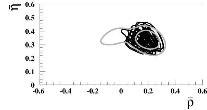
Figure 3: The contour corresponding to 95$\%$ probability, using our approach (continous contour), is compared with the envelope of 95$\%$ C.L. ellipses, obtained using the 95$\%$ C.L. “scanning method”. In the former case, the 68$\%$ contour is also shown. The parameters used in this study are those given in Ref. [9]. The allowed region in the ($\overline{\rho}$-$\overline{\eta}$) plane is larger than the one shown at the bottom of Fig. 1 because input parameters correspond,respectively, to the current knowledge at the beginning of 1998 and summer 2000

References

- [1] M. Ciuchini, G. D’Agostini, E. Franco, V. Lubicz, G. Martinelli, F. Parodi, P. Roudeau, A. Stocchi hep-ph/0012308 submitted to JHEP
- [2] M. Ciuchini et al., Z. Phys. C68 (1995) 239; P. Paganini et al., Phys. Scripta V. 58 (1998) 556; F. Parodi et al., Nuovo Cim. 112A (1999) 833; F. Caravaglios et al., hep-ph/0002171, talk at “BCP 99”, Taipei, Taiwan Dec. 3-7 1999; M. Ciuchini et al., Nucl. Phys. B573 (2000) 201.
- [3] G. D’Agostini, CERN-EP/99-139 and hep-ex/9910036.
- [4] B.H. Behrens et al., (CLEO Coll.), Phys. Rev. D61 (2000) 052001.
- [5] LEP WG, http://battagl.home.cern.ch/battagl/vub/vub.html.
- [6] A. Stocchi, hep-ph/0010222, talk at XXXth ICHEP 27 Jul.-2 Aug. 2000, Osaka, Japan.; F. Palla, these proceedings.
- [7] R.D. Kenway, hep-ph/0010219 plenary talk at XXXth ICHEP 27 Jul.-2 Aug. 2000, Osaka, Japan; V. Lubicz, hep-ph/00101711, talk at the XXth Physics in Collision, Jun. 29-Jul. 1 2000, Lisbon, Portugal; C. Bernard, hep-lat/0011064 plenary talk at Lattice 2000.
- [8] a) M. Gronau, J.L. Rosner, Phys. Rev. D61 (2000) 073008; b) X.G. He et al., Phys. Rev. Lett. 83 (1999) 1100; c) W.S. Hou, K.-C. Yang, hep-ph/9908202; d) W.S. Hou et al., hep-ex/9910014; e) H.Y. Cheng, K.C. Yang, hep-ph/9910291; f) B. Dutta, S. Oh, hep-ph/9911263; g) Y.F. Zhou et al., hep-ph/0006225.
- [9] S. Plaszczynski, M.-H. Schune, hep-ph/9911280.
- [10] F. Abe et al., (CDF Coll.), Phys. Rev. Lett. 74 (1995) 2626; S. Abachi et al., (D0 Coll.), Phys. Rev. Lett. 74 (1995) 2632.