The $\eta^{\prime}g^{*}g^{*}$ Vertex with Arbitrary Gluon Virtualities
in the Perturbative QCD Hard Scattering Approach

Abstract

We study the $\eta^{\prime}g^{*}g^{*}$ vertex for arbitrary gluon virtualities in the time-like and space-like regions, using the perturbative QCD hard scattering approach and an input wave-function of the $\eta^{\prime}$-meson consistent with the measured $\eta^{\prime}\gamma^{*}\gamma$ transition form factor. The contribution of the gluonic content of the $\eta^{\prime}$-meson is taken into account, enhancing the form factor over the entire virtuality considered. However, data on the electromagnetic transition form factor of the $\eta^{\prime}$-meson is not sufficient to quantify the gluonic enhancement. We also study the effect of the transverse momenta of the partons in the $\eta^{\prime}$-meson on the $\eta^{\prime}g^{*}g^{*}$ vertex, using the modified hard scattering approach based on Sudakov formalism, and contrast the results with the ones in the standard hard scattering approach in which such effects are neglected. Analytic expressions for the $\eta^{\prime}g^{*}g^{*}$ vertex are presented in limiting kinematic regions and parametrizations are given satisfying the QCD anomaly, for real gluons, and perturbative QCD behavior for large gluon virtualities, in both the time-like and space-like regions. Our results have implications for the inclusive decay $B\to\eta^{\prime}X$ and exclusive decays, such as $B\to\eta^{\prime}(K,K^{*})$, and in hadronic production processes $N+N(\bar{N})\to\eta^{\prime}X$.

I Introduction

The vertex involving the coupling of two gluons and $\eta^{\prime}$-meson $F_{\eta^{\prime}g^{*}g^{*}}(q_{1}^{2},q_{2}^{2},m_{\eta^{\prime}}^{2})$ (here, $q_{1}^{2}$ and $q_{2}^{2}$ represent the virtualities of the two gluons) enters in a number of production and decay processes. For example, the inclusive decays $B\to\eta^{\prime}X_{s}$ cleo-etap-incl and exclusive decays $B\to\eta^{\prime}K$ cleo-etap-excl ; babar-etap , involve, apart from the matrix elements of the four-quark operators, the transitions $b\to sg^{*}$, followed by $g^{*}\to\eta^{\prime}g$ TFF-3 ; TFF-2 , $b\to sgg$ followed by $gg\to\eta^{\prime}$ ACGK98 , as well as the transitions $g^{*}g^{*}\to\eta^{\prime}$ and $g^{*}g\to\eta^{\prime}$ TFF-1 . Thus, a reliable determination of the vertex function (which can also be termed as the gluonic transition form factor) $F_{\eta^{\prime}g^{*}g^{*}}(q_{1}^{2},q_{2}^{2},m_{\eta^{\prime}}^{2})$ is an essential input in a quantitative understanding of these and related decays. Apart from the mentioned $B$-decays, the $\eta^{\prime}g^{*}g^{(*)}$ vertex plays a role in a large number of processes, among them the radiative decay $J/\psi\to\eta^{\prime}\gamma$ and the hadronic production processes $N+N(\bar{N})\to\eta^{\prime}+X$, where $N$ is a nucleon. The QCD axial anomaly anomaly , responsible for the bulk of the $\eta^{\prime}$-meson mass, normalizes the vertex function on the gluon mass-shell, yielding $F_{\eta^{\prime}g^{*}g^{*}}(0,0,m_{\eta^{\prime}}^{2})$. The question that still remains concerns the determination of the vertex for arbitrary time-like and space-like virtualities, $q_{i}^{2}$; $i=1,2$. A related aspect is to understand the relation between the $\eta^{\prime}g^{*}g^{*}$ vertex and the wave-function of the $\eta^{\prime}$-meson. Stated differently, issues such as the transverse momenta of the partons in the $\eta^{\prime}$-meson and their impact on the $\eta^{\prime}g^{*}g^{*}$ vertex have to be studied quantitatively.

While information on the $\eta^{\prime}g^{*}g^{*}$ vertex is at present both indirect and scarce, its electromagnetic counterpart involving the coupling of two photons and the $\eta^{\prime}$-meson, $F_{\eta^{\prime}\gamma^{*}\gamma}$, more generally the meson-photon transition form factor, has been the subject of intense theoretical and experimental activity. In particular, the hard scattering approach to transition form factors, developed by Brodsky and Lepage BL , has been extensively used in studying perturbative QCD effects and in making detailed comparison with data BL-Review . A variation of the hard scattering approach, in which transverse degrees of freedom are included in the form of Sudakov effects in transition form factors Collins ; BS89 , has also been employed in data analyses. It has been argued BS89 ; Ong ; JKR96 that the Sudakov effects improve the applicability of perturbative QCD methods down to moderate values of $Q^{2}$ and give a better account of data on meson-photon transitions eta'-gamma . For a critical review and comparison of the standard (Brodsky-Lepage) and modified (mHSA) hard scattering approaches, see Refs. MR97 ; Stefanis99 . We note that either of these approaches combined with data constrains the input wave-function for the quark-antiquark part of the $\eta^{\prime}$-meson. However, the gluonic part of the $\eta^{\prime}$-meson wave-function is not directly measured in these experiments and will be better constrained in future experiments sensitive to the $\eta^{\prime}g^{*}g^{*}$ vertex.

A closely related issue is that of the $\eta-\eta^{\prime}$ mixing. There exist good theoretical Leutwyler and phenomenological FK98 reasons to suspect that the frequently assumed pattern of the decay constants $f_{P}^{k}$, defined by the equations

$$\langle 0|J_{\mu 5}^{k}|P(p)\rangle=if_{P}^{k}p_{\mu},\qquad(k=8,1;\quad P=\eta,\eta^{\prime}),$$ (1)

where $J_{\mu 5}^{8}$ and $J_{\mu 5}^{1}$ denotes the SU(3)_F octet and singlet axial-vector currents, respectively, do not follow the pattern of state mixing. Defining the decay constants as Leutwyler

$$f_{\eta}^{8}=f_{8}\cos\theta_{8},\quad f_{\eta}^{1}=-f_{1}\sin\theta_{1},$$

$$f_{\eta^{\prime}}^{8}=f_{8}\sin\theta_{8},\quad f_{\eta^{\prime}}^{1}=f_{1}\cos\theta_{1},$$ (2)

the angles $\theta_{1}$ and $\theta_{8}$ are found to differ considerably due to non-negligible SU(3)_F-breaking effects Leutwyler ; FK98 . In contrast, it is natural to expect that the state mixing is determined essentially by a single angle, as the state $\eta_{c}$ is far too heavy to be significant in the state-mixing in the $\eta-\eta^{\prime}$ complex. A growing consensus is now emerging in favor of the two mixing-angle scheme of Leutwyler Leutwyler for the decay constants in Eq. (2) FK98 ; FKS98 . To be precise, we shall use the state-mixing scheme of Feldmann, Kroll and Stech FKS98 , which is consistent with the two mixing-angle scheme of Ref. Leutwyler in the current-mixing basis.

Based on the foregoing discussion, it is natural to use the hard scattering approach to study the $\eta^{\prime}g^{*}g^{*}$ vertex, incorporating the information on the wave-function and the mixing parameters entering in the $\eta-\eta^{\prime}$ complex from existing data involving the electromagnetic transitions. A first step in this direction was undertaken recently by Muta and Yang Muta . They derived the $\eta^{\prime}g^{*}g$ vertex in the time-like region in terms of the quark-antiquark and gluonic parts of the $\eta^{\prime}$-meson wave-function, taking into account the evolution equations obeyed by these partonic components Ohrndorf:1981uz . In this paper, we also address the same issue along very similar lines. We first rederive the $\eta^{\prime}g^{*}g$ vertex, pointing out the agreement and differences between our results and the ones in Ref. Muta . The latter have to do with the derivation of the leading order perturbative contribution to the gluonic part of the $\eta^{\prime}g^{*}g$ vertex, and the use by Muta and Yang Muta of the anomalous dimensions derived in Ref. Ohrndorf:1981uz in the evolution of the wave-functions. For the anomalous dimensions, we use now, correcting a similar mistake in the earlier version of this paper, the results derived in Refs. Shifman:1981dk ; Baier:1981pm , which are at variance with the ones given in Ref. Ohrndorf:1981uz , but which have been recently confirmed by Belitsky and Müller Belitsky . Making use of the $\eta^{\prime}\gamma^{*}\gamma$ data to constrain the $\eta^{\prime}$-meson wave-function parameters, we find that the gluonic contribution in the $\eta^{\prime}$-meson is very significant. We then extend our analysis to the case when both the gluons are virtual, having either the time-like or space-like virtualities. We also present a number of results on the vertex function $F_{\eta^{\prime}g^{*}g^{*}}(q_{1}^{2},q_{2}^{2},m_{\eta^{\prime}}^{2})$ in the asymptotic region, which have not been presented earlier to the best of our knowledge, and are of use in future theoretical analysis, in particular in the $B\to\eta^{\prime}X$ and $B\to\eta^{\prime}(K,K^{*})$ transitions. We study the effects of the transverse momentum distribution involving the constituents of the $\eta^{\prime}$-meson and take into account soft-gluon emission from the constituent partons by including the QCD Sudakov factor, following techniques en vogue in studies of the electromagnetic and transition form factors of the mesons JKR96 ; JK93 ; Stefanis99 . We show the improvements in the $\eta^{\prime}g^{*}g^{(*)}$ vertex function due to the inclusion of the transverse-momentum and Sudakov effects, which are particularly marked in the space-like region, improving the applicability of the hard scattering approach to low values of $Q^{2}$. These effects have a bearing on the hard scattering approach to exclusive non-leptonic decays BBNS99 ; the importance of the transverse-momentum and Sudakov effects in the decays $B\to\pi\pi$ and $B\to K\pi$ has also been recently emphasized in Ref. KL00 . Finally, we also derive approximate formulae for the $\eta^{\prime}g^{*}g^{(*)}$ vertex, which satisfy the axial-vector anomaly result for on-shell gluons and the asymptotic behavior in the large-$Q^{2}$ domain, determined by perturbative QCD.

This paper is organized as follows: In section II, we specify the $\eta-\eta^{\prime}$ mixing formalism and the evolution equations for the $q\bar{q}$ and gluonic wave-functions of the $\eta^{\prime}$-meson. In section III, the $q\bar{q}$ contribution to the off-shell $\eta^{\prime}g^{*}g^{*}$ vertex is worked out in the hard scattering approach. The corresponding contributions from the gluons are presented in section IV. In section V, we implement the transverse-momentum effects and derive the Sudakov-improved $\eta^{\prime}g^{*}g^{*}$ vertex. Numerical results are presented in section VI, where we also show comparison with existing results. In section VII, we give simple formulae for the $\eta^{\prime}g^{*}g^{*}$ vertex, which interpolate between the well-known limiting cases. Our main results are summarized in section VIII. Appendix A contains the solution of the evolution equations for the wave functions $\phi^{(q)}(x,Q)$ and $\phi^{(g)}(x,Q)$, and the function $J(\omega,\eta)$ introduced in the derivation of the $\eta^{\prime}g^{*}g^{*}$ vertex in section III is given in Appendix B.

II $\eta^{\prime}$-Meson Wave-Function

The $\eta^{\prime}$-meson is not a flavor-octet meson state and, hence, in addition to the usual quark content the $\eta^{\prime}$-meson wave-function has a gluonic admixture. In principle, there also exist a $\bar{c}c$ component in the $\eta^{\prime}$-meson wave-function, but it has been estimated to be rather small in well-founded theoretical frameworks ACGK98 ; AG97 ; FKS98 , and hence ignored. We take the parton Fock-state decomposition of the $\eta^{\prime}$-meson wave-function as follows:

$$|\eta^{\prime}>\,=\sin\phi\,|\eta^{\prime}_{q}>+\cos\phi\,|\eta^{\prime}_{s}>+\,|\eta^{\prime}_{g}>,$$ (3)

where the SU(3)_F symmetry among the light $u$, $d$ and $s$ quarks is assumed so that $|\eta^{\prime}_{q}>\,\sim|\bar{u}u+\bar{d}d>/\sqrt{2}$ and $|\eta^{\prime}_{s}>\,\sim|\bar{s}s>$ are the quark Fock states and $\phi$ is the mixing angle; $|\eta^{\prime}_{g}>\,\sim|gg>$ is the two-gluon Fock state. In Refs. Ohrndorf:1981uz ; Shifman:1981dk ; Baier:1981pm the eigenfunctions of the mixing quark $|\bar{q}q>$ and gluonic $|gg>$ state:

$$\Psi = C\left[\phi^{(q)}(x,Q)+\phi^{(g)}(x,Q)\right],$$ (4)

$$C = \sqrt{2}\,f_{q}\sin\phi+f_{s}\cos\phi,$$ (5)

where $f_{q}$ and $f_{s}$ are the decay constants of $|{\eta^{\prime}}_{q}>$ and $|{\eta^{\prime}}_{s}>$, have been calculated by solving the evolution equations. The result for the quark and gluonic components is presented as infinite series of the Gegenbauer polynomials of the indices $3/2$ and $5/2$ GR and can be found in Appendix A. Previous analyses show that it is a good approximation to consider only a few first terms in the expansion of the quark and gluonic wave-function. Here, we shall keep the leading two terms in the expansion for $\phi^{(q)}(x,Q)$, and keep only the first term for $\phi^{(g)}(x,Q)$:

$$\phi^{(q)}(x,Q)=6x\bar{x}\left\{1+\left[6B^{(q)}_{2}\left(\frac{\alpha_{s}(Q^{2})}{\alpha_{s}(\mu_{0}^{2})}\right)^{\frac{48}{81}}-\frac{B^{(g)}_{2}}{15}\left(\frac{\alpha_{s}(Q^{2})}{\alpha_{s}(\mu_{0}^{2})}\right)^{\frac{101}{81}}\right](1-5x\bar{x})+\cdots\right\},$$ (6)

$$\phi^{(g)}(x,Q)=x\bar{x}(x-\bar{x})\left[16B^{(q)}_{2}\left(\frac{\alpha_{s}(Q^{2})}{\alpha_{s}(\mu_{0}^{2})}\right)^{\frac{48}{81}}+5B^{(g)}_{2}\left(\frac{\alpha_{s}(Q^{2})}{\alpha_{s}(\mu_{0}^{2})}\right)^{\frac{101}{81}}\right]+\cdots,$$ (7)

where $x$ and $\bar{x}=1-x$ are the energy fractions of two partons inside the $\eta^{\prime}$-meson, $Q^{2}>0$ is the energy scale parameter, and $\mu_{0}\simeq 0.5$ GeV is the typical hadronic energy scale below which no perturbative evolution takes place.

Figure 1: Leading Feynman diagrams contributing to the quark part of the $\eta^{\prime}g^{*}g^{*}$ vertex.

It is seen that in the limit $Q^{2}\to\infty$ the quark wave-function (6) turns to its asymptotic form $\phi_{\rm as}(x)=6x\bar{x}$ (the same asymptotic behavior as the pion wave-function BL due to its quark content), while the gluonic wave-function (7) vanishes in this limit, $\phi^{(g)}_{\rm as}(x)=0$. The coefficients of the expansion of the wave-functions (6) and (7) are calculated by using perturbation theory and include the effective QCD coupling $\alpha_{s}(Q^{2})$, which in the next-to-leading logarithmic approximation is given by PDG

$$\alpha_{s}(Q^{2})=\frac{4\pi}{\beta_{0}\ln(Q^{2}/\Lambda^{2})}\left[1-\frac{2\beta_{1}}{\beta_{0}^{2}}\,\frac{\ln\ln(Q^{2}/\Lambda^{2})}{\ln(Q^{2}/\Lambda^{2})}\right],$$ (8)

where $\beta_{0}=11-2n_{f}/3$, $\beta_{1}=51-19n_{f}/3$, $\Lambda=\Lambda_{\rm QCD}$ is the QCD scale parameter, and $n_{f}$ is the number of quarks with masses less than the energy scale $Q$. In the energy region $\bar{m}_{c}<Q<\bar{m}_{b}$, where $\bar{m}_{c}=1.3\pm 0.3$ GeV and $\bar{m}_{b}=4.3\pm 0.2$ GeV are the charm and bottom $\overline{\rm MS}$ quark masses, respectively, we will use the value of the dimensional parameter $\Lambda^{(4)}_{\overline{\rm MS}}=280$ MeV corresponding to four active quark flavors PDG . The requirement that the effective QCD coupling is continuous at the flavor thresholds leads to a change of $\Lambda$ in the threshold energy regions where $n_{f}$ changes. This implies that for $Q<\bar{m}_{c}$, the value of $\Lambda$ is rescaled, yielding $\Lambda^{(3)}_{\overline{\rm MS}}=333$ MeV.

III Quark-Antiquark Contribution to the $\eta^{\prime}g^{*}g^{*}$ Vertex

The diagrams depicting the quark-antiquark content of the $\eta^{\prime}g^{*}g^{*}$ vertex (or transition amplitude) are shown in Fig. 1. The invariant amplitude corresponding to the quark contribution to the $\eta^{\prime}g^{*}g^{*}$ vertex in the momentum space can be defined as:

$${\cal M}^{(q)}=\frac{C}{4N_{c}}\int\limits_{0}^{1}dx\,\phi^{(q)}(x,Q)\,{\rm Sp}[\gamma_{5}(\hbox to0.0pt{/\hss}P-m_{\eta^{\prime}})T^{(q)}_{\rm H}],$$ (9)

where $P_{\mu}$ and $m_{\eta^{\prime}}$ are the four-momentum and the mass of the $\eta^{\prime}$-meson, respectively, $\hbox to0.0pt{/\hss}P=P_{\mu}\gamma^{\mu}$, $\gamma_{\mu}$ and $\gamma_{5}$ are the Dirac $\gamma$-matrices, and $T^{(q)}_{\rm H}$ is the hard amplitude connected with the effective quark-antiquark-two-gluon vertex by the following relation:

$$T^{(q)}_{\rm H}=\delta_{\alpha\beta}\,V^{\beta\alpha;ab}_{\mu\nu}(xP,\bar{x}P,-q_{1},-q_{2})\,\varepsilon^{a*}_{\mu}\varepsilon^{b*}_{\nu},$$ (10)

where the summation over the quarks’ colors $\alpha$ and $\beta$ allows to get a color-singlet meson state and $x$ and $\bar{x}$ have been defined earlier in Sec. II. In the leading order in the strong coupling $\alpha_{s}$, the effective quark-antiquark-gluon-gluon vertex is presented in Fig. 2 and has the form:

$$V^{\beta\alpha;ab}_{\mu\nu}(p_{1},p_{2},q_{1},q_{2})=-4\pi\alpha_{s}\,\bigg{\{}\frac{i\,f_{abc}(t_{c})_{\beta\alpha}}{(q_{1}+q_{2})^{2}+i\epsilon}\qquad$$ (11)

$$\times\left[(\hbox to0.0pt{/\hss}q_{1}-\hbox to0.0pt{/\hss}q_{2})g_{\mu\nu}+(q_{1}+2q_{2})_{\mu}\gamma_{\nu}-(2q_{1}+q_{2})_{\nu}\gamma_{\mu}\right]$$

$$+\left(t_{b}t_{a}\right)_{\beta\alpha}\frac{\gamma_{\nu}(\hbox to0.0pt{/\hss}p_{1}+\hbox to0.0pt{/\hss}q_{1}+m_{q})\gamma_{\mu}}{(p_{1}+q_{1})^{2}-m_{q}^{2}+i\epsilon}$$

$$+\left(t_{a}t_{b}\right)_{\beta\alpha}\frac{\gamma_{\mu}(\hbox to0.0pt{/\hss}p_{1}+\hbox to0.0pt{/\hss}q_{2}+m_{q})\gamma_{\nu}}{(p_{1}+q_{2})^{2}-m_{q}^{2}+i\epsilon}\bigg{\}},$$

where $t_{a}$ ($a=1,\ldots,N_{c}^{2}-1$) are the generators of the color SU($N_{c}$) group, $f_{abc}$ are its antisymmetric structure constants, $g_{\mu\nu}={\rm diag}(1,-1,-1,-1)$ is the metric tensor, $m_{q}$ is the quark mass, and $\hbox to0.0pt{/\hss}q=q_{\mu}\gamma^{\mu}$. In the calculation of the amplitude, we have neglected all the quark masses $m_{q}$ as they are much smaller than the energy scale parameter $Q$.

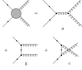
Figure 2: The effective quark-antiquark-gluon-gluon vertex and leading order contributions.

Defining the quark contribution to the $\eta^{\prime}g^{*}g^{*}$ vertex $F^{(q)}_{\eta^{\prime}g^{*}g^{*}}$ as:

$${\cal M}^{(q)}\equiv-i\,F^{(q)}_{\eta^{\prime}g^{*}g^{*}}(q_{1}^{2},q_{2}^{2},m_{\eta^{\prime}}^{2})\,\delta_{ab}\,\varepsilon^{\mu\nu\rho\sigma}\,\varepsilon^{a*}_{\mu}\varepsilon^{b*}_{\nu}q_{1\rho}q_{2\sigma},$$ (12)

the result of the calculation is:

$$F^{(q)}_{\eta^{\prime}g^{*}g^{*}}(q_{1}^{2},q_{2}^{2},m_{\eta^{\prime}}^{2})=4\pi\alpha_{s}(Q^{2})\,\frac{C}{2N_{c}}\int\limits_{0}^{1}dx\,\phi^{(q)}(x,Q)$$

$$\times\left[\frac{1}{xq_{1}^{2}+\bar{x}q_{2}^{2}-x\bar{x}m_{\eta^{\prime}}^{2}+i\epsilon}+(x\leftrightarrow\bar{x})\right].$$ (13)

Note that the quark wave-function of the $\eta^{\prime}$-meson satisfies the symmetry condition $\phi^{(q)}(x,Q)=\phi^{(q)}(\bar{x},Q)$ Ohrndorf:1981uz ; Shifman:1981dk ; Baier:1981pm . When one of the gluons is on the mass shell, for example $q_{2}^{2}=0$, the quark part of the $\eta^{\prime}g^{*}g^{*}$ vertex, $F^{(q)}_{\eta^{\prime}g^{*}g^{*}}(q_{1}^{2},0,m_{\eta^{\prime}}^{2})$, agrees with the one presented in Ref. Muta .

In the case when both virtualities of the gluons are of the same signs (space-like $q_{1}^{2}<0$, $q_{2}^{2}<0$ or time-like $q_{1}^{2}>0$, $q_{2}^{2}>0$) the quark contribution to the $\eta^{\prime}g^{*}g^{*}$ vertex can be presented in the form:

$$F^{(q)}_{\eta^{\prime}g^{*}g^{*}}(q^{2},\omega,\eta) = \frac{4\pi\alpha_{s}(Q^{2})}{q^{2}}\,\frac{2C}{N_{c}}$$

$$\times \int\limits_{0}^{1}\frac{(1-2x\bar{x}\eta)\,\phi^{(q)}(x,Q)\,dx}{(1-2x\bar{x}\eta)^{2}-\omega^{2}(x-\bar{x})^{2}+i\epsilon},$$

where $q^{2}=q_{1}^{2}+q_{2}^{2}$ is the total gluon virtuality, $\omega=(q_{1}^{2}-q_{2}^{2})/q^{2}$ is the asymmetry parameter having the values in the domain $-1\leq\omega\leq 1$, and $\eta=m_{\eta^{\prime}}^{2}/q^{2}$ is the scaled $\eta^{\prime}$-meson mass squared. As a typical mass scale $Q$ which defines the value of the strong coupling $\alpha_{s}(Q^{2})$, it is natural to consider the absolute value of the total virtuality $Q^{2}=|q^{2}|$. The quark contribution, $F^{(q)}_{\eta^{\prime}g^{*}g^{*}}$, corresponding to keeping the first two terms in the quark wave-function (6) is:

$$F^{(q)}_{\eta^{\prime}g^{*}g^{*}}(Q^{2},\omega,\eta)=F^{(q)}_{0}(Q^{2},\omega,\eta)+F^{(q)}_{2}(Q^{2},\omega,\eta)$$

$$=\frac{4\pi\alpha_{s}(Q^{2})}{m_{\eta^{\prime}}^{2}}\,\frac{6C}{N_{c}}\left\{{\rm G}^{(q)}_{0}(\omega,\eta)+{\rm G}^{(q)}_{2}(\omega,\eta)\vphantom{\left(\frac{\alpha_{s}(Q^{2})}{\alpha_{s}(\mu_{0}^{2})}\right)^{\frac{48}{81}}}\right.$$ (15)

$$\times\left.\left[6B^{(q)}_{2}\left(\frac{\alpha_{s}(Q^{2})}{\alpha_{s}(\mu_{0}^{2})}\right)^{\frac{48}{81}}-\frac{B^{(g)}_{2}}{15}\left(\frac{\alpha_{s}(Q^{2})}{\alpha_{s}(\mu_{0}^{2})}\right)^{\frac{101}{81}}\right]\right\},$$

where the functions ${\rm G}^{(q)}_{0}$ and ${\rm G}^{(q)}_{2}$ are:

$${\rm G}^{(q)}_{0}(\omega,\eta)=-1+\frac{\omega}{2\eta}\,\ln\left|\frac{1+\omega}{1-\omega}\right|+\left[1-\frac{\omega^{2}}{\eta}\right]{\rm J}(\omega,\eta),$$ (16)

$${\rm G}^{(q)}_{2}(\omega,\eta) = -\frac{1}{6}+\frac{5}{2\eta}-\frac{5\omega^{2}}{\eta^{2}}$$

$$+ \frac{\omega}{2\eta}\left[1-\frac{5}{\eta}+\frac{5\omega^{2}}{\eta^{2}}\right]\ln\left|\frac{1+\omega}{1-\omega}\right|$$

$$+ \left[1-\frac{5+7\omega^{2}}{2\eta}+\frac{10\omega^{2}}{\eta^{2}}-\frac{5\omega^{4}}{\eta^{3}}\right]{\rm J}(\omega,\eta).$$

Notice that ${\rm G}^{(q)}_{i}(\omega,\eta)$ ($i=0,2$) are symmetric in their first argument under the interchange $\omega\to-\omega$: ${\rm G}^{(q)}_{i}(-\omega,\eta)={\rm G}^{(q)}_{i}(\omega,\eta)$. The function ${\rm J}(\omega,\eta)$ is defined and analyzed in Appendix B.

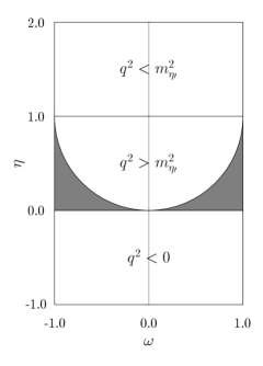
Figure 3: The $\omega-\eta$ parameter plane of the $\eta^{\prime}g^{*}g^{*}$ vertex. The regions over which the vertex has an imaginary part are indicated by the gray color.

In the space-like region of the gluon virtualities, where $\eta<0$, the $\eta^{\prime}g^{*}g^{*}$ vertex is real as in this case the quark propagator does not have poles which is clearly seen from Eq. (III). In the time-like region of the virtualities, for those values of the asymmetry $\omega$ and the relative $\eta^{\prime}$-meson mass squared $\eta$ for which the inequality $\omega^{2}+(1-\eta)^{2}>1$ is satisfied (Fig. 3), an imaginary part in the vertex function appears due to the function $J(\omega,\eta)$ as the result of the $i\epsilon$ prescription of the quark propagator (see Eq. (13)). Notice that if one of the gluons is on the mass shell, for example the second one, $q_{2}^{2}=0$, the imaginary part is nonzero for any value of the other virtuality in the region $q_{1}^{2}>m_{\eta^{\prime}}^{2}$. For large gluon virtualities the imaginary part of the vertex becomes large due to the linear dependence on $q^{2}$ of the leading contribution, ${\rm Im}\,F^{(q)}_{0}\sim q^{2}$, and the cubic dependence of the next-to-leading contribution, ${\rm Im}\,F^{(q)}_{2}\sim(q^{2})^{3}$. This rapid increase of the imaginary part of the $\eta^{\prime}g^{*}g^{*}$ vertex function with the total gluon virtuality seems unphysical and the natural prescription in the Brodsky-Lepage approach is to drop the imaginary part. The physical interpretation of this procedure will be discussed in Sec. V. In the following, we shall drop the imaginary part of the $\eta^{\prime}g^{*}g^{*}$ vertex in the Brodsky-Lepage approach.

Figure 4: The functions $f_{0}(\omega)$, $f_{2}(\omega)$, and $g_{2}(\omega)$ describing the large $Q^{2}$ asymptotics of the $\eta^{\prime}g^{*}g^{*}$ vertex, with the two gluon virtualities having same signs.

It is useful to find the asymptotics of the quark contribution to the $\eta^{\prime}g^{*}g^{*}$ vertex at large $Q^{2}$ ($|\eta|\ll 1$ or equivalently $Q^{2}\gg m_{\eta^{\prime}}^{2}$) for arbitrary values of the asymmetry parameter $\omega$. As in the case of the $\pi\gamma^{*}\gamma^{*}$ transition form factor the function describing the $\eta^{\prime}g^{*}g^{*}$ vertex decreases like $\sim 1/Q^{2}$:

$$F^{(q)}_{\eta^{\prime}g^{*}g^{*}}(Q^{2},\omega,0)\simeq F^{(q)}_{0}(Q^{2},\omega,0)+F^{(q)}_{2}(Q^{2},\omega,0)$$

$$=\frac{4\pi\alpha_{s}(Q^{2})}{Q^{2}}\,\frac{3C}{N_{c}}\,\left\{f_{0}(\omega)+f_{2}(\omega)\vphantom{\left(\frac{\alpha_{s}(Q^{2})}{\alpha_{s}(\mu_{0}^{2})}\right)^{\frac{48}{81}}}\right.$$ (18)

$$\times\left.\left[6B^{(q)}_{2}\left(\frac{\alpha_{s}(Q^{2})}{\alpha_{s}(\mu_{0}^{2})}\right)^{\frac{48}{81}}-\frac{B^{(g)}_{2}}{15}\left(\frac{\alpha_{s}(Q^{2})}{\alpha_{s}(\mu_{0}^{2})}\right)^{\frac{101}{81}}\right]\right\},$$

where the two functions of the asymmetry parameter introduced above are defined as follows:

$$f_{0}(\omega) = \frac{1}{\omega^{2}}\left[1-\frac{1-\omega^{2}}{2\omega}\ln\left|\frac{1+\omega}{1-\omega}\right|\right],$$ (19)

$$f_{2}(\omega) = \frac{1}{12\omega^{2}}\left[3(5-\omega^{2})f_{0}(\omega)-10\right].$$

The functions $f_{0}(\omega)$ and $f_{2}(\omega)$ are displayed in Fig. 4. As both these functions are symmetric in their arguments: $f_{i}(-\omega)=f_{i}(\omega)$ ($i=0,2$) we present them in the region $0\leq\omega\leq 1$ only. These functions take their maximum values at the extremal values of the asymmetry $\omega$: $f_{0}(\pm 1)=1$ and $f_{2}(\pm 1)=1/6$. At small values of the asymmetry parameter ($|\omega|\ll 1$), $f_{2}(\omega)$ has a quadratic behavior $f_{2}(\omega)\simeq 4\omega^{2}/105$ and goes to zero with $\omega$, while $f_{0}(\omega)$ is finite at $\omega=0$: $f_{0}(0)=2/3$. This implies that if the gluon virtualities are comparable to each other, i.e. $q_{1}^{2}\simeq q_{2}^{2}$, the next-to-leading correction has an additional suppression given by the function $f_{2}(\omega)$.

When the virtualities of the gluons have opposite signs, the typical scale parameter can be defined as $Q^{2}=|q_{1}^{2}-q_{2}^{2}|$. In this case the quark contributions to the $\eta^{\prime}g^{*}g^{*}$ vertex is:

$$F^{(q)}_{\eta^{\prime}g^{*}g^{*}}(Q^{2},\omega,\eta)=\frac{4\pi\alpha_{s}(Q^{2})}{m_{\eta^{\prime}}^{2}}\,\frac{6C}{N_{c}}\,\frac{1}{\omega}$$

$$\times\left\{{\rm G}^{(q)}_{0}\left(\frac{1}{\omega},\frac{\eta}{\omega}\right)+{\rm G}^{(q)}_{2}\left(\frac{1}{\omega},\frac{\eta}{\omega}\right)\right.$$ (20)

$$\times\left.\left[6B^{(q)}_{2}\left(\frac{\alpha_{s}(Q^{2})}{\alpha_{s}(\mu_{0}^{2})}\right)^{\frac{48}{81}}-\frac{B^{(g)}_{2}}{15}\left(\frac{\alpha_{s}(Q^{2})}{\alpha_{s}(\mu_{0}^{2})}\right)^{\frac{101}{81}}\right]\right\},$$

where in this case now $q^{2}=q_{1}^{2}-q_{2}^{2}$, $\omega=(q_{1}^{2}+q_{2}^{2})/q^{2}$ is the asymmetry parameter, the relative $\eta^{\prime}$-meson mass squared is $\eta=m_{\eta^{\prime}}^{2}/q^{2}$, and the functions ${\rm G}^{(q)}_{i}$ are defined by Eqs. (16) and (III).

In the region of large $Q^{2}$ the quark contribution to the $\eta^{\prime}g^{*}g^{*}$ vertex has the same $1/Q^{2}$ behavior (18) as in the case of the gluon virtualities of the same signs, but it has a different dependence on the asymmetry parameter $f_{i}(\omega)\to\tilde{f}_{i}(\omega)$ ($i=0,2$) where:

$$\tilde{f}_{0}(\omega) = \frac{1}{\omega^{2}}\,f_{0}\left(\frac{1}{\omega}\right)=2-\omega^{2}f_{0}(\omega),$$ (21)

$$\tilde{f}_{2}(\omega) = \frac{1}{\omega^{2}}\,f_{2}\left(\frac{1}{\omega}\right)=-\frac{4}{3}+\frac{5\omega^{2}}{2}+\frac{\omega^{2}}{4}(1-5\omega^{2})f_{0}(\omega).$$

The function $f_{0}(\omega)$ is defined in Eq. (19), and the curves corresponding to these functions are presented in Fig. 5. Note that these functions are also symmetric in the asymmetry parameter: $\tilde{f}_{i}(-\omega)=\tilde{f}_{i}(\omega)$, like the functions $f_{i}(\omega)$ encountered earlier.

If one of the gluons is on the mass shell, for example the second one ($q_{2}^{2}=0$), the leading and next-to-leading contributions are simplified:

$$F^{(q)}_{0}(q_{1}^{2},0,m_{\eta^{\prime}}^{2}) = -\frac{4\pi\alpha_{s}(|q_{1}^{2}|)}{m_{\eta^{\prime}}^{2}}\,\frac{6C}{N_{c}}\left\{1+\frac{q_{1}^{2}}{m_{\eta^{\prime}}^{2}}\ln\left(1-\frac{m_{\eta^{\prime}}^{2}}{q_{1}^{2}}\right)\right\},$$ (22)

$$F^{(q)}_{2}(q_{1}^{2},0,m_{\eta^{\prime}}^{2}) = -\frac{4\pi\alpha_{s}(|q_{1}^{2}|)}{m_{\eta^{\prime}}^{2}}\,\frac{6C}{N_{c}}\,\left[6B^{(q)}_{2}\left(\frac{\alpha_{s}(|q_{1}^{2}|)}{\alpha_{s}(\mu_{0}^{2})}\right)^{\frac{48}{81}}-\frac{B^{(g)}_{2}}{15}\left(\frac{\alpha_{s}(|q_{1}^{2}|)}{\alpha_{s}(\mu_{0}^{2})}\right)^{\frac{101}{81}}\right]$$

$$\times \left\{\frac{1}{6}-\frac{5q_{1}^{2}}{2m_{\eta^{\prime}}^{2}}+\frac{5(q_{1}^{2})^{2}}{m_{\eta^{\prime}}^{4}}+\frac{q_{1}^{2}}{m_{\eta^{\prime}}^{2}}\left[1-\frac{5q_{1}^{2}}{m_{\eta^{\prime}}^{2}}+\frac{5(q_{1}^{2})^{2}}{m_{\eta^{\prime}}^{4}}\right]\ln\left(1-\frac{m_{\eta^{\prime}}^{2}}{q_{1}^{2}}\right)\right\}~{}.$$

In the limit of the large gluon virtuality ($|q_{1}^{2}|\gg m_{\eta^{\prime}}^{2}$) the quark contribution to the $\eta^{\prime}g^{*}g^{*}$ vertex has the form:

$$F^{(q)}_{\eta^{\prime}g^{*}g^{*}}(q_{1}^{2},0,0)=\frac{4\pi\alpha_{s}(|q_{1}^{2}|)}{q_{1}^{2}}\,\frac{3C}{N_{c}}\,\left[1+B^{(q)}_{2}\left(\frac{\alpha_{s}(|q_{1}^{2}|)}{\alpha_{s}(\mu_{0}^{2})}\right)^{\frac{48}{81}}-\frac{B^{(g)}_{2}}{90}\left(\frac{\alpha_{s}(|q_{1}^{2}|)}{\alpha_{s}(\mu_{0}^{2})}\right)^{\frac{101}{81}}\right].$$ (24)

When the gluon virtuality is time-like $q_{1}^{2}>0$, the quark contribution has a logarithmic divergence near the threshold $q_{1}^{2}=m_{\eta^{\prime}}^{2}$:

$$F^{(q)}_{\eta^{\prime}g^{*}g^{*}}\bigg{|}_{q_{1}^{2}\simeq m_{\eta^{\prime}}^{2}} \simeq -\frac{4\pi\alpha_{s}(m_{\eta^{\prime}}^{2})}{m_{\eta^{\prime}}^{2}}\,\frac{6C}{N_{c}}\,\left\{1+\ln\left(1-\frac{m_{\eta^{\prime}}^{2}}{q_{1}^{2}}\right)\right.$$

$$+\left.\left[6B^{(q)}_{2}\left(\frac{\alpha_{s}(m_{\eta^{\prime}}^{2})}{\alpha_{s}(\mu_{0}^{2})}\right)^{\frac{48}{81}}-\frac{B^{(g)}_{2}}{15}\left(\frac{\alpha_{s}(m_{\eta^{\prime}}^{2})}{\alpha_{s}(\mu_{0}^{2})}\right)^{\frac{101}{81}}\right]\left[\ln\left(1-\frac{m_{\eta^{\prime}}^{2}}{q_{1}^{2}}\right)+\frac{8}{3}\right]\right\}.$$

For the space-like gluon virtuality $q_{1}^{2}<0$ it is worth noting that Eqs. (22) and (III) are suitable when the gluon four-momentum satisfies the condition:

Figure 5: The functions $\tilde{f}_{0}(\omega)$, $\tilde{f}_{2}(\omega)$, and $\tilde{g}_{2}(\omega)$ describing the asymptotics of the $\eta^{\prime}g^{*}g^{*}$ vertex function at large $Q^{2}$, with the two gluon virtualities having opposite signs.

$|q_{1}^{2}|>m_{\eta^{\prime}}^{2}$. In the case of the smaller absolute values of the gluon virtuality the $\eta^{\prime}$-meson mass, $m_{\eta^{\prime}}$, becomes the largest scale parameter. The strong coupling $\alpha_{s}$ should be estimated at that value of the scale parameter which corresponds to the following change in Eqs. (22) and (III): $\alpha_{s}(Q^{2})\to\alpha_{s}(m_{\eta^{\prime}}^{2})$.

IV Gluon Contribution to the $\eta^{\prime}g^{*}g^{*}$ Vertex

The invariant amplitude of the gluon contribution to the $\eta^{\prime}g^{*}g^{*}$ vertex can be defined as:

$${\cal M}^{(g)}=-\frac{iC}{2N_{c}Q^{2}}\int\limits_{0}^{1}dx\,\phi^{(g)}(x,Q)\,\varepsilon^{\alpha\beta\mu\nu}q_{1\alpha}q_{2\beta}\left[T^{(g)}_{\rm H}\right]_{\mu\nu},$$ (26)

where $T^{(g)}_{\rm H}$ is the hard amplitude of the gluonic content shown in Fig. 6.

Figure 6: Leading order contribution to the gluonic part of the $\eta^{\prime}g^{*}g^{*}$ vertex.

In the Brodsky-Lepage approach it is connected with the effective four-gluon vertex by the following relation:

$$\left[T^{(g)}_{\rm H}\right]_{\rho\sigma}=\delta_{cd}\,V^{abcd}_{\mu\nu\rho\sigma}(-q_{1},-q_{2},xP,\bar{x}P)\,\varepsilon^{a*}_{\mu}\varepsilon^{b*}_{\nu},$$ (27)

where the summation over the gluons’ colors $c$ and $d$ allows to get the two-gluon color-singlet state. In the leading order in the strong coupling $\alpha_{s}$ the effective four-gluon vertex has the contributions from the diagrams of the four-gluon annihilation shown in Fig. 7 and can be written in the form:

$$V^{abcd}_{\alpha\beta\gamma\delta}(q_{1},q_{2},q_{3},q_{4})=-\frac{4\pi\alpha_{s}\,f_{abn}f_{cdn}}{(q_{1}+q_{2})^{2}+i\epsilon}\big{\{}(q_{1}+q_{2})^{2}$$ (28)

$$\times[g_{\alpha\gamma}g_{\beta\delta}-g_{\alpha\delta}g_{\beta\gamma}]+g_{\alpha\beta}g_{\gamma\delta}\left((q_{1}-q_{2})(q_{3}-q_{4})\right)$$

$$+g_{\alpha\beta}\left[(q_{3}+2q_{4})_{\gamma}(q_{1}-q_{2})_{\delta}-(2q_{3}+q_{4})_{\delta}(q_{1}-q_{2})_{\gamma}\right]$$

$$+g_{\gamma\delta}\left[(q_{1}+2q_{2})_{\alpha}(q_{3}-q_{4})_{\beta}-(2q_{1}+q_{2})_{\beta}(q_{3}-q_{4})_{\alpha}\right]$$

$$+g_{\alpha\gamma}(2q_{1}+q_{2})_{\beta}(2q_{3}+q_{4})_{\delta}+g_{\beta\delta}(q_{1}+2q_{2})_{\alpha}(q_{3}+2q_{4})_{\gamma}$$

$$-g_{\alpha\delta}(2q_{1}+q_{2})_{\beta}(q_{3}+2q_{4})_{\gamma}-g_{\beta\gamma}(q_{1}+2q_{2})_{\alpha}(2q_{3}+q_{4})_{\delta}\big{\}}$$

$$+\left\{(a,\alpha,q_{1})\leftrightarrow(c,\gamma,q_{3})\right\}+\left\{(a,\alpha,q_{1})\leftrightarrow(d,\delta,q_{4})\right\}.$$

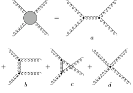
Figure 7: The effective four-gluon vertex and leading order contributions.

Let us define the gluonic contribution, $F^{(g)}_{\eta^{\prime}g^{*}g^{*}}$, to the $\eta^{\prime}g^{*}g^{*}$ vertex as:

$${\cal M}^{(g)}\equiv-i\,F^{(g)}_{\eta^{\prime}g^{*}g^{*}}\,\delta_{ab}\,\varepsilon^{\mu\nu\rho\sigma}\,\varepsilon^{a*}_{\mu}\varepsilon^{b*}_{\nu}q_{1\rho}q_{2\sigma}.$$ (29)

The result of the calculation is:

$$F^{(g)}_{\eta^{\prime}g^{*}g^{*}}(q_{1}^{2},q_{2}^{2},m_{\eta^{\prime}}^{2})=\frac{4\pi\alpha_{s}(Q^{2})}{Q^{2}}\,\frac{C}{2}\int\limits_{0}^{1}dx\,\phi^{(g)}(x,Q)$$

$$\times\left[\frac{xq_{1}^{2}+\bar{x}q_{2}^{2}-(1+x\bar{x})m_{\eta^{\prime}}^{2}}{\bar{x}q_{1}^{2}+xq_{2}^{2}-x\bar{x}m_{\eta^{\prime}}^{2}+i\epsilon}-(x\leftrightarrow\bar{x})\right].$$ (30)

Note that the gluonic wave-function of the $\eta^{\prime}$-meson satisfies the antisymmetry condition $\phi^{(g)}(x,Q)=-\phi^{(g)}(\bar{x},Q)$ Ohrndorf:1981uz ; Shifman:1981dk ; Baier:1981pm . It implies that if the relative sign in the brackets were a “$+$” (as given in Eq. (6) in Ref. Muta ) the gluonic contribution to the $\eta^{\prime}g^{*}g^{*}$ vertex would vanish identically. We disagree with the result stated in Ref. Muta on this point.

When the gluon virtualities are of the same signs, the gluonic contribution to the $\eta^{\prime}g^{*}g^{*}$ vertex can be presented in the form:

$$F^{(g)}_{\eta^{\prime}g^{*}g^{*}}(Q^{2},\omega,\eta)=\frac{4\pi\alpha_{s}(Q^{2})}{Q^{2}}\,2C\omega$$ (31)

$$\times\int\limits_{0}^{1}\frac{(x-\bar{x})\,[1-(1+2x\bar{x})\eta]\,\phi^{(g)}(x,Q)\,dx}{(1-2x\bar{x}\eta)^{2}-\omega^{2}(x-\bar{x})^{2}+i\epsilon},$$

where the total gluon virtuality $q^{2}$, the asymmetry parameter $\omega$, and $\eta$ are the same as the ones entering in Eq. (III) and we have set the scale $Q^{2}=|q^{2}|$. After the integration, and taking into account the gluonic wave-function (7), the result is:

$$F^{(g)}_{\eta^{\prime}g^{*}g^{*}}(Q^{2},\omega,\eta)=\frac{4\pi\alpha_{s}(Q^{2})}{m_{\eta^{\prime}}^{2}}\,\frac{Cq^{2}}{Q^{2}}\,{\rm G}^{(g)}_{2}(\omega,\eta)\qquad$$ (32)

$$\times\left[16B^{(q)}_{2}\left(\frac{\alpha_{s}(Q^{2})}{\alpha_{s}(\mu_{0}^{2})}\right)^{\frac{48}{81}}\!\!\!+5B^{(g)}_{2}\left(\frac{\alpha_{s}(Q^{2})}{\alpha_{s}(\mu_{0}^{2})}\right)^{\frac{101}{81}}\right],$$

where the function ${\rm G}^{(g)}_{2}$ has the following expression:

$${\rm G}^{(g)}_{2}(\omega,\eta) = \omega\Bigg{\{}\frac{5}{3}+\frac{2}{\eta}-\frac{4\omega^{2}}{\eta^{2}}$$

$$+ \frac{1}{2\omega}\left[1-\frac{\omega^{2}}{\eta}\right]\left[1-\frac{4\omega^{2}}{\eta^{2}}\right]\ln\left|\frac{1+\omega}{1-\omega}\right|$$

$$+ \eta\,\left[1-\frac{2}{\eta}-\frac{2+\omega^{2}}{\eta^{2}}+\frac{8\omega^{2}}{\eta^{3}}-\frac{4\omega^{4}}{\eta^{4}}\right]{\rm J}(\omega,\eta)\Bigg{\}}.$$

Note that this function is antisymmetric in its first argument under the change $\omega\to-\omega$: ${\rm G}^{(g)}_{2}(-\omega,\eta)=-{\rm G}^{(g)}_{2}(\omega,\eta)$.

As in the case of the quark-antiquark contribution to the $\eta^{\prime}g^{*}g^{*}$ vertex, the gluonic contribution also contains an imaginary part due to the function ${\rm J}(\omega,\eta)$ as a result of the $i\epsilon$ prescription of the gluon propagator. The imaginary part of the gluonic contribution has a cubic dependence on the total gluon virtuality, ${\rm Im}\,F^{(g)}_{\eta^{\prime}g^{*}g^{*}}\sim(q^{2})^{3}$, in complete analogy with the next-to-leading quark contribution. We use the Brodsky-Lepage prescription discussed in the preceding section and drop the imaginary part in the analysis of the vertex function.

The gluonic contribution to the $\eta^{\prime}g^{*}g^{*}$ vertex has the same $1/Q^{2}$ asymptotics at large $Q^{2}$ ($\eta\to 0$) as the quark contribution (18):

$$F^{(g)}_{\eta^{\prime}g^{*}g^{*}}(Q^{2},\omega,0)=\frac{4\pi\alpha_{s}(Q^{2})}{Q^{2}}\,C\,g_{2}(\omega)$$ (34)

$$\times\left[16B^{(q)}_{2}\left(\frac{\alpha_{s}(Q^{2})}{\alpha_{s}(\mu_{0}^{2})}\right)^{\frac{48}{81}}\!\!\!+5B^{(g)}_{2}\left(\frac{\alpha_{s}(Q^{2})}{\alpha_{s}(\mu_{0}^{2})}\right)^{\frac{101}{81}}\right],$$

$$g_{2}(\omega)=\frac{3f_{0}(\omega)-2}{6\omega},$$ (35)

where the function $f_{0}(\omega)$ is defined by Eq. (19). Note that the gluonic function $g_{2}(\omega)$ is antisymmetric: $g_{2}(-\omega)=-g_{2}(\omega)$, in contrast with the quark functions $f_{i}(-\omega)=f_{i}(\omega)$ ($i=0,2$). The curve corresponding to $g_{2}(\omega)$ is presented in Fig. 4. It takes its maximum and minimum values at the borders of the argument domain: $g_{2}(\pm 1)=\pm 1/6$ and $g_{2}(0)=0$, respectively, because of the antisymmetry condition. Again, as in the next-to-leading order quark contribution to the $\eta^{\prime}g^{*}g^{*}$ vertex, the gluonic contribution has an additional suppression due to the function $g_{2}(\omega)$ for the gluons with comparable virtualities.

For the case when the gluons virtualities have opposite signs ($q_{1}^{2}>0$, $q_{2}^{2}<0$ or $q_{1}^{2}<0$, $q_{2}^{2}>0$), the $\eta^{\prime}g^{*}g^{*}$ vertex can be presented in the form given in Eq. (32) but with a different dependence on the parameters $\omega$ and $\eta$:

$${\rm G}^{(g)}_{2}(\omega,\eta)\to{\rm G}^{(g)}_{2}\left(\frac{1}{\omega},\frac{\eta}{\omega}\right).$$ (36)

The large $Q^{2}$ behavior of the $\eta^{\prime}g^{*}g^{*}$ vertex is the same as in the case of the gluon virtualities of the same signs [Eq. (34)] but involves a different function of the asymmetry parameter:

$$g_{2}(\omega)\to\tilde{g}_{2}(\omega)=\frac{1}{\omega}\,g_{2}\left(\frac{1}{\omega}\right)=-\frac{1}{3}+\omega^{2}-\frac{\omega^{4}}{2}f_{0}(\omega).$$ (37)

The function $\tilde{g}_{2}(\omega)$ is shown graphically in Fig. 5. In contrast to the function $g_{2}(\omega)$, given in Eq. (35), which is antisymmetric in its argument, the function $\tilde{g}_{2}(\omega)$ is symmetric: $\tilde{g}_{2}(-\omega)=\tilde{g}_{2}(\omega)$.

When one of the gluons is on the mass shell, say, the second gluon ($q_{2}^{2}=0$), the leading gluonic contribution to the form factor is:

$$F^{(g)}_{\eta^{\prime}g^{*}g^{*}}(q_{1}^{2},0,m_{\eta^{\prime}}^{2}) = \frac{4\pi\alpha_{s}(|q_{1}^{2}|)}{m_{\eta^{\prime}}^{2}}\,\frac{Cq_{1}^{2}}{|q_{1}^{2}|}\left[16B^{(q)}_{2}\left(\frac{\alpha_{s}(|q_{1}^{2}|)}{\alpha_{s}(\mu_{0}^{2})}\right)^{\frac{48}{81}}\!\!+5B^{(g)}_{2}\left(\frac{\alpha_{s}(|q_{1}^{2}|)}{\alpha_{s}(\mu_{0}^{2})}\right)^{\frac{101}{81}}\right]$$

$$\times \left\{\frac{5}{3}+\frac{2\,q_{1}^{2}}{m_{\eta^{\prime}}^{2}}-\frac{4(q_{1}^{2})^{2}}{m_{\eta^{\prime}}^{4}}-\left[1-\frac{q_{1}^{2}}{m_{\eta^{\prime}}^{2}}\right]\left[1-\frac{4(q_{1}^{2})^{2}}{m_{\eta^{\prime}}^{4}}\right]\ln\left(1-\frac{m_{\eta^{\prime}}^{2}}{q_{1}^{2}}\right)\right\}~{}.$$

In the limit of the large gluon virtuality ($|q_{1}^{2}|\gg m_{\eta^{\prime}}^{2}$) the gluon contribution to the $\eta^{\prime}g^{*}g^{*}$ vertex takes the form:

$$F^{(g)}_{\eta^{\prime}g^{*}g^{*}}(q_{1}^{2},0,0)=\frac{4\pi\alpha_{s}(|q_{1}^{2}|)}{|q_{1}^{2}|}\,\frac{C}{6}\,$$ (39)

$$\times\left[16B^{(q)}_{2}\left(\frac{\alpha_{s}(|q_{1}^{2}|)}{\alpha_{s}(\mu_{0}^{2})}\right)^{\frac{48}{81}}+5B^{(g)}_{2}\left(\frac{\alpha_{s}(|q_{1}^{2}|)}{\alpha_{s}(\mu_{0}^{2})}\right)^{\frac{101}{81}}\right].$$

As noted in the case of the quark contribution, when the gluon virtuality is time-like, $q_{1}^{2}>0$, there is a threshold near $q_{1}^{2}=m_{\eta^{\prime}}^{2}$, but unlike the quark case, the gluonic contribution is regular,

$$F^{(g)}_{\eta^{\prime}g^{*}g^{*}}(m_{\eta^{\prime}}^{2},0,m_{\eta^{\prime}}^{2})=\frac{4\pi\alpha_{s}(m_{\eta^{\prime}}^{2})}{m_{\eta^{\prime}}^{2}}\,\frac{C}{3}\,$$ (40)

$$\times\left[16B^{(q)}_{2}\left(\frac{\alpha_{s}(m_{\eta^{\prime}}^{2})}{\alpha_{s}(\mu_{0}^{2})}\right)^{\frac{48}{81}}+5B^{(g)}_{2}\left(\frac{\alpha_{s}(m_{\eta^{\prime}}^{2})}{\alpha_{s}(\mu_{0}^{2})}\right)^{\frac{101}{81}}\right].$$

We point out that Eq. (IV) is to be used for $|q_{1}^{2}|>m_{\eta^{\prime}}^{2}$ for the space-like gluon virtuality. In the region $0<|q_{1}^{2}|<m_{\eta^{\prime}}^{2}$ the $\eta^{\prime}$-meson mass is the largest scale parameter and in Eq. (IV) the following change should be done: $\alpha_{s}(Q^{2})\to\alpha_{s}(m_{\eta^{\prime}}^{2})$.

V Sudakov-Improved $\eta^{\prime}g^{*}g^{*}$ Vertex

In discussing the $\eta^{\prime}g^{*}g^{*}$ vertex for the situation in which one of the gluons or both are far from the mass shell, the typical mass scale $Q^{2}$ can be defined by the largest virtuality $q_{1}^{2}$ or $q_{2}^{2}$ ($|q_{i}^{2}|\gg m_{\eta^{\prime}}^{2}$). If the transverse momenta ${\bf k}_{\perp i}$ of the partons in the $\eta^{\prime}$-meson are taken into account in the hard scattering approach, the perturbative expansion of the vertex encounters large logarithms of the form $\ln(Q^{2}/{\bf k}_{\perp i}^{2})$, and it becomes mandatory to sum the multiple-gluon emissions. The formalism for the soft and collinear gluon resummation was introduced by Collins and Soper CS and Collins, Soper and Sterman CSS . Such gluon emissions give rise to powers of double logarithms in each order of perturbation theory and their contribution exponentiates into the Sudakov function Sudakov . The Sudakov exponents are known both for quarks from the Drell-Yan (DY) process and the deep inelastic scattering (DIS), and for gluons from the gluon fusion into $2\gamma$, gauge, or Higgs bosons final states. This formalism is also suitable for the description of the hadronic wave-functions and the hadronic form factors, such as the electromagnetic and transition form factors of the pion BS89 ; JKR96 ; JK93 ; Sudakov-gen ; Gousset , and is also of interest here.

In the modified Hard Scattering Approach (mHSA) BS89 , the quark and gluonic invariant amplitudes which define the $\eta^{\prime}g^{*}g^{*}$ vertex can be written as:

$${\cal M}^{(q)} = \frac{1}{\sqrt{2N_{c}}}\int\limits_{0}^{1}dx\int\frac{d{\bf b}}{4\pi}\,\hat{\Psi}^{(q)}(x,Q,{\bf b})\,S^{(q)}(x,Q,b)$$ (41)

$$\times \int\frac{d{\bf k}_{\perp}}{(2\pi)^{2}}\,{\rm e}^{-i({\bf k}_{\perp}{\bf b})}\,{\rm Sp}\{\gamma_{5}(\,\hbox to0.0pt{/\hss}\,\!\!P-m_{\eta^{\prime}})T^{(q)}_{H}\},\qquad$$

$${\cal M}^{(g)} = \frac{-2i}{\sqrt{2N_{c}}}\int\limits_{0}^{1}dx\int\frac{d{\bf b}}{4\pi}\,\hat{\Psi}^{(g)}(x,Q,{\bf b})\,S^{(g)}(x,Q,b)$$ (42)

$$\times \int\frac{d{\bf k}_{\perp}}{(2\pi)^{2}}\,{\rm e}^{-i({\bf k}_{\perp}{\bf b})}\,\varepsilon^{\alpha\beta\mu\nu}\,\frac{q_{1\alpha}q_{2\beta}}{Q^{2}}\,[T^{(g)}_{H}]_{\mu\nu},\qquad$$

where ${\bf b}$ is the separation between the $\eta^{\prime}$ constituents in the transverse configuration space, often called the impact parameter, ${\bf k}_{\perp}$ is the transverse momentum of one of the constituents in the $\eta^{\prime}$-meson rest-frame, and the functions $T^{(q)}_{H}$ and $T^{(g)}_{H}$ are defined in Eqs. (10) and (27), respectively. In this approach we take the $\eta^{\prime}$-meson wave-function in the form similar to the pion wave-function JK93 ; JKR96 :

$$\hat{\Psi}^{(p)}(x,Q,{\bf b})=\frac{2\pi C}{\sqrt{2N_{c}}}\,\phi^{(p)}(x,Q)\,\exp\left[-\frac{x\bar{x}b^{2}}{4a^{2}}\right],$$ (43)

where $p=q$ for quark or antiquark and $p=g$ for gluons, the constant $C$ is defined in Eq. (5), and $\phi^{(q)}$ and $\phi^{(g)}$ have the forms presented in Eqs. (6) and (7), respectively. We assume that the transverse parts of the quark and gluonic components of the $\eta^{\prime}$-meson wave-function are universal and have a simple Gaussian distribution in the separation length $b=|{\bf b}|$, i.e. $\hat{\Psi}^{(p)}(x,Q,{\bf b})=\hat{\Psi}^{(p)}(x,Q,b)$. The parameter $a$ can be determined from the average transverse momentum of the $\eta^{\prime}$-meson. For the numerical analysis we take the transverse size parameter $a^{-1}=0.861$ GeV, obtained for the $\pi$-meson by Kroll et al. JKR96 ; JK93 . The soft-gluon emission from the quark, antiquark and gluons inside the $\eta^{\prime}$-meson can be taken into account by including the QCD Sudakov factors $S^{(p)}(x,Q,b)$ in Eqs. (41) and (42).

We shall perform our analysis by taking into account the next-to-leading logarithmic (NLL) contribution to the Sudakov factors, which are known for both the quark SF-quark and gluonic SF-gluon ; Balazs cases. In applications to form factors of mesons the Sudakov factor is Sudakov-gen :

$$S^{(p)}(x,Q,b)=\exp\left[-s_{p}(xQ,b,C_{1},C_{2})-s_{p}(\bar{x}Q,b,C_{1},C_{2})-\int\limits_{C_{1}^{2}/b^{2}}^{t^{2}}\frac{d\mu^{2}}{\mu^{2}}\gamma_{p}\left(\alpha_{s}(\mu^{2})\right)\right],$$ (44)

where the Sudakov function $s_{p}(Q,b,C_{1},C_{2})$ for an external quark ($p=q$) or gluon ($p=g$) line can be presented in the following general form CSS :

$$s_{p}(Q,b,C_{1},C_{2})=\exp\left\{-\frac{1}{4}\int\limits^{C_{2}^{2}Q^{2}}_{C_{1}^{2}/b^{2}}\frac{dq^{2}}{q^{2}}\left[A_{p}(\alpha_{s}(q^{2}))\ln\frac{C_{2}^{2}Q^{2}}{q^{2}}+B_{p}(\alpha_{s}(q^{2}))\right]\right\}.$$ (45)

The integral term in Eq. (44) arises from the application of the renormalization group to the $\eta^{\prime}$-meson wave-function as well as to the hard scattering amplitude. The upper limit $t^{2}$ is defined by the largest mass scale appearing in the hard scattering amplitude. The functions $\gamma_{p}(\alpha_{s})$ are the anomalous dimensions of the partons inside the $\eta^{\prime}$-meson in the axial gauge BDS :

$$\gamma_{q}(\alpha_{s})=-\frac{3C_{F}\alpha_{s}}{4\pi}+{\cal O}(\alpha_{s}^{2}),\quad\gamma_{g}(\alpha_{s})=-\frac{3\beta_{0}\alpha_{s}}{4\pi}+{\cal O}(\alpha_{s}^{2}).$$ (46)

Notice that as the energy parameter of the Sudakov function one should use the energies $xQ$ and $\bar{x}Q$ of the $\eta^{\prime}$-meson constituents which are, in general, different. The functions $A_{p}(\alpha_{s})$ and $B_{p}(\alpha_{s})$ are perturbatively computable as power series in the strong coupling constant $\alpha_{s}$:

$$A_{p}(\alpha_{s})=\sum_{n=1}^{\infty}\left(\frac{\alpha_{s}}{\pi}\right)^{n}\!\!A_{p}^{(n)},\quad B_{p}(\alpha_{s})=\sum_{n=1}^{\infty}\left(\frac{\alpha_{s}}{\pi}\right)^{n}\!\!B_{p}^{(n)},$$ (47)

where $A_{p}^{(n)}$ and $B_{p}^{(n)}$ are the expansion coefficients, specified below for $n=1$ and $n=2$. We recall that the coefficients $A_{p}^{(1)}$ are universal and lead to the resummation of the leading logarithmic (LL) contributions. The coefficients $A_{p}^{(2)}$ and $B_{p}^{(1)}$ give the NLL terms. These coefficients are also process-independent but they depend on the renormalization and factorization schemes through the parameters $C_{1}$ and $C_{2}$. The next expansion coefficients are process-dependent, as demonstrated recently for $B_{p}^{(2)}$ CdFG . However, to the NLL accuracy, we do not require them. The coefficients of the LL and NLL terms of the Sudakov exponent for quarks CSS ; SF-quark ; DS and gluons SF-gluon ; Balazs are:

$$A_{q}^{(1)} = C_{F},\qquad A_{g}^{(1)}=C_{A},$$

$$A_{q}^{(2)} = \frac{1}{2}C_{F}\left[K+\beta_{0}\ln\frac{C_{1}}{b_{0}}\right],$$

$$A_{g}^{(2)} = \frac{1}{2}C_{A}\left[K+\beta_{0}\ln\frac{C_{1}}{b_{0}}\right],$$ (48)

$$B_{q}^{(1)} = -\frac{1}{2}C_{F}\left[1+2\ln\frac{C_{2}b_{0}}{C_{1}}\right],$$

$$B_{g}^{(1)} = -\frac{\beta_{0}}{2}-6\ln\frac{C_{2}b_{0}}{C_{1}},$$

where $C_{F}=(N_{c}^{2}-1)/(2N_{c})$, $C_{A}=N_{c}$ ($N_{c}=3$ in QCD), $b_{0}=2\exp(-\gamma_{E})$ where $\gamma_{E}$ is the Euler constant, $n_{f}$ is the number of active quarks (with masses $m_{q}<C_{2}Q$), the coefficient $K$ SF-quark is:

$$K=C_{A}\left[\frac{67}{18}-\frac{\pi^{2}}{6}\right]-\frac{5}{9}\,n_{f},$$

and $\beta_{0}$ has been specified earlier in Eq. (8). Note that the coefficient $B_{q}^{(1)}$ given above in Eq. (48) is taken from Ref. Stefanis99 and it differs from the corresponding coefficient given in Ref. SF-gluon .

The knowledge of the LL and NLL perturbative coefficients $A_{p}^{(1)}$, $A_{p}^{(2)}$, and $B_{p}^{(1)}$ as well as the strong coupling $\alpha_{s}(q^{2})$ at the two-loop level (8) allows to get the explicit expression for the LL and NLL terms of the Sudakov functions in the form:

$$s_{p}(Q,b,C_{1},C_{2})=\frac{A_{p}^{(1)}}{\beta_{0}}\,L_{Q}\left[\ln\lambda+\frac{1}{\lambda}-1\right]$$ (49)

$$-\frac{4A_{p}^{(2)}}{\beta_{0}^{2}}\left[\ln\lambda-\lambda+1\right]+\frac{B_{p}^{(1)}}{\beta_{0}}\,\ln\lambda+\frac{2\beta_{1}A_{p}^{(1)}}{\beta_{0}^{3}}$$

$$\times\left[\lambda\,\ln\lambda+(1-\lambda)\,(1+\ln L_{Q})+\ln L_{Q}\,\ln\lambda-\frac{1}{2}\ln^{2}\lambda\right],$$

where $\lambda=L_{Q}/L_{b}$, $L_{Q}=\ln(C_{2}^{2}Q^{2}/\Lambda^{2})$, and $L_{b}=\ln(C_{1}^{2}/b^{2}\Lambda^{2})$.

Let us discuss the range of the impact parameter $b$. In general, it is defined as a positive variable but in the region $b\geq 1/\Lambda$ the Sudakov exponent diverges due to the Landau pole in the QCD coupling $\alpha_{s}(\mu^{2})$ at $\mu=\Lambda$. In this case the perturbative calculation is no longer valid and a prescription for parametrizing the non-perturbative physics in the low transverse momentum (or large $b$) region is necessary. We shall restrict ourselves to the region $b<1/\Lambda$. There also exists a lower bound on the Sudakov function, arising from the consideration that the transverse momentum of the emitted gluons is not allowed to be large, i.e., we have to restrict to the region $|{\bf k}_{\perp}|\ll C_{2}Q$, where $C_{2}Q$ is the hard scale. Thus, the region of applicability of the Sudakov formalism is limited to the region: $1/C_{2}Q\ll b\ll 1/\Lambda$.

In the following it is necessary to fix the arbitrary parameters $C_{1}$ and $C_{2}$. The constant $C_{1}$ determines the onset of the non-perturbative physics. The renormalization constant $C_{2}$ specifies the scale of the hard scattering process. Following Ref. Sudakov-gen , we make the choice $C_{1}=1$ and $C_{2}=1/\sqrt{2}$ in our analysis.

Using the definitions of the $\bar{q}q$ and gluonic parts of the $\eta^{\prime}$-meson vertex (12) and (29), respectively, the results for the corresponding vertices, including the dependence on the transverse momenta, are:

$$F^{(q)}_{\eta^{\prime}g^{*}g^{*}}(q_{1}^{2},q_{2}^{2},m_{\eta^{\prime}}^{2})=4\pi\alpha_{s}(Q^{2})\,\frac{2}{\sqrt{2N_{c}}}$$ (50)

$$\times\int\limits_{0}^{1}\!dx\!\!\int\!\frac{d{\bf b}}{4\pi}\hat{\Psi}^{(q)}(x,Q,{\bf b})\,S^{(q)}(x,Q,b)\int\!\frac{d{\bf k}_{\perp}}{(2\pi)^{2}}\,{\rm e}^{-i({\bf k}_{\perp}{\bf b})}$$

$$\times\left[\frac{1}{xq_{1}^{2}+\bar{x}q_{2}^{2}-x\bar{x}m_{\eta^{\prime}}^{2}-{\bf k}_{\perp}^{2}+i\epsilon}+(x\leftrightarrow\bar{x})\right],$$

$$F^{(g)}_{\eta^{\prime}g^{*}g^{*}}(q_{1}^{2},q_{2}^{2},m_{\eta^{\prime}}^{2})=\frac{4\pi\alpha_{s}(Q^{2})}{Q^{2}}\,\sqrt{2N_{c}}$$ (51)

$$\times\int\limits_{0}^{1}\!dx\!\!\int\!\frac{d{\bf b}}{4\pi}\hat{\Psi}^{(g)}(x,Q,{\bf b})\,S^{(g)}(x,Q,b)\int\!\frac{d{\bf k}_{\perp}}{(2\pi)^{2}}\,{\rm e}^{-i({\bf k}_{\perp}{\bf b})}$$

$$\times\left[\frac{m_{\eta^{\prime}}^{2}+(x-\bar{x})(q_{1}^{2}-q_{2}^{2})}{xq_{1}^{2}+\bar{x}q_{2}^{2}-x\bar{x}m_{\eta^{\prime}}^{2}-{\bf k}_{\perp}^{2}+i\epsilon}-(x\leftrightarrow\bar{x})\right].$$

For the space-like gluon virtualities [$q_{1}^{2}<0$, $q_{2}^{2}<0$, and $Q^{2}=-(q_{1}^{2}+q_{2}^{2})$] the integration over the transverse momentum ${\bf k}_{\perp}$ can be done resulting in the modified Bessel function of order zero, $K_{0}(z)$. Taking this into account and substituting the $\eta^{\prime}$-meson wave-function (43), the quark and gluonic contributions reduce to the two-dimensional integrals of the form:

$$F^{(q)}_{\eta^{\prime}g^{*}g^{*}}(Q,\omega,\eta) = -4\pi\alpha_{s}(Q^{2})\,\frac{C}{N_{c}}\int\limits_{0}^{1}dx\,\phi^{(q)}(x,Q)\int\limits_{0}^{\infty}db\,b\,{\rm e}^{-x\bar{x}b^{2}/4a^{2}}\,S^{(q)}(x,Q,b)\,K^{(+)}_{0}(x,bQ)$$

$$= -4\pi\alpha_{s}(Q^{2})\,\frac{C}{N_{c}\Lambda^{2}}\int\limits_{0}^{1}dx\,\phi^{(q)}(x,Q)\int\limits_{0}^{1}db_{\Lambda}\,b_{\Lambda}\,\exp\left[-\frac{x\bar{x}}{4a^{2}\Lambda^{2}}\,b_{\Lambda}^{2}\right]\,S^{(q)}(x,Q,b)\,K_{0}^{(+)}(x,b_{\Lambda}Q_{\Lambda}),$$

$$F^{(g)}_{\eta^{\prime}g^{*}g^{*}}(Q,\omega,\eta) = -4\pi\alpha_{s}(Q^{2})\,C\int\limits_{0}^{1}dx\,\phi^{(g)}(x,Q)\int\limits_{0}^{\infty}db\,b\,{\rm e}^{-x\bar{x}b^{2}/4a^{2}}\,S^{(g)}(x,Q,b)$$

$$\times \left[|\eta|\,K^{(-)}_{0}(x,bQ)-(x-\bar{x})\,\omega\,K^{(+)}_{0}(x,bQ)\right]$$

$$= -4\pi\alpha_{s}(Q^{2})\,\frac{C}{\Lambda^{2}}\int\limits_{0}^{1}dx\,\phi^{(g)}(x,Q)\int\limits_{0}^{1}db_{\Lambda}\,b_{\Lambda}\,\exp\left[-\frac{x\bar{x}}{4a^{2}\Lambda^{2}}\,b_{\Lambda}^{2}\right]\,$$

$$\times S^{(g)}(x,Q,b)\,\left[|\eta|K_{0}^{(-)}(x,b_{\Lambda}Q_{\Lambda})-(x-\bar{x})\omega K_{0}^{(+)}(x,b_{\Lambda}Q_{\Lambda})\right],$$

where

$$K^{(\pm)}_{0}(x,bQ)=K^{(\pm)}_{0}(x,b_{\Lambda}Q_{\Lambda})=\frac{1}{2}\left[K_{0}\left(b_{\Lambda}Q_{\Lambda}\lambda_{+}(x,\omega,\eta)\right)\pm K_{0}\left(b_{\Lambda}Q_{\Lambda}\lambda_{+}(\bar{x},\omega,\eta)\right)\right],$$

with the dimensionless parameters defined as $b_{\Lambda}=b\Lambda$, $Q_{\Lambda}=Q/\Lambda$, $|\eta|=m_{\eta^{\prime}}^{2}/Q^{2}$; the function $\lambda_{\pm}^{2}(x,\omega,\eta)=[1+\omega(x-\bar{x})\pm 2x\bar{x}|\eta|]/2$, and the quark and gluonic components of the $\eta^{\prime}$-meson wave-function are taken in the form of Eq. (43). The restriction $b\leq 1/\Lambda$ due to the Sudakov formalism is also taken into account in the final result for the space-like gluons presented in Eqs. (V) and (V).

The arguments of the Bessel functions $K_{0}(bQ\lambda_{+}(x,\omega,\eta))$ and $K_{0}(bQ\lambda_{+}(\bar{x},\omega,\eta))$ in the $\eta^{\prime}$-meson vertex define the largest scale parameter $t$ in the Sudakov factor (44):

$$t=\max\left\{Q\lambda_{+}(x,\omega,\eta),Q\lambda_{+}(\bar{x},\omega,\eta),1/b\right\}.$$ (54)

The dependence of the Sudakov factors $S^{(q)}(x,Q,b)$ and $S^{(g)}(x,Q,b)$ on the impact parameter $b$ at $x=1/2$ and $Q=10\Lambda$, $20\Lambda$ and $50\Lambda$ is presented in Fig. 8.

Figure 8: The Sudakov function plotted in terms of the dimensionless impact parameter $b_{\Lambda}$ for quarks (upper figure) and gluons (lower figure) with $x=1/2$ and $Q=10\Lambda$, $20\Lambda$, and $50\Lambda$.

It is seen that the Sudakov factors give a cut-off in addition to the restriction $b\leq 1/\Lambda$ of the cut-off of the integration interval over $b$. With increasing the typical mass scale $Q$ this effect is stronger in the quark contribution.

In Fig. 9 we show the distribution of the quark and gluonic parts of the vertex in the impact parameter space integrating here with a variable cut off, $b_{cut}$. The curves, showing the dependence of $q_{1}^{2}\,F^{(p)}_{\eta^{\prime}g^{*}g}(q_{1}^{2},0,m_{\eta^{\prime}}^{2})$ on $b_{cut}$, start from zero for $b_{cut}=0$ and reach their full height for $b_{cut}=1$ beyond which we consider any remaining contributions as non-perturbative.

Figure 9: The quark-antiquark (upper figure) and gluonic (lower figure) contributions to the $\eta^{\prime}g^{*}g$ vertex function $q_{1}^{2}F^{(p)}_{\eta^{\prime}g^{*}g}(q_{1}^{2},0,m_{\eta^{\prime}}^{2})$ versus the cut off in the impact parameter space, $b_{cut}$, for the space-like gluon virtuality $q_{1}^{2}=-Q^{2}$ with $Q=10\Lambda$, $20\Lambda$, and $50\Lambda$.

The faster rise of the $\eta^{\prime}g^{*}g^{*}$ vertex is observed for the quark contribution as $Q$ increases while the gluonic one is mildly sensitive to the typical mass scale. At the largest value shown, $Q=50\Lambda$, the quark curve is quite flat for $b_{cut}\geq 0.2$ which indicates a small contribution from this region. As for the smaller values, for example, $Q=10\Lambda$, the vertex gets a rather large contribution from large distances in the impact parameter space. The gluonic part of the vertex receives the main contribution from the short distances $b\leq 0.3$. In contrast to the quark contribution, the gluonic contribution is negative and decreases the summed vertex function by approximately 20%.

To obtain the $\eta^{\prime}$-meson vertex function for the time-like gluon virtualities one has to replace $Q^{2}\to-Q^{2}$ and $|\eta|\to-\eta$ in Eqs. (V) and (V). The vertex function is an analytic function of the scale parameter $Q^{2}$ and it can be analytically continued from the space-like $Q^{2}$ region to the time-like one. As mentioned earlier, the $\eta^{\prime}g^{*}g^{*}$ vertex results from convoluting the $\eta^{\prime}$-meson wave-function and the hard scattering amplitude kernel. As we do not take the QCD corrections to the hard scattering amplitude into account, the strong coupling, $\alpha_{s}(q^{2})$, has the same dependence on the scale parameter in both the space-like and time-like regions ($\alpha_{s}(-q^{2})=\alpha_{s}(q^{2})[1+{\cal O}(\alpha_{s})]$). The other component of the $\eta^{\prime}$-meson wave-function sensitive to the transition from the space-like region to the time-like one is the Sudakov factor (44). The analytic continuation of the Sudakov factor was analyzed in Refs. MS90 ; Gousset with the result that the time-like and space-like form factors have the same scale dependence in the asymptotic regime. We use the space-like expression for the Sudakov factor to study the $\eta^{\prime}g^{*}g^{*}$ vertex for the time-like gluon virtualities. The hard scattering amplitude kernel gives the additional transfer momentum dependence due to the quark and gluon propagators. We recall that, in general, the propagator is defined in the complex momentum plane and, hence, it can have both real and imaginary parts in the time-like region of the momentum due to $i\epsilon$ term in the denominator. Here, we perform the analysis of the propagators in the transverse momentum space keeping their transverse momenta dependence. In mHSA it is more convenient to operate with the Fourier transform of the propagators in the impact parameter space but this analysis can be easily reformulated in terms of the impact parameter ${\bf b}$, which is the conjugate variable to ${\bf k}_{\perp}$.

The ${\bf k}_{\perp}$ integration plane can be divided in several regions as shown in Fig. 10. The interval $0<|{\bf k}_{\perp}|<\Lambda$ is the non-perturbative region. We note that the Brodsky-Lepage approach, in which the dependence on the transverse momentum is neglected, corresponds to the point ${\bf k}_{\perp}=0$ in Fig. 10. It is seen that this transverse momentum value lies in the deeply non-perturbative region and too far from the contributing region of the transverse momentum integration. It means that in the Brodsky-Lepage approach the imaginary part of the $\eta^{\prime}g^{*}g^{*}$ vertex can not be calculated correctly and the natural prescription is to drop it altogether. Another consequence of the approximate forms of the propagators in the Brodsky-Lepage picture is the appearance of the singularity in the $\eta^{\prime}g^{*}g^{*}$ vertex in the region close to the $\eta^{\prime}$-meson mass. The interval $|{\bf k}_{\perp}|>\Lambda$ can be effectively divided into two regions: the soft-gluon region (SGR) where the Sudakov factor is taken into account and the hard-gluon region (HGR) where the Sudakov effect is absent. In Fig. 10 we also point out the value of $\sqrt{x\bar{x}}a^{-1}$ to show the importance of the transverse momentum distribution of the $\eta^{\prime}$-meson wave-function. In the region $|{\bf k}_{\perp}|>\sqrt{x\bar{x}}a^{-1}$ the contribution to the vertex is effectively suppressed by the assumed Gaussian behavior of the transverse momentum distribution (43).

Figure 10: Different regions in the integration plane in the variable ${\bf k}_{\perp}$. The abbreviations used correspond to non-perturbative (NPR), soft-gluon (SGR), and hard-gluon (HGR) regions. The point $|{\bf k}_{\perp}|=0$ corresponds to the Brodsky-Lepage approach.

To calculate the integrals (50) and (51) over the transverse momentum ${\bf k}_{\perp}$ in the time-like region of the gluon virtualities it is useful to do the analytic continuation of $|{\bf k}_{\perp}|$ in the complex plane. The new feature with respect to the space-like case is that the contour of the transverse momentum integration goes now near the pole located at ${\bf k}_{\perp}^{2}=Q^{2}\,\lambda_{-}^{2}+i\epsilon$. This pole, except in the end point regions [$x\to 0$ for the second gluon on the mass shell, or $x\to 1$ for the first one due to the function $\lambda_{-}(x,\omega,\eta)$], is far from the bounds of integration of the variable $|{\bf k}_{\perp}|$. Therefore, this integral can be evaluated by deforming the contour of the integration in the complex plane of this variable.

The pole encountered in our computations when an internal quark or gluon goes on the mass shell do not correspond to an observable state. They appear in the effective $\eta^{\prime}g^{*}g^{*}$ vertex which is not an observable by itself. Provided this vertex is included in the complete amplitude of some real process such as $B\to\eta^{\prime}K$ and $B\to\eta^{\prime}X_{s}$, this amplitude will have an additional complex phase factor as a reminder of this singularity. Notice that the complete physical amplitude of the process including the effective $\eta^{\prime}g^{*}g^{*}$ vertex in a purely hadronic computations has also the poles reflecting the existence of the intermediate physical (mass-shell) states which are hadronic ones. Therefore, it is natural to expect the appearance of the additional phase factor here also.

According to the arguments given above, the $\eta^{\prime}g^{*}g^{*}$ vertex for the time-like gluon virtualities can be obtained from Eqs. (V) and (V) by changing $|\eta|\to-\eta$ and $K_{0}(bQ\lambda_{+}(x,\omega,\eta))\to K_{0}(ibQ\lambda_{-}(x,\omega,\eta))$. If one uses the relation $K_{0}(iz)=-i\pi\,H_{0}^{(2)}(z)/2$ where $H_{0}^{(2)}(z)=J_{0}(z)-iY_{0}(z)$, (here, $H_{0}^{(2)}(z)$, $J_{0}(z)$ and $Y_{0}(z)$ are the second Hankel function, Bessel function of the first kind, and Neumann function, respectively Bateman ), it is seen that in contrast to the case of the space-like gluon virtualities the vertex gets an imaginary part. After these changes the quark and gluonic contributions to the $\eta^{\prime}g^{*}g^{*}$ vertex function are:

$$F^{(q)}_{\eta^{\prime}g^{*}g^{*}}(Q,\omega,\eta) = 4\pi\alpha_{s}(Q^{2})\,\frac{i\pi C}{2N_{c}\Lambda^{2}}\int\limits_{0}^{1}dx\,\phi^{(q)}(x,Q)\int\limits_{0}^{1}db_{\Lambda}\,b_{\Lambda}\,\exp\left[-\frac{x\bar{x}}{4a^{2}\Lambda^{2}}\,b_{\Lambda}^{2}\right]\,S^{(q)}(x,Q,b)\,H_{0}^{(+)}(x,b_{\Lambda}Q_{\Lambda}),\qquad$$ (55)

$$F^{(g)}_{\eta^{\prime}g^{*}g^{*}}(Q,\omega,\eta) = 4\pi\alpha_{s}(Q^{2})\,\frac{i\pi C}{2\Lambda^{2}}\int\limits_{0}^{1}dx\,\phi^{(g)}(x,Q)\int\limits_{0}^{1}db_{\Lambda}\,b_{\Lambda}\,\exp\left[-\frac{x\bar{x}}{4a^{2}\Lambda^{2}}\,b_{\Lambda}^{2}\right]\qquad$$

$$\times S^{(g)}(x,Q,b)\,\left[\eta H_{0}^{(-)}(x,b_{\Lambda}Q_{\Lambda})+(x-\bar{x})\omega H_{0}^{(+)}(x,b_{\Lambda}Q_{\Lambda})\right],$$

where

$$H_{0}^{(\pm)}(x,bQ)=H_{0}^{(\pm)}(x,b_{\Lambda}Q_{\Lambda})=\frac{1}{2}\left[H^{(2)}_{0}\left(b_{\Lambda}Q_{\Lambda}\lambda_{-}(x,\omega,\eta)\right)\pm H^{(2)}_{0}\left(b_{\Lambda}Q_{\Lambda}\lambda_{-}(\bar{x},\omega,\eta)\right)\right].$$

The real and imaginary parts of the $\eta^{\prime}g^{*}g^{*}$ vertex in the form $q_{1}^{2}\,F^{(p)}_{\eta^{\prime}g^{*}g}$ are shown as functions of the impact parameter cut off, $b_{cut}$, in Fig. 11.

Figure 11: The real (solid curves in the upper figure) and imaginary parts (dashed curves in the upper figure) and the absolute value of the vertex function $q_{1}^{2}F_{\eta^{\prime}g^{*}g}(q_{1}^{2},0,m_{\eta^{\prime}}^{2})$ (lower figure), plotted as functions of the cut off, $b_{cut}$, in the impact parameter space for the time-like gluon virtuality, $q_{1}^{2}=Q^{2}$, with $Q=10\Lambda$, $20\Lambda$, and $50\Lambda$.

As in the case of the space-like virtualities, a fast rise is observed with $Q$ in the region of small values of the impact parameter cut-off. The oscillatory behavior of the cylindric functions results in an oscillatory form of the vertex function for small and moderate values of the impact parameter. The contribution to the vertex from the large distances, $b\geq 0.8$, is small. It is also seen that as the scale parameter $Q$ increases, the relative contribution of the imaginary part in the absolute value of the vertex is strongly suppressed, and the vertex is mainly defined by the real contribution in the large $Q^{2}$ asymptotics.

The asymptotics of the quark part of the vertex $F_{\eta^{\prime}g^{*}g^{*}}^{(q)}$ in the limit of large $Q^{2}$ is:

$$F_{\eta^{\prime}g^{*}g^{*}}^{(q)} \simeq 4\pi\alpha(Q^{2})\,\frac{3C}{N_{c}Q^{2}}\,\left\{f_{0}(\omega)+\frac{2i\pi}{\omega}\,y_{+}y_{-}\right.$$

$$\times \left.\vphantom{\frac{2i\pi}{\omega}\,y_{+}y_{-}\,}(1-y_{+}y_{-})\left[H_{0}^{(2)}(Q_{\Lambda}y_{+})-H_{0}^{(2)}(Q_{\Lambda}y_{-})\right]\right\},$$

where $y_{\pm}=\sqrt{(1\pm\omega)/2}$, and the function $f_{0}(\omega)$ is defined in Eq. (19). In this expression the large argument asymptotics of the Hankel function should be used: $H_{0}^{(2)}(z)\simeq\sqrt{2/\pi z}\,\exp(-i[z-\pi/4])$ Bateman . The same correction of order $1/Q^{5/2}$ to the gluonic part of the vertex function $F_{\eta^{\prime}g^{*}g^{*}}^{(g)}$ is equal to zero and one can use the asymptotic behavior defined by Eq. (34).

VI Numerical Analysis and Comparison with Existing Results

In this section we give a numerical analysis of the $\eta^{\prime}g^{*}g^{*}$ vertex in the time-like and space-like regions, derived in the preceding sections. To that end we specify the input parameters. The dimensional factor $C$ [see Eq. (5)] contains the decay constants $f_{q}$ and $f_{s}$ and the mixing angle $\phi$ which can be constrained from the existing experimental data. We shall adopt here the Feldmann-Kroll-Stech $\eta-\eta^{\prime}$ mixing scheme FKS98 , which is phenomenologically consistent and satisfies the constraints from chiral perturbation theory Leutwyler , yielding FKS98 : $f_{q}=(1.07\pm 0.02)\,f_{\pi}$, $f_{s}=(1.34\pm 0.06)\,f_{\pi}$, and $\phi=39.3^{\circ}\pm 1.0^{\circ}$, where $f_{\pi}\simeq 131$ MeV is the pion decay constant. Using the central values of the parameters, one gets $C\simeq 2f_{\pi}\simeq 260$ MeV.

The quark and gluonic wave-functions (63) and (64) contain both free ($B^{(q)}_{n}$, $B^{(g)}_{n}$) and constrained ($\rho^{(q)}_{n}$, $\rho^{(g)}_{n}$) parameters. The constrained parameters depend on the anomalous dimensions and are given in Appendix A, while the free parameters can be fitted from the experimental data, for example, from the $\eta^{\prime}\gamma^{*}\gamma$ transition form factor. We take the following restrictions on the first correction to the leading order wave-function (63): $|B^{(q)}_{2}|<0.1$ and $|\rho^{(g)}_{2}\,B^{(g)}_{2}|<0.1$ in order to keep $\phi^{(q)}(x,Q)$ close to its asymptotic value: $\phi_{\rm as}(x)=6x\bar{x}$, in agreement with the experimental data on the $\eta^{\prime}\gamma^{*}\gamma$ transition form factor eta'-gamma . Taking into account $\rho^{(g)}_{2}\simeq-1/90$ from Eq. (76) we get $|B^{(g)}_{2}|<9.0$. Below, we shall present the $\eta^{\prime}g^{*}g^{*}$ vertex function for the maximum allowed values of the non-perturbative parameters, i.e., $|B^{(q)}_{2}|=0.1$ and $|B^{(g)}_{2}|=9.0$. We have also studied numerically the resulting vertex function for considerably smaller values of these parameters. In that context we note that as the NLO quark contribution to the overall $\eta^{\prime}g^{*}g^{*}$ vertex function is small, there is not much sensitivity to the variation of the parameter $B^{(q)}_{2}$. Hence, we fix this parameter to its maximum allowed value $|B^{(q)}_{2}|=0.1$. However, there is considerable sensitivity to the variation of the parameter $B^{(g)}_{2}$. To show this we shall take $|B^{(g)}_{2}|=3.0$. The resulting theoretical dispersion between the two cases ($|B^{(g)}_{2}|=9.0$ vs. $|B^{(g)}_{2}|=3.0$) can be taken as representative of the theoretical uncertainties due to the undetermined non-perturbative parameters.

First, we consider the case when one of the gluons is on the mass shell, which we take for the sake of definiteness to be the second one ($q_{2}^{2}=0$). In Fig. 12 we show the leading (long-dashed curve) and next-to-leading (middle-dashed curve) quark contributions as well as the gluonic one (short-dashed curve) for the time-like gluon virtuality ($q_{1}^{2}>m_{\eta^{\prime}}^{2}$) corresponding to the maximal values of the free parameters: $B^{(q)}_{2}=0.1$ and $B^{(g)}_{2}=9.0$ (upper plot), and for $B^{(q)}_{2}=0.1$ and $B^{(g)}_{2}=3.0$ (lower plot). The solid curve in each of these figures is the total contribution to $F_{\eta^{\prime}g^{*}g^{*}}(q_{1}^{2},0,m_{\eta^{\prime}}^{2})$ in next-to-leading order.

Figure 12: The $\eta^{\prime}g^{*}g$ vertex $F_{\eta^{\prime}g^{*}g^{*}}(q_{1}^{2},0,m_{\eta^{\prime}}^{2})$ as a function of $q_{1}^{2}$ with $B^{(q)}_{2}=0.1$ and two values of $B^{(g)}_{2}$: $B^{(g)}_{2}=9.0$ (the upper plot) and $B^{(g)}_{2}=3.0$ (the lower plot) in the Brodsky-Lepage approach. The dashed curves are the leading (LQ), next-to-leading quark-antiquark (NLQ), and gluonic (NLG) components, and the solid curve is the sum.

One can see from this figure that with the given parameters, the next-to-leading quark contribution is subdominant in the entire region of $Q^{2}$ shown, except in the neighborhood of the threshold $Q^{2}=m_{\eta^{\prime}}^{2}$, where both the leading and non-leading quark contributions have logarithmic divergences. Notice that in this region our results are not valid and we can trust only the region $Q^{2}\gg m_{\eta^{\prime}}^{2}$. The gluonic contribution (called NLG) for the maximum values of the free parameters is comparable to the leading quark contribution (called LQ), as shown in the upper plot in Fig. 12, increasing the $\eta^{\prime}g^{*}g$ vertex by almost a factor 2 as compared to the case when only the quark content of the $\eta^{\prime}$-meson is assumed. This may be considered as the maximum gluonic content of the $\eta^{\prime}$-meson allowed by current data. Even in the more realistic case with $B^{(q)}_{2}=0.1$ and $B^{(g)}_{2}=3.0$, we see from the lower plot in Fig. 12 that the gluonic contribution is not small, and also in this case it enhances the value of the total $\eta^{\prime}g^{*}g$ vertex function (the solid curve in Fig. 12) at the level of few tens percent.

Let us compare the $\eta^{\prime}g^{*}g$ vertex calculated here with the two set of values $B^{(q)}_{2}=0.1$ and $B^{(g)}_{2}=9.0$ (the upper solid curve in Fig. 13) and $B^{(q)}_{2}=0.1$ and $B^{(g)}_{2}=3.0$ (the lower solid curve in Fig. 13) with the ones given in the literature.

Figure 13: The $\eta^{\prime}g^{*}g$ vertex for the time-like gluon virtuality with $B^{(q)}_{2}=0.1$ and two values of $B^{(g)}_{2}$: $B^{(g)}_{2}=9.0$ (upper solid curve) and $B^{(g)}_{2}=3.0$ (lower solid curve) calculated in the Brodsky-Lepage approach in this paper. The long- and short-dashed curves correspond to the functions $F^{(KP)}_{\eta^{\prime}g^{*}g}(q_{1}^{2},0,m_{\eta^{\prime}}^{2})=1.8~{}{\rm GeV}^{-1}/(q_{1}^{2}/m_{\eta^{\prime}}^{2}-1)$ TFF-1 and $F^{(HT)}_{\eta^{\prime}g^{*}g}(Q^{2})=\sqrt{3}\alpha_{s}(Q^{2})/(\pi f_{\pi})$ TFF-2 , respectively. A constant form of the vertex function $F^{(AS)}_{\eta^{\prime}g^{*}g}=1.8~{}{\rm GeV}^{-1}$ suggested in Ref. TFF-3 is also shown as a dashed line.

In Ref. TFF-1 , Kagan and Petrov have parametrized the $\eta^{\prime}g^{*}g$ vertex in the form: $F_{\eta^{\prime}g^{*}g}(q_{1}^{2},0,m_{\eta^{\prime}}^{2})=H(0,0,m_{\eta^{\prime}}^{2})/(q_{1}^{2}/m_{\eta^{\prime}}^{2}-1)$, where $H(0,0,m_{\eta^{\prime}}^{2})\simeq 1.8~{}{\rm GeV}^{-1}$ is a phenomenological parameter extracted from the experimental data. Its behavior is described by the long-dashed curve in Fig. 13, labeled as $F_{\eta^{\prime}g^{*}g}^{(KP)}$ . In Ref. TFF-2 , Hou and Tseng have parametrized the $\eta^{\prime}g^{*}g$ vertex as: $F_{\eta^{\prime}g^{*}g}(q_{1}^{2})=\sqrt{3}\alpha_{s}(q_{1}^{2})/(\pi f_{\pi})$, which is drawn as the short-dashed curve in Fig. 13, labeled as $F_{\eta^{\prime}g^{*}g}^{(HT)}$. Finally, we also show the constant vertex function $F_{\eta^{\prime}g^{*}g}(q_{1}^{2})=F_{\eta^{\prime}g^{*}g}^{(AS)}=1.8~{}{\rm GeV}^{-1}$, assumed by Atwood and Soni in Ref. TFF-3 . It is seen that our result (the upper solid curve) compares well with the form used in Ref. TFF-1 for a wide range of $q_{1}^{2}$, but is significantly different (smaller) than the one assumed in Ref. TFF-2 and is in complete disagreement with the one assumed in Ref. TFF-3 . Our analysis shows that in the case of the lower possible values of the free parameters: $B^{(q)}_{2}=-0.1$ and $B^{(g)}_{2}=-9.0$, the vertex function $F_{\eta^{\prime}g^{*}g^{*}}(q_{1}^{2},0,m_{\eta^{\prime}}^{2})$ decreases and a substantial disagreement with the vertex suggested in Ref. TFF-1 would result. However, as discussed below, data on the electromagnetic transition form factor of the $\eta^{\prime}$-meson disfavors this choice of the parameters.

We show the results of our calculations for the function $q_{1}^{2}\,F_{\eta^{\prime}g^{*}g}(q_{1}^{2})$ in the space-like region of the gluon virtuality ($q_{1}^{2}=-Q^{2}<0$) in Fig. 14.

Figure 14: The $\eta^{\prime}g^{*}g$ vertex function $q_{1}^{2}\,F_{\eta^{\prime}g^{*}g}(q_{1}^{2})$ for the space-like gluon virtuality with $B^{(q)}_{2}=-0.1$, $B^{(g)}_{2}=-9.0$ and $B^{(q)}_{2}=0.1$, $B^{(g)}_{2}=9.0$ (the upper and lower solid curves) and $B^{(q)}_{2}=-0.1$, $B^{(g)}_{2}=-3.0$ and $B^{(q)}_{2}=0.1$, $B^{(g)}_{2}=3.0$ (the upper and lower dotted curves) in the Brodsky-Lepage approach. The dashed curve is the leading order contribution to the function obtained by setting $B^{(q)}_{2}=B^{(g)}_{2}=0$.

The dashed curve in the middle is the leading contribution to the $\eta^{\prime}g^{*}g$ vertex, obtained by setting the non-asymptotic parameters $B_{2}^{(q)}$ and $B_{2}^{(g)}$ equal to zero. The upper and lower solid curves are the vertex functions $F_{\eta^{\prime}g^{*}g}(q_{1}^{2},0,m_{\eta^{\prime}}^{2})$ taking into account the next-to-leading correction with $B^{(q)}_{2}=-0.1$, $B^{(g)}_{2}=-9.0$ (upper curve) and $B^{(q)}_{2}=0.1$, $B^{(g)}_{2}=9.0$ (lower curve). The dotted curves correspond to the choice $B^{(q)}_{2}=-0.1$, $B^{(g)}_{2}=-3.0$ (upper curve) and $B^{(q)}_{2}=0.1$, $B^{(g)}_{2}=3.0$ (lower curve). We note that the correction is mainly determined by the value of the parameter $B^{(g)}_{2}$. It is seen that at small values of the gluon virtuality ($Q^{2}<5$ GeV²) the complete correction becomes approximately equal to or even larger than the leading order contribution. This implies that in the region $Q^{2}<$ few GeV² our approximation is not valid and the contributions of the next higher order corrections become important. The behavior of $F_{\eta^{\prime}g^{*}g}(Q^{2},0,m_{\eta^{\prime}}^{2})$ for large $Q^{2}$ is in qualitative agreement with the corresponding electromagnetic transition form factor, $F_{\eta^{\prime}\gamma^{*}\gamma}(Q^{2},0,m_{\eta^{\prime}}^{2})$, measured in $\gamma\gamma^{*}$-collisions, more recently by the CLEO and L3 collaborations eta'-gamma . Hence, this would suggest that for the free parameters we should use the positive values: $B^{(q)}_{2}=0.1$ and $B^{(g)}_{2}=3.0$, or values close to them, yielding the lower dotted curve in Fig. 14.

Figure 15: The $\eta^{\prime}g^{*}g^{*}$ vertex functions for the space-like gluon virtualities in the forms: $|F_{\eta^{\prime}g^{*}g^{*}}(q_{1}^{2},q_{2}^{2},m_{\eta^{\prime}}^{2})|$ (upper figure) and $q^{2}F_{\eta^{\prime}g^{*}g^{*}}(q_{1}^{2},q_{2}^{2},m_{\eta^{\prime}}^{2})$ (lower figure) at $B^{(q)}_{2}=0.1$ and $B^{(g)}_{2}=3.0$, calculated in the Brodsky-Lepage approach. The legends are as follows: $q_{2}^{2}=0$ (solid curve), $q_{2}^{2}=-1$ GeV² (long-dashed curve), $q_{2}^{2}=-5$ GeV² (medium-dashed curve), $q_{2}^{2}=-10$ GeV² (short-dashed curve), $q_{2}^{2}=-25$ GeV² (dotted curve).

Figure 16: The $\eta^{\prime}g^{*}g^{*}$ vertex functions for the space-like gluon virtualities in the forms $|F_{\eta^{\prime}g^{*}g^{*}}(q_{1}^{2},q_{2}^{2},m_{\eta^{\prime}}^{2})|$ (upper figure) and $q^{2}F_{\eta^{\prime}g^{*}g^{*}}(q_{1}^{2},q_{2}^{2},m_{\eta^{\prime}}^{2})$ (lower figure) with $B^{(q)}_{2}=0.1$ and $B^{(g)}_{2}=3.0$, calculated in the mHSA formalism. Legends are the same as in Fig. 15.

We shall now present the effect of the transverse momenta on the vertex functions. To that end, the $\eta^{\prime}g^{*}g^{*}$ vertex functions $|F_{\eta^{\prime}g^{*}g^{*}}(q_{1}^{2},q_{2}^{2},m_{\eta^{\prime}}^{2})|$ and $q^{2}\,F_{\eta^{\prime}g^{*}g^{*}}(q_{1}^{2},q_{2}^{2},m_{\eta^{\prime}}^{2})$ are presented in the Brodsky-Lepage approach in Fig. 15, for the space-like gluon virtualities with $q^{2}=q_{1}^{2}+q_{2}^{2}$ and no transverse momentum effects taken into account. The corresponding vertex functions in the mHSA formalism are shown in Fig. 16, in which transverse momentum effects are included as discussed earlier. The various curves shown correspond to the following values of the second gluon virtuality: $q_{2}^{2}=0$, $-1$, $-5$, $-10$, and $-25$ GeV². We have fixed $B^{(q)}_{2}=0.1$ and $B^{(g)}_{2}=3.0$ from the analysis of the $F_{\eta^{\prime}\gamma^{*}\gamma}$ form factor. Both approaches give the same asymptotic behavior at large values of the mass scale $Q^{2}$ of the form: $|F_{\eta^{\prime}g^{*}g^{*}}|\simeq 0.4~{}{\rm GeV}/Q^{2}$. In the region of small  $Q^{2}$, the mHSA-prescription modifies the behavior of the vertex functions as it decreases the gluonic contribution.

Figure 17: The $\eta^{\prime}g^{*}g^{*}$ vertex functions $F_{\eta^{\prime}g^{*}g^{*}}(q_{1}^{2},q_{2}^{2},m_{\eta^{\prime}}^{2})$ and $q^{2}F_{\eta^{\prime}g^{*}g^{*}}(q_{1}^{2},q_{2}^{2},m_{\eta^{\prime}}^{2})$ for time-like gluon virtualities with $B^{(q)}_{2}=0.1$ and $B^{(g)}_{2}=3.0$ in the Brodsky-Lepage approach. The legends are as follows: $q_{2}^{2}=0$ (solid curve), $q_{2}^{2}=1$ GeV² (long-dashed curve), $q_{2}^{2}=5$ GeV² (medium-dashed curve), $q_{2}^{2}=10$ GeV² (short-dashed curve), $q_{2}^{2}=25$ GeV² (dotted curve).

The results for the $\eta^{\prime}g^{*}g^{*}$ vertex with the time-like gluon virtualities ($q_{1}^{2}>0$, $q_{2}^{2}>0$) in the forms $F_{\eta^{\prime}g^{*}g^{*}}(q_{1}^{2},q_{2}^{2},m_{\eta^{\prime}}^{2})$ and $q^{2}\,F_{\eta^{\prime}g^{*}g^{*}}(q_{1}^{2},q_{2}^{2},m_{\eta^{\prime}}^{2})$ with $B^{(q)}_{2}=0.1$ and $B^{(g)}_{2}=3.0$ in the Brodsky-Lepage approach and mHSA are presented in Figs. 17 and 18, respectively. We recall that in the considered region of the virtualities, an imaginary part appears in the $\eta^{\prime}g^{*}g^{*}$ vertex in the mHSA formalism in contrast to the Brodsky-Lepage scheme in which the $\eta^{\prime}g^{*}g^{*}$ vertex is defined as real by prescription (see Sec. V). In both approaches, the absolute values of the function describing the $\eta^{\prime}g^{*}g^{*}$ vertex decrease with increase of the second gluon virtuality, $q_{2}^{2}$. When the virtualities of both the gluons are close to the $\eta^{\prime}$-meson mass squared an enhancement of the vertex function is observed in both approaches. Taking into account the transverse momentum distribution of partons inside the $\eta^{\prime}$-meson in the mHSA, the singularity in the form factor obtained in the Brodsky-Lepage approach is replaced by the resonance-like behavior. Nevertheless, qualitatively the behavior of the vertex function in the Brodsky-Lepage approach (upper plot in Fig. 17) and in the mHSA (left-down plot in Fig. 18) is similar.

Figure 18: The $\eta^{\prime}g^{*}g^{*}$ vertex $F_{\eta^{\prime}g^{*}g^{*}}(q_{1}^{2},q_{2}^{2},m_{\eta^{\prime}}^{2})$ in the mHSA formalism, with the time-like gluon virtualities, $B^{(q)}_{2}=0.1$ and $B^{(g)}_{2}=3.0$ where $q^{2}=q_{1}^{2}+q_{2}^{2}$. Legends are the same as in Fig. 17.

The typical values of the gluon virtualities at which the vertex function is well described by its asymptotic behavior $F_{\eta^{\prime}g^{*}g^{*}}\sim 1/Q^{2}$ can be determined from Fig. 19 in both the Brodsky-Lepage and mHSA approaches for the case when one of the gluons is on the mass shell. It is seen that for large $Q^{2}$ the vertex functions in both of these approaches are well correlated. In the case of the negative gluon virtualities, the function $F_{\eta^{\prime}g^{*}g^{*}}$ reaches its asymptotic form at smaller values of $Q^{2}$ ($Q^{2}\sim 5-10$ GeV²) than in the case of positive virtualities ($Q^{2}\sim 50-100$ GeV²).

Figure 19: The large $Q^{2}$ asymptotics of the vertex functions $F_{\eta^{\prime}g^{*}g}(q_{1}^{2},0,m_{\eta^{\prime}}^{2})$ with the time-like ($+$) and space-like ($-$) gluon virtualities with $B^{(q)}_{2}=0.1$ and $B^{(g)}_{2}=3.0$ in the Brodsky-Lepage (BL) and the mHSA approaches.

VII Interpolating Formulae for the $\eta^{\prime}g^{*}g^{*}$ Vertex

For the applications in various decay and production processes it is useful to find some approximate formulae for the vertex functions which are simple and can be used over a large domain of the gluon virtualities. We recall that Brodsky and Lepage BL81 presented an approximate form for the $\pi-\gamma$ transition form factor which interpolates between the PCAC value and the QCD prediction in the large $Q^{2}$ region. Subsequently, in Ref. FK98-2 , this form was extended to the case of the $\eta^{\prime}-\gamma$ transition form factor. Very much along the same lines, a similar expression can be written for the $\eta^{\prime}g^{*}g^{*}$ vertex:

$$F^{\rm BL}_{\eta^{\prime}g^{*}g^{*}}(q^{2},\omega)=4\pi\alpha_{s}(Q^{2})\,\frac{2\sqrt{3}f_{\pi}D(q^{2},\omega)}{\sqrt{3}\,q^{2}-8\pi^{2}f_{\pi}^{2}D(q^{2},\omega)},$$ (58)

where the largest energy scale parameter $Q^{2}=q^{2}$ for the time-like total gluon virtuality and $Q^{2}=-q^{2}$ for the space-like one. We introduce also the following function:

$$D(q^{2},\omega)=f_{0}(\omega)+\frac{q^{2}}{Q^{2}}\,g_{2}(\omega)$$ (59)

$$\times\left[16B^{(q)}_{2}\left(\frac{\alpha_{s}(Q^{2})}{\alpha_{s}(\mu_{0}^{2})}\right)^{\frac{48}{81}}\!\!\!+5B^{(g)}_{2}\left(\frac{\alpha_{s}(Q^{2})}{\alpha_{s}(\mu_{0}^{2})}\right)^{\frac{101}{81}}\right].$$

When one of the gluons is on the mass shell ($q_{2}^{2}=0$) the asymptotic functions $f_{0}(\omega)$ and $g_{2}(\omega)$ have the following values: $f_{0}(1)=1$ and $g_{2}(1)=1/6$. We do not include the next-to-leading quark contribution which is strongly suppressed. In the numerical analysis the usual prescription for the evaluation of strong coupling should be used: it is estimated using the value of the largest scale parameter of the problem. For the anomaly, with real gluons, we use $Q^{2}=m_{\eta^{\prime}}^{2}$. The above expression reproduces both the anomaly value and the large $Q^{2}$ asymptotics of the vertex function:

$$\left.F_{\eta^{\prime}g^{*}g^{*}}(Q^{2},\omega)\right|_{Q^{2}\to 0} = 4\pi\alpha_{s}(m_{\eta^{\prime}}^{2})\,\frac{\sqrt{3}}{4\pi^{2}f_{\pi}},$$ (60)

$$\left.F_{\eta^{\prime}g^{*}g^{*}}(Q^{2},\omega)\right|_{Q^{2}\to\infty} = 4\pi\alpha_{s}(Q^{2})\,\frac{2f_{\pi}D(q^{2},\omega)}{q^{2}}.\qquad$$ (61)

Presented in the form given in Eq. (58), the vertex $F^{\rm BL}_{\eta^{\prime}g^{*}g^{*}}(q^{2},\omega)$ is a smooth function in the space-like region of the gluon virtualities but has a pole at $q^{2}=8\pi^{2}f_{\pi}^{2}D(q^{2},\omega)/\sqrt{3}$ in the time-like region. A similar behavior for the $\eta^{\prime}g^{*}g^{*}$ vertex in the time-like region was obtained by Kagan and Petrov TFF-1 from the evaluation of the triangle diagram.

The mHSA approach removes the unphysical singularity from the vertex in the time-like region of the gluon virtualities but the vertex gets an imaginary part. In this case the real part of the approximate formula interpolates the anomaly value and the large $Q^{2}$ asymptotics, while the imaginary part goes to zero as $Q^{2}\to 0$. It is possible to get the approximate formula $F^{\rm mHSA}_{\eta^{\prime}g^{*}g^{*}}(Q^{2},\omega)$ without the pole behavior in the time-like region of the gluon virtualities, if one takes into account the corrections of order $1/Q^{5/2}$ (V) to the vertex function. In this case the functional form defined in Eq. (58) is still valid but with the replacement:

$$D(Q^{2},\omega) \to {\cal D}(Q^{2},\omega)=D(Q^{2},\omega)+\frac{2\pi i}{\omega}\,y_{+}y_{-}$$

$$\times (1-y_{+}y_{-})\,\left[H_{0}^{(2)}(Q_{\Lambda}y_{+})-H_{0}^{(2)}(Q_{\Lambda}y_{-})\right],$$

where $y_{\pm}$ is defined by Eq. (V) and the Hankel function $H_{0}^{(2)}(Q_{\Lambda}y_{\pm})$ is assumed in the limit of the large asymptotics of it argument. As the function ${\cal D}(Q^{2},\omega)$ is complex, the vertex $F^{\rm mHSA}_{\eta^{\prime}g^{*}g^{*}}(Q^{2},\omega)$ becomes a complex function as well. In the limit of large $Q^{2}$, Eq. (58) with the replacement (VII) reproduces the asymptotics (V) of the vertex function. The real part of Eq. (58) gives the value determined by the anomaly (60) in the limit $Q^{2}\to 0$. As for the imaginary part of the vertex function, it goes to zero as ${\rm Im}F^{\rm mHSA}_{\eta^{\prime}g^{*}g^{*}}(Q^{2},\omega)\sim Q^{4}$ in the limit of small virtualities according to the approximate formula (58).

VIII Summary

In the present paper we have analyzed the $\eta^{\prime}g^{*}g^{*}$ vertex, $F_{\eta^{\prime}g^{*}g^{*}}(q_{1}^{2},q_{1}^{2},m_{\eta^{\prime}}^{2})$, for off-mass-shell gluons in the hard scattering approach. The $\eta^{\prime}$-meson wave-function is evolved using the evolution equations for the quark and gluonic components. In difference to Ref. Muta it is shown that, within the possible variation of the parameters $B^{(q)}_{2}$ and $B^{(g)}_{2}$ of the $\eta^{\prime}$-meson wave-function, the gluonic contribution can not be ignored. To further quantify this, one needs to know the non-perturbative parameters entering in the evolution of the $\eta^{\prime}$-meson wave-function. Using the maximum values of these parameters $|B^{(q)}_{2}|=0.1$ and $|B^{(g)}_{2}|=9.0$, we find that the gluonic contribution is comparable to the quark contribution, leading to a sizable (almost a factor 2) enhancement of the $\eta^{\prime}g^{*}g^{*}$ vertex. The magnitude of the vertex is not very sensitive to the value of the parameter $B^{(q)}_{2}$, and even a factor three to five reduction from its default value used here does not change the vertex function appreciably. However, the vertex function is rather sensitive to the input value of the parameter $B^{(g)}_{2}$. We have explicitly shown this dependence in our work. Hence, it is important to constrain or measure this quantity for more definitive predictions. However, we find that even with a significantly reduced value of $B^{(g)}_{2}$, say for $|B^{(g)}_{2}|=3.0$, the gluonic correction is of the order of a few tens percent, and hence it must be included in all perturbative treatments of the $\eta^{\prime}g^{*}g^{*}$ vertex function.

We have obtained analytic expressions for the vertex describing the $\eta^{\prime}$-meson transition into two gluons with arbitrary virtualities in the Brodsky-Lepage approach in which the transverse momentum dependence of the partons inside the $\eta^{\prime}$-meson is ignored. The appearance of a singularity in the region of the $\eta^{\prime}$-meson mass indicates that this approach is valid only in the asymptotic region for the total gluon virtuality, $q^{2}=q_{1}^{2}+q_{2}^{2}$, i.e., for $|q^{2}|\gg m_{\eta^{\prime}}^{2}$. In this region the $\eta^{\prime}g^{*}g^{*}$ vertex has the usual behavior as the pseudoscalar meson form factors: $F_{\eta^{\prime}g^{*}g^{*}}\sim 1/q^{2}$. We have compared our results with some of the existing parametrizations of the $\eta^{\prime}g^{*}g^{*}$ vertex, $F_{\eta^{\prime}g^{*}g^{*}}(q_{1}^{2},0,m_{\eta^{\prime}}^{2})$, in the time-like region. Corresponding results for the vertex $F_{\eta^{\prime}g^{*}g^{*}}(q_{1}^{2},0,m_{\eta^{\prime}}^{2})$ in the space-like region of $q_{1}^{2}$ are also presented, and the behavior of the $\eta^{\prime}g^{*}g^{*}$ vertex is found to be close to that of the electromagnetic transition form factor of the $\eta^{\prime}$-meson – an information which has been used to fix the parameters $B^{(q)}_{2}$ and $B^{(g)}_{2}$ in the evolution of the $\eta^{\prime}$-meson wave-function.

The mentioned singularity in the Brodsky-Lepage approach can be circumvented in the modified hard scattering approach (mHSA), in which the transverse momentum dependence of the hard scattering amplitude as well as the transverse momentum distribution and soft-gluon emission (the Sudakov effect) in the $\eta^{\prime}$-meson wave-function are taken into account. Analytic properties of the $\eta^{\prime}g^{*}g^{*}$ vertex are reviewed to obtain the correct expression in the time-like region of the gluon virtualities. It is shown that due to the $i\epsilon$ prescription of the propagators, the $\eta^{\prime}g^{*}g^{*}$ vertex acquires an additional phase factor in comparison with the space-like expression. We present the resulting $\eta^{\prime}g^{*}g^{*}$ vertex in the mHSA formalism for the space-like and time-like virtualities and work out the large $Q^{2}$ asymptotics. Numerical analysis shows that in the modified hard scattering approach the $\eta^{\prime}g^{*}g^{*}$ vertex in the time-like region of the gluon virtualities reaches the asymptotic form at rather large values, $Q\gtrsim 10$ GeV, while in the space-like region, the corresponding vertex can be used in its asymptotic form already at $Q\sim 3-5$ GeV. Finally, we have provided simple interpolating formulae for the vertex $F_{\eta^{\prime}g^{*}g^{*}}(q^{2},\omega)$ for the time-like and space-like gluon virtualities, which reproduce the anomaly (for on-shell gluons) and the asymptotic form, determined in the hard scattering approach. The computed vertex $F_{\eta^{\prime}g^{*}g^{*}}(Q^{2},\omega)$ has ready applications in a large number of decays and production processes involving an $\eta^{\prime}$-meson.

Appendix A Solutions of Evolution Equations

The solutions for the quark and gluonic wave-functions of the color- and SU(3)_F flavor-singlet pseudoscalar meson were obtained in Ref. Ohrndorf:1981uz ; Shifman:1981dk ; Baier:1981pm . Their general forms are:

$$\phi^{(q)}(x,Q)=6x\bar{x}\left\{1+\!\!\!\sum_{{\rm even}\,n\geq 2}\left[B^{(q)}_{n}\left(\frac{\alpha_{s}(\mu_{0}^{2})}{\alpha_{s}(Q^{2})}\right)^{\gamma_{+}^{n}}\!\!\!+\rho^{(g)}_{n}B^{(g)}_{n}\left(\frac{\alpha_{s}(\mu_{0}^{2})}{\alpha_{s}(Q^{2})}\right)^{\gamma_{-}^{n}}\right]C^{3/2}_{n}(x-\bar{x})\right\},$$ (63)

$$\phi^{(g)}(x,Q)=x\bar{x}\sum_{{\rm even}\,n\geq 2}\left[\rho^{(q)}_{n}B^{(q)}_{n}\left(\frac{\alpha_{s}(\mu_{0}^{2})}{\alpha_{s}(Q^{2})}\right)^{\gamma_{+}^{n}}\!\!\!+B^{(g)}_{n}\left(\frac{\alpha_{s}(\mu_{0}^{2})}{\alpha_{s}(Q^{2})}\right)^{\gamma_{-}^{n}}\right]C^{5/2}_{n-1}(x-\bar{x}).$$ (64)

Here, $Q^{2}$ is the scale of the hard process, $\mu_{0}\simeq 0.5$ GeV is the typical hadronic energy scale below which no perturbative evolution takes place, $x$ and $\bar{x}=1-x$ are the momentum fractions of partons inside the pseudoscalar meson, $C^{\nu}_{n}(x)$ are the Gegenbauer polynomials of the order $n$ with the index $\nu$ GR . When the index is semi-integer, $\nu=m+1/2$, the Gegenbauer polynomials can be defined by the following relation:

$$C^{m+1/2}_{n-m}(x)=\frac{2^{m}m!}{2^{n}n!(2m)!}\left(\frac{d}{dx}\right)^{m+n}(x^{2}-1)^{n}.$$ (65)

In our analysis we are interested in the polynomials of the first three orders:

$$C^{m+1/2}_{0}(x) = 1,$$

$$C^{m+1/2}_{1}(x) = (2m+1)x,$$ (66)

$$C^{m+1/2}_{2}(x) = \frac{1}{2}(2m+1)\left[(2m+3)x^{2}-1\right].$$

Hence, $C^{3/2}_{2}(x)=\frac{3}{2}(5x^{2}-1)$ and $C^{5/2}_{1}(x)=5x$. The differential equation:

$$\frac{d}{dx}C^{\nu}_{n}(x)=2\nu\,C^{\nu+1}_{n-1}(x),$$ (67)

allows to connect the coefficients of the highest powers of these polynomials as ${}^{3/2}_{\;\;n}a_{n}=(3/n)\,{}^{5/2}_{n-1}a_{n-1}$, where the following representation for the polynomials is assumed:

$$C^{\nu}_{n}(x)={}^{\nu}_{n}a_{n}\,x^{n}+{}^{\nu}_{n}a_{n-1}\,x^{n-1}+\ldots+{}^{\nu}_{n}a_{0}.$$ (68)

Eqs. (63) and (64) contain the set of parameters called $\gamma_{\pm}^{n}$, defined as:

$$\gamma_{\pm}^{n}=\frac{1}{2}\,\left[\gamma_{QQ}^{n}+\gamma_{GG}^{n}\pm\sqrt{(\gamma_{QQ}^{n}-\gamma_{GG}^{n})^{2}+4\gamma_{QG}^{n}\gamma_{GQ}^{n}}\,\right],$$ (69)

where the anomalous dimensions $\gamma_{ij}^{n}$ are Shifman:1981dk ; Baier:1981pm ; Belitsky :

$$\gamma_{QQ}^{n} = \frac{C_{F}}{\beta_{0}}\left[3+\frac{2}{(n+1)(n+2)}-4\sum_{j=1}^{n+1}\frac{1}{j}\right],$$

$$\gamma_{GQ}^{n} = \frac{C_{F}}{\beta_{0}}\,\frac{n(n+3)}{3(n+1)(n+2)},$$ (70)

$$\gamma_{QG}^{n} = \frac{n_{f}}{\beta_{0}}\,\frac{12}{(n+1)(n+2)},$$

$$\gamma_{GG}^{n} = \frac{N_{c}}{\beta_{0}}\left[\frac{8}{(n+1)(n+2)}-4\sum_{j=1}^{n+1}\frac{1}{j}\right]+1.$$

Here, $N_{c}$ is the number of colors, $C_{F}=(N_{c}^{2}-1)/(2N_{c})$ is the eigenvalue of the Casimir operator in the fundamental representation of the SU($N_{c}$) group, $n_{f}$ is the number of active quarks, $\beta_{0}=11-2n_{f}/3$ is the one-loop $\beta$-function coefficient, and $n\geq 1$. Note that in Ref. Ohrndorf:1981uz the factors $3/n$ and $n/3$ were not included in the nondiagonal anomalous dimensions $\gamma_{QG}^{n}$ and $\gamma_{GQ}^{n}$ presented above, as well as a factor 2 was missed in $\gamma_{QG}^{n}$. The detailed discussion of these anomalous dimensions in the one- and two-loop approximation can be found in Ref. Belitsky . These $\gamma$’s allow to define the $\rho$ parameters entering in Eqs. (63) and (64):

$$\rho^{(q)}_{n}=6\,\frac{\gamma_{+}^{n}-\gamma_{QQ}^{n}}{\gamma_{GQ}^{n}},\qquad\rho^{(g)}_{n}=\frac{1}{6}\,\frac{\gamma_{GQ}^{n}}{\gamma_{-}^{n}-\gamma_{QQ}^{n}}.$$ (71)

The numerical values of the $\gamma$’s and $\rho$’s needed in the numerical analysis are given below for QCD with $n_{f}=3$:

$$\begin{array}[]{ll}\gamma_{QQ}^{2}=-\frac{50}{81},&\gamma_{GQ}^{2}=\frac{10}{243},\\[2.84526pt] \gamma_{GG}^{2}=-\frac{11}{9},&\gamma_{QG}^{2}=\frac{1}{3},\\[2.84526pt] \gamma_{+}^{2}\simeq-\frac{48}{81},&\gamma_{-}^{2}\simeq-\frac{101}{81},\\[2.84526pt] \rho^{(q)}_{2}\simeq\frac{16}{5},&\rho^{(g)}_{2}\simeq-\frac{1}{90}.\end{array}$$ (76)

The parameters $B^{(q)}_{n}$ and $B^{(g)}_{n}$ are not determined by perturbative QCD and are treated as free parameters, to be fixed by data, for example, from the $\eta^{\prime}-\gamma$ transition.

Appendix B The Function ${\rm J}(\omega,\eta)$

The integral ${\rm J}(\omega,\eta)$ used in the main text is defined as follows:

$${\rm J}(\omega,\eta)\equiv\int\limits_{0}^{1}\frac{dx}{1+\omega(x-\bar{x})-2x\bar{x}\eta+i\epsilon}.$$ (77)

It is easy to see that this function is symmetric on its first argument: ${\rm J}(-\omega,\eta)={\rm J}(\omega,\eta)$.

The result of the integration depends on the correlation between $\omega$ and $\eta$ and is the following:

$${\rm J}(\omega,\eta)=\left\{\begin{array}[]{ll}\frac{1}{\sqrt{1-\omega^{2}-(1-\eta)^{2}}}\left[\arctan\frac{\eta+\omega}{\sqrt{1-\omega^{2}-(1-\eta)^{2}}}+\arctan\frac{\eta-\omega}{\sqrt{1-\omega^{2}-(1-\eta)^{2}}}\right],&\omega^{2}+(1-\eta)^{2}\leq 1;\\ \frac{1}{2\sqrt{(1-\eta)^{2}-1+\omega^{2}}}\left[\ln\left|\frac{1-\eta+\sqrt{(1-\eta)^{2}-1+\omega^{2}}}{1-\eta-\sqrt{(1-\eta)^{2}-1+\omega^{2}}}\right|-i\pi\,\Theta(\eta)\right],&\omega^{2}+(1-\eta)^{2}>1,\end{array}\right.$$ (78)

where $\Theta(\eta)$ is the unit step function. In the limit $\omega\to\pm 1$ this function has a logarithmic divergence:

$${\rm J}(1-2\varepsilon,\eta)=\frac{1}{2(1-\eta)}\left[1+\frac{2\varepsilon}{(1-\eta)^{2}}\right]\ln\frac{(1-\eta)^{2}}{\varepsilon}+\frac{\varepsilon}{2(1-\eta)^{3}}-\frac{i\pi\,\Theta(\eta)}{2(1-\eta)}\,\left[1+\frac{2\varepsilon}{(1-\eta)^{2}}\right]+{\cal O}(\varepsilon^{2}).$$ (79)

Another asymptotics of the function ${\rm J}(\omega,\eta)$ is also used:

$${\rm J}\left(\frac{1}{1-2\varepsilon},\frac{\eta}{1-2\varepsilon}\right)=\frac{1}{2(1-\eta)}\left[1-\frac{2\varepsilon(1+\eta^{3})}{(1-\eta)^{3}}\right]\ln\frac{(1-\eta)^{2}}{\varepsilon}-\frac{\varepsilon(1-2\eta)}{(1-\eta)^{2}}-\frac{i\pi\,\Theta(\eta)}{2(1-\eta)}\left[1-\frac{2\varepsilon(1+\eta)}{(1-\eta)^{2}}\right]+{\cal O}(\varepsilon^{2}).$$ (80)

At small values of the second argument $\eta\to 0$ this function has the following asymptotic expansion:

$${\rm J}(\omega,\eta) \simeq -\frac{\eta}{\omega^{2}}\left[1+\frac{3\eta}{2\omega^{2}}+\frac{\eta^{2}(15-4\omega^{2})}{6\omega^{4}}+\frac{5\eta^{3}(21-11\omega^{2})}{24\omega^{6}}\right]$$

$$+ \frac{1}{2\omega}\left[\ln\left|\frac{1+\omega}{1-\omega}\right|-i\pi\Theta(\eta)\right]\left[1+\frac{\eta}{\omega^{2}}+\frac{\eta^{2}(3-\omega^{2})}{2\omega^{4}}+\frac{\eta^{3}(5-3\omega^{2})}{2\omega^{6}}+\frac{\eta^{4}(35-30\omega^{2}+3\omega^{4})}{8\omega^{8}}\right]$$