LECTURES ON THE THEORY OF
NON-LEPTONIC B DECAYS

These notes provide a pedagogical introduction to the theory of non-leptonic heavy-meson decays recently proposed by Beneke, Buchalla, Sachrajda and myself. We provide a rigorous basis for factorization for a large class of non-leptonic two-body $B$-meson decays in the heavy-quark limit. The resulting factorization formula incorporates elements of the naive factorization approach and the hard-scattering approach, and allows us to compute systematically radiative (“non-factorizable”) corrections to naive factorization for decays such as $B\to D\pi$ and $B\to\pi\pi$.

1 Introduction

Non-leptonic two-body decays of $B$ mesons, although simple as far as the underlying weak decay of the $b$ quark is concerned, are complicated on account of strong-interaction effects. If these effects could be computed, this would enhance tremendously our ability to uncover the origin of CP violation in weak interactions from data on a variety of such decays being collected at the $B$ factories. In these lecture, I review recent progress towards a systematic analysis of weak heavy-meson decays into two energetic mesons based on the factorization properties of decay amplitudes in QCD $\!{}^{{\bf?},{\bf?}}$. My discussion will follow very closely the detailed account of this approach given in $\!{}^{{\bf?}}$. (We have worked so hard on this paper that any attempt to improve on it were bound to fail and leave the author in despair.) Much of the credit for these notes belongs to my collaborators Martin Beneke, Gerhard Buchalla, and Chris Sachrajda.

As in the classic analysis of semi-leptonic $B\to D$ transitions $\!{}^{{\bf?},{\bf?}}$, our arguments make extensive use of the fact that the $b$ quark is heavy compared to the intrinsic scale of strong interactions. This allows us to deduce that non-leptonic decay amplitudes in the heavy-quark limit have a simple structure. The arguments to reach this conclusion, however, are quite different from those used for semi-leptonic decays, since for non-leptonic decays a large momentum is transferred to at least one of the final-state mesons. The results of our work justify naive factorization of four fermion operators for many, but not all, non-leptonic decays and imply that corrections termed “non-factorizable”, which up to now have been thought to be intractable, can be calculated rigorously if the mass of the decaying quark is large enough. This leads to a large number of predictions for CP-violating $B$ decays in the heavy-quark limit, for which measurements will soon become available.

Weak decays of heavy mesons involve three fundamental scales, the weak-interaction scale $M_{W}$, the $b$-quark mass $m_{b}$, and the QCD scale $\Lambda_{\rm QCD}$, which are strongly ordered: $M_{W}\gg m_{b}\gg\Lambda_{\rm QCD}$. The underlying weak decay being computable, all theoretical work concerns strong-interaction corrections. QCD effects involving virtualities above the scale $m_{b}$ are well understood. They renormalize the coefficients of local operators $O_{i}$ in the effective weak Hamiltonian $\!{}^{{\bf?}}$, so that the amplitude for the decay $B\to M_{1}M_{2}$ is given by

$${\cal A}(B\to M_{1}M_{2})=\frac{G_{F}}{\sqrt{2}}\sum_{i}\lambda_{i}\,C_{i}(\mu)\,\langle M_{1}M_{2}|O_{i}(\mu)|B\rangle\,,$$ (1)

where each term in the sum is the product of a Cabibbo–Kobayashi–Maskawa (CKM) factor $\lambda_{i}$, a coefficient function $C_{i}(\mu)$, which incorporates strong-interaction effects above the scale $\mu\sim m_{b}$, and a matrix element of an operator $O_{i}$. The difficult theoretical problem is to compute these matrix elements or, at least, to reduce them to simpler non-perturbative objects.

A variety of treatments of this problem exist, which rely on assumptions of some sort. Here we identify two somewhat contrary lines of approach. The first one, which we shall call “naive factorization”, replaces the matrix element of a four-fermion operator in a heavy-quark decay by the product of the matrix elements of two currents $\!{}^{{\bf?},{\bf?}}$, e.g.

$$\langle D^{+}\pi^{-}|(\bar{c}b)_{V-A}(\bar{d}u)_{V-A}|\bar{B}_{d}\rangle\to\langle\pi^{-}|(\bar{d}u)_{V-A}|0\rangle\,\langle D^{+}|(\bar{c}b)_{V-A}|\bar{B}_{d}\rangle\,.$$ (2)

This assumes that the exchange of “non-factorizable” gluons between the $\pi^{-}$ and the $(\bar{B}_{d}\,D^{+})$ system can be neglected if the virtuality of the gluons is below $\mu\sim m_{b}$. The non-leptonic decay amplitude then reduces to the product of a form factor and a decay constant. This assumption is in general not justified, except in the limit of a large number of colours in some cases. It deprives the amplitude of any physical mechanism that could account for rescattering in the final state. “Non-factorizable” radiative corrections must also exist, because the scale dependence of the two sides of (2) is different. Since such corrections at scales larger than $\mu$ are taken into account in deriving the effective weak Hamiltonian, it appears rather arbitrary to leave them out below the scale $\mu$. Various generalizations of the naive factorization approach have been proposed, which include new parameters that account for non-factorizable corrections. In their most general form, these generalizations have nothing to do with the original “factorization” ansatz, but amount to a general parameterization of the matrix elements. Such general parameterizations are exact, but at the price of introducing many unknown parameters and eliminating any theoretical input on strong-interaction dynamics.

The second method used to study non-leptonic decays is the hard-scattering approach, which assumes the dominance of hard gluon exchange. The decay amplitude is then expressed as a convolution of a hard-scattering factor with light-cone wave functions of the participating mesons, in analogy with more familiar applications of this method to hard exclusive reactions involving only light hadrons $\!{}^{{\bf?},{\bf?}}$. In many cases, the hard-scattering contribution represents the leading term in an expansion in powers of $\Lambda_{\rm QCD}/Q$, where $Q$ denotes the hard scale. However, the short-distance dominance of hard exclusive processes is not enforced kinematically and relies crucially on the properties of hadronic wave functions. There is an important difference between light mesons and heavy mesons in this regard, because the light quark in a heavy meson at rest naturally has a small momentum of order $\Lambda_{\rm QCD}$, while for fast light mesons a configuration with a soft quark is suppressed by the endpoint behaviour of the meson wave function. As a consequence, the soft (or Feynman) mechanism is power suppressed for hard exclusive processes involving light mesons, but it is of leading power for heavy-meson decays.

It is clear from this discussion that a satisfactory treatment should take into account soft contributions, but also allow us to compute corrections to naive factorization in a systematic way. It is not at all obvious that such a treatment would result in a predictive framework. We will show that this does indeed happen for most non-leptonic two-body $B$ decays. Our main conclusion is that “non-factorizable” corrections are dominated by hard gluon exchange, while the soft effects that survive in the heavy-quark limit are confined to the $(BM_{1})$ system, where $M_{1}$ denotes the meson that picks up the spectator quark in the $B$ meson. This result is expressed as a factorization formula, which is valid up to corrections suppressed by powers of $\Lambda_{\rm QCD}/m_{b}$. At leading power, non-perturbative contributions are parameterized by the physical form factors for the $B\to M_{1}$ transition and leading-twist light-cone distribution amplitudes of the mesons. Hard perturbative corrections can be computed systematically in a way similar to the hard-scattering approach. On the other hand, because the $B\to M_{1}$ transition is parameterized by a form factor, we recover the result of naive factorization at lowest order in $\alpha_{s}$.

An important implication of the factorization formula is that strong rescattering phases are either perturbative or power suppressed in $\Lambda_{\rm QCD}/m_{b}$. It is worth emphasizing that the decoupling of $M_{2}$ occurs in the presence of soft interactions in the $(BM_{1})$ system. In other words, while strong-interaction effects in the $B\to M_{1}$ transition are not confined to small transverse distances, the other meson $M_{2}$ is predominantly produced as a compact object with small transverse extension. The decoupling of soft effects then follows from “colour transparency”. The colour-transparency argument for exclusive $B$ decays has already been noted in the literature $\!{}^{{\bf?},{\bf?}}$, but it has never been developed into a factorization formula that could be used to obtain quantitative predictions.

The approach described in $\!{}^{{\bf?},{\bf?}}$ is general and applies to decays into a heavy and a light meson (such as $B\to D\pi$) as well as to decays into two light mesons (such as $B\to\pi\pi$). Factorization does not hold, however, for decays such as $B\to\pi D$ and $B\to D\bar{D}$, in which the meson that does not pick up the spectator quark in the $B$ meson is heavy. For the main part in these lectures, we will focus on the case of $B\to D^{(*)}L$ decays (with $L$ a light meson), for which the factorization formula takes its simplest form, and power counting will be relatively straightforward. Occasionally, we will point out what changes when we consider more complicated decays such as $B\to\pi\pi$. A detailed treatment of these processes can be found in $\!{}^{{\bf?}}$.

The outline of these notes is as follows: In Sect. 2 we state the factorization formula in its general form. In Sect. 3 we collect the physical arguments that lead to factorization and introduce our power-counting scheme. We show how light-cone distribution amplitudes enter, discuss the heavy-quark scaling of the $B\to D$ form factor, and explain the cancellation of soft and collinear contributions in “non-factorizable” vertex corrections to non-leptonic decay amplitudes. We also comment on the implications of our results for final-state interactions in hadronic $B$ decays. The cancellation of long-distance singularities is demonstrated in more detail in Sect. 4, where we present the calculation of the hard-scattering functions at one-loop order for decays into a heavy and a light meson. Various sources of power-suppressed effects, which give corrections to the factorization formula, are discussed in Sect. 5. They include hard-scattering contributions, weak annihilation, and contributions from multi-particle Fock states. We then point out some limitations of the factorization approach. In Sect. 7 we consider the phenomenology of $B\to D^{(*)}L$ decays on the basis of the factorization formula and discuss various tests of our theoretical framework. We also examine to what extent a charm meson should be considered as heavy or light. Section 8 contains the conclusion.

2 Statement of the factorization formula

In this section we summarize the factorization formula for non-leptonic $B$ decays. We introduce relevant terminology and definitions.

2.1 The idea of factorization

In the context of non-leptonic decays the term “factorization” is usually applied to the approximation of the matrix element of a four-fermion operator by the product of a form factor and a decay constant, as illustrated in (2). Corrections to this approximation are called “non-factorizable”. We will refer to this approximation as “naive factorization” and use quotes on “non-factorizable” to avoid confusion with the (much less trivial) meaning of factorization in the context of hard processes in QCD. In the latter case, factorization refers to the separation of long-distance contributions to the process from a short-distance part that depends only on the large scale $m_{b}$. The short-distance part can be computed in an expansion in the strong coupling $\alpha_{s}(m_{b})$. The long-distance contributions must be computed non-perturbatively or determined experimentally. The advantage is that these non-perturbative parameters are often simpler in structure than the original quantity, or they are process independent. For example, factorization applied to hard processes in inclusive hadron–hadron collisions requires only parton distributions as non-perturbative inputs. Parton distributions are much simpler objects than the original matrix element with two hadrons in the initial state. On the other hand, factorization applied to the $B\to D$ form factor leads to a non-perturbative object (the “Isgur–Wise function”), which is still a function of the momentum transfer. However, the benefit here is that symmetries relate this function to other form factors. In the case of non-leptonic $B$ decays, the simplification is primarily of the first kind (simpler structure). We call those effects non-factorizable (without quotes) which depend on the long-distance properties of the $B$ meson and both final-state mesons combined.

The factorization properties of non-leptonic decay amplitudes depend on the two-meson final state. We call a meson “light” if its mass $m$ remains finite in the heavy-quark limit. A meson is called “heavy” if its mass scales with $m_{b}$ in the heavy-quark limit, such that $m/m_{b}$ stays fixed. In principle, we could still have $m\gg\Lambda_{\rm QCD}$ for a light meson. Charm mesons could be considered as light in this sense. However, unless otherwise mentioned, we assume that $m$ is of order $\Lambda_{\rm QCD}$ for a light meson, and we consider charm mesons as heavy. In evaluating the scaling behaviour of the decay amplitudes, we assume that the energies of both final-state mesons (in the $B$-meson rest frame) scale with $m_{b}$ in the heavy-quark limit.

2.2 The factorization formula

We consider a generic weak decay $B\to M_{1}M_{2}$ in the heavy-quark limit and differentiate between decays into final states containing a heavy and a light meson or two light mesons. Our goal is to show that, up to power corrections of order $\Lambda_{\rm QCD}/m_{b}$, the transition matrix element of an operator $O_{i}$ in the effective weak Hamiltonian can be written as

$$\langle M_{1}M_{2}|O_{i}|B\rangle = \sum_{j}F_{j}^{B\to M_{1}}(m_{2}^{2})\,f_{M_{2}}\int_{0}^{1}\!du\,T_{ij}^{I}(u)\,\Phi_{M_{2}}(u)$$

if $$M_{1} M_{2}$$ is heavy and is light,

$$\langle M_{1}M_{2}|O_{i}|B\rangle = \sum_{j}F_{j}^{B\to M_{1}}(m_{2}^{2})\,f_{M_{2}}\int_{0}^{1}\!du\,T_{ij}^{I}(u)\,\Phi_{M_{2}}(u)~{}+~{}(M_{1}\leftrightarrow M_{2})$$ (3)

$$\mbox{}+f_{B}f_{M_{1}}f_{M_{2}}\int_{0}^{1}\!d\xi\,du\,dv\,T_{i}^{II}(\xi,u,v)\,\Phi_{B}(\xi)\,\Phi_{M_{1}}(v)\,\Phi_{M_{2}}(u)$$

if $$M_{1} M_{2}$$ and are both light.

Here $F_{j}^{B\to M}(m^{2})$ denotes a $B\to M$ form factor evaluated at $q^{2}=m^{2}$, $m_{1,2}$ are the light meson masses, and $\Phi_{X}(u)$ is the light-cone distribution amplitude for the quark–antiquark Fock state of the meson $X$. These non-perturbative quantities will be defined below. $T_{ij}^{I}(u)$ and $T_{i}^{II}(\xi,u,v)$ are hard-scattering functions, which are perturbatively calculable. The factorization formula in its general form is represented graphically in Fig. 1.

Figure 1: Graphical representation of the factorization formula. Only one of the two form-factor terms in (2.2) is shown for simplicity.

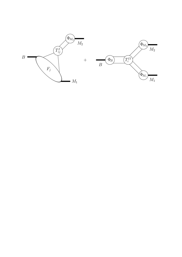
The second equation in (2.2) applies to decays into two light mesons, for which the spectator quark in the $B$ meson (in the following simply referred to as the “spectator quark”) can go to either of the final-state mesons. An example is the decay $B^{-}\to\pi^{0}K^{-}$. If the spectator quark can go only to one of the final-state mesons, as for example in $\bar{B}_{d}\to\pi^{+}K^{-}$, we call this meson $M_{1}$, and the second form-factor term on the right-hand side of (2.2) is absent. The formula simplifies when the spectator quark goes to a heavy meson (first equation in (2.2)), such as in $\bar{B}_{d}\to D^{+}\pi^{-}$. Then the second term in Fig. 1, which accounts for hard interactions with the spectator quark, can be dropped because it is power suppressed in the heavy-quark limit. In the opposite situation that the spectator quark goes to a light meson but the other meson is heavy, factorization does not hold, because the heavy meson is neither fast nor small and cannot be factorized from the $B\to M_{1}$ transition. Finally, notice that annihilation topologies do not appear in the factorization formula, since they do not contribute at leading order in the heavy-quark expansion.

Any hard interaction costs a power of $\alpha_{s}$. As a consequence, the hard-spectator term in the second formula in (2.2) is absent at order $\alpha_{s}^{0}$. Since at this order the functions $T^{I}_{ij}(u)$ are independent of $u$, the convolution integral results in the normalization of the meson distribution amplitude, and (2.2) reproduces naive factorization. The factorization formula allows us to compute radiative corrections to this result to all orders in $\alpha_{s}$. Further corrections are suppressed by powers of $\Lambda_{\rm QCD}/m_{b}$ in the heavy-quark limit.

The significance and usefulness of the factorization formula stems from the fact that the non-perturbative quantities appearing on the right-hand side of the two equations in (2.2) are much simpler than the original non-leptonic matrix elements on the left-hand side. This is because they either reflect universal properties of a single meson (light-cone distribution amplitudes) or refer only to a $B\to\mbox{meson}$ transition matrix element of a local current (form factors). While it is extremely difficult, if not impossible $\!{}^{{\bf?}}$, to compute the original matrix element $\langle M_{1}M_{2}|O_{i}|B\rangle$ in lattice QCD, form factors and light-cone distribution amplitudes are already being computed in this way, although with significant systematic errors at present. Alternatively, form factors can be obtained using data on semi-leptonic decays, and light-cone distribution amplitudes by comparison with other hard exclusive processes.

After having presented the most general form of the factorization formula, we will from now on restrict ourselves to the case of heavy-light final states. Then the (simpler) first formula in (2.2) applies, and only the first term shown in Fig. 1 is present at leading power.

2.3 Definition of non-perturbative parameters

The form factors $F_{j}^{B\to M}(q^{2})$ in (2.2) arise in the decomposition of current matrix elements of the form $\langle M(p^{\prime})|\bar{q}\Gamma b|\bar{B}(p)\rangle$, where $\Gamma$ can be any irreducible Dirac matrix that appears after contraction of the hard subgraph to a local vertex with respect to the $B\to M$ transition. We will often refer to the matrix element of the vector current evaluated between a $B$ meson and a pseudoscalar meson $P$, which is conventionally parameterized as

$$\langle P(p^{\prime})|\bar{q}\gamma^{\mu}b|\bar{B}(p)\rangle = F_{+}^{B\to P}(q^{2})\,(p^{\mu}+{p^{\prime}}^{\mu})$$ (4)

$$+ \Big{[}F_{0}^{B\to P}(q^{2})-F_{+}^{B\to P}(q^{2})\Big{]}\,\frac{m_{B}^{2}-m_{P}^{2}}{q^{2}}\,q^{\mu}\,,$$

where $q=p-p^{\prime}$, and $F_{+}^{B\to P}(0)=F_{0}^{B\to P}(0)$ at zero momentum transfer. Note that we write (2.2) in terms of physical form factors. In principle, Fig. 1 could be looked upon in two different ways. We could suppose that the region represented by $F_{j}$ accounts only for the soft contributions to the $B\to M_{1}$ form factor. The hard contributions to the form factor would then be considered as part of $T^{I}_{ij}$ (or as part of the second diagram). Performing this split-up would require that one understands the factorization of hard and soft contributions to the form factor. If $M_{1}$ is heavy, this amounts to matching the form factor onto a form factor defined in heavy-quark effective theory $\!{}^{{\bf?}}$. However, for a light meson $M_{1}$ the factorization of hard and soft contributions to the form factor is not yet completely understood. We bypass this problem by interpreting $F_{j}$ as the physical form factor, including hard and soft contributions. This avoids the above problem, and in addition has the advantage that the physical form factors are directly related to measurable quantities.

Light-cone distribution amplitudes play the same role for hard exclusive processes that parton distributions play for inclusive processes. As in the latter case, the leading-twist distribution amplitudes, which are the ones we need at leading power in the $1/m_{b}$ expansion, are given by two-particle operators with a certain helicity structure. The helicity structure is determined by the angular momentum of the meson and the fact that the spinor of an energetic quark has only two large components. The leading-twist light-cone distribution amplitudes for pseudoscalar mesons ($P$) and longitudinally polarized vector mesons ($V_{\parallel}$) with flavour content $(\bar{q}q^{\prime})$ are defined as

$$\langle P(q)|\bar{q}(y)_{\alpha}q^{\prime}(x)_{\beta}|0\rangle = \frac{if_{P}}{4}\,(\not\!q\gamma_{5})_{\beta\alpha}\int_{0}^{1}\!du\,e^{i(\bar{u}qx+uqy)}\,\Phi_{P}(u,\mu)\,,$$

$$\langle V_{\parallel}(q)|\bar{q}(y)_{\alpha}q^{\prime}(x)_{\beta}|0\rangle = -\frac{if_{V}}{4}\!\!\not\!q_{\beta\alpha}\int_{0}^{1}\!du\,e^{i(\bar{u}qx+uqy)}\,\Phi_{\parallel}(u,\mu)\,,$$ (5)

where $(x-y)^{2}=0$. We have suppressed the path-ordered exponentials that connect the two quark fields at different positions and make the light-cone operators gauge invariant. The equality sign is to be understood as “equal up to higher-twist terms”. It is also understood that the operators on the left-hand side are colour singlets. When convenient, we use the “bar”-notation $\bar{u}\equiv 1-u$. The parameter $\mu$ is the renormalization scale of the light-cone operators on the left-hand side. The distribution amplitudes are normalized as $\int_{0}^{1}du\,\Phi_{X}(u,\mu)=1$ with $X=P,V_{\parallel}$. One defines the asymptotic distribution amplitude as the limit in which the renormalization scale is sent to infinity. In this case

$$\Phi_{X}(u,\mu)\stackrel{{\scriptstyle\mu\to\infty}}{{=}}6u(1-u)\,.$$ (6)

The use of light-cone distribution amplitudes in non-leptonic $B$ decays requires justification, which we will provide in Sects. 3 and 4. The decay amplitude for a $B$ decay into a heavy-light final state is then calculated by assigning momenta $uq$ and $\bar{u}q$ to the quark and antiquark in the outgoing light meson (with momentum $q$), writing down the on-shell amplitude in momentum space, and performing the replacement

$$\bar{u}_{\alpha a}(uq)\,\Gamma(u,\dots)_{\alpha\beta,ab}v_{\beta b}(\bar{u}q)\to\frac{if_{P}}{4N_{c}}\int_{0}^{1}\!du\,\Phi_{P}(u)\,(\not\!q\gamma_{5})_{\beta\alpha}\,\Gamma(u,\dots)_{\alpha\beta,aa}$$ (7)

for pseudoscalars and, with obvious modifications, for vector mesons. (Even when working with light-cone distribution amplitudes it is not always justified to perform the collinear approximation on the external quark and antiquark lines right away. One may have to keep the transverse components of the quark and antiquark momenta until after some operations on the amplitude have been carried out. However, these subtleties do not concern calculations at leading-twist order.)

3 Arguments for factorization

In this section we provide the basic power-counting arguments that lead to the factorized structure shown in (2.2). We do so by analyzing qualitatively the hard, soft and collinear contributions to the simplest Feynman diagrams.

3.1 Preliminaries and power counting

For concreteness, we label the charm meson which picks up the spectator quark by $M_{1}=D^{+}$ and assign momentum $p^{\prime}$ to it. The light meson is labeled $M_{2}=\pi^{-}$ and assigned momentum $q=E\,n_{+}$, where $E$ is the pion energy in the $B$ rest frame, and $n_{\pm}=(1,0,0,\pm 1)$ are four-vectors on the light-cone. At leading power, we neglect the mass of the light meson.

The simplest diagrams that we can draw for a non-leptonic decay amplitude assign a quark and antiquark to each meson. We choose the quark and antiquark momenta in the pion as

$$l_{q}=uq+l_{\perp}+\frac{\vec{l}_{\perp}^{\,2}}{4uE}\,n_{-}\,,\qquad l_{\bar{q}}=\bar{u}q-l_{\perp}+\frac{\vec{l}_{\perp}^{\,2}}{4\bar{u}E}\,n_{-}\,.$$ (8)

Note that $q\neq l_{q}+l_{\bar{q}}$, but the off-shellness $(l_{q}+l_{\bar{q}})^{2}$ is of the same order as the light meson mass, which we can neglect at leading power. A similar decomposition (with longitudinal momentum fraction $v$ and transverse momentum $l_{\perp}^{\prime}$) is used for the charm meson.

To prove the factorization formula (2.2) for the case of heavy-light final states, one has to show that:

• There is no leading (in powers of $\Lambda_{\rm QCD}/m_{b}$) contribution to the amplitude from the endpoint regions $u\sim\Lambda_{\rm QCD}/m_{b}$ and $\bar{u}\sim\Lambda_{\rm QCD}/m_{b}$.

• One can set $l_{\perp}=0$ in the amplitude (more generally, expand the amplitude in powers of $l_{\perp}$) after collinear subtractions, which can be absorbed into the pion wave function. This, together with i), guarantees that the amplitude is legitimately expressed in terms of the light-cone distribution amplitudes of pion.

• The leading contribution comes from $\bar{v}\sim\Lambda_{\rm QCD}/m_{b}$ (the region where the spectator quark enters the charm meson as a soft parton), which guarantees the absence of a hard spectator interaction term.

• After subtraction of infrared contributions corresponding to the light-cone distribution amplitude and the form factor, the leading contributions to the amplitude come only from internal lines with virtuality that scales with $m_{b}$.

• Non-valence Fock states are non-leading.

The requirement that after subtractions virtualities should be large is obvious to guarantee the infrared finiteness of the hard-scattering functions $T^{I}_{ij}$. Let us comment on setting transverse momenta in the wave functions to zero and on endpoint contributions. Neglecting transverse momenta requires that we count them as order $\Lambda_{\rm QCD}$ when comparing terms of different magnitude in the scattering amplitude. This conforms to our intuition and the assumption of the parton model, that intrinsic transverse momenta are limited to hadronic scales. However, in QCD transverse momenta are not limited, but logarithmically distributed up to the hard scale. The important point is that contributions that violate the starting assumption of limited transverse momentum can be absorbed into the universal light-cone distribution amplitudes. The statement that transverse momenta can be counted of order $\Lambda_{\rm QCD}$ is to be understood after these subtractions have been performed.

The second comment concerns endpoint contributions in the convolution integrals over longitudinal momentum fractions. These contributions are dangerous, because we may be able to demonstrate the infrared safety of the hard-scattering amplitude under assumption of generic $u$ and independent of the shape of the meson distribution amplitude, but for $u\to 0$ or $u\to 1$ a propagator that was assumed to be off-shell approaches the mass-shell. If such a contribution were of leading power, we would not expect the perturbative calculation of the hard-scattering functions to be reliable.

Estimating endpoint contributions requires knowledge of the endpoint behaviour of the light-cone distribution amplitude. Since it enters the factorization formula at a renormalization scale of order $m_{b}$, we can use the asymptotic form (6) to estimate the endpoint contribution. (More generally, we only have to assume that the distribution amplitude at a given scale has the same endpoint behaviour as the asymptotic amplitude. This is generally the case, unless there is a conspiracy of terms in the Gegenbauer expansion of the distribution amplitude. If such a conspiracy existed at some scale, it would be destroyed by evolving the distribution amplitude to a different scale.) We count a light-meson distribution amplitude as order $\Lambda_{\rm QCD}/m_{b}$ in the endpoint region (defined as the region the quark or antiquark momentum is of order $\Lambda_{\rm QCD}$), and order $1$ away from the endpoint, i.e. (for $X=P,V_{\parallel}$)

$$\Phi_{X}(u)\sim\left\{\begin{array}[]{cl}1\,;&\quad\mbox{generic $u$,}\\[2.84544pt] \Lambda_{\rm QCD}/m_{b}\,;&\quad u,\,\bar{u}\sim\Lambda_{\rm QCD}/m_{b}.\end{array}\right.$$ (9)

Note that the endpoint region has a size of order $\Lambda_{\rm QCD}/m_{b}$, so that the endpoint suppression is $\sim(\Lambda_{\rm QCD}/m_{b})^{2}$. This suppression has to be weighted against potential enhancements of the partonic amplitude when one of the propagators approaches the mass shell. The counting for $B$ mesons, or heavy mesons in general, is different. Naturally, the heavy quark carries almost all of the meson momentum, and hence we count

$$\Phi_{B}(\xi)\sim\left\{\begin{array}[]{cl}m_{b}/\Lambda_{\rm QCD}\,;&\quad\xi\sim\Lambda_{\rm QCD}/m_{b},\\[2.84544pt] 0\,;&\quad\xi\sim 1.\end{array}\right.$$ (10)

The zero probability for a light spectator with momentum of order $m_{b}$ must be understood as a boundary condition for the wave function renormalized at a scale much below $m_{b}$. There is a small probability for hard fluctuations that transfer large momentum to the spectator. This “hard tail” is generated by evolution of the wave function from a hadronic scale to a scale of order $m_{b}$. If we assume that the initial distribution at the hadronic scale falls sufficiently rapidly for $\xi\gg\Lambda_{\rm QCD}/m_{b}$, this remains true after evolution. We shall assume a sufficiently fast fall-off, so that, for the purposes of power counting, the probability that the spectator-quark momentum is of order $m_{b}$ can be set to zero. The same counting applies to the $D$ meson. (Despite the fact that the charm meson has momentum of order $m_{b}$, we do not need to distinguish the rest frames of $B$ and $D$ for the purpose of power counting, because the two frames are not connected by a parametrically large boost. In other words, the components of the spectator quark in the $D$ meson are still of order $\Lambda_{\rm QCD}$.)

3.2 The $B\to D$ form factor

We now demonstrate that the $B\to D$ form factor receives a leading contribution from soft gluon exchange. This implies that a non-leptonic decay cannot be treated completely in the hard-scattering picture, and so the form factor should enter the factorization formula as a non-perturbative quantity.

Figure 2: Leading contributions to the $B\to D$ form factor in the hard-scattering approach. The dashed line represents the weak current. The two lines to the left belong to the $B$ meson, the ones to the right to the recoiling charm meson.

Consider the diagrams shown in Fig. 2. When the exchanged gluon is hard the spectator quark in the final state has momentum of order $m_{b}$. But according to the counting rule (10) this configuration has no overlap with the $D$-meson wave function. On the other hand, there is no suppression for soft gluons in Fig. 2. It follows that the dominant behaviour of the $B\to D$ form factor in the heavy-quark limit is given by soft processes.

Because of this argument, we can exploit the heavy-quark symmetries to determine how the form factor scales in the heavy-quark limit. The well-known result is that the form factor scales like a constant (modulo logarithms), since it is equal to one at zero velocity transfer and independent of $m_{b}$ as long as the Lorentz boost that connects the $B$ and $D$ rest frames is of order 1. The same conclusion follows from the power-counting rules for light-cone wave functions. To see this, we represent the form factor by an overlap integral of wave functions (not integrated over transverse momentum),

$$F_{+,0}^{B\to D}(0)\sim\int\frac{d\xi d^{2}k_{\perp}}{16\pi^{3}}\,\Psi_{B}(\xi,k_{\perp})\,\Psi_{D}(\xi^{\prime}(\xi),k_{\perp})\,,$$ (11)

where $\xi^{\prime}(\xi)$ is fixed by kinematics, and we have set $q^{2}=0$ for simplicity. The probability of finding the $B$ meson in its valence Fock state is of order 1 in the heavy-quark limit, i.e.

$$\int\frac{d\xi d^{2}k_{\perp}}{16\pi^{3}}\,|\Psi_{B,D}(\xi,k_{\perp})|^{2}\sim 1\,.$$ (12)

Counting $k_{\perp}\sim\Lambda_{\rm QCD}$ and $d\xi\sim\Lambda_{\rm QCD}/m_{b}$, we deduce that $\Psi_{B}(\xi,k_{\perp})\sim m_{b}^{1/2}/\Lambda_{\rm QCD}^{3/2}$. From (11), we then obtain the scaling law $F_{+,0}^{B\to D}(0)\sim 1$, in agreement with the prediction of heavy-quark symmetry.

The representation (11) of the form factor as an overlap of wave functions for the two-particle Fock state of the heavy meson is not rigorous, because there is no reason to assume that the contribution from higher Fock states with additional soft gluons is suppressed. The consistency with the estimate based on heavy-quark symmetry shows that these additional contributions are not larger than the two-particle contribution.

3.3 Non-leptonic decay amplitudes

We now turn to a qualitative discussion of the lowest-order and one-gluon exchange diagrams that could contribute to the hard-scattering kernels $T^{I}_{ij}(u)$ in (2.2). In the figures which follow, the two lines directed upwards represent $\pi^{-}$, the lines on the left represent $\bar{B}_{d}$, and the lines on the right represent $D^{+}$.

Lowest-order diagram

Figure 3: Leading-order contribution to the hard-scattering kernels $T^{I}_{ij}(u)$. The weak decay of the $b$ quark through a four-fermion operator is represented by the black square.

There is a single diagram with no hard gluon interactions shown in Fig. 3. According to (10) the spectator quark is soft, and since it does not undergo a hard interaction it is absorbed as a soft quark by the recoiling meson. This is evidently a contribution to the left-hand diagram of Fig. 1, involving the $B\to D$ form factor. The hard subprocess in Fig. 3 is just given by the insertion of a four-fermion operator, and hence it does not depend on the longitudinal momentum fraction $u$ of the two quarks that form the emitted $\pi^{-}$. Consequently, the lowest-order contribution to $T_{ij}^{I}(u)$ in (2.2) is independent of $u$, and the $u$-integral reduces to the normalization condition for the pion distribution amplitude. The result is, not surprisingly, that the factorization formula reproduces the result of naive factorization if we neglect gluon exchange. Note that the physical picture underlying this lowest-order process is that the spectator quark (which is part of the $B\to D$ form factor) is soft. If this is the case, the hard-scattering approach misses the leading contribution to the non-leptonic decay amplitude.

Putting together all factors relevant to power counting, we find that in the heavy-quark limit the decay amplitude for a decay into a heavy-light final state (in which the spectator quark is absorbed by the heavy meson) scales as

$${\cal A}(\bar{B}_{d}\to D^{+}\pi^{-})\sim G_{F}m_{b}^{2}\,F^{B\to D}(0)\,f_{\pi}\sim G_{F}m_{b}^{2}\,\Lambda_{\rm QCD}\,.$$ (13)

Other contributions must be compared with this scaling rule.

Factorizable diagrams

In order to justify naive factorization as the leading term in an expansion in $\alpha_{s}$ and $\Lambda_{\rm QCD}/m_{b}$, we must show that radiative corrections are either suppressed in one of these two parameters, or already contained in the definition of the form factor and the pion decay constant. Consider the graphs shown in Fig. 4. The first three diagrams are part of the form factor and do not contribute to the hard-scattering kernels. Since the first and third diagrams contain leading contributions from the region in which the gluon is soft, they should not be considered as corrections to Fig. 3. However, this is of no consequence since these soft contributions are absorbed into the physical form factor.

Figure 4: Diagrams at order $\alpha_{s}$ that need not be calculated.

The fourth diagram in Fig. 4 is also factorizable. In general, this graph would split into a hard contribution and a contribution to the evolution of the pion distribution amplitude. However, as the leading-order diagram in Fig. 3 involves only the normalization integral of the pion distribution amplitude, the sum of the fourth diagram in Fig. 4 and the wave-function renormalization of the quarks in the emitted pion vanishes. In other words, these diagrams would renormalize the $(\bar{u}d)$ light-quark current, which however is conserved.

“Non-factorizable” vertex corrections

We now begin the analysis of “non-factorizable” diagrams, i.e. diagrams containing gluon exchanges that cannot be associated with the $B\to D$ form factor or the pion decay constant. At order $\alpha_{s}$, these diagrams can be divided into three groups: vertex corrections, hard spectator interactions, and annihilation diagrams.

The vertex corrections shown in Fig. 5 violate the naive factorization ansatz (2). One of the key observations made in $\!{}^{{\bf?},{\bf?}}$ is that these diagrams are calculable nonetheless. Let us summarize the argument here, postponing the explicit evaluation of these diagrams to Sect. 4. The statement is that the vertex-correction diagrams form an order-$\alpha_{s}$ contribution to the hard-scattering kernels $T^{I}_{ij}(u)$. To demonstrate this, we have to show that: i) The transverse momentum of the quarks that form the pion can be neglected at leading power, i.e. the two momenta in (8) can be approximated by $uq$ and $\bar{u}q$, respectively. This guarantees that only a convolution in the longitudinal momentum fraction $u$ appears in the factorization formula. ii) The contribution from the soft-gluon region and gluons collinear to the direction of the pion is power suppressed. In practice, this means that the sum of these diagrams cannot contain any infrared divergences at leading power in $\Lambda_{\rm QCD}/m_{b}$.

Figure 5: “Non-factorizable” vertex corrections.

Neither of the two conditions holds true for any of the four diagrams individually, as each of them separately contains collinear and infrared divergences. As will be shown in detail later, the infrared divergences cancel when one sums over the gluon attachments to the two quarks comprising the emission pion ((a+b), (c+d) in Fig. 5). This cancellation is a technical manifestation of Bjorken’s colour-transparency argument $\!{}^{{\bf?}}$, stating that soft gluon interactions with the emitted colour-singlet $(\bar{u}d)$ pair are suppressed because they interact with the colour dipole moment of the compact light-quark pair. Collinear divergences cancel after summing over gluon attachments to the $b$ and $c$ quark lines ((a+c), (b+d) in Fig. 5). Thus the sum of the four diagrams (a–d) involves only hard gluon exchange at leading power. Because the hard gluons transfer large momentum to the quarks that form the emission pion, the hard-scattering factor now results in a non-trivial convolution with the pion distribution amplitude. “Non-factorizable” contributions are therefore non-universal, i.e. they depend on the quantum numbers of the final-state mesons.

Note that the colour-transparency argument, and hence the cancellation of soft gluon effects, applies only if the $(\bar{u}d)$ pair is compact. This is not the case if the emitted pion is formed in a very asymmetric configuration, in which one of the quarks carries almost all of the pion momentum. Since the probability for forming a pion in such an endpoint configuration is of order $(\Lambda_{\rm QCD}/m_{b})^{2}$, they could become important only if the hard-scattering amplitude favoured the production of these asymmetric pairs, i.e. if $T^{I}_{ij}\sim 1/u^{2}$ for $u\to 0$ (or $T^{I}_{ij}\sim 1/\bar{u}^{2}$ for $u\to 1$). However, we will see that such strong endpoint singularities in the hard-scattering amplitude do not occur.

To complete the argument, we have to show that all other types of contributions to the non-leptonic decay amplitudes are power suppressed in the heavy-quark limit. This includes interactions with the spectator quark, weak annihilation graphs, and contributions from higher Fock components of the meson wave functions. This will be done in Sect. 5. In summary, then, for hadronic $B$ decays into a light emitted and a heavy recoiling meson the first factorization formula in (2.2) holds. At order $\alpha_{s}$, the hard-scattering kernels $T^{I}_{ij}(u)$ are computed from the diagrams shown in Figs. 3 and 5. Naive factorization follows when one neglects all corrections of order $\Lambda_{\rm QCD}/m_{b}$ and $\alpha_{s}$. The factorization formula allows us to compute systematically corrections to higher order in $\alpha_{s}$, but still neglects power corrections.

3.4 Remarks on final-state interactions

Some of the loop diagrams entering the calculation of the hard-scattering kernels have imaginary parts, which contribute to the strong rescattering phases. It follows from our discussion that these imaginary parts are of order $\alpha_{s}$ or $\Lambda_{\rm QCD}/m_{b}$. This demonstrates that strong phases vanish in the heavy-quark limit (unless the real parts of the amplitudes are also suppressed). Since this statement goes against the folklore that prevails from the present understanding of this issue, and since the subject of final-state interactions (and of strong-interaction phases in particular) is of paramount importance for the interpretation of CP-violating observables, a few additional remarks are in order.

Final-state interactions are usually discussed in terms of intermediate hadronic states. This is suggested by the unitarity relation (taking $B\to\pi\pi$ for definiteness)

$$\mbox{Im}\,{\cal A}_{B\to\pi\pi}\sim\sum_{n}{\cal A}_{B\to n}\,{\cal A}_{n\to\pi\pi}^{*}\,,$$ (14)

where $n$ runs over all hadronic intermediate states. We can also interpret the sum in (14) as extending over intermediate states of partons. The partonic interpretation is justified by the dominance of hard rescattering in the heavy-quark limit. In this limit, the number of physical intermediate states is arbitrarily large. We may then argue on the grounds of parton–hadron duality that their average is described well enough (up to $\Lambda_{\rm QCD}/m_{b}$ corrections, say) by a partonic calculation. This is the picture implied by (2.2). The hadronic language is in principle exact. However, the large number of intermediate states makes it intractable to observe systematic cancellations, which usually occur in an inclusive sum over hadronic intermediate states.

A particular contribution to the right-hand side of (14) is elastic rescattering ($n=\pi\pi$). The energy dependence of the total elastic $\pi\pi$-scattering cross section is governed by soft pomeron behaviour. Hence the strong-interaction phase of the $B\to\pi\pi$ amplitude due to elastic rescattering alone increases slowly in the heavy-quark limit $\!{}^{{\bf?}}$. On general grounds, it is rather improbable that elastic rescattering gives an appropriate representation of the imaginary part of the decay amplitude in the heavy-quark limit. This expectation is also borne out in the framework of Regge behaviour, as discussed in $\!{}^{{\bf?}}$, where the importance (in fact, dominance) of inelastic rescattering was emphasized. However, this discussion left open the possibility of soft rescattering phases that do not vanish in the heavy-quark limit, as well as the possibility of systematic cancellations, for which the Regge approach does not provide an appropriate theoretical framework.

Eq. (2.2) implies that such systematic cancellations do occur in the sum over all intermediate states $n$. It is worth recalling that similar cancellations are not uncommon for hard processes. Consider the example of $e^{+}e^{-}\to\,$hadrons at large energy $q$. While the production of any hadronic final state occurs on a time scale of order $1/\Lambda_{\rm QCD}$ (and would lead to infrared divergences if we attempted to describe it using perturbation theory), the inclusive cross section given by the sum over all hadronic final states is described very well by a $(q\bar{q})$ pair that lives over a short time scale of order $1/q$. In close analogy, while each particular hadronic intermediate state $n$ in (14) cannot be described partonically, the sum over all intermediate states is accurately represented by a $(q\bar{q})$ fluctuation of small transverse size of order $1/m_{b}$. Because the $(q\bar{q})$ pair is small, the physical picture of rescattering is very different from elastic $\pi\pi$ scattering.

In perturbation theory, the pomeron is associated with two-gluon exchange. The analysis of two-loop contributions to the non-leptonic decay amplitude in $\!{}^{{\bf?}}$ shows that the soft and collinear cancellations that guarantee the partonic interpretation of rescattering extend to two-gluon exchange. Hence, the soft final-state interactions are again subleading as required by the validity of (2.2). As far as the hard rescattering contributions are concerned, two-gluon exchange plus ladder graphs between a compact $(q\bar{q})$ pair with energy of order $m_{b}$ and transverse size of order $1/m_{b}$ and the other pion does not lead to large logarithms, and hence there is no possibility to construct the (hard) pomeron. Note the difference with elastic vector-meson production through a virtual photon, which also involves a compact $(q\bar{q})$ pair. However, in this case one considers $s\gg Q^{2}$, where $\sqrt{s}$ is the photon–proton center-of-mass energy and $Q$ the virtuality of the photon. This implies that the $(q\bar{q})$ fluctuation is born long before it hits the proton. It is this difference of time scales, non-existent in non-leptonic $B$ decays, that permits pomeron exchange in elastic vector-meson production in $\gamma^{*}p$ collisions.

4 $B\to D\pi$: Factorization at one-loop order

We now present a more detailed treatment of the exclusive decays $\bar{B}_{d}\to D^{(*)+}L^{-}$, where $L$ is a light meson. We illustrate explicitly how factorization emerges at one-loop order and compute the hard-scattering kernels $T_{ij}^{I}(u)$ in the factorization formula (2.2). For each final state $f$, we express the decay amplitudes in terms of parameters $a_{1}(f)$ defined in analogy with similar parameters used in the literature on naive factorization.

4.1 Effective Hamiltonian and decay topologies

The effective Hamiltonian for $B\to D\pi$ is

$${\cal H}_{\rm eff}=\frac{G_{F}}{\sqrt{2}}\,V^{*}_{ud}V_{cb}\,(C_{0}O_{0}+C_{8}O_{8})\,.$$ (15)

We choose to write the two independent four-quark operators in the singlet–octet basis

$$O_{0} = \bar{c}\gamma^{\mu}(1-\gamma_{5})b\,\bar{d}\gamma_{\mu}(1-\gamma_{5})u\,,$$

$$O_{8} = \bar{c}\gamma^{\mu}(1-\gamma_{5})T^{A}b\,\bar{d}\gamma_{\mu}(1-\gamma_{5})T^{A}u\,,$$ (16)

rather than in the more conventional basis of $O_{1}$ and $O_{2}$. The Wilson coefficients $C_{0}$ and $C_{8}$ describe the exchange of hard gluons with virtualities between the high-energy matching scale $M_{W}$ and a renormalization scale $\mu$ of order $m_{b}$. (These coefficients are related to the ones of the standard basis by $C_{0}=C_{1}+C_{2}/3$ and $C_{8}=2C_{2}$.) They are known at next-to-leading order in renormalization-group improved perturbation theory and are given by $\!{}^{{\bf?}}$

$$C_{0}=\frac{N_{c}+1}{2N_{c}}\,C_{+}+\frac{N_{c}-1}{2N_{c}}\,C_{-}\,,\qquad C_{8}=C_{+}-C_{-}\,,$$ (17)

where

$$C_{\pm}(\mu)=\left(1+\frac{\alpha_{s}(\mu)}{4\pi}\,B_{\pm}\right)\,\bar{C}_{\pm}(\mu)\,,\qquad B_{\pm}=\pm\frac{N_{c}\mp 1}{2N_{c}}\,B\,,$$ (18)

and

$$\bar{C}_{\pm}(\mu)=\left[\frac{\alpha_{s}(M_{W})}{\alpha_{s}(\mu)}\right]^{d_{\pm}}\left[1+\frac{\alpha_{s}(M_{W})-\alpha_{s}(\mu)}{4\pi}\,S_{\pm}\right]\,.$$ (19)

For $N_{c}=3$ and $f=5$, we have $d_{+}=\frac{6}{25}$ and $d_{-}=-\frac{12}{25}$, as well as $S_{+}=\frac{6473}{3174}$ and $S_{-}=-\frac{9371}{1587}$. The scheme dependence of the Wilson coefficients at next-to-leading order is parameterized by the coefficient $B$ in (18). We note that $B_{\rm NDR}=11$ in the naive dimensional regularization (NDR) scheme with anticommuting $\gamma_{5}$, and $B_{\rm HV}=7$ in the ‘t Hooft–Veltman (HV) scheme. We will demonstrate below that the scale and scheme dependence of the Wilson coefficients is canceled by a corresponding scale and scheme dependence of the hadronic matrix elements of the operators $O_{0}$ and $O_{8}$.

Before continuing with a discussion of these matrix elements, it is useful to consider the flavour structure for the various contributions to $B\to D\pi$ decays. The possible quark-level topologies are depicted in Fig. 6. In the terminology generally adopted for two-body non-leptonic decays, the decays $\bar{B}_{d}\to D^{+}\pi^{-}$, $\bar{B}_{d}\to D^{0}\pi^{0}$ and $B^{-}\to D^{0}\pi^{-}$ are referred to as class-I, class-II and class-III, respectively $\!{}^{{\bf?}}$. In $\bar{B}_{d}\to D^{+}\pi^{-}$ and $B^{-}\to D^{0}\pi^{-}$ decays the pion can be directly created from the weak current. We call this a class-I contribution, following the above terminology. In addition, in the case of $\bar{B}_{d}\to D^{+}\pi^{-}$ there is a contribution from weak annihilation, and a class-II amplitude contributes to $B^{-}\to D^{0}\pi^{-}$. The important point is that the spectator quark goes into the light meson in the case of the class-II amplitude. This amplitude is suppressed in the heavy-quark limit, as is the annihilation amplitude. It follows that the amplitude for $\bar{B}_{d}\to D^{0}\pi^{0}$, receiving only class-II and annihilation contributions, is subleading compared with $\bar{B}_{d}\to D^{+}\pi^{-}$ and $B^{-}\to D^{0}\pi^{-}$, which are dominated by the class-I topology.

Figure 6: Basic quark-level topologies for $B\to D\pi$ decays ($q=u$, $d$): (a) class-I, (b) class-II, (c) weak annihilation. $\bar{B}_{d}\to D^{+}\pi^{-}$ receives contributions from (a) and (c), $\bar{B}_{d}\to D^{0}\pi^{0}$ from (b) and (c), and $B^{-}\to D^{0}\pi^{-}$ from (a) and (b). Only (a) contributes in the heavy-quark limit.

We shall use the one-loop analysis for $\bar{B}_{d}\to D^{+}\pi^{-}$ as a concrete example to illustrate explicitly the various steps involved in establishing the factorization formula. Most of the arguments given below are standard from the theory of hard exclusive processes involving light hadrons $\!{}^{{\bf?}}$. However, it is instructive to repeat these arguments in the context of $B$ decays.

4.2 Soft and collinear cancellations at one-loop order

In order to demonstrate the property of factorization for the decay $\bar{B}_{d}\to D^{+}\pi^{-}$, we now analyze the “non-factorizable” one-gluon exchange contributions shown in Fig. 5 in some detail. We consider the leading, valence Fock state of the emitted pion. This is justified since higher Fock components only give power-suppressed contributions to the decay amplitude in the heavy-quark limit (as demonstrated later). For the purpose of our discussion, the valence Fock state of the pion can be written as

$$|\pi(q)\rangle=\int\frac{du}{\sqrt{u\bar{u}}}\,\frac{d^{2}l_{\perp}}{16\pi^{3}}\,\frac{1}{\sqrt{2N_{c}}}\left(a^{\dagger}_{\uparrow}(l_{q})\,b^{\dagger}_{\downarrow}(l_{\bar{q}})-a^{\dagger}_{\downarrow}(l_{q})\,b^{\dagger}_{\uparrow}(l_{\bar{q}})\right)|0\rangle\,\Psi(u,\vec{l}_{\perp})\,,$$ (20)

where $a^{\dagger}_{s}$ ($b^{\dagger}_{s}$) denotes the creation operator for a quark (antiquark) in a state with spin $s=\uparrow$ or $s=\downarrow$, and we have suppressed colour indices. The wave function $\Psi(u,\vec{l}_{\perp})$ is defined as the amplitude for the pion to be composed of two on-shell quarks, characterized by longitudinal momentum fraction $u$ and transverse momentum $l_{\perp}$. The on-shell momenta of the quark and antiquark are chosen as in (8). For the purpose of power counting, $l_{\perp}\sim\Lambda_{\rm QCD}\ll E\sim m_{b}$. Note that the invariant mass of the valence state is $(l_{q}+l_{\bar{q}})^{2}=\vec{l}^{\,2}_{\perp}/(u\bar{u})$, which is of order $\Lambda^{2}_{\rm QCD}$ and hence negligible in the heavy-quark limit unless $u$ is in the vicinity of the endpoints $u=0$ or 1. In this case, the invariant mass of the quark–antiquark pair becomes large, and the valence Fock state is no longer a valid representation of the pion. However, in the heavy-quark limit the dominant contributions to the decay amplitude come from configurations where both partons are hard ($u$ and $\bar{u}$ both of order 1), and so the two-particle Fock state yields a consistent description. We will provide an explicit consistency check of this important feature later on.

As a next step, we write down the amplitude

$$\langle\pi(q)|u(0)_{\alpha}\bar{d}(y)_{\beta}|0\rangle=\int\!du\,\frac{d^{2}l_{\perp}}{16\pi^{3}}\,\frac{1}{\sqrt{2N_{c}}}\,\Psi^{*}(u,\vec{l}_{\perp})\,(\gamma_{5}\!\not\!q)_{\alpha\beta}\,e^{il_{q}\cdot y}\,,$$ (21)

which appears as an ingredient of the $B\to D\pi$ matrix element. It is now straightforward to obtain the one-gluon exchange contribution to the $B\to D\pi$ matrix element of the operator $O_{8}$. For the sum of the four diagrams in Fig. 5, we find

$$\langle D^{+}\pi^{-}|O_{8}|\bar{B}_{d}\rangle_{\rm 1\mbox{-}gluon} =$$

$$ig_{s}^{2}\frac{C_{F}}{2}\!\int\!\frac{d^{4}k}{(2\pi)^{4}}\,\langle D^{+}|\bar{c}A_{1}(k)b|\bar{B}_{d}\rangle\,\frac{1}{k^{2}}\!\int^{1}_{0}\!du\,\frac{d^{2}l_{\perp}}{16\pi^{3}}\,\frac{\Psi^{*}(u,\vec{l}_{\perp})}{\sqrt{2N_{c}}}\,{\rm tr}[\gamma_{5}\!\not\!qA_{2}(l_{q},l_{\bar{q}},k)]\,,$$

where

$$A_{1}(k) = \frac{\gamma^{\lambda}(\not\!p_{c}-\not\!k+m_{c})\Gamma}{2p_{c}\cdot k-k^{2}}-\frac{\Gamma(\not\!p_{b}+\not\!k+m_{b})\gamma^{\lambda}}{2p_{b}\cdot k+k^{2}}\,,$$

$$A_{2}(l_{q},l_{\bar{q}},k) = \frac{\Gamma(\not\!l_{\bar{q}}+\not\!k)\gamma_{\lambda}}{2l_{\bar{q}}\cdot k+k^{2}}-\frac{\gamma_{\lambda}(\not\!l_{q}+\not\!k)\Gamma}{2l_{q}\cdot k+k^{2}}\,.$$ (23)

Here $\Gamma=\gamma^{\mu}(1-\gamma_{5})$, and $p_{b}$, $p_{c}$ are the momenta of the $b$- and $c$-quark, respectively. There is no correction to the matrix element of $O_{0}$ at order $\alpha_{s}$, because in this case the $(d\bar{u})$ pair is necessarily in a colour-octet configuration and cannot form a pion.

In (4.2) the pion wave function $\Psi(u,l_{\perp})$ appears separated from the $B\to D$ transition. This is merely a reflection of the fact that we have represented the pion state in the form shown in (20). It does not, by itself, imply factorization, since the right-hand side of (4.2) still involves non-trivial integrations over $\vec{l}_{\perp}$ and the gluon momentum $k$, and long- and short-distance contributions are not yet disentangled. In order to prove factorization, we need to show that the integral over $k$ receives only subdominant contributions from the region of small $k^{2}$. This is equivalent to showing that the integral over $k$ does not contain infrared divergences at leading power in $\Lambda_{\rm QCD}/m_{b}$.

To demonstrate infrared finiteness of the one-loop integral

$$J\equiv\int\!d^{4}k\,\frac{1}{k^{2}}\,A_{1}(k)\otimes A_{2}(l_{q},l_{\bar{q}},k)$$ (24)

at leading power, the heavy-quark limit and the corresponding large light-cone momentum of the pion are again essential. First note that when $k$ is of order $m_{b}$, $J\sim 1$ by dimensional analysis. Potential infrared divergences could arise when $k$ is soft or collinear to the pion momentum $q$. We need to show that the contributions from these regions are power suppressed. (Note that we do not need to show that $J$ is infrared finite. It is enough that logarithmic divergences have coefficients that are power suppressed.)

We treat the soft region first. Here all components of $k$ become small simultaneously, which we describe by scaling $k\sim\lambda$. Counting powers of $\lambda$ ($d^{4}k\sim\lambda^{4}$, $1/k^{2}\sim\lambda^{-2}$, $1/p\cdot k\sim\lambda^{-1}$) reveals that each of the four diagrams in Fig. 5, corresponding to the four terms in the product in (24), is logarithmically divergent. However, because $k$ is small the integrand can be simplified. For instance, the second term in $A_{2}$ can be approximated as

$$\frac{\gamma_{\lambda}(\not\!l_{q}+\not\!k)\Gamma}{2l_{q}\cdot k+k^{2}}=\frac{\gamma_{\lambda}(\!u\not\!q+\not\!l_{\perp}+\frac{\vec{l}^{2}_{\perp}}{4uE}\not\!n_{-}+\not\!k)\Gamma}{2uq\cdot k+2l_{\perp}\cdot k+\frac{\vec{l}^{2}_{\perp}}{2uE}n_{-}\cdot k+k^{2}}\simeq\frac{q_{\lambda}}{q\cdot k}\,\Gamma\,,$$ (25)

where we used that $\!\not\!q$ to the extreme left or right of an expression gives zero due to the on-shell condition for the external quark lines. We get exactly the same expression but with an opposite sign from the other term in $A_{2}$, and hence the soft divergence cancels out. More precisely, we find that the integral is infrared finite in the soft region when $l_{\perp}$ is neglected. When $l_{\perp}$ is not neglected, there is a divergence from soft $k$ which is proportional to $l^{2}_{\perp}/m_{b}^{2}\sim\Lambda^{2}_{\rm QCD}/m_{b}^{2}$. In either case, the soft contribution to $J$ is of order $\Lambda_{\rm QCD}/m_{b}$ or smaller and hence suppressed relative to the hard contribution. This corresponds to the standard soft cancellation mechanism, which is a technical manifestation of colour transparency.

Each of the four terms in (24) is also divergent when $k$ becomes collinear with the light-cone momentum $q$. This implies the scaling $k^{+}\sim\lambda^{0}$, $k_{\perp}\sim\lambda$, and $k^{-}\sim\lambda^{2}$. Then $d^{4}k\sim dk^{+}dk^{-}d^{2}k_{\perp}\sim\lambda^{4}$, and $q\cdot k=q^{+}k^{-}\sim\lambda^{2}$, $k^{2}=2k^{+}k^{-}+k^{2}_{\perp}\sim\lambda^{2}$. The divergence is again logarithmic, and it is thus sufficient to consider the leading behaviour in the collinear limit. Writing $k=\alpha q+\ldots$ we can now simplify the second term of $A_{2}$ as

$$\frac{\gamma_{\lambda}(\not\!l_{q}+\not\!k)\Gamma}{2l_{q}\cdot k+k^{2}}\simeq q_{\lambda}\,\frac{2(u+\alpha)\Gamma}{2l_{q}\cdot k+k^{2}}\,.$$ (26)

No simplification occurs in the denominator (in particular, $l_{\perp}$ cannot be neglected), but the important point is that the leading contribution is proportional to $q_{\lambda}$. Therefore, substituting $k=\alpha q$ into $A_{1}$ and using $q^{2}=0$, we obtain

$$q_{\lambda}A_{1}\simeq\frac{\not\!q(\not\!p_{c}+m_{c})\Gamma}{2\alpha p_{c}\cdot q}-\frac{\Gamma(\not\!p_{b}+m_{b})\!\not\!q}{2\alpha p_{b}\cdot q}=0\,,$$ (27)

employing the equations of motion for the heavy quarks. Hence the collinear divergence cancels by virtue of the standard Ward identity.

This completes the proof of the absence of infrared divergences at leading power in the hard-scattering kernel for $\bar{B}_{d}\to D^{+}\pi^{-}$ to one-loop order. Similar cancellations are observed at higher orders. A complete proof of factorization at two-loop order can be found in $\!{}^{{\bf?}}$. Having established that the “non-factorizable” diagrams of Fig. 5 are dominated by hard gluon exchange (i.e. that the leading contribution to $J$ arises from $k$ of order $m_{b}$), we may now use the fact that $|\vec{l}_{\perp}|\ll E$ to expand $A_{2}$ in powers of $|\vec{l}_{\perp}|/E$. To leading order the expansion simply reduces to neglecting $l_{\perp}$ altogether, which implies $l_{q}=uq$ and $l_{\bar{q}}=\bar{u}q$ in (8). As a consequence, we may perform the $l_{\perp}$ integration in (4.2) over the pion distribution amplitude. Defining

$$\int\frac{d^{2}l_{\perp}}{16\pi^{3}}\,\frac{\Psi^{*}(u,\vec{l}_{\perp})}{\sqrt{2N_{c}}}\equiv\frac{if_{\pi}}{4N_{c}}\,\Phi_{\pi}(u)\,,$$ (28)

the matrix element of $O_{8}$ in (4.2) becomes

$$\langle D^{+}\pi^{-}|O_{8}|\bar{B}_{d}\rangle_{\rm 1\mbox{-}gluon} =$$

$$-g_{s}^{2}\,\frac{C_{F}}{8N_{c}}\int\frac{d^{4}k}{(2\pi)^{4}}\,\langle D^{+}|\bar{c}A_{1}(k)b|\bar{B}_{d}\rangle\,\frac{1}{k^{2}}\,f_{\pi}\!\int^{1}_{0}\!du\,\Phi_{\pi}(u)\,{\rm tr}[\gamma_{5}\!\not\!qA_{2}(uq,\bar{u}q,k)]\,.$$

On the other hand, putting $y$ on the light-cone in (21) and comparing with (2.3), we see that the $l_{\perp}$-integrated wave function $\Phi_{\pi}(u)$ in (28) is precisely the light-cone distribution amplitude of the pion. This demonstrates the relevance of the light-cone wave function to the factorization formula. Note that the collinear approximation for the quark and antiquark momenta emerges automatically in the heavy-quark limit.

After the $k$ integral is performed, the expression (4.2) can be cast into the form

$$\langle D^{+}\pi^{-}|O_{8}|\bar{B}_{d}\rangle_{\rm 1\mbox{-}gluon}\sim F^{B\to D}(0)\int^{1}_{0}\!du\,T_{8}(u,z)\,\Phi_{\pi}(u)\,,$$ (30)

where $z=m_{c}/m_{b}$, $T_{8}(u,z)$ is the hard-scattering kernel, and $F^{B\to D}(0)$ the form factor that parameterizes the $\langle D^{+}|\bar{c}[\dots]b|\bar{B}_{d}\rangle$ matrix element. Because of the absence of soft and collinear infrared divergences in the gluon exchange between the $(\bar{c}b)$ and $(\bar{d}u)$ currents, the hard-scattering kernel $T_{8}$ is calculable in QCD perturbation theory.

4.3 Matrix elements at next-to-leading order

We now compute these hard-scattering kernels explicitly to order $\alpha_{s}$. The effective Hamiltonian (15) can be written as

$${\cal H}_{\rm eff} = \frac{G_{F}}{\sqrt{2}}V^{*}_{ud}V_{cb}\Bigg{\{}\left[\!\frac{N_{c}+1}{2N_{c}}\bar{C}_{+}(\mu)+\frac{N_{c}-1}{2N_{c}}\bar{C}_{-}(\mu)+\frac{\alpha_{s}(\mu)}{4\pi}\,\frac{C_{F}}{2N_{c}}\,BC_{8}(\mu)\!\right]\!O_{0}$$ (31)

$$\hskip 56.9055pt\mbox{}+C_{8}(\mu)\,O_{8}\Bigg{\}}\,,$$

where the scheme-dependent term in the coefficient of the operator $O_{0}$ has been written explicitly. Because the light-quark pair has to be in a colour singlet to produce the pion in the leading Fock state, only $O_{0}$ gives a contribution to zeroth order in $\alpha_{s}$. Similarly, to first order in $\alpha_{s}$ only $O_{8}$ can contribute. The result of evaluating the diagrams in Fig. 5 with an insertion of $O_{8}$ can be presented in a form that holds simultaneously for a heavy meson $H=D,D^{*}$ and a light meson $L=\pi,\rho$, using only that the $(\bar{u}d)$ pair is a colour singlet and that the external quarks can be taken on-shell. We obtain ($z=m_{c}/m_{b}$)

$$\langle H(p^{\prime})L(q)|O_{8}|\bar{B}_{d}(p)\rangle = \frac{\alpha_{s}}{4\pi}\frac{C_{F}}{2N_{c}}\,if_{L}\int_{0}^{1}du\,\Phi_{L}(u)$$

$$\times\left[-\left(6\ln\frac{\mu^{2}}{m_{b}^{2}}+B\right)(\langle J_{V}\rangle-\langle J_{A}\rangle)+F(u,z)\,\langle J_{V}\rangle-F(u,-z)\,\langle J_{A}\rangle\right]\,,$$

where

$$\langle J_{V}\rangle=\langle H(p^{\prime})|\bar{c}\!\not\!q\,b|\bar{B}_{d}(p)\rangle,\qquad\langle J_{A}\rangle=\langle H(p^{\prime})|\bar{c}\!\not\!q\gamma_{5}b\,|\bar{B}_{d}(p)\rangle\,.$$ (33)

It is worth noting that even after computing the one-loop correction the $(\bar{u}d)$ pair retains its $V-A$ structure. This, together with (2.3), implies that the form of (4.3) is identical for pions and longitudinally polarized $\rho$ mesons. (The production of transversely polarized $\rho$ mesons is power suppressed in $\Lambda_{\rm QCD}/m_{b}$.) The function $F(u,z)$ appearing in (4.3) is given by

$$F(u,z)=\left(3+2\ln\frac{u}{\bar{u}}\right)\ln z^{2}-7+f(u,z)+f(\bar{u},1/z)\,,$$ (34)

where

$$f(u,z) = -\frac{u(1-z^{2})[3(1-u(1-z^{2}))+z]}{[1-u(1-z^{2})]^{2}}\ln[u(1-z^{2})]-\frac{z}{1-u(1-z^{2})}$$ (35)

$$\mbox{}+2\left[\frac{\ln[u(1-z^{2})]}{1-u(1-z^{2})}-\ln^{2}[u(1-z^{2})]-\mbox{Li}_{2}[1-u(1-z^{2})]-\{u\to\bar{u}\}\right]\,,$$

and $\mbox{Li}_{2}(x)$ is the dilogarithm. The contribution of $f(u,z)$ in (34) comes from the first two diagrams in Fig. 5 with the gluon coupling to the $b$ quark, whereas $f(\bar{u},1/z)$ arises from the last two diagrams with the gluon coupling to the charm quark. Note that the terms in the large square brackets in the definition of the function $f(u,z)$ vanish for a symmetric light-cone distribution amplitude. These terms can be dropped if the light final-state meson is a pion or a $\rho$ meson, but they are relevant, e.g., for the discussion of Cabibbo-suppressed decays such as $\bar{B}_{d}\to D^{(*)+}K^{-}$ and $\bar{B}_{d}\to D^{(*)+}K^{*-}$.

The discontinuity of the amplitude, which is responsible for the occurrence of the strong rescattering phase, arises from $f(\bar{u},1/z)$ and can be obtained by recalling that $z^{2}$ is $z^{2}-i\epsilon$ with $\epsilon>0$ infinitesimal. We find

$$\frac{1}{\pi}\,\mbox{Im}\,F(u,z) = -\frac{(1-u)(1-z^{2})[3(1-u(1-z^{2}))+z]}{[1-u(1-z^{2})]^{2}}$$ (36)

$$\mbox{}-2\left[\ln[1-u(1-z^{2})]+2\ln u+\frac{z^{2}}{1-u(1-z^{2})}-\{u\to\bar{u}\}\right]\,.$$

As mentioned above, (4.3) is applicable to all decays of the type $\bar{B}_{d}\to D^{(*)+}L^{-}$, where $L$ is a light hadron such as a pion or a (longitudinally polarized) $\rho$ meson. Only the operator $J_{V}$ contributes to $\bar{B}_{d}\to D^{+}L^{-}$, and only $J_{A}$ contributes to $\bar{B}_{d}\to D^{*+}L^{-}$. Our result can therefore be written as

$$\langle D^{+}L^{-}|O_{0,8}|\bar{B}_{d}\rangle=\langle D^{+}|\bar{c}\gamma^{\mu}(1-\gamma_{5})b|\bar{B}_{d}\rangle\cdot if_{L}q_{\mu}\int^{1}_{0}\!du\,T_{0,8}(u,z)\,\Phi_{L}(u)\,,$$ (37)

where $L=\pi$, $\rho$, and the hard-scattering kernels are

$$T_{0}(u,z) = 1+O(\alpha^{2}_{s})\,,$$

$$T_{8}(u,z) = \frac{\alpha_{s}}{4\pi}\,\frac{C_{F}}{2N_{c}}\left[-6\ln\frac{\mu^{2}}{m_{b}^{2}}-B+F(u,z)\right]+O(\alpha^{2}_{s})\,.$$ (38)

When the $D$ meson is replaced by a $D^{*}$ meson, the result is identical except that $F(u,z)$ must be replaced with $F(u,-z)$. Since no order-$\alpha_{s}$ corrections exist for $O_{0}$, the matrix element retains its leading-order factorized form

$$\langle D^{+}L^{-}|O_{0}|\bar{B}_{d}\rangle=if_{L}q_{\mu}\,\langle D^{+}|\bar{c}\gamma^{\mu}(1-\gamma_{5})b|\bar{B}_{d}\rangle$$ (39)

to this accuracy. From (35) it follows that $T_{8}(u,z)$ tends to a constant as $u$ approaches the endpoints ($u\to 0$, $1$). (This is strictly true for the part of $T_{8}(u,z)$ that is symmetric in $u\leftrightarrow\bar{u}$; the asymmetric part diverges logarithmically as $u\to 0$, which however does not affect the power behaviour and the convergence properties in the endpoint region.) Therefore the contribution to (37) from the endpoint region is suppressed, both by phase space and by the endpoint suppression intrinsic to $\Phi_{L}(u)$. Consequently, the emitted light meson is indeed dominated by energetic constituents, as required for the self-consistency of the factorization formula.

The final result for the class-I, non-leptonic $\bar{B}_{d}\to D^{(*)+}L^{-}$ decay amplitudes, in the heavy-quark limit and at next-to-leading order in $\alpha_{s}$, can be compactly expressed in terms of the matrix elements of a “transition operator”

$${\cal T}=\frac{G_{F}}{\sqrt{2}}V^{*}_{ud}V_{cb}\Big{[}a_{1}(DL)\,Q_{V}-a_{1}(D^{*}L)\,Q_{A}\Big{]}\,,$$ (40)

where

$$Q_{V}=\bar{c}\gamma^{\mu}b\,\otimes\,\bar{d}\gamma_{\mu}(1-\gamma_{5})u\,,\qquad Q_{A}=\bar{c}\gamma^{\mu}\gamma_{5}b\,\otimes\,\bar{d}\gamma_{\mu}(1-\gamma_{5})u\,,$$ (41)

and hadronic matrix elements of $Q_{V,A}$ are understood to be evaluated in factorized form, i.e.

$$\langle DL|j_{1}\otimes j_{2}|\bar{B}\rangle\equiv\langle D|j_{1}|\bar{B}\rangle\,\langle L|j_{2}|0\rangle\,.$$ (42)

Eq. (40) defines the quantities $a_{1}(D^{(*)}L)$, which include the leading “non-factorizable” corrections, in a renormalization-scale and -scheme independent way. To leading power in $\Lambda_{\rm QCD}/m_{b}$ these quantities should not be interpreted as phenomenological parameters (as is usually done), because they are dominated by hard gluon exchange and thus calculable in QCD. At next-to-leading order we get

$$a_{1}(DL) = \frac{N_{c}+1}{2N_{c}}\bar{C}_{+}(\mu)+\frac{N_{c}-1}{2N_{c}}\bar{C}_{-}(\mu)$$

$$\mbox{}+\frac{\alpha_{s}}{4\pi}\frac{C_{F}}{2N_{c}}\,C_{8}(\mu)\left[-6\ln\frac{\mu^{2}}{m_{b}^{2}}+\int^{1}_{0}du\,F(u,z)\,\Phi_{L}(u)\right]\,,$$

$$a_{1}(D^{*}L) = \frac{N_{c}+1}{2N_{c}}\bar{C}_{+}(\mu)+\frac{N_{c}-1}{2N_{c}}\bar{C}_{-}(\mu)$$ (43)

$$\mbox{}+\frac{\alpha_{s}}{4\pi}\frac{C_{F}}{2N_{c}}\,C_{8}(\mu)\left[-6\ln\frac{\mu^{2}}{m_{b}^{2}}+\int^{1}_{0}du\,F(u,-z)\,\Phi_{L}(u)\right]\,.$$

We observe that the scheme-dependent terms parameterized by $B$ have canceled between the coefficient of $O_{0}$ in (31) and the matrix element of $O_{8}$ in (37). Likewise, the $\mu$ dependence of the terms in brackets in (4.3) cancels against the scale dependence of the coefficients $\bar{C}_{\pm}(\mu)$, ensuring a consistent result at next-to-leading order. The coefficients $a_{1}(DL)$ and $a_{1}(D^{*}L)$ are seen to be non-universal, i.e. they depend explicitly on the nature of the final-state mesons. This dependence enters via the light-cone distribution amplitude of the light emission meson and via the analytic form of the hard-scattering kernel ($F(u,z)$ vs. $F(u,-z)$). However, the non-universality enters only at next-to-leading order.

Using the fact that violations of heavy-quark spin symmetry require hard gluon exchange, Politzer and Wise have computed the “non-factorizable” vertex corrections to the decay-rate ratio of the $D\pi$ and $D^{*}\pi$ final states many years ago $\!{}^{{\bf?}}$. In the context of our formalism, this calculation requires the symmetric part (with respect to $u\leftrightarrow\bar{u}$) of the difference $F(u,z)-F(u,-z)$. Explicitly,

$$\frac{\Gamma(\bar{B}_{d}\to D^{+}\pi^{-})}{\Gamma(\bar{B}_{d}\to D^{*+}\pi^{-})}=\left|\frac{\langle D^{+}|\bar{c}\!\not\!q(1-\gamma_{5})b|\bar{B}_{d}\rangle}{\langle D^{*+}|\bar{c}\!\not\!q(1-\gamma_{5})b|\bar{B}_{d}\rangle}\right|^{2}\left|\frac{a_{1}(D\pi)}{a_{1}(D^{*}\pi)}\right|^{2}\,,$$ (44)

where for simplicity we neglect the light meson masses as well as the mass difference between $D$ and $D^{*}$ in the phase-space for the two decays. At next-to-leading order

$$\left|\frac{a_{1}(D\pi)}{a_{1}(D^{*}\pi)}\right|^{2}=1+\frac{\alpha_{s}}{4\pi}\frac{C_{F}}{N_{c}}\frac{C_{8}}{C_{0}}\,{\rm Re}\int^{1}_{0}du\left[F(u,z)-F(u,-z)\right]\,\Phi_{\pi}(u)\,.$$ (45)

Our result for the symmetric part of $F(u,z)-F(u,-z)$ coincides with that found in $\!{}^{{\bf?}}$.

5 Power-suppressed contributions

Up to this point we have presented arguments in favour of factorization of non-leptonic $B$-decay amplitudes in the heavy-quark limit, and have explored in detail how the factorization formula works at one-loop order for the decays $\bar{B}_{d}\to D^{(*)+}L^{-}$. It is now time to show that other contributions not considered so far are indeed power suppressed. This is necessary to fully establish the factorization formula. Besides, it will also provide some numerical estimates of the corrections to the heavy-quark limit.

We start by discussing interactions involving the spectator quark and weak annihilation contributions, before turning to the more delicate question of the importance of non-valence Fock states.

5.1 Interactions with the spectator quark

Figure 7: “Non-factorizable” spectator interactions.

Clearly, the diagrams shown in Fig. 7 cannot be associated with the form-factor term in the factorization formula (2.2). We will now show that for $B$ decays into a heavy-light final state their contribution is power suppressed in the heavy-quark limit. (This suppression does not occur for decays into two light mesons, where hard spectator interactions contribute at leading power. In this case, they contribute to the kernels $T_{i}^{II}$ in the factorization formula (second term in Fig. 1).)

In general, “non-factorizable” diagrams involving an interaction with the spectator quark would impede factorization if there existed a soft contribution at leading power. While such terms are present in each of the two diagrams separately, they cancel in the sum over the two gluon attachments to the $(\bar{u}d)$ pair by virtue of the same colour-transparency argument that was applied to the “non-factorizable” vertex corrections.

Focusing again on decays into a heavy and a light meson, such as $\bar{B}_{d}\to D^{+}\pi^{-}$, we still need to show that the contribution remaining after the soft cancellation is power suppressed relative to the leading-order contribution (13). A straightforward calculation leads to the following (simplified) result for the sum of the two diagrams:

$${\cal A}(\bar{B}_{d}\to D^{+}\pi^{-})_{\rm spec} \sim G_{F}\,f_{\pi}f_{D}f_{B}\,\alpha_{s}$$ (46)

$$\times\int_{0}^{1}\!\frac{d\xi}{\xi}\,\Phi_{B}(\xi)\int_{0}^{1}\!\frac{d\eta}{\eta}\,\Phi_{D}(\eta)\int_{0}^{1}\!\frac{du}{u}\,\Phi_{\pi}(u)$$

$$\sim G_{F}\,\alpha_{s}\,m_{b}\,\Lambda_{\rm QCD}^{2}\,.$$

This is indeed power suppressed relative to (13). Note that the gluon virtuality is of order $\xi\eta\,m_{b}^{2}\sim\Lambda_{\rm QCD}^{2}$ and so, strictly speaking, the calculation in terms of light-cone distribution amplitudes cannot be justified. Nevertheless, we use (46) to deduce the scaling behaviour of the soft contribution, as we did for the heavy-light form factor in Sect. 3.2.

5.2 Annihilation topologies

Figure 8: Annihilation diagrams.

Our next concern are the annihilation diagrams shown in Fig. 8, which also contribute to the decay $\bar{B}_{d}\to D^{+}\pi^{-}$. The hard part of these diagrams could, in principle, be absorbed into hard-scattering kernels of the type $T_{i}^{II}$. The soft part, if unsuppressed, would violate factorization. However, we will see that the hard part as well as the soft part are suppressed by at least one power of $\Lambda_{\rm QCD}/m_{b}$.

The argument goes as follows. We write the annihilation amplitude as

$${\cal A}(\bar{B}_{d}\to D^{+}\pi^{-})_{\rm ann} \sim G_{F}\,f_{\pi}f_{D}f_{B}\,\alpha_{s}$$ (47)

$$\times \int_{0}^{1}\!d\xi\,d\eta\,du\,\Phi_{B}(\xi)\,\Phi_{D}(\eta)\,\Phi_{\pi}(u)\,T^{\rm ann}(\xi,\eta,u)\,,~{}~{}$$

where the dimensionless function $T^{\rm ann}(\xi,\eta,u)$ is a product of propagators and vertices. The product of decay constants scales as $\Lambda_{\rm QCD}^{4}/m_{b}$. Since $d\xi\,\Phi_{B}(\xi)$ scales as 1 and so does $d\eta\,\Phi_{D}(\eta)$, while $du\,\Phi_{\pi}(u)$ is never larger than 1, the amplitude can only compete with the leading-order result (13) if $T^{\rm ann}(\xi,\eta,u)$ can be made of order $(m_{b}/\Lambda_{\rm QCD})^{3}$ or larger. Since $T^{\rm ann}(\xi,\eta,u)$ contains only two propagators, this can be achieved only if both quarks the gluon splits into are soft, in which case $T^{\rm ann}(\xi,\eta,u)\sim(m_{b}/\Lambda_{\rm QCD})^{4}$. But then $du\,\Phi_{\pi}(u)\sim(\Lambda_{\rm QCD}/m_{b})^{2}$, so that this contribution is power suppressed.

5.3 Non-leading Fock states

Our discussion so far concentrated on contributions related to the quark–antiquark components of the meson wave functions. We now present qualitative arguments that justify this restriction to the valence-quark Fock components. Some of these arguments are standard $\!{}^{{\bf?},{\bf?}}$. We will argue that higher Fock states yield only subleading contributions in the heavy-quark limit.

Figure 9: Diagram that contributes to the hard-scattering kernel involving a quark–antiquark–gluon distribution amplitude of the $B$ meson and the emitted light meson.

Additional hard partons

An example of a diagram that would contribute to a hard-scattering function involving quark–antiquark–gluon components of the emitted meson and the $B$ meson is shown in Fig. 9. For light mesons, higher Fock components are related to higher-order terms in the collinear expansion, including the effects of intrinsic transverse momentum and off-shellness of the partons by gauge invariance. The assumption is that the additional partons are collinear and carry a finite fraction of the meson momentum in the heavy-quark limit. Under this assumption, it is easy to see that adding additional partons to the Fock state increases the number of off-shell propagators in a given diagram (compare Fig. 9 to Fig. 3). This implies power suppression in the heavy-quark expansion. Additional partons in the $B$-meson wave function are always soft, as is the spectator quark. Nevertheless, when these partons are connected to the hard-scattering amplitudes the virtuality of the additional propagators is still of order $m_{b}\Lambda_{\rm QCD}$, which is sufficient to guarantee power suppression.

Figure 10: The contribution of the $q\bar{q}g$ Fock state to the $\bar{B}_{d}\to D^{+}\pi^{-}$ decay amplitude.

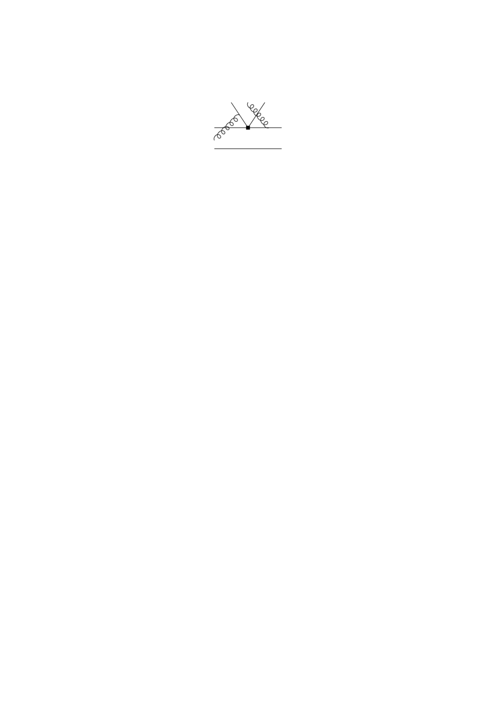
Let us study in more detail how the power suppression arises for the simplest non-trivial example, where the pion is composed of a quark, an antiquark, and an additional gluon. The contribution of this 3-particle Fock state to the $B\to D\pi$ decay amplitude is shown in Fig. 10. It is convenient to use the Fock–Schwinger gauge, which allows us to express the gluon field $A_{\lambda}$ in terms of the field-strength tensor $G_{\rho\lambda}$ via

$$A_{\lambda}(x)=\int^{1}_{0}\!dv\,vx^{\rho}\,G_{\rho\lambda}(vx)\,.$$ (48)

Up to twist-4 level, there are three quark–antiquark–gluon matrix elements that could potentially contribute to the diagrams shown in Fig. 10. Due to the $V-A$ structure of the weak-interaction vertex, the only relevant three-particle light-cone wave function has twist-4 and is given by $\!{}^{{\bf?},{\bf?}}$

$$\langle\pi(q)|\bar{d}(0)\gamma_{\mu}\gamma_{5}\,g_{s}G_{\alpha\beta}(vx)\,u(0)|0\rangle$$ (49)

$$= f_{\pi}(q_{\beta}g_{\alpha\mu}-q_{\alpha}g_{\beta\mu})\int{\cal D}u\,\phi_{\perp}(u_{i})\,e^{ivu_{3}q\cdot x}$$

$$+ f_{\pi}\,\frac{q_{\mu}}{q\cdot x}\,(q_{\alpha}x_{\beta}-q_{\beta}x_{\alpha})\int{\cal D}u\,\left(\phi_{\perp}(u_{i})+\phi_{\parallel}(u_{i})\right)e^{ivu_{3}q\cdot x}\,.$$

Here $\int{\cal D}u\equiv\int^{1}_{0}\!du_{1}\,du_{2}\,du_{3}\,\delta(1-u_{1}-u_{2}-u_{3})$, with $u_{1}$, $u_{2}$ and $u_{3}$ the fractions of the pion momentum carried by the quark, antiquark and gluon, respectively. Evaluating the diagrams in Fig. 10, and neglecting the charm-quark mass for simplicity, we find

$$\langle D^{+}\pi^{-}|O_{8}|\bar{B}_{d}\rangle_{q\bar{q}g}=if_{\pi}\,\langle D^{+}|\bar{c}\!\not\!q(1-\gamma_{5})b|\bar{B}_{d}\rangle\int{\cal D}u\,\frac{2\phi_{\parallel}(u_{i})}{u_{3}\,m^{2}_{b}}\,.$$ (50)

Since $\phi_{\parallel}\sim\Lambda^{2}_{\rm QCD}$, the suppression by two powers of $\Lambda_{\rm QCD}/m_{b}$ compared to the leading-order matrix element is obvious. Note that due to G-parity $\phi_{\parallel}$ is antisymmetric in $u_{1}\leftrightarrow u_{2}$ for a pion, so that (50) vanishes in this case.

Additional soft partons

A more precarious situation may arise when the additional Fock components carry only a small fraction of the meson momentum, contrary to the assumption made above. It is usually argued $\!{}^{{\bf?},{\bf?}}$ that these configurations are suppressed, because they occupy only a small fraction of the available phase space (since $\int du_{i}\sim\Lambda_{\rm QCD}/m_{b}$ when the parton that carries momentum fraction $u_{i}$ is soft). This argument does not apply when the process involves heavy mesons. Consider, for example, the diagram shown in Fig. 11 (a) for the decay $B\to D\pi$. Its contribution involves the overlap of the $B$-meson wave function involving additional soft gluons with the wave function of the $D$ meson, also containing soft gluons. There is no reason to suppose that this overlap is suppressed relative to the soft overlap of the valence-quark wave functions. It represents (part of) the overlap of the “soft cloud” around the $b$ quark with (part of) the “soft cloud” around the $c$ quark after the weak decay. The partonic decomposition of this cloud is unrestricted up to global quantum numbers. (In the case where the $B$ meson decays into two light mesons, there is a form-factor suppression $\sim(\Lambda_{\rm QCD}/m_{b})^{3/2}$ for the overlap of the valence-quark wave functions, but once this price is paid there is again no reason for further suppression of additional soft gluons in the overlap of the $B$-meson wave function and the wave function of the recoiling meson.)

Figure 11: (a) Soft overlap contribution which is part of the $B\to D$ form factor. (b) Soft overlap with the pion which would violate factorization, if it were unsuppressed.

The previous paragraph essentially repeated our earlier argument against the hard-scattering approach, and in favour of using the $B\to D$ form factor as an input to the factorization formula. However, given the presence of additional soft partons in the $B\to D$ transition, we must now argue that it is unlikely that the emitted pion drags with it one of these soft partons, for instance a soft gluon that goes into the pion wave function, as shown in Fig. 11 (b). Notice that if the $(q\bar{q})$ pair is produced in a colour-octet state, at least one gluon (or a further $(q\bar{q})$ pair) must be pulled into the emitted meson if the decay is to result in a two-body final state. What suppresses the process shown in Fig. 11 (b) relative to the one in Fig. 11 (a) even if the emitted $(q\bar{q})$ pair is in a colour-octet state?

It is once more colour transparency that saves us. The dominant configuration has both quarks carry a large fraction of the pion momentum, and only the gluon might be soft. In this situation we can apply a non-local “operator product expansion” to determine the coupling of the soft gluon to the small $(q\bar{q})$ pair $\!{}^{{\bf?}}$. The gluon endpoint behaviour of the $q\bar{q}g$ wave function is then determined by the sum of the two diagrams shown on the right-hand side in Fig. 12. The leading term (for small gluon momentum) cancels in the sum of the two diagrams, because the meson (represented by the black bar) is a colour singlet. This cancellation, which is exactly the same cancellation needed to demonstrate that “non-factorizable” vertex corrections are dominated by hard gluons, provides one factor of $\Lambda_{\rm QCD}/m_{b}$ needed to show that Fig. 11 (b) is power suppressed relative to Fig. 11 (a).

Figure 12: Quark–antiquark–gluon distribution amplitude in the gluon endpoint region.

In summary, we have (qualitatively) covered all possibilities for non-valence contributions to the decay amplitude and find that they are all power suppressed in the heavy-quark limit.

6 Limitations of the factorization approach

The factorization formula (2.2) holds in the heavy-quark limit $m_{b}\to\infty$. Corrections to the asymptotic limit are power-suppressed in the ratio $\Lambda_{\rm QCD}/m_{b}$ and, generally speaking, do not assume a factorized form. Since $m_{b}$ is fixed to about 5 GeV in the real world, one may worry about the magnitude of power corrections to hadronic $B$-decay amplitudes. Naive dimensional analysis would suggest that these corrections should be of order 10% or so. We now discuss several reasons why some power corrections could turn out to be numerically larger than suggested by the parametric suppression factor $\Lambda_{\rm QCD}/m_{b}$. Most of these “dangerous” corrections occur in more complicated, rare hadronic $B$ decays into two light mesons, but are absent in decays such as $B\to D\pi$.

6.1 Several small parameters

Large non-factorizable power corrections may arise if the leading-power, factorizable term is somehow suppressed. There are several possibilities for such a suppression, given a variety of small parameters that may enter into the non-leptonic decay amplitudes.

• The hard, “non-factorizable” effects computed using the factorization formula occur at order $\alpha_{s}$. Some other interesting effects such as final-state interactions appear first at this order. For instance, strong-interaction phases due to hard interactions are of order $\alpha_{s}$, while soft rescattering phases are of order $\Lambda_{\rm QCD}/m_{b}$. Since for realistic $B$ mesons $\alpha_{s}$ is not particularly large compared to $\Lambda_{\rm QCD}/m_{b}$, we should not expect that these phases can be calculated with great precision. In practice, however, it is probably more important to know that the strong-interaction phases are parametrically suppressed in the heavy-quark limit and thus should be small. (This does not apply if the real part of the decay amplitudes is suppressed for some reason; see below.)

• If the leading, lowest-order (in $\alpha_{s}$) contribution to the decay amplitude is colour suppressed, as occurs for the class-II decay $\bar{B}_{d}\to\pi^{0}\pi^{0}$, then perturbative and power corrections can be sizeable. In such a case even the hard strong-interaction phase of the amplitude can be large $\!{}^{{\bf?},{\bf?}}$. But at the same time soft contributions could be potentially important, so that in some cases only an order-of-magnitude estimate of the amplitude may be possible.

• The effective Hamiltonian (1) contains many Wilson coefficients $C_{i}$ that are small relative to $C_{1}\approx 1$. There are decays for which the entire leading-power contribution is suppressed by small Wilson coefficients, but some power-suppressed effects are not. An example of this type is $B^{-}\to K^{-}K^{0}$. This decay proceeds through a penguin operator $b\to ds\bar{s}$ at leading power. But the annihilation contribution, which is power suppressed, can occur through the current–current operator with large Wilson coefficient $C_{1}$. Our approach does not apply to such (presumably) annihilation-dominated decays, unless a systematic treatment of annihilation amplitudes can be found.

• Some amplitudes may be suppressed by a combination of small CKM matrix elements. For example, $B\to\pi K$ decays receive large penguin contributions despite their small Wilson coefficients, because the so-called tree amplitude is CKM suppressed. This is not a problem for factorization, since it applies to the penguin and the tree amplitudes. We are not aware of any case (for ordinary $B$ mesons) in which a purely power-suppressed term is CKM enhanced and which would therefore dominate the decay amplitude. (But this situation could occur for $B^{-}_{c}\to\bar{D}^{0}K^{-}$, where the QCD dynamics is similar if we consider the charm quark as a light quark.)

6.2 Power corrections enhanced by small quark masses

There is another enhancement of power-suppressed effects for some decays into two light mesons, connected with the curious numerical fact that

$$2\mu_{\pi}\equiv\frac{2m_{\pi}^{2}}{m_{u}+m_{d}}=-\frac{4\langle\bar{q}q\rangle}{f_{\pi}^{2}}\approx 3\,\mbox{GeV}$$ (51)

is much larger than its naive scaling estimate $\Lambda_{\rm QCD}$. (Here $\langle\bar{q}q\rangle=\langle 0|\bar{u}u|0\rangle=\langle 0|\bar{d}d|0\rangle$ is the quark condensate.) Consider the contribution of the penguin operator $O_{6}=(\bar{d}_{i}b_{j})_{V-A}(\bar{u}_{j}u_{i})_{V+A}$ to the $\bar{B}_{d}\to\pi^{+}\pi^{-}$ decay amplitude. The leading-order graph of Fig. 3 results in the expression

$$\langle\pi^{+}\pi^{-}|(\bar{d}_{i}b_{j})_{V-A}(\bar{u}_{j}u_{i})_{V+A}|\bar{B}_{d}\rangle=im_{B}^{2}\,F_{+}^{B\to\pi}(0)\,f_{\pi}\,\times\frac{2\mu_{\pi}}{m_{b}}\,,$$ (52)

which is formally a $\Lambda_{\rm QCD}/m_{b}$ power correction compared to the corresponding matrix element of a product of two left-handed currents, but numerically large due to (51). We would not have to worry about such terms if they could all be identified and the factorization formula (2.2) applied to them, since in this case higher-order perturbative corrections would not contain non-factorizing infrared logarithms. However, this is not the case.

After including radiative corrections, the matrix element on the left-hand side of (52) is expressed as a non-trivial convolution with pion light-cone distribution amplitudes. The terms involving $\mu_{\pi}$ can be related to two-particle twist-3 (rather than leading twist-2) distribution amplitudes, conventionally called $\Phi_{p}(u)$ and $\Phi_{\sigma}(u)$. We find that the radiative corrections to the matrix element in (52) do indeed factorize. However, at the same order there appear twist-3 corrections to the hard spectator interaction shown in Fig. 7, and these contributions contain an endpoint divergence (related to the fact that the distribution amplitudes $\Phi_{p}(u)$ and $\Phi^{\prime}_{\sigma}(u)$ do not vanish at the endpoints). In other words, the twist-3 “corrections” to the hard spectator term in the second factorization formula in (2.2) relative to the “leading” twist-2 contributions are of the form $\alpha_{s}\times\,$logarithmic divergence, which we interpret as being of order 1. The non-factorizing character of the “chirally-enhanced” power corrections can introduce a substantial uncertainty in some decay modes $\!{}^{{\bf?}}$. As in the related situation for the pion form factor $\!{}^{{\bf?}}$, one may argue that the endpoint divergence is suppressed by a Sudakov form factor. However, it is likely that when $m_{b}$ is not large enough to suppress these chirally-enhanced terms, then it is also not large enough to make Sudakov suppression effective.

We stress that the chirally-enhanced terms do not appear in decays into a heavy and a light meson such as $B\to D\pi$, because these decays have no penguin contribution and no contribution from the hard spectator interaction. Hence, the twist-3 light-cone distribution amplitudes responsible for chirally-enhanced power corrections do not enter in the evaluation of the decay amplitudes.

6.3 Non-leptonic decays when $M_{2}$ is not light

The analysis of non-leptonic decay amplitudes in Sect. 3.3 referred to decays where the emission particle $M_{2}$ is a light meson. We now briefly discuss the case where $M_{2}$ is heavy.

Suppose that $M_{2}$ is a $D$ meson, whereas the meson that picks up the spectator quark can be heavy or light. Examples of this type are the decays $\bar{B}_{d}\to\pi^{0}D^{0}$ and $\bar{B}_{d}\to D^{+}D^{-}$. It is intuitively clear that factorization must be problematic in these cases, because the heavy $D$ meson has a large overlap with the $\bar{B}\pi$ or $\bar{B}D$ systems, which are dominated by soft processes. In more detail, we consider the coupling of a gluon to the two quarks that form the emitted $D$ meson, i.e. the pairs of diagrams in Fig. 5 (a+b), (c+d) and Fig. 7. Denoting the gluon momentum by $k$, the quark momenta by $l_{q}$ and $l_{\bar{q}}$, and the $D$-meson momentum by $q$, we find that the gluon couples to the “current”

$$J_{\lambda}=\frac{\gamma_{\lambda}(\not\!l_{q}+\not\!k+m_{c})\Gamma}{2l_{q}\cdot k+k^{2}}-\frac{\Gamma(\not\!l_{\bar{q}}+\not\!k)\gamma_{\lambda}}{2l_{\bar{q}}\cdot k+k^{2}}\,,$$ (53)

where $\Gamma$ is part of the weak decay vertex. When $k$ is soft (all components of order $\Lambda_{\rm QCD}$), each of the two terms scales as $1/\Lambda_{\rm QCD}$. Taking into account the complete amplitude as done explicitly in Sect. 4.2, we can see that the decoupling of soft gluons requires that the two terms in (53) cancel, leaving a remainder of order $1/m_{b}$. This cancellation does indeed occur when $M_{2}$ is a light meson, since in this case $l_{q}$ and $l_{\bar{q}}$ are dominated by their longitudinal components. When $M_{2}$ is heavy, the momenta $l_{q}$ and $l_{\bar{q}}$ are asymmetric, with all components of the light antiquark momentum $l_{\bar{q}}$ of order $\Lambda_{\rm QCD}$ in the $B$- or $D$-meson rest frames, while the zero-component of $l_{q}$ is of order $m_{b}$. Hence the current can be approximated by

$$J_{\lambda}\approx\frac{\delta_{\lambda 0}\Gamma}{k_{0}}-\frac{\Gamma(\not\!l_{\bar{q}}+\not\!k)\gamma_{\lambda}}{2l_{\bar{q}}\cdot k+k^{2}}\sim\frac{1}{\Lambda_{\rm QCD}}\,,$$ (54)

and the soft cancellation does not occur. (The on-shell condition for the charm quark has been used to arrive at this equation.)

It follows that the emitted $D$ meson does not factorize from the rest of the process, and that a factorization formula analogous to (2.2) does not apply to decays such as $\bar{B}_{d}\to\pi^{0}D^{0}$ and $\bar{B}_{d}\to D^{+}D^{-}$. An important implication of this statement is that one should also not expect naive factorization to work in these cases. In other words, we expect that “non-factorizable” corrections modify the factorized decay amplitudes by terms of order 1.

6.4 Difficulties with charm

There are decay modes, such as $B^{-}\to D^{0}\pi^{-}$, in which the spectator quark can go to either of the two final-state mesons. The factorization formula (2.2) applies to the contribution that arises when the spectator quark goes to the $D$ meson, but not when the spectator quark goes to the pion. However, even in the latter case we may use naive factorization to estimate the power behaviour of the decay amplitude. Adapting (13) to the decay $B^{-}\to D^{0}\pi^{-}$, we find that the non-factorizing (class-II) amplitude is suppressed compared to the factorizing (class-I) amplitude by

$$\frac{{\cal A}(B^{-}\to D^{0}\pi^{-})_{\rm class\mbox{-}II}}{{\cal A}(B^{-}\to D^{0}\pi^{-})_{\rm class\mbox{-}I}}\sim\frac{F^{B\to\pi}(m_{D}^{2})\,f_{D}}{F^{B\to D}(m_{\pi}^{2})\,f_{\pi}}\sim\left(\frac{\Lambda_{\rm QCD}}{m_{b}}\right)^{2}.$$ (55)

Here we use that $F^{B\to\pi}(q^{2})\sim(\Lambda_{\rm QCD}/m_{b})^{3/2}$ even for $q^{2}\sim m_{b}^{2}$, as long as $q_{max}^{2}-q^{2}$ is also of order $m_{b}^{2}$. (It follows from our definition of heavy final-state mesons that these conditions are fulfilled.) As a consequence, strictly speaking factorization does hold for $B^{-}\to D^{0}\pi^{-}$ decays in the sense that the class-II contribution is power suppressed with respect to the class-I contribution.

Unfortunately, the scaling behaviour for real $B$ and $D$ mesons is far from the estimate (55) valid in the heavy-quark limit. Based on the dominance of the class-I amplitude we would expect that

$$R=\frac{\mbox{Br}(B^{-}\to D^{0}\pi^{-})}{\mbox{Br}(\bar{B}_{d}\to D^{+}\pi^{-})}\approx 1$$ (56)

in the heavy-quark limit. This contradicts existing data which yield $R=1.89\pm 0.35$, despite the additional colour suppression of the class-II amplitude. One reason for the failure of power counting lies in the departure of the decay constants and form factors from naive power counting. The following compares the power counting to the actual numbers (square brackets):

$$\frac{f_{D}}{f_{\pi}}\sim\left(\frac{\Lambda_{\rm QCD}}{m_{c}}\right)^{1/2}\,\,[\approx 1.5]\,,\qquad\frac{F_{+}^{B\to\pi}(m_{D}^{2})}{F_{+}^{B\to D}(m_{\pi}^{2})}\sim\left(\frac{\Lambda_{\rm QCD}}{m_{b}}\right)^{3/2}\,\,[\approx 0.5]\,.$$ (57)

However, it is unclear whether the failure of power counting can be attributed to the form factors and decay constants alone.

Note that for the purposes of power counting we treated the charm quark as heavy, taking the heavy-quark limit for fixed $m_{c}/m_{b}$. This simplified the discussion, since we did not have to introduce $m_{c}$ as a separate scale. However, in reality charm is somewhat intermediate between a heavy and a light quark, since $m_{c}$ is not particularly large compared to $\Lambda_{\rm QCD}$. In this context it is worth noting that the first hard-scattering kernel in (2.2) cannot have $\Lambda_{\rm QCD}/m_{c}$ corrections, since there is a smooth transition to the case of two light mesons. The situation is different with the hard spectator interaction term, which we argued to be power suppressed for decays into a $D$ meson and a light meson. We shall come back to this in Sect. 7.5, where we estimate the magnitude of this term for the $D\pi$ final state, relaxing the assumption that the $D$ meson is heavy.

7 Phenomenology of $B\to D^{(*)}L$ decays

The matrix elements we have computed in Sect. 4.3 provide the theoretical basis for a model-independent calculation of the class-I non-leptonic decay amplitudes for decays of the type $B\to D^{(*)}L$, where $L$ is a light meson, to leading power in $\Lambda_{\rm QCD}/m_{b}$ and at next-to-leading order in renormalization-group improved perturbation theory. In this section we discuss phenomenological applications of this formalism and confront our numerical results with experiment. We also provide some numerical estimates of power-suppressed corrections to the factorization formula.

7.1 Non-leptonic decay amplitudes

The results for the class-I decay amplitudes for $B\to D^{(*)}L$ are obtained by evaluating the (factorized) hadronic matrix elements of the transition operator ${\cal T}$ defined in (40). They are written in terms of products of CKM matrix elements, light-meson decay constants, $B\to D^{(*)}$ transition form factors, and the QCD parameters $a_{1}(D^{(*)}L)$. The decay constants can be determined experimentally using data on the weak leptonic decays $P^{-}\to l^{-}\bar{\nu}_{l}(\gamma)$, hadronic $\tau^{-}\to M^{-}\nu_{\tau}$ decays, and the electromagnetic decays $V^{0}\to e^{+}e^{-}$. Following $\!{}^{{\bf?}}$, we use $f_{\pi}=131$ MeV, $f_{K}=160$ MeV, $f_{\rho}=210$ MeV, $f_{K^{*}}=214$ MeV, and $f_{a_{1}}=229$ MeV. (Here $a_{1}$ is the pseudovector meson with mass $m_{a_{1}}\simeq 1230$ MeV.)

The non-leptonic $\bar{B}_{d}\to D^{(*)+}L^{-}$ decay amplitudes for $L=\pi$, $\rho$ can be expressed as

$${\cal A}(\bar{B}_{d}\to D^{+}\pi^{-}) = i\frac{G_{F}}{\sqrt{2}}\,V^{*}_{ud}V_{cb}\,a_{1}(D\pi)\,f_{\pi}\,F_{0}(m^{2}_{\pi})\,(m^{2}_{B}-m^{2}_{D})\,,$$

$${\cal A}(\bar{B}_{d}\to D^{*+}\pi^{-}) = -i\frac{G_{F}}{\sqrt{2}}\,V^{*}_{ud}V_{cb}\,a_{1}(D^{*}\pi)\,f_{\pi}A_{0}(m^{2}_{\pi})\,2m_{D^{*}}\,\varepsilon^{*}\!\cdot p\,,$$

$${\cal A}(\bar{B}_{d}\to D^{+}\rho^{-}) = -i\frac{G_{F}}{\sqrt{2}}\,V^{*}_{ud}V_{cb}\,a_{1}(D\rho)\,f_{\rho}\,F_{+}(m^{2}_{\rho})\,2m_{\rho}\,\eta^{*}\!\cdot p\,,$$ (58)

where $p$ ($p^{\prime}$) is the momentum of the $B$ (charm) meson, $\varepsilon$ and $\eta$ are polarization vectors, and the form factors $F_{0}$, $F_{+}$ and $A_{0}$ are defined in the usual way $\!{}^{{\bf?}}$. The decay mode $\bar{B}_{d}\to D^{*+}\rho^{-}$ has a richer structure than the decays with at least one pseudoscalar in the final state. The most general Lorentz-invariant decomposition of the corresponding decay amplitude can be written as

$${\cal A}(\bar{B}_{d}\to D^{*+}\rho^{-})=i\frac{G_{F}}{\sqrt{2}}\,V^{*}_{ud}V_{cb}\,\varepsilon^{*\mu}\eta^{*\nu}\bigg{(}S_{1}\,g_{\mu\nu}-S_{2}\,q_{\mu}p^{\prime}_{\nu}+iS_{3}\,\epsilon_{\mu\nu\alpha\beta}\,p^{\prime\alpha}q^{\beta}\bigg{)}\,,$$ (59)

where the quantities $S_{i}$ can be expressed in terms of semi-leptonic form factors. To leading power in $\Lambda_{\rm QCD}/m_{b}$, we obtain

$$S_{1} = a_{1}(D^{*}\rho)\,m_{\rho}f_{\rho}\,(m_{B}+m_{D^{*}})A_{1}(m_{\rho}^{2})\,,$$

$$S_{2} = a_{1}(D^{*}\rho)\,m_{\rho}f_{\rho}\,\frac{2A_{2}(m_{\rho}^{2})}{m_{B}+m_{D^{*}}}\,.$$ (60)

The contribution proportional to $S_{3}$ in (59) is associated with transversely polarized $\rho$ mesons and thus leads to power-suppressed effects, which we do not consider here.

The various $B\to D^{(*)}$ form factors entering the expressions for the decay amplitudes can be determined by combining experimental data on semi-leptonic decays with theoretical relations derived using heavy-quark effective theory $\!{}^{{\bf?},{\bf?}}$. Since we work to leading order in $\Lambda_{\rm QCD}/m_{b}$, it is consistent to set the light meson masses to zero and evaluate these form factors at $q^{2}=0$. In this case the kinematic relations

$$F_{0}(0)=F_{+}(0)\,,\qquad(m_{B}+m_{D^{*}})A_{1}(0)-(m_{B}-m_{D^{*}})A_{2}(0)=2m_{D^{*}}A_{0}(0)$$ (61)

allow us to express the two $\bar{B}_{d}\to D^{+}L^{-}$ rates in terms of $F_{+}(0)$, and the two $\bar{B}_{d}\to D^{*+}L^{-}$ rates in terms of $A_{0}(0)$. Heavy-quark symmetry implies that these two form factors are equal to within a few percent $\!{}^{{\bf?}}$. Below we adopt the common value $F_{+}(0)=A_{0}(0)=0.6$. All our predictions for decay rates will be proportional to the square of this number.

7.2 Meson distribution amplitudes and predictions for $a_{1}$

Let us now discuss in more detail the ingredients required for the numerical analysis of the coefficients $a_{1}(D^{(*)}L)$. The Wilson coefficients $C_{i}$ in the effective weak Hamiltonian depend on the choice of the scale $\mu$ as well as on the value of the strong coupling $\alpha_{s}$, for which we take $\alpha_{s}(m_{Z})=0.118$ and two-loop evolution down to a scale $\mu\sim m_{b}$. To study the residual scale dependence of the results, which remains because the perturbation series are truncated at next-to-leading order, we vary $\mu$ between $m_{b}/2$ and $2m_{b}$. The hard-scattering kernels depend on the ratio of the heavy-quark masses, for which we take $z=m_{c}/m_{b}=0.30\pm 0.05$.

Table 1: Numerical values for the integrals $\int^{1}_{0}du\,F(u,z)\,\Phi_{L}(u)$ (upper portion) and $\int^{1}_{0}du\,F(u,-z)\,\Phi_{L}(u)$ (lower portion) obtained including the first two Gegenbauer moments.

$z$	Leading term	Coefficient of $\alpha_{1}^{L}$	Coefficient of $\alpha_{2}^{L}$
0.25	$-8.41-9.51i$	$5.92-12.19i$	$-1.33+0.36i$
0.30	$-8.79-9.09i$	$5.78-12.71i$	$-1.19+0.58i$
0.35	$-9.13-8.59i$	$5.60-13.21i$	$-1.00+0.73i$
0.25	$-8.45-6.56i$	$6.72-10.73i$	$-0.38+0.93i$
0.30	$-8.37-5.99i$	$6.83-11.49i$	$-0.21+0.85i$
0.35	$-8.24-5.44i$	$6.81-12.29i$	$-0.08+0.75i$

Hadronic uncertainties enter the analysis also through the parameterizations used for the meson light-cone distribution amplitudes. It is convenient and conventional to expand the distribution amplitudes in Gegenbauer polynomials as

$$\Phi_{L}(u)=6u(1-u)\left[1+\sum_{n=1}^{\infty}\alpha_{n}^{L}(\mu)\,C_{n}^{(3/2)}(2u-1)\right]\,,$$ (62)

where $C_{1}^{(3/2)}(x)=3x$, $C_{2}^{(3/2)}(x)=\frac{3}{2}(5x^{2}-1)$, etc. The Gegenbauer moments $\alpha_{n}^{L}(\mu)$ are multiplicatively renormalized. The scale dependence of these quantities would, however, enter the results for the coefficients only at order $\alpha_{s}^{2}$, which is beyond the accuracy of our calculation. We assume that the leading-twist distribution amplitudes are close to their asymptotic form and thus truncate the expansion at $n=2$. However, it would be straightforward to account for higher-order terms if desired. For the asymptotic form of the distribution amplitude, $\Phi_{L}(u)=6u(1-u)$, the integral in (4.3) yields

$$\int^{1}_{0}du\,F(u,z)\,\Phi_{L}(u)=3\ln z^{2}-7$$

$$\quad\mbox{}+\Bigg{[}\frac{6z(1-2z)}{(1-z)^{2}(1+z)^{3}}\left(\frac{\pi^{2}}{6}-\mbox{Li}_{2}(z^{2})\right)-\frac{3(2-3z+2z^{2}+z^{3})}{(1-z)(1+z)^{2}}\ln(1-z^{2})$$

$$\qquad\hskip 8.5359pt\mbox{}+\frac{4-17z+20z^{2}+5z^{3}}{2(1-z)(1+z)^{2}}+\{z\to 1/z\}\Bigg{]}\,,$$ (63)

and the corresponding result with the function $F(u,-z)$ is obtained by replacing $z\to-z$. More generally, a numerical integration with a distribution amplitude expanded in Gegenbauer polynomials yields the results collected in Table 1. We observe that the first two Gegenbauer polynomials in the expansion of the light-cone distribution amplitudes give contributions of similar magnitude, whereas the second moment gives rise to much smaller effects. This tendency persists in higher orders. For our numerical discussion it is a safe approximation to truncate the expansion after the first non-trivial moment. The dependence of the results on the value of the quark mass ratio $z=m_{c}/m_{b}$ is mild and can be neglected for all practical purposes. We also note that the difference of the convolutions with the kernels for a pseudoscalar $D$ and vector $D^{*}$ meson are numerically very small. This observation is, however, specific to the case of $B\to D^{(*)}L$ decays and should not be generalized to other decays.

Table 2: The QCD coefficients $a_{1}(D^{(*)}L)$ at next-to-leading order for three different values of the renormalization scale $\mu$. The leading-order values are shown for comparison.

	$\mu=m_{b}/2$	$\mu=m_{b}$	$\mu=2m_{b}$
$a_{1}(DL)$	$1.074+0.037i$	$1.055+0.020i$	$1.038+0.011i$
	$-(0.024-0.052i)\,\alpha_{1}^{L}$	$-(0.013-0.028i)\,\alpha_{1}^{L}$	$-(0.007-0.015i)\,\alpha_{1}^{L}$
$a_{1}(D^{*}L)$	$1.072+0.024i$	$1.054+0.013i$	$1.037+0.007i$
	$-(0.028-0.047i)\,\alpha_{1}^{L}$	$-(0.015-0.025i)\,\alpha_{1}^{L}$	$-(0.008-0.014i)\,\alpha_{1}^{L}$
$a^{\rm LO}_{1}$	$1.049$	$1.025$	$1.011$

Next we evaluate the complete results for the parameters $a_{1}$ at next-to-leading order, and to leading power in $\Lambda_{\rm QCD}/m_{b}$. We set $z=m_{c}/m_{b}=0.3$. Varying $z$ between 0.25 and 0.35 would change the results by less than 0.5%. The results are shown in Table 2. The contributions proportional to the second Gegenbauer moment $\alpha_{2}^{L}$ have coefficients of order 0.2% or less and can safely be neglected. The contributions associated with $\alpha_{1}^{L}$ are present only for the strange mesons $K$ and $K^{*}$, but not for $\pi$ and $\rho$. Moreover, the imaginary parts of the coefficients contribute to their modulus only at order $\alpha_{s}^{2}$, which is beyond the accuracy of our analysis. To summarize, we thus obtain

$$|a_{1}(DL)| = 1.055_{-0.017}^{+0.019}-(0.013_{-0.006}^{+0.011})\alpha_{1}^{L}\,,$$

$$|a_{1}(D^{*}L)| = 1.054_{-0.017}^{+0.018}-(0.015_{-0.007}^{+0.013})\alpha_{1}^{L}\,,$$ (64)

where the quoted errors reflect the perturbative uncertainty due to the scale ambiguity (and the negligible dependence on the value of the ratio of quark masses and higher Gegenbauer moments), but not the effects of power-suppressed corrections. These will be estimated later. It is evident that within theoretical uncertainties there is no significant difference between the two $a_{1}$ parameters, and there is only a very small sensitivity to the differences between strange and non-strange mesons (assuming that $|\alpha_{1}^{K^{(*)}}|<1$). In our numerical analysis below we thus take $|a_{1}|=1.05$ for all decay modes.

7.3 Tests of factorization

The main lesson from the previous discussion is that corrections to naive factorization in the class-I decays $\bar{B}_{d}\to D^{(*)+}L^{-}$ are very small. The reason is that these effects are governed by a small Wilson coefficient and, moreover, are colour suppressed by a factor $1/N_{c}^{2}$. For these decays, the most important implications of the QCD factorization formula are to restore the renormalization-group invariance of the theoretical predictions, and to provide a theoretical justification for why naive factorization works so well. On the other hand, given the theoretical uncertainties arising, e.g., from unknown power-suppressed corrections, there is little hope to confront the extremely small predictions for non-universal (process-dependent) “non-factorizable” corrections with experimental data. Rather, what we may do is ask whether data supports the prediction of a quasi-universal parameter $|a_{1}|\simeq 1.05$ in these decays. If this is indeed the case, it would support the usefulness of the heavy-quark limit in analyzing non-leptonic decay amplitudes. If, on the other hand, we were to find large non-universal effects, this would point towards the existence of sizeable power corrections to our predictions. We will see that within present experimental errors the data are in good agreement with our prediction of a quasi universal $a_{1}$ parameter. However, a reduction of the experimental uncertainties to the percent level would be very desirable for obtaining a more conclusive picture.

We start by considering ratios of non-leptonic decay rates that are related to each other by the replacement of a pseudoscalar meson by a vector meson. In the comparison of $B\to D\pi$ and $B\to D^{*}\pi$ decays one is sensitive to the difference of the values of the two $a_{1}$ parameters in (7.2) evaluated for $\alpha_{1}^{L}=0$. This difference is at most few times $10^{-3}$. Likewise, in the comparison of $B\to D\pi$ and $B\to D\rho$ decays one is sensitive to the difference in the light-cone distribution amplitudes of the pion and the $\rho$ meson, which start at the second Gegenbauer moment $\alpha_{2}^{L}$. These effects are suppressed even more strongly. From the explicit expressions for the decay amplitudes in (7.1) it follows that

$$\frac{\Gamma(\bar{B}_{d}\to D^{+}\pi^{-})}{\Gamma(\bar{B}_{d}\to D^{*+}\pi^{-})} = \frac{(m_{B}^{2}-m_{D}^{2})^{2}|\vec{q}\,|_{D\pi}}{4m_{B}^{2}|\vec{q}\,|_{D^{*}\pi}^{3}}\left(\frac{F_{0}(m_{\pi}^{2})}{A_{0}(m_{\pi}^{2})}\right)^{2}\left|\frac{a_{1}(D\pi)}{a_{1}(D^{*}\pi)}\right|^{2},$$

$$\frac{\Gamma(\bar{B}_{d}\to D^{+}\rho^{-})}{\Gamma(\bar{B}_{d}\to D^{+}\pi^{-})} = \frac{4m_{B}^{2}|\vec{q}\,|_{D\rho}^{3}}{(m_{B}^{2}-m_{D}^{2})^{2}|\vec{q}\,|_{D\pi}}\,\frac{f_{\rho}^{2}}{f_{\pi}^{2}}\,\left(\frac{F_{+}(m_{\rho}^{2})}{F_{0}(m_{\pi}^{2})}\right)^{2}\left|\frac{a_{1}(D\rho)}{a_{1}(D\pi)}\right|^{2}.~{}~{}$$ (65)

Using the experimental values for the branching ratios reported by the CLEO Collaboration $\!{}^{{\bf?}}$ we find (taking into account a correlation between some systematic errors in the second case)

$$\left|\frac{a_{1}(D\pi)}{a_{1}(D^{*}\pi)}\right|\,\frac{F_{0}(m_{\pi}^{2})}{A_{0}(m_{\pi}^{2})} = 1.00\pm 0.11\,,$$

$$\left|\frac{a_{1}(D\rho)}{a_{1}(D\pi)}\right|\,\frac{F_{+}(m_{\rho}^{2})}{F_{0}(m_{\pi}^{2})} = 1.16\pm 0.11\,.$$ (66)

Within errors, there is no evidence for any deviations from naive factorization.

Our next-to-leading order results for the quantities $a_{1}(D^{(*)}L)$ allow us to make theoretical predictions which are not restricted to ratios of hadronic decay rates. A particularly clean test of these predictions, which is essentially free of hadronic uncertainties, is obtained by relating the $\bar{B}_{d}\to D^{(*)+}L^{-}$ decay rates to the differential semi-leptonic $\bar{B}_{d}\to D^{(*)+}\,l^{-}\nu$ decay rate evaluated at $q^{2}=m_{L}^{2}$. In this way the parameters $|a_{1}|$ can be measured directly $\!{}^{{\bf?}}$. One obtains

$$R_{L}^{(*)}=\frac{\Gamma(\bar{B}_{d}\to D^{(*)+}L^{-})}{d\Gamma(\bar{B}_{d}\to D^{(*)+}l^{-}\bar{\nu})/dq^{2}\big{|}_{q^{2}=m^{2}_{L}}}=6\pi^{2}|V_{ud}|^{2}f^{2}_{L}\,|a_{1}(D^{(*)}L)|^{2}\,X^{(*)}_{L}\,,$$ (67)

where $X_{\rho}=X_{\rho}^{*}=1$ for a vector meson (because the production of the lepton pair via a $V-A$ current in semi-leptonic decays is kinematically equivalent to that of a vector meson with momentum $q$), whereas $X_{\pi}$ and $X_{\pi}^{*}$ deviate from 1 only by (calculable) terms of order $m_{\pi}^{2}/m_{B}^{2}$, which numerically are below the 1% level $\!{}^{{\bf?}}$. We emphasize that with our results for $a_{1}$ given in (4.3) the above relation becomes a prediction based on first principles of QCD. This is to be contrasted with the usual interpretation of this formula, where $a_{1}$ plays the role of a phenomenological parameter that is fitted from data.

The most accurate tests of factorization employ the class-I processes $\bar{B}_{d}\to D^{*+}L^{-}$, because the differential semi-leptonic decay rate in $B\to D^{*}$ transitions has been measured as a function of $q^{2}$ with good accuracy. The results of such an analysis, performed using CLEO data, have been reported in $\!{}^{{\bf?}}$. One finds

$$R_{\pi}^{*}=(1.13\pm 0.15)\,\mbox{GeV}^{2}\quad \Rightarrow \quad|a_{1}(D^{*}\pi)|=1.08\pm 0.07\,,$$

$$R_{\rho}^{*}=(2.94\pm 0.54)\,\mbox{GeV}^{2}\quad \Rightarrow \quad|a_{1}(D^{*}\rho)|=1.09\pm 0.10\,,$$

$$R_{a_{1}}^{*}=(3.45\pm 0.69)\,\mbox{GeV}^{2}\quad \Rightarrow \quad|a_{1}(D^{*}a_{1})|=1.08\pm 0.11\,.$$ (68)

This is consistent with our theoretical result in (4.3). In particular, the data show no evidence for large power corrections to our predictions obtained at leading order in $\Lambda_{\rm QCD}/m_{b}$. However, a further improvement in the experimental accuracy would be desirable in order to become sensitive to process-dependent, non-factorizable effects.

7.4 Predictions for class-I decay amplitudes

We now consider a larger set of class-I decays of the form $\bar{B}_{d}\to D^{(*)+}L^{-}$, all of which are governed by the transition operator (40). In Table 3 we compare the QCD factorization predictions with experimental data. As previously we work in the heavy-quark limit, i.e. our predictions are model independent up to corrections suppressed by at least one power of $\Lambda_{\rm QCD}/m_{b}$. The results show good agreement with experiment within errors, which are still rather large. (Note that we have not attempted to adjust the semi-leptonic form factors $F_{+}(0)$ and $A_{0}(0)$ so as to obtain a best fit to the data.)

Table 3: Model-independent predictions for the branching ratios (in units of $10^{-3}$) of class-I, non-leptonic $\bar{B}_{d}\to D^{(*)+}L^{-}$ decays in the heavy-quark limit. All predictions are in units of $(|a_{1}|/1.05)^{2}$. The last two columns show the experimental results reported by the CLEO Collaboration $\!{}^{{\bf?}}$, and by the Particle Data Group $\!{}^{{\bf?}}$.

Decay mode	Theory (HQL)	CLEO data	PDG98
$\bar{B}_{d}\to D^{+}\pi^{-}$	3.27	$2.50\pm 0.40$	$3.0\pm 0.4$
$\bar{B}_{d}\to D^{+}K^{-}$	0.25	—	—
$\bar{B}_{d}\to D^{+}\rho^{-}$	7.64	$7.89\pm 1.39$	$7.9\pm 1.4$
$\bar{B}_{d}\to D^{+}K^{*-}$	0.39	—	—
$\bar{B}_{d}\to D^{+}a_{1}^{-}$	7.76	$8.34\pm 1.66$	$6.0\pm 3.3$
	$\times[F_{+}(0)/0.6]^{2}$
$\bar{B}_{d}\to D^{*+}\pi^{-}$	3.05	$2.34\pm 0.32$	$2.8\pm 0.2$
$\bar{B}_{d}\to D^{*+}K^{-}$	0.22	—	—
$\bar{B}_{d}\to D^{*+}\rho^{-}$	7.59	$7.34\pm 1.00$	$6.7\pm 3.3$
$\bar{B}_{d}\to D^{*+}K^{*-}$	0.40	—	—
$\bar{B}_{d}\to D^{*+}a_{1}^{-}$	8.53	$11.57\pm 2.02$	$13.0\pm 2.7$
	$\times[A_{0}(0)/0.6]^{2}$

We take the observation that the experimental data on class-I decays into heavy-light final states show good agreement with our predictions obtained in the heavy-quark limit as evidence that in these decays there are no unexpectedly large power corrections. We will now address the important question of the size of power corrections theoretically. To this end we provide rough estimates of two sources of power-suppressed effects: weak annihilation and spectator interactions. We stress that, at present, a complete account of power corrections to the heavy-quark limit cannot be performed in a systematic way, since these effects are not dominated by hard gluon exchange. In other words, factorization breaks down beyond leading power, and there are other sources of power corrections, such as contributions from higher Fock states, which we will not address here. We believe that the estimates presented below are nevertheless instructive.

To obtain an estimate of power corrections we adopt the following, heuristic procedure. We treat the charm quark as light compared to the large scale provided by the mass of the decaying $b$ quark ($m_{c}\ll m_{b}$, and $m_{c}$ fixed as $m_{b}\to\infty$) and use a light-cone projection similar to that of the pion also for the $D$ meson. In addition, we assume that $m_{c}$ is still large compared to $\Lambda_{\rm QCD}$. We implement this by using a highly asymmetric $D$-meson wave function, which is strongly peaked at a light-quark momentum fraction of order $\Lambda_{\rm QCD}/m_{D}$. This guarantees correct power counting for the heavy-light final states we are interested in. As discussed in Sect. 5.2, there are four annihilation diagrams with a single gluon exchange (see Fig. 8 (a)–(d)). The first two diagrams are “factorizable” and their contributions vanish because of current conservation in the limit $m_{c}\to 0$. For non-zero $m_{c}$ they therefore carry an additional suppression factor $m^{2}_{D}/m^{2}_{B}\approx 0.1$. Moreover, their contributions to the decay amplitude are suppressed by small Wilson coefficients. Diagrams (a) and (b) can therefore safely be neglected. From the non-factorizable diagrams (c) and (d) in Fig. 8, the one with the gluon attached to the $b$ quark turns out to be strongly suppressed numerically, giving a contribution of less than $1\%$ of the leading class-I amplitude. We are thus left with diagram (d), in which the gluon couples to the light quark in the $B$ meson. This mechanism gives the dominant annihilation contribution. (Note that by deforming the light spectator-quark line one can redraw this diagram in such a way that it can be interpreted as a final-state rescattering process.)

Adopting a common notation, we parameterize the annihilation contribution to the $\bar{B}_{d}\to D^{+}\pi^{-}$ decay amplitude in terms of a (power-suppressed) amplitude $A$ such that ${\cal A}(\bar{B}_{d}\to D^{+}\pi^{-})=T+A$, where $T$ is the “tree topology”, which contains the dominant factorizable contribution. A straightforward calculation using the approximations discussed above shows that the contribution of diagram (d) is (to leading order) independent of the momentum fraction $\xi$ of the light quark inside the $B$ meson:

$$A\simeq f_{\pi}f_{D}f_{B}\int du\,\frac{\Phi_{\pi}(u)}{u}\int dv\,\frac{\Phi_{D}(v)}{\bar{v}^{2}}\simeq 3f_{\pi}f_{D}f_{B}\,\int dv\,\frac{\Phi_{D}(v)}{\bar{v}^{2}}\,.$$ (69)

The $B$-meson wave function simply integrates to $f_{B}$, and the integral over the pion distribution amplitude can be performed using the asymptotic form of the wave function. We take $\Phi_{D}(v)$ in the form of (62) with the coefficients $\alpha^{D}_{1}=0.8$ and $\alpha^{D}_{2}=0.4$ ($\alpha^{D}_{i}=0$, $i>2$). With this ansatz $\Phi_{D}(v)$ is strongly peaked at $\bar{v}\sim\Lambda_{\rm QCD}/m_{D}$. The integral over $\Phi_{D}(v)$ in (69) is divergent at $v=1$, and we regulate it by introducing a cut-off such that $v\leq 1-\Lambda/m_{B}$ with $\Lambda\approx 0.3$ GeV. Then $\int dv\,\Phi_{D}(v)/\bar{v}^{2}\approx 34$. Evidently, the proper value of $\Lambda$ is largely unknown, and our estimate will be correspondingly uncertain. Nevertheless, this exercise will give us an idea of the magnitude of the effect. For the ratio of the annihilation amplitude to the leading, factorizable contribution we obtain

$$\frac{A}{T}\simeq\frac{2\pi\alpha_{s}}{3}\,\frac{C_{+}+C_{-}}{2C_{+}+C_{-}}\,\frac{f_{D}f_{B}}{F_{0}(0)\,m_{B}^{2}}\int dv\,\frac{\Phi_{D}(v)}{\bar{v}^{2}}\approx 0.04\,.$$ (70)

We have evaluated the Wilson coefficients at $\mu=m_{b}$ and used $f_{D}=0.2$ GeV, $f_{B}=0.18$ GeV, $F_{0}(0)=0.6$, and $\alpha_{s}=0.4$. This value of the strong coupling constant reflects that the typical virtuality of the gluon propagator in the annihilation graph is of order $\Lambda_{\rm QCD}m_{B}$. We conclude that the annihilation contribution is a correction of a few percent, which is what one would expect for a generic power correction to the heavy-quark limit. Taking into account that $f_{B}\sim\Lambda_{\rm QCD}(\Lambda_{\rm QCD}/m_{B})^{1/2}$, $F_{0}(0)\sim(\Lambda_{\rm QCD}/m_{B})^{3/2}$ and $f_{D}\sim\Lambda_{\rm QCD}$, we observe that in the heavy-quark limit the ratio $A/T$ indeed scales as $\Lambda_{\rm QCD}/m_{b}$, exhibiting the expected linear power suppression. (Recall that we consider the $D$ meson as a light meson for this heuristic analysis of power corrections.)

Using the same approach, we may also derive a numerical estimate for the non-factorizable spectator interaction in $\bar{B}_{d}\to D^{+}\pi^{-}$ decays, discussed in Sect. 5.1. We find

$$\frac{T_{\rm spec}}{T_{\rm lead}}\simeq\frac{2\pi\alpha_{s}}{3}\,\frac{C_{+}-C_{-}}{2C_{+}+C_{-}}\,\frac{f_{D}f_{B}}{F_{0}(0)\,m_{B}^{2}}\frac{m_{B}}{\lambda_{B}}\int dv\,\frac{\Phi_{D}(v)}{\bar{v}}\approx-0.03\,,$$ (71)

where the hadronic parameter $\lambda_{B}=O(\Lambda_{\rm QCD})$ is defined as $\int_{0}^{1}(d\xi/\xi)\,\Phi_{B}(\xi)\equiv m_{B}/\lambda_{B}$. For the numerical estimate we have assumed that $\lambda_{B}\approx 0.3$ GeV. With the same model for $\Phi_{D}(v)$ as above we have $\int dv\,\Phi_{D}(v)/\bar{v}\approx 6.6$, where the integral is now convergent. The result (71) exhibits again the expected power suppression in the heavy-quark limit, and the numerical size of the effect is at the few percent level.

We conclude from this discussion that the typical size of power corrections to the heavy-quark limit in class-I decays of $B$ mesons into heavy-light final states is at the level of 10% or less, and thus our prediction for the near universality of the parameters $a_{1}$ governing these decay modes appears robust.

7.5 Remarks on class-II and class-III decay amplitudes

In the class-I decays $\bar{B}_{d}\to D^{(*)+}L^{-}$, the flavour quantum numbers of the final-state mesons ensure that only the light meson $L$ can be produced by the $(\bar{d}u)$ current contained in the operators of the effective weak Hamiltonian in (15). The QCD factorization formula then predicts that the corresponding decay amplitudes are factorizable in the heavy-quark limit. The formula also predicts that other topologies, in which the heavy charm meson would be created by a $(\bar{c}u)$ current, are power suppressed. To study these topologies we now consider decays with a neutral charm meson in the final state. In the class-II decays $\bar{B}_{d}\to D^{(*)0}L^{0}$ the only possible topology is to have the charm meson as the emission particle, whereas for the class-III decays $B^{-}\to D^{(*)0}L^{-}$ both final-state mesons can be the emission particle. The factorization formula predicts that in the heavy-quark limit class-II decay amplitudes are power suppressed with respect to the corresponding class-I amplitudes, whereas class-III amplitudes should be equal to the corresponding class-I amplitudes up to power corrections.

It is convenient to introduce two common parameterizations of the decay amplitudes, one in terms of isospin amplitudes $A_{1/2}$ and $A_{3/2}$ referring to the isospin of the final-state particles, and one in terms of flavour topologies ($T$ for “tree topology”, $C$ for “colour suppressed tree topology”, and $A$ for “annihilation topology”). Taking the decays $B\to D\pi$ as an example, we have

$${\cal A}(\bar{B}_{d}\to D^{+}\pi^{-}) = \sqrt{\frac{1}{3}}A_{3/2}+\sqrt{\frac{2}{3}}A_{1/2}=T+A\,,$$

$$\sqrt{2}\,{\cal A}(\bar{B}_{d}\to D^{0}\pi^{0}) = \sqrt{\frac{4}{3}}A_{3/2}-\sqrt{\frac{2}{3}}A_{1/2}=C-A\,,$$

$${\cal A}(B^{-}\to D^{0}\pi^{-}) = \sqrt{3}A_{3/2}=T+C\,.$$ (72)

A similar decomposition holds for the other $B\to D^{(*)}L$ decay modes. Isospin symmetry of the strong interactions implies that the class-III amplitude is a linear combination of the class-I and class-II amplitudes. In other words, there are only two independent amplitudes, which can be taken to be $A_{1/2}$ and $A_{3/2}$, or $(T+A)$ and $(C-A)$. These amplitudes are complex due to strong-interaction phases from final-state interactions. Only the relative phase of the two independent amplitudes is an observable. We define $\delta$ to be the relative phase of $A_{1/2}$ and $A_{3/2}$, and $\delta_{TC}$ the relative phase of $(T+A)$ and $(C-A)$. The QCD factorization formula implies that

$$\frac{A_{1/2}}{\sqrt{2}\,A_{3/2}} = 1+O(\Lambda_{\rm QCD}/m_{b})\,,\qquad\delta=O(\Lambda_{\rm QCD}/m_{b})\,,$$

$$\frac{C-A}{T+A} = O(\Lambda_{\rm QCD}/m_{b})\,,\hskip 25.6073pt\delta_{TC}=O(1)\,.$$ (73)

In the remainder of this section, we will explore to what extent these predictions are supported by data.

Table 4: CLEO data $\!{}^{{\bf?},{\bf?}}$ on the branching ratios for the decays $B\to D^{(*)}L$ in units of $10^{-3}$. Upper limits are at 90% confidence level. See text for the definition of the quantities $\delta$ and ${\cal R}$.

	$B\to D\pi$	$B\to D\rho$	$B\to D^{*}\pi$	$B\to D^{*}\rho$
Class-I   ($D^{(*)+}L^{-}$)	$2.50\pm 0.40$	$7.89\pm 1.39$	$2.34\pm 0.32$	$7.34\pm 1.00$
Class-II   ($D^{(*)0}L^{0}$)	$<0.12$	$<0.39$	$<0.44$	$<0.56$
Class-III ($D^{(*)0}L^{-}$)	$4.73\pm 0.44$	$9.20\pm 1.11$	$3.92\pm 0.63$	$12.77\pm 1.94$
$\delta$	$<22^{\circ}$	$<30^{\circ}$	$<57^{\circ}$	$<31^{\circ}$
${\cal R}$	$1.34\pm 0.13$	$1.05\pm 0.12$	$1.26\pm 0.14$	$1.28\pm 0.13$

In Table 4 we show the experimental results for the various $B\to D^{(*)}L$ branching ratios reported by the CLEO Collaboration $\!{}^{{\bf?},{\bf?}}$. We first note that no evidence has been seen for any of the class-II decays, in accordance with our prediction that these decays are suppressed with respect to the class-I modes. Below we will investigate in more detail how this suppression is realized. The fourth line in the table shows upper limits on the strong-interaction phase difference $\delta$ between the two isospin amplitudes, which follow from the relation $\!{}^{{\bf?}}$

$$\sin^{2}\!\delta<\frac{9}{2}\,\frac{\tau(B^{-})}{\tau(B_{d})}\,\frac{\mbox{Br}(\bar{B}_{d}\to D^{0}\pi^{0})}{\mbox{Br}(B^{-}\to D^{0}\pi^{-})}\,.$$ (74)

The strongest bound arises in the decays $B\to D\pi$, where the strong-interaction phase is bound to be less than $22^{\circ}$. This confirms our prediction that the phase $\delta$ is suppressed in the heavy-quark limit.

Let us now study the suppression of the class-II amplitudes in more detail. We have already mentioned in Sect. 6.4 that the observed smallness of these amplitudes is more a reflection of colour suppression than power suppression. This is already apparent in the naive factorization approximation, because the appropriate ratios of meson decay constants and semi-leptonic form factors exhibit large deviations from their expected scaling laws in the heavy-quark limit, as shown in (57). Indeed, it is obvious from Table 4 that there are significant differences between the class-I and class-III amplitudes, indicating that some power-suppressed contributions are not negligible. In the last row of the table we show the experimental values of the quantity

$${\cal R}=\left|\frac{{\cal A}(B^{-}\to D^{(*)0}L^{-})}{{\cal A}(\bar{B}_{d}\to D^{(*)+}L^{-})}\right|=\sqrt{\frac{\tau(B_{d})}{\tau(B^{-})}\,\frac{\mbox{Br}(B^{-}\to D^{(*)0}L^{-})}{\mbox{Br}(\bar{B}_{d}\to D^{(*)+}L^{-})}}\,,$$ (75)

which parameterizes the magnitude of power-suppressed effects at the level of the decay amplitudes. If we ignore the decays $B\to D^{*}\rho$ with two vector mesons in the final state, which are more complicated because of the presence of different helicity amplitudes, then the ratio ${\cal R}$ is given by

$${\cal R}=\left|1+\frac{C-A}{T+A}\right|=\left|1+x\,\frac{a_{2}}{a_{1}}\right|\,,$$ (76)

where $a_{1}$ are the QCD parameters entering the transition operator in (40), and

$$a_{2}=\frac{N_{c}+1}{2N_{c}}\,C_{+}-\frac{N_{c}-1}{2N_{c}}\,C_{-}+\mbox{``non-factorizable corrections''}$$ (77)

are the corresponding parameters describing the deviations from naive factorization in the class-II decays $\!{}^{{\bf?}}$. All quantities in (76) depend on the nature of the final-state mesons. In particular, the parameters

$$x(D\pi) = \frac{(m_{B}^{2}-m_{\pi}^{2})\,f_{D}\,F_{0}^{B\to\pi}(m_{D}^{2})}{(m_{B}^{2}-m_{D}^{2})\,f_{\pi}\,F_{0}^{B\to D}(m_{\pi}^{2})}\approx 0.9\,,$$

$$x(D\rho) = \frac{f_{D}\,A_{0}^{B\to\rho}(m_{D}^{2})}{f_{\rho}\,F_{+}^{B\to D}(m_{\rho}^{2})}\approx 0.5\,,$$

$$x(D^{*}\pi) = \frac{f_{D^{*}}F_{+}^{B\to\pi}(m_{D^{*}}^{2})}{f_{\pi}\,A_{0}^{B\to D^{*}}(m_{\pi}^{2})}\approx 0.9\,,$$ (78)

account for the ratios of decay constants and form factors entering in the naive factorization approximation. For the numerical estimates we have assumed that the ratios of heavy-to-light over heavy-to-heavy form factors are approximately equal to 0.5, and we have taken $f_{D}=0.2$ GeV and $f_{D^{*}}=0.23$ GeV for the charm meson decay constants. Note that in (76) it is the quantities $x$ that are formally power suppressed $\sim(\Lambda_{\rm QCD}/m_{b})^{2}$ in the heavy-quark limit, not the ratios $a_{2}/a_{1}$. For the final states containing a pion the power suppression is clearly not operative, mainly due to the fact that the pion decay constant $f_{\pi}$ is much smaller than the quantity $(f_{D}\sqrt{m_{D}})^{2/3}\approx 0.42$ GeV. To reproduce the experimental values of the ratios ${\cal R}$ shown in Table 4 requires values of $a_{2}/a_{1}$ of order 0.1–0.4 (with large uncertainties), which is consistent with the fact that these ratios are of order $1/N_{c}$ in the large-$N_{c}$ limit, i.e. they are colour suppressed.

The QCD factorization formula (2.2) allows us to compute the coefficients $a_{1}$ in the heavy-quark limit, but it does not allow us to compute the corresponding parameters $a_{2}$ in class-II decays. The reason is that in class-II decays the emission particle is a heavy charm meson, and hence the mechanism of colour transparency, which was essential for the proof of factorization, is not operative. For a rough estimate of $a_{2}$ in $B\to\pi D$ decays we consider as previously the limit in which the charm meson is treated as a light meson ($m_{c}\ll m_{b}$), however with a highly asymmetric distribution amplitude. In this limit we can adapt our results for the class-II amplitude in $B\to\pi\pi$ decays derived in $\!{}^{{\bf?}}$, with the only modification that the hard-scattering kernels must be generalized to the case where the leading-twist light-cone distribution amplitude of the emission meson is not symmetric. We find that

$$a_{2} \simeq \frac{N_{c}+1}{2N_{c}}\,\bar{C}_{+}(\mu)-\frac{N_{c}-1}{2N_{c}}\,\bar{C}_{-}(\mu)$$ (79)

$$\mbox{}+\frac{\alpha_{s}}{4\pi}\,\frac{C_{F}}{2N_{c}}\,[\bar{C}_{+}(\mu)+\bar{C}_{-}(\mu)]\left(-6\ln\frac{\mu^{2}}{m_{b}^{2}}+f_{I}+f_{II}\right),$$

where

$$f_{I} = \int_{0}^{1}dv\,\Phi_{D}(v)\left[\ln^{2}\!\bar{v}+\ln\bar{v}+\frac{\pi^{2}}{3}-6+i\pi(2\ln\bar{v}-3)+O(\bar{v})\right]\,,$$

$$f_{II} = \frac{12\pi^{2}}{N_{c}}\,\frac{f_{\pi}f_{B}}{F_{0}^{B\to\pi}(m_{D}^{2})\,m_{B}^{2}}\,\frac{m_{B}}{\lambda_{B}}\int dv\frac{\Phi_{D}(v)}{\bar{v}}\,.$$ (80)

The contribution from $f_{II}$ describes the hard, non-factorizable spectator interaction. Note that this term involves $\int dv\,\Phi_{D}(v)/\bar{v}$, which can be sizeable but remains constant in the heavy-quark limit implied here ($m_{b}\to\infty$ with $m_{c}$ constant). Using the same numerical inputs as previously, we find that $f_{II}\approx 13$ and $f_{I}\approx-1-19i$. In writing the hard-scattering kernel for $f_{I}$ we have only kept the leading terms in $\bar{v}$, which is justified because of the strongly asymmetric shape of $\Phi_{D}(v)$. Note the large imaginary part arising from the “non-factorizable” vertex corrections with a gluon exchange between the final-state quarks. Combining all contributions, and taking $\mu=m_{b}$ for the renormalization scale, we find

$$a_{2}\approx 0.25\,e^{-i41^{\circ}}\,,$$ (81)

which is significantly larger in magnitude than the leading-order result $a_{2}^{\rm LO}\approx 0.12$ corresponding to naive factorization. We hasten to add that our estimate (81) should not be taken too seriously, since it is most likely not a good approximation to treat the charm meson as a light meson. Nevertheless, it is remarkable that in this idealized limit one obtains indeed a very significant correction to naive factorization, which gives the right order of magnitude for the modulus of $a_{2}$ and, at the same time, a large strong-interaction phase. For completeness, we note that the value for $a_{2}$ in (81) would imply a strong-interaction phase difference $\delta\approx 10^{\circ}$ between the two isospin amplitudes $A_{1/2}$ and $A_{3/2}$ in $B\to D\pi$ decays, and hence is not in conflict with the experimental upper bound on the phase $\delta$ given in Table 4. The phase $\delta_{TC}$, on the other hand, is to leading order simply given by the phase of $a_{2}$ and is indeed large, in accordance with (7.5).

8 Conclusion

With the recent commissioning of the $B$ factories and the planned emphasis on heavy-flavour physics in future collider experiments, the role of $B$ decays in providing fundamental tests of the Standard Model and potential signatures of new physics will continue to grow. In many cases the principal source of systematic uncertainty is a theoretical one, namely our inability to quantify the non-perturbative QCD effects present in these decays. This is true, in particular, for almost all measurements of CP violation at the $B$ factories.

In these lectures, I have reviewed a rigorous framework for the evaluation of strong-interaction effects for a large class of exclusive, two-body non-leptonic decays of $B$ mesons. The main result is contained in the factorization formula (2.2), which expresses the amplitudes for these decays in terms of experimentally measurable semi-leptonic form factors, light-cone distribution amplitudes, and hard-scattering functions that are calculable in perturbative QCD. For the first time, therefore, we have a well founded field-theoretic basis for phenomenological studies of exclusive hadronic $B$ decays, and a formal justification for the ideas of factorization. For simplicity, I have mainly focused on $B\to D\pi$ decays here. A detailed discussion of $B$ decays into two light mesons will be presented in a forthcoming paper $\!{}^{{\bf?}}$.

We hope that the factorization formula (2.2) will form the basis for future studies of non-leptonic two-body decays of $B$ mesons. Before, however, a fair amount of conceptual work remains to be completed. In particular, it will be important to investigate better the limitations on the numerical precision of the factorization formula, which is valid in the formal heavy-quark limit. We have discussed some preliminary estimates of power-suppressed effects in the present work, but a more complete analysis would be desirable. In particular, for rare $B$ decays into two light mesons it will be important to understand the role of chirally-enhanced power corrections and weak annihilation contributions $\!{}^{{\bf?},{\bf?}}$. For these decays, there are also still large uncertainties associated with the description of the hard spectator interactions.

Theoretical investigations along these lines should be pursued with vigor. We are confident that, ultimately, this research will result in a theory of non-leptonic $B$ decays, which should be as useful for this area of heavy-flavour physics as the large-$m_{b}$ limit and heavy-quark effective theory were for the phenomenology of semi-leptonic decays.

References

- [1] M. Beneke, G. Buchalla, M. Neubert and C.T. Sachrajda, Phys. Rev. Lett. 83, 1914 (1999).
- [2] M. Beneke, G. Buchalla, M. Neubert and C.T. Sachrajda, Nucl. Phys. B 591, 313 (2000).
- [3] N. Isgur and M.B. Wise, Phys. Lett. B 232, 113 (1989); ibid. 237, 527 (1990).
- [4] M.A. Shifman and M.B. Voloshin, Sov. J. Nucl. Phys. 45, 292 (1987) [Yad. Fiz. 45, 463 (1987)]; ibid. 47, 511 (1988) [47 (1988) 801].
- [5] For a review, see: G. Buchalla, A.J. Buras and M.E. Lautenbacher, Rev. Mod. Phys. 68, 1125 (1996).
- [6] D. Fakirov and B. Stech, Nucl. Phys. B 133, 315 (1978).
- [7] N. Cabibbo and L. Maiani, Phys. Lett. B 73, 418 (1978); ibid. 76, 663 (1978) (E).
- [8] G.P. Lepage and S.J. Brodsky, Phys. Rev. D 22, 2157 (1980).
- [9] A.V. Efremov and A.V. Radyushkin, Phys. Lett. B 94, 245 (1980).
- [10] J.D. Bjorken, Nucl. Phys. (Proc. Suppl.) B 11, 325 (1989).
- [11] M.J. Dugan and B. Grinstein, Phys. Lett. B 255, 583 (1991).
- [12] M. Beneke, G. Buchalla, M. Neubert and C.T. Sachrajda, QCD factorization for decays, Preprint hep-ph/0007256, to appear in the Proceedings of the 30th International Conference on High-Energy Physics (ICHEP 2000), Osaka, Japan, 27 July–2 August 2000, and paper in preparation.
- [13] L. Maiani and M. Testa, Phys. Lett. B 245, 585 (1990).
- [14] For a review, see: M. Neubert, Phys. Rep. 245, 259 (1994).
- [15] J.F. Donoghue, E. Golowich, A.A. Petrov and J.M. Soares, Phys. Rev. Lett. 77, 2178 (1996).
-
[16]
For a review, see:
M. Neubert and B. Stech, in: Heavy Flavours II, ed. A.J. Buras and M. Lindner (World Scientific, Singapore, 1998)
pp. 294 [hep-ph/9705292];
M. Neubert, Nucl. Phys. (Proc. Suppl.) B 64, 474 (1998). - [17] H.D. Politzer and M.B. Wise, Phys. Lett. B 257, 399 (1991).
- [18] A. Khodjamirian and R. Rückl, in: Heavy Flavours II, ed. A.J. Buras and M. Lindner (World Scientific, Singapore, 1998) pp. 345 [hep-ph/9801443].
- [19] V.M. Braun and I.E. Filyanov, Z. Phys. C 48, 239 (1990).
- [20] B.V. Geshkenbein and M.V. Terentev, Phys. Lett. B 117, 243 (1982); Sov. J. Nucl. Phys. 39, 554 (1984) [Yad. Fiz. 39, 873 (1984)].
- [21] B. Barish et al., CLEO Collaboration, Conference report CLEO CONF 97-01 (EPS 97-339).
- [22] B. Nemati et al., CLEO Collaboration, Phys. Rev. D 57, 5363 (1998).
- [23] J.L. Rodriguez, in: Proceedings of the 2nd International Conference on B Physics and CP Violation, Honolulu, Hawaii, March 1997, ed. T.E. Browder et al. (World Scientific, Singapore, 1998) pp. 124 [hep-ex/9801028].
- [24] C. Caso et al., Particle Data Group, Eur. Phys. J. C 3, 1 (1998).
- [25] Y.Y. Keum, H.-N. Li and A.I. Sanda, Fat penguins and imaginary penguins in perturbative QCD, Preprint hep-ph/0004004.