Tree–level FCNC in the B system: from CP asymmetries to rare decays

Abstract

Tree–level Flavor–Changing Neutral Currents (FCNC) are characteristic of models with extra vector–like quarks. These new couplings can strongly modify the $B^{0}$ CP asymmetries without conflicting with low–energy constraints. In the light of a low CP asymmetry in $B\to J/\psi\ K_{S}$, we discuss the implications of these contributions. We find that even these low values can be easily accommodated in these models. Furthermore, we show that the new data from $B$ factories tend to favor an ${\cal{O}}(20)$ enhancement of the $b\rightarrow dl\bar{l}$ transition over the SM expectation.

12.60.-i, 12.15.Ff, 11.30.Er, 13.25.Hw, 13.25.Es

The achievements of the Standard Model (SM) à la Cabibbo–Kobayashi–Maskawa (CKM) are really impressive, even in the flavor and CP violation sectors. It is worth remembering that, within the Standard Model, it is possible to “detect” CP violation using purely CP–conserving observables [1, 2]. This has been achieved through the combination of $R_{u}=|V_{ub}^{*}V_{ud}|/|V_{cb}^{*}V_{cd}|$, $|V_{cb}^{*}V_{cd}|$ and $\Delta m_{B_{d}}$. Furthermore, this CP violation is compatible with $\varepsilon_{K}$, the measurement of the indirect CP violation in the kaon system. In fact, taking into account the hadronic uncertainties, it is hard (today) to say that there is real trouble in the kaon sector of the SM, even after the inclusion of $\varepsilon^{\prime}/\varepsilon$ and rare kaon decays. The situation is slowly changing with the new data in the $B$ sector, after the Babar and Belle collaborations have started to give results on the $B\rightarrow J/\psi\ K_{S}$ asymmetry $a_{J/\psi}$. The reported values to date are: $a_{J/\psi}=0.34\pm 0.20\pm 0.05$ (Babar [3]), $a_{J/\psi}=0.58^{+0.32+0.09}_{-0.34-0.19}$ (Belle [4]) and $a_{J/\psi}=0.79^{+0.41}_{-0.44}$ (CDF [5]); they correspond to an average value of $a_{J/\psi}=0.51\pm 0.18$. On the other hand, the SM prediction is

$$a_{J/\psi}=\sin\left(2\beta\right), \beta=\arg\left(-\frac{\displaystyle{V_{cb}^{\ast}V_{cd}}}{\displaystyle{V_{tb}^{\ast}V_{td}}}\right),$$ (1)

corresponding to $0.59\leq\sin\left(2\beta\right)\leq 0.82$, which is certainly outside the $1\sigma$ Babar range but not outside the world average. This potential discrepancy is at the origin of several papers [6] studying the implications of a small $a_{J/\psi}$ in the search of new physics.

In this paper, we analyze the implications of this situation for a realistic model, obtained with the only addition of an isosinglet down vector–like quark [7] to the SM spectrum. This model naturally arises, for instance, as the low–energy limit of an $E_{6}$ grand unified theory. At a more phenomenological level, models with isosinglet quarks provide the simplest self–consistent framework to study deviations of $3\times 3$ unitarity of the CKM matrix as well as flavor–changing neutral currents ( FCNC ) at tree level. In the rest of the paper, we update the strong low–energy constraints on the tree–level FCNC couplings, we show that a low CP asymmetry in $B\rightarrow J/\psi\ K_{S}$ can be easily accommodated within the model, and we point out other observables, correlated with a low CP asymmetry, which clearly deviate from their SM values.

The model we discuss has been thoroughly described in Ref. [7]. The presence of an additional down quark implies a $4\times 4$ matrix, $V_{i\alpha}$ ($i=u,c,t,4$ , $\alpha=d,s,b,b^{\prime}$), diagonalizing the down quark mass matrix. For our purpose, the relevant information for the low–energy physics is encoded in this extended mixing matrix. The charged currents are unchanged except that $V_{CKM}$ is now the $3\times 4$ upper submatrix of $V$. However, the distinctive feature of this model is that FCNC enter the neutral current Lagrangian of the left–handed down quarks:

$${\cal L}_{Z}=\frac{\displaystyle{g}}{\displaystyle{2\cos\theta_{W}}}\left[\bar{u}_{Li}\ \gamma^{\mu}\ u_{Li}\ -\ \bar{d}_{L\alpha}\ U_{\alpha\beta}\ \gamma^{\mu}\ d_{L\beta}\ -\right.$$ (2)

$$\left.\ 2\ \sin^{2}\theta_{W}\ J^{\mu}_{em}\right]\ Z_{\mu},$$ (3)

$$U_{\alpha\beta}=\sum_{i=u,c,t}V_{\alpha i}^{\dagger}V_{i\beta}=\delta_{\alpha\beta}-V_{4\alpha}^{*}V_{4\beta},$$ (4)

where $U_{ds}$, $U_{bs}$ or $U_{bd}=-V_{4b}^{*}V_{4d}\neq 0$ would signal new physics and the presence of FCNC at tree level. In order to fully include all the correlations in the analysis below, we use the following parametrization [1] for the mixing matrix $V$:

$$V=R_{34}\left(\theta_{34},0\right)R_{24}\left(\theta_{24},\phi_{3}\right)R_{14}\left(\theta_{14},\phi_{2}\right)V_{CKM}^{SM},$$ (5)

where $V_{CKM}^{SM}\left(\theta_{12},\theta_{13},\theta_{23},\phi_{1}\right)$ is $4\times 4$ block diagonal matrix composed of the standard CKM [8, 9] and a $1\times 1$ identity in the $(4,4)$ element, and $R_{ij}\left(\theta_{ij},\phi_{k}\right)$ is a complex rotation between the $i$ and $j$ “families”. Note that, in the limit of small new angles, we follow the usual phase conventions.

Charged–current tree–level decays are not affected by new physics at leading order; we therefore use the PDG constraints [9] for $\left|V_{ud}\right|$, $\left|V_{us}\right|$, $\left|V_{cd}\right|$, $\left|V_{cs}\right|$, $\left|V_{cb}\right|$ and $\left|V_{ub}\right|/\left|V_{cb}\right|$. Another constraint [10, 11, 7] comes from the $SU(2)_{L}$ coupling of the $Z^{0}$ to $b\overline{b}$. In the SM, this coupling is $(V_{CKM}^{\dagger}\cdot V_{CKM})_{bb}=1$, but in this model it is modified to $U_{bb}=1-\left|V_{4b}\right|^{2}$; hence, we have [11] $\left|V_{4b}\right|\leq 0.095$. This bound is indeed very important, because from unitarity it sets the maximum value for any off–diagonal element in the fourth row and column of $V$.

The next set of constraints involves FCNC processes where new physics tree–level diagrams compete with the GIM–suppressed one–loop SM diagrams. Let us start with the kaon sector. Here we have $Br\left(K_{L}\rightarrow\mu\overline{\mu}\right)_{SD}$ and $\varepsilon^{\prime}/\varepsilon$, that are, as shown in Ref. [12], the relevant constraints to restrict $U_{ds}$. For $Br\left(K_{L}\rightarrow\mu\overline{\mu}\right)_{SD}$ we have used the equations and bounds of Ref. [12], which agree with the long distance contribution in [13],

$$Br\left(K_{L}\rightarrow\mu\overline{\mu}\right)_{SD}=6.32\times 10^{-3}\ \left[C_{U2Z}\ \mbox{Re}\left(U_{sd}\right)\right.$$ (6)

$$\left.-6.54\times 10^{-5}\ +Y_{0}\left(x_{t}\right)\ \mbox{Re}\left(\lambda_{t}^{sd}\right)\right]^{2}\ \leq\ 2.8\times 10^{-9},$$ (7)

where $C_{U2Z}=-(\sqrt{2}G_{F}M_{W}^{2}/\pi^{2})^{-1}\simeq-92.7$, $\lambda_{i}^{ab}=V_{ia}^{\ast}V_{ib}$ and $Y_{0}$ is the Inami–Lim function [14] defined in[15]. The calculation of $\varepsilon^{\prime}/\varepsilon$ is more unsettled, so we have used the equations of Ref. [12], but with two different hadronic inputs in the parameter $B_{6}^{(1/2)}$:

$$\frac{\displaystyle{\varepsilon^{\prime}}}{\displaystyle{\varepsilon}}=\ \beta_{U}\ C_{U2Z}\ \mbox{Im}\left(U_{sd}\right)\ +\ \beta_{t}\ \mbox{Im}\left(\lambda_{t}^{sd}\right)$$ (8)

$$\beta_{U}\ =\ [1.2\ -\ R_{s}\ r_{Z}\ B_{8}^{(3/2)}]$$ (9)

$$\beta_{t}\ =\ \beta_{U}\cdot C_{0}\ -\ 2.3\ +\ R_{s}\ [1.1\ r_{Z}\ B_{6}^{(1/2)}\ +\$$ (10)

$$(1.0\ +\ 0.12\ r_{Z})\ B_{8}^{(3/2)}].$$ (11)

The first analysis uses $B_{6}^{(1/2)}=1\pm 0.2$ as in Refs. [12, 16], and this tends to favor the presence of new physics in $U_{ds}$. The second one uses $B_{6}^{(1/2)}=1.3\pm 0.5$ in order to incorporate the predictions of Refs. [17, 18], where inclusion of the correction from final–state interactions tends to favor the SM range. Other parameters are taken as in [12]. Once these two bounds are imposed, the theoretically cleaner bound from $K^{+}\rightarrow\pi^{+}\nu\overline{\nu}$ is not relevant [12, 19]. For $\varepsilon_{K}$, the leading–order expression is [20]:

$$\varepsilon_{K}=\frac{\displaystyle{e^{i\pi/4}G_{F}B_{K}F_{K}^{2}m_{K}}}{\displaystyle{6\Delta m_{K}}}\ \mbox{Im}\left\{-\left(U_{sd}\right)^{2}+\frac{\displaystyle{\alpha}}{\displaystyle{4\pi\sin^{2}\theta_{W}}}\right.$$ (12)

$$\left.\left[8\sum\limits_{i=c}^{t}\ Y_{0}\left(x_{i}\right)\ \lambda_{i}^{sd}U_{sd}\ -\sum\limits_{i,j=c}^{t}\ S_{0}(x_{i},x_{j})\ \lambda_{i}^{sd}\lambda_{j}^{sd}\right]\right\}$$ (13)

where $S_{0}$ is another Inami–Lim function [15]. The QCD corrections are incorporated as in [12]. Contrary to Ref. [12], the coefficient $Y_{0}\left(x\right)$ of the linear term in $U_{ds}$ is characteristic of the present model, therefore the irrelevance of $\varepsilon_{K}$ to constraint $U_{ds}$ is not fully guaranteed. On average, once $\varepsilon_{K}$ is irrelevant to constrain $U_{ds}$, the contribution to $\varepsilon_{K}$ is very similar to the SM one. Therefore, it is natural to expect some impact on the unitarity triangle fit, i.e. in the SM CP–violating phase $\phi_{1}$. More precisely, in the SM the constraint from $\varepsilon_{K}$ selects only positive values of $\eta$ and hence constrains $\beta$ to be in the range $0\leq\beta\leq\pi/2$. In this model, the new contributions modify slightly this picture, but they still fix a minimal value of $\beta$. This constraint is new with respect to the analysis presented in [21].

In the $B$ sector, the relevant constraints come from , $\Delta M_{B_{d}}$, $\Delta M_{B_{s}}$ and $B\rightarrow Xl^{+}l^{-}$. For $\Delta M_{B_{j}}$ we have [20]

$$\Delta M_{B_{j}}=\frac{\displaystyle{G_{F}^{2}M_{W}^{2}\eta_{B_{j}}B_{B_{j}}f_{B_{j}}^{2}m_{B_{j}}}}{\displaystyle{6\pi^{2}}}S_{0}\left(x_{t}\right)\ \left|{\lambda_{t}^{bj}}^{2}\Delta_{bj}\right|$$ (14)

$$\Delta_{bj}\ =\ 1\ -\ 3.3\ \frac{\displaystyle{U_{bj}}}{\displaystyle{\lambda_{t}^{bj}}}\ +\ 165\ \left(\frac{\displaystyle{U_{bj}}}{\displaystyle{\lambda_{t}^{bj}}}\right)^{2},$$ (15)

where the new parameters are defined in Ref. [15], and the experimental values are $\Delta M_{B_{d}}=\left(0.472\pm 0.017\right)\times 10^{12}\ \mbox{s}^{-1}$ and $\Delta M_{B_{s}}>10.6\times 10^{12}\ \mbox{s}^{-1}$. From the upper bound on $B\rightarrow X_{s}l^{+}l^{-}$ [22] we have[15, 23]

$$\left|Y_{0}\left(x_{t}\right)\lambda_{t}^{bs}\ +\ C_{U2Z}\ U_{bs}\right|<0.15.$$ (16)

Note that the SM prediction is much below the actual experimental bound; therefore, in order to constrain $U_{bs}$ it is enough to include the leading SM contribution (the one with $Y_{0}(x_{t})$), the leading new physics one, and their interference. Other subleading pieces [15] have been neglected in Eq. (16). For completeness, we recall that the bound $\left|U_{bd}\right|<1.6\times 10^{-3}$ is obtained from $B\rightarrow X_{d}l^{+}l^{-}$, neglecting the SM contribution. Nevertheless, this bound is not relevant once the constraint from $\Delta M_{B_{d}}$ is included.

To find the allowed region in the 9–dimensional parameter space of the matrix $V$, we impose the 95% C.L. experimental constraints and we treat hadronic uncertainties as independent theoretical errors at $1\sigma$. The important quantities to signal new physics in these models are the FCNC couplings $U_{ds}$, $U_{bd}$ and $U_{bs}$. In a first analysis we leave aside the $a_{J/\psi}$ constraint.

Taking $B_{6}^{(1/2)}=1.3\pm 0.5$ (the case where the SM calculation includes the experimental result of $\varepsilon^{\prime}/\varepsilon$), we get an approximate rectangular region in the plane $U_{ds}$: $-3\times 10^{-6}\lesssim\mbox{Re}\left(U_{ds}\right)\lesssim 4\times 10^{-6}$ and $-1.7\times 10^{-6}\lesssim\mbox{Im}\left(U_{ds}\right)\lesssim 5.5\times 10^{-6}$. These bounds turn to be a factor 2 better than the bounds usually quoted in the literature, because of the inclusion of all the different correlations by using a complete parametrization for $V$. For such small values of $U_{ds}$, the $\varepsilon_{K}$ expression is similar to the SM one, and hence a bound on $\gamma\simeq\phi_{1}$, the SM CP–violating phase, is also obtained. In order to fulfill the $\varepsilon_{K}$ constraint, we get $0.6\lesssim\phi_{1}\lesssim 3$. Moreover, with the help of the unitarity quadrangle [24], including the general bound on $U_{bd}$, we get also $-0.06\lesssim\beta\lesssim 0.6$, a bigger range than in the SM model but in any case essentially positive [21]. Notice that for low $U_{bd}$, the correlation between $\beta$ and $\phi_{1}$ is similar to the usual one in the SM analysis of the unitarity triangle. In Fig. 1, , we present a complete scatter plot for $U_{bd}$ and $U_{bs}$ varying all the angles and phases in their allowed ranges and imposing all the constraints discussed above. As we can see in the $U_{bd}$ plot, we obtain $|U_{bd}|\leq 1.2\times 10^{-3}$, which is controlled by the $\Delta M_{B_{d}}$ upper bound [24, 25]. To set a reference scale, we include in the figure the circle corresponding to the $B\rightarrow X_{d}l^{+}l^{-}$ bound which, noticeably, is only a factor $\sqrt{2}$ above the final upper bound. In the $U_{bs}$ plane, the lower bound on $\Delta M_{B_{s}}$ does not fix an upper value for $|U_{bs}|$, and this is controlled by the curve from Eq. (16), i.e. $B\rightarrow X_{s}l^{+}l^{-}$ is the relevant bound, which roughly fixes $|U_{bs}|\leq 2\times 10^{-3}$.

If we use $B_{6}^{(1/2)}=1\pm 0.2$ to perform the analysis, no relevant changes appear in Fig. 1 , that is, at this level the bounds on $U_{bs}$ and $U_{bd}$ are not modified. Of course, the rectangle in the $U_{ds}$ plane changes its imaginary region to $1.9\times 10^{-7}\lesssim\mbox{Im}\left(U_{ds}\right)\lesssim 6.2\times 10^{-6}$, indicating the need of new physics for $\varepsilon^{\prime}/\varepsilon$.

In this model, the $B^{0}\to J/\psi\ K_{s}$ CP asymmetry, $a_{J/\psi}$, is given by

$$a_{J/\psi}=\sin\left(2\beta-\arg\Delta_{bd}\right).$$ (17)

In order to illustrate the effects of a low $a_{J/\psi}$ value, we have incorporated to the previous analysis the Babar range: $0.14\lesssim a_{J/\psi}\lesssim 0.54$. Figure 2 shows the corresponding scatter plot for the $U_{bd}$ and $U_{bs}$ planes. It is important to emphasize that these plots are directly obtained from Fig. 1, with the only additional requirement of the Babar asymmetry, that is, these points are only a subset of the allowed region in Fig. 1. Therefore, we can see here the very strong impact of this asymmetry both in the $U_{bd}$ and $U_{bs}$ couplings [21]. From Fig. 2 we see that, in the $U_{bd}$ plane, the great majority of the allowed points are in the range $2\times 10^{-4}\lesssim\left|U_{bd}\right|\lesssim 1.2\times 10^{-3}$, i.e. a large, non–vanishing $U_{bd}$ coupling is required to reproduce the Babar asymmetry. In particular, this means that, within this model, a low CP asymmetry implies the presence of new physics in the $B$ system, independently of the existence of non–vanishing contributions to the $K$ system ($U_{sd}\neq 0$). Concerning this, we must remember that, in principle, a low CP asymmetry could also be due to a large new contribution in kaon physics with a negligible contribution to the $B$ system [6] (see, in particular, the last two references in [6] for an example of this). However, as we have seen, in this model, the $\varepsilon_{K}$ constraint does not depart largely from the SM situation, and so, only a large $U_{bd}$ coupling can produce the required effect. Indeed, models with additional vector–like quarks constitute the simplest extensions of the SM which modify strongly the $B^{0}$ CP asymmetries through a new contribution in the $B$ system.

On the other hand, we see that, for these points, the coupling $U_{bs}$ is always restricted to the range $|U_{bs}|\lesssim 2\times 10^{-4}$; hence all the allowed points have simultaneously high $\left|U_{bd}\right|$ and low $\left|U_{bs}\right|$. Indeed, it is easy to obtain, from Eq. (4), the relation $U_{bd}U_{bs}^{*}=-U_{sd}\left|V_{4b}\right|^{2}$. The region in the $U_{ds}$ plane does not change with the inclusion of the $a_{J/\psi}$ constraint, and then we still have, $|U_{sd}|\lesssim 6\times 10^{-6}$ and $|V_{4b}|^{2}\lesssim 0.009$. Taking into account that a low $a_{J/\psi}$ requires $|U_{bd}|\geq 2\times 10^{-4}$, this clearly implies an absolute upper bound, $|U_{bs}|\lesssim 3\times 10^{-4}$, that turns to be $\lesssim 10^{-4}$ when all the correlations are included. Therefore, for this set of points, we can not expect a new–physics contribution in the $b\to s$ transition. It is important to emphasize, once more, that these results are independent of the existence of sizeable effects in the kaon system and, in particular of the chosen value for $B_{6}^{(1/2)}$.

At this point, it is very interesting to examine the predicted branching ratios of the decays $B\to X_{d,s}l\bar{l}$ for this set of points. From Fig. 2, where we have included the circle corresponding to the experimental bounds in these decays, it is clear that we can also expect a very large contribution to $B\to X_{d}l\bar{l}$. In this case, the branching ratios for the $X_{d}$ decays are strongly enhanced from the SM prediction, reaching values of $1.0\times 10^{-6}\leq BR\left(B\rightarrow X_{d}l^{+}l^{-}\right)\leq 1.8\times 10^{-5}$ and $6.0\times 10^{-5}\leq BR\left(B\rightarrow X_{d}\nu\bar{\nu}\right)\leq 1.0\times 10^{-4}$. While, on the other hand, the low values of $U_{bs}$ imply that the $X_{s}$ decays remain roughly at the SM value.

In Figure 2, we also find a few points ($\simeq 0.1\%$ of the points) which have simultaneously $|U_{bs}|\raise 1.29167pt\hbox{$\;>$\kern-7.5pt\raise-4.73611pt\hbox{$\sim\;$}}1\times 10^{-3}$ and $|U_{bd}|\lesssim 3\times 10^{-5}$. This second class of points is only possible in the vicinity of the SM and they disappear if the value of the asymmetry is reduced to $a_{J/\psi}\lesssim 0.52$. Still, it is important to emphasize that these points also require the presence of new physics in $B$ decays. In fact, although there is no sizeable departure from the SM expectations in $B\to X_{d}l\bar{l}$, the $X_{s}$ decays are now close to the experimental upper range. Namely, we obtain, for the point to the right of Fig. 2, with $Re\left(U_{bs}\right)\simeq 1\times 10^{-4}$, $BR\left(B\rightarrow X_{s}l^{+}l^{-}\right)\simeq 2.7\times 10^{-5}$ to be compared with the experimental upper bounds of $BR\left(B\rightarrow X_{s}l^{+}l^{-}\right)\leq 4.2\times 10^{-5}$. However, this possibility is marginal in the $1\sigma$ Babar range, and we do not discuss it any further here.

If the analysis is made with the world average, the $U_{bs}$ scatter plot is very similar to the one of Fig. 1. The $U_{bd}$ plot changes significantly from Fig. 1. The outer regions in the second and fourth quadrants are reduced and the central region corresponding to the SM remains filled; this situation represents an improved version of the analysis presented in Ref. [21].

We have to conclude that, in the context of models with vector–like singlet quarks, a low value of $a_{J/\psi}\lesssim 0.5$ implies the presence of FCNC in the $b\to d$ transition and its absence in $b\to s$ transitions. This is completely independent of the presence or absence of sizeable new–physics contributions in the kaon system. More importantly, an additional and clean signature of this scenario would be a rather high value for the branching ratios of the tree–level dominated rare decays: $B\rightarrow X_{d}l^{+}l^{-}$ and $B\rightarrow X_{d}\nu\overline{\nu}$, with enhancement factors ${\cal{O}}(20)$ over the SM expectations.

The work of F.B. and O.V. was partially supported by the Spanish CICYT AEN-99/0692 and from the EU network “Eurodaphne”, contract number ERBFMRX-CT98-0169. O.V. acknowledges financial support from a Marie Curie EC grant (HPMF-CT-2000-00457).

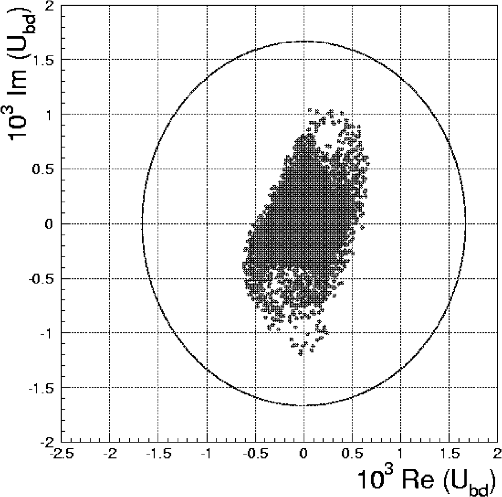
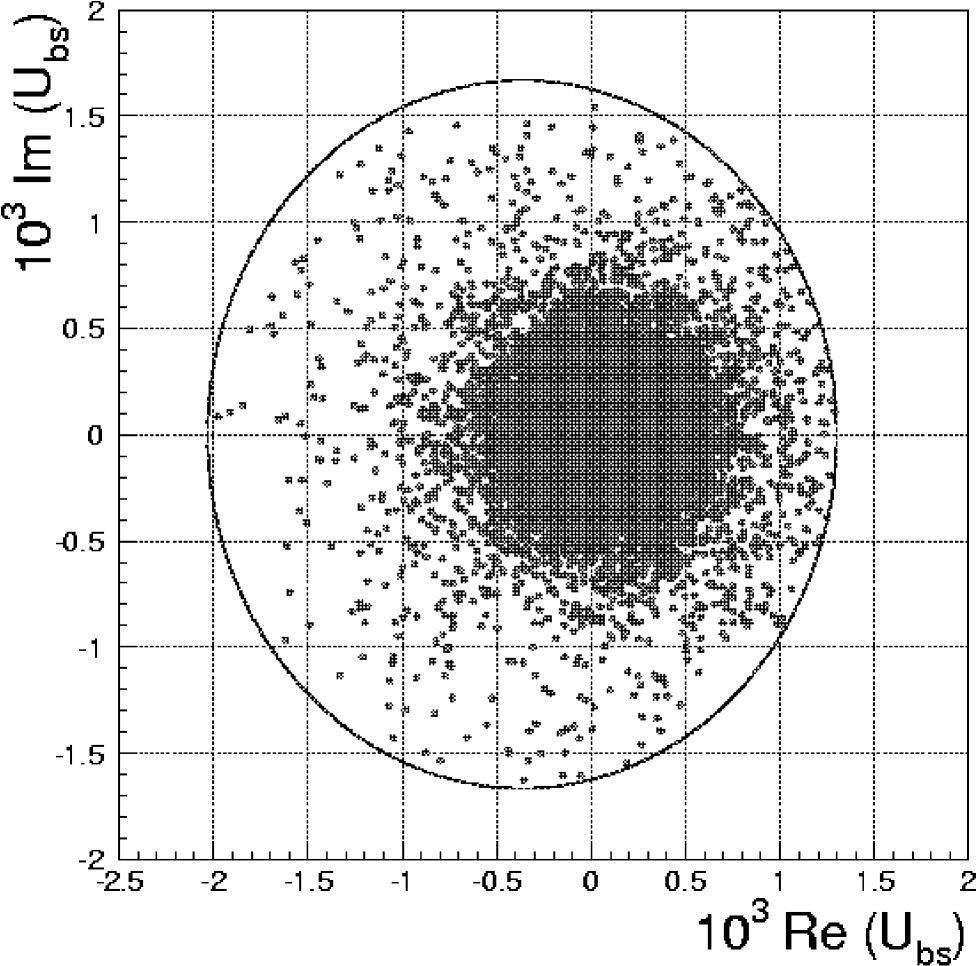
FIG. 1.: Scatter plot of the allowed $U_{bd}$ and $U_{bs}$ with all the constraints described in the text, but no $B^{0}$ CP asymmetry requirement.

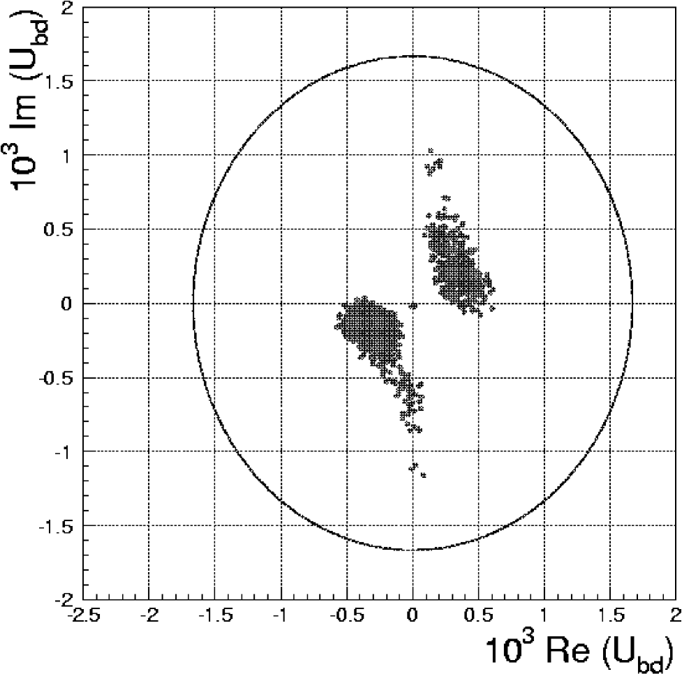
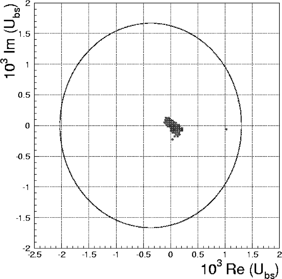
FIG. 2.: The same plot as before with the additional requirement on the $a_{J/\psi}$ CP asymmetry to reproduce the Babar value, $a_{J/\psi}=0.34\pm 0.20$.

REFERENCES

- [1] F. J. Botella and L. Chau, Phys. Lett. B168, 97 (1986).
-
[2]
G. C. Branco and L. Lavoura,
Phys. Lett. B208, 123 (1988);
G. C. Branco and L. Lavoura, Phys. Rev. D38, 2295 (1988). -
[3]
B. Aubert et al. [Babar Collaboration], Report No. SLAC-PUB-8540,
hep-ex/0008048;
B. Aubert et al. [BaBar Collaboration], Phys. Rev. Lett. 86, 2515 (2001) [hep-ex/0102030]. -
[4]
H. Aihara [Belle Collaboration], Belle note 353,
hep-ex/0010008;
A. Abashian et al. [BELLE Collaboration], Phys. Rev. Lett. 86, 2509 (2001) [hep-ex/0102018]. - [5] T. Affolder et al., CDF Collaboration, Phys. Rev. D61, 072005 (2000), hep-ex/9909003.
-
[6]
J. P. Silva and L. Wolfenstein, Report No. SLAC-PUB-8548,
hep-ph/0008004;
G. Eyal, Y. Nir and G. Perez, JHEP 0008, 028 (2000), hep-ph/0008009;
Z. Xing, hep-ph/0008018;
A. J. Buras and R. Buras, Report No. TUM-HEP-285-00, hep-ph/0008273;
A. Masiero and O. Vives, Report No. SISSA-69-2000-EP, to be published in Phys. Rev. Lett., hep-ph/0007320;
A. Masiero, M. Piai and O. Vives, Report No. FTUV-12-08, hep-ph/0012096. -
[7]
F. del Aguila and J. Cortes,
Phys. Lett. B156, 243 (1985);
G. C. Branco and L. Lavoura, Nucl. Phys. B278, 738 (1986);
F. del Aguila, M. K. Chase and J. Cortes, Nucl. Phys. B271, 61 (1986);
Y. Nir and D. J. Silverman, Phys. Rev. D42, 1477 (1990);
D. Silverman, Phys. Rev. D45, 1800 (1992);
G. C. Branco, T. Morozumi, P. A. Parada and M. N. Rebelo, Phys. Rev. D48, 1167 (1993);
W. Choong and D. Silverman, Phys. Rev. D49, 2322 (1994);
V. Barger, M. S. Berger and R. J. Phillips, Phys. Rev. D52, 1663 (1995), hep-ph/9503204;
D. Silverman, Int. J. Mod. Phys. A11, 2253 (1996), hep-ph/9504387;
M. Gronau and D. London, Phys. Rev. D55, 2845 (1997), hep-ph/9608430;
F. del Aguila, J. A. Aguilar-Saavedra and G. C. Branco, Nucl. Phys. B510, 39 (1998), hep-ph/9703410. - [8] L. Chau and W. Keung, Phys. Rev. Lett. 53, 1802 (1984).
- [9] D. E. Groom et al., Eur. Phys. J. C15, 1 (2000).
- [10] L. Lavoura and J. P. Silva, Phys. Rev. D47, 1117 (1993).
- [11] F. del Aguila, J. A. Aguilar-Saavedra and R. Miquel, Phys. Rev. Lett. 82, 1628 (1999), hep-ph/9808400.
- [12] A. J. Buras and L. Silvestrini, Nucl. Phys. B546, 299 (1999), hep-ph/9811471.
-
[13]
D. Gomez Dumm and A. Pich,
Phys. Rev. Lett. 80, 4633 (1998),
hep-ph/9801298;
G. D’Ambrosio, G. Isidori and J. Portoles, Phys. Lett. B423, 385 (1998), hep-ph/9708326. - [14] T. Inami and C. S. Lim, Prog. Theor. Phys. 65, 297 (1981).
- [15] A. J. Buras and R. Fleischer, Report No. TUM-HEP-275-97, hep-ph/9704376.
-
[16]
M. Ciuchini, E. Franco, L. Giusti, V. Lubicz and G. Martinelli,
Report No. ROME-99-1268,
hep-ph/9910237;
M. Ciuchini and G. Martinelli, Report No. TUM-HEP-376-00, hep-ph/0006056;
S. Bosch, A. J. Buras, M. Gorbahn, S. Jager, M. Jamin, M. E. Lautenbacher and L. Silvestrini, Nucl. Phys. B565, 3 (2000), hep-ph/9904408. -
[17]
S. Bertolini, J. O. Eeg, M. Fabbrichesi and E. I. Lashin,
Nucl. Phys. B514, 93 (1998),
hep-ph/9706260;
S. Bertolini, M. Fabbrichesi and J. O. Eeg, Rev. Mod. Phys. 72, 65 (2000), hep-ph/9802405. - [18] E. Pallante and A. Pich, Phys. Rev. Lett. 84, 2568 (2000), hep-ph/9911233.
- [19] Y. Nir, Report No. IASSNS-HEP-99-96, hep-ph/9911321.
- [20] G. Barenboim and F. J. Botella, Phys. Lett. B433, 385 (1998), hep-ph/9708209.
- [21] G. Eyal and Y. Nir, JHEP 9909, 013 (1999), hep-ph/9908296.
- [22] S. Glenn et al. [CLEO Collaboration], Phys. Rev. Lett. 80, 2289 (1998), hep-ex/9710003.
- [23] G. Buchalla, G. Hiller and G. Isidori, Report No. SLAC-PUB-8430, hep-ph/0006136.
- [24] G. Barenboim, F. J. Botella, G. C. Branco and O. Vives, Phys. Lett. B422, 277 (1998), hep-ph/9709369.
- [25] G. Barenboim, G. Eyal and Y. Nir, Phys. Rev. Lett. 83, 4486 (1999), hep-ph/9905397.