Abstract

We have investigated the evolution of the neutrino asymmetry in active-sterile neutrino oscillations in the early universe. We find that there are large regions of parameter space where the asymmetry is extremely sensitive to variations in the initial asymmetry as well as the external parameters (the mass difference and the mixing angle). In these regions the system undergoes chaotic transitions; however, the system is never truly chaotic in the sense that all information about initial conditions is lost. In some cases though, enough information is lost that the final sign of the neutrino asymmetry is stochastic. We discuss the implications of our findings for Big Bang nucleosynthesis (BBN) and the cosmic microwave background (CMB).

Neutrino oscillations have been proven beyond reasonable doubt by the observation of the solar and atmospheric neutrino anomalies. The solar neutrino problem can be explained by oscillations between $\nu_{e}$ and $\nu_{\mu}$ [1], whereas the atmospheric neutrino deficit is quite nicely explained by oscillations between $\nu_{\mu}$ and $\nu_{\tau}$ [2]. However, the LSND experiment also claims detection of neutrino oscillations between $\nu_{\mu}$ and $\nu_{e}$, but with a much larger mass difference than found from the solar neutrino experiments [3]. There is no possible three-neutrino solution to the combined data. Either one of the interpretations is wrong, or there is a fourth neutrino species, responsible for either the atmospheric or the solar neutrino anomaly. It has proven difficult to rule out the existence of such a fourth neutrino. It cannot interact via the usual weak interactions, or it would have been detected in $Z$-decay experiments. However, such additional light sterile neutrinos are predicted to exist in many extensions of the standard model, and it is certainly worthwhile to study the implications of such neutrinos for cosmology.

Active-sterile neutrino oscillations in the early universe have been intensely studied for more than a decade. The pioneering studies concentrated on effects from excitation of inert degrees of freedom from the background plasma on BBN predictions of the abundances of the light elements [4-10]. Extra degrees of freedom exited before the BBN epoch increases the relativistic energy density of the universe. This modifies the expansion rate of the universe and changes the outcome of BBN, most notably the primordial helium abundance, $Y_{P}$.

It was realized early on that neutrino oscillations in a CP asymmetric plasma like the early universe could amplify an initial neutrino asymmetry $(L_{\nu}\equiv(N_{\nu}-N_{\bar{\nu}})/N_{\gamma})$ [5]. Initially, the effect was thought unimportant [7], and it was not until 1996 where Foot, Thomson and Volkas [11] showed that for for some mixing parameters, an important and non negligible asymmetry can actually be generated and affect BBN-predictions [11, 12]. These results were confirmed by Shi [13], who in addition argued that in parts of the $(\delta m^{2},\sin 2\theta)$-parameter space, the sign of the asymmetry can go though a period of rapid oscillations before settling down at a final value. The magnitude of the final asymmetry seems quite robust, but the final sign is very sensitive to small changes in the initial asymmetry and the mixing parameters. These results have later been investigated in further detail.

Based on the quantum rate equations (QRE’s), Enqvist et al. [14] have confirmed Shi’s results The set of QRE’s is an approximation to the full quantum kinetic equations (QKE’s) for the system, based on the assumption that all modes have the average momentum, $p=\langle p\rangle\simeq 3.15T$. This approximation is excellent outside resonance regions, but its applicability inside resonances has been questioned. The reason is that in the QKE’s different momentum modes pass through the resonance at different temperatures. Assuming only one mode could possibly lead to different behaviour of the oscillations inside the resonance.

Unfortunately it is not yet possible to solve the full QKE’s through a strong resonance due to numerical limitations [15, 16]. This fact has lead to recent controversy about the behaviour of the asymmetry when the full set of QKE’s is employed. We have chosen to work with the quantum rate equations in the present treatment because the equations are numerically solvable and reliable conclusions can be drawn from them. However, we caution that some of our conclusions do not necessarily apply to the full set of quantum kinetic equations.

The question of chaoticity is important since chaotic generation of lepton number might lead to the formation of leptonic domains. Not causally connected regions could develop different signs on the leptonic asymmetry. Diffusion of neutrinos over leptonic boundaries would be expected to suppress asymmetry and might also open a new channel of producing sterile neutrinos via resonant MSW conversion of active neutrinos at domain boundaries [19]

Our goal is to investigate to what extend the final sign of the asymmetry can be stochastic. In order to do this we employ a Lyapunov-exponent analysis of the system and calculate the loss of information about initial conditions experienced as the system passes through the resonance. Finally, we discuss the implications of our findings for BBN and the CMBR.

Equations — The two-neutrino mixing is characterised by the vacuum mixing angle $\theta$. The matter eigenstates $\nu_{1,2}$ are connected to the flavor eigenstates $\nu_{\alpha,s}$ via the transformations

$$\nu_{\alpha} = \cos\theta\,\nu_{1}-\sin\theta\,\nu_{2}$$

$$\nu_{s} = \sin\theta\,\nu_{1}+\cos\theta\,\nu_{2}.$$ (1)

If the two mass eigenstates have masses $m_{1}$ and $m_{2}$, the squared mass difference is defined as; $\delta m^{2}=m_{2}^{2}-m_{1}^{2}$. The objects of interest are the reduced 2$\times$2-density matrices $\rho_{\nu}$ and $\rho_{\overline{\nu}}$ for the neutrino and anti-neutrino ensembles respectively. Expanded in [7, 20] Pauli spin matrices these take the form

$$\rho_{\nu}=\frac{1}{2}P_{0}(1+\mathbf{P}\cdot\sigma);\qquad\rho_{\overline{\nu}}=\frac{1}{2}\overline{P}_{0}(1+\mathbf{\overline{P}}\cdot\sigma).$$ (2)

The coefficients in the expansion form the components of the polarisation vector $\mathbf{P}$.

The diagonal elements in $\rho_{\nu}$ are the relative number densities of the active neutrino and the sterile neutrinos normalised to their equilibrium values

$$n_{\nu_{\alpha}}=\frac{1}{2}P_{0}(1+P_{z}),\qquad n_{\nu_{s}}=\frac{1}{2}P_{0}(1-P_{z})$$ (3)

with similar equations for the antineutrino ensemble. With the adopted normalisation, $P_{0}$ then equals the sum of the relative number densities of the mixed neutrinos (2 in chemical equilibrium). $P_{z}$ measures the distribution between the active and the sterile neutrinos. If $P_{z}$=1 all neutrinos in the mixed ensemble will be of the active type, whereas all neutrinos will be of the sterile type if $P_{z}=-1$.

Instead of solving the full set of QKE’s for $\rho_{\nu}(p)$ and $\rho_{\bar{\nu}}(p)$, we solve the quantum rate equations for $\rho_{\nu}(p=\langle p\rangle)$ and $\rho_{\bar{\nu}}(p=\langle p\rangle)$, where $\langle p\rangle\simeq 3.15T$ .

We focus on the part of parameter space where the the final sign of the leptonic asymmetry appears extremely sensitive towards small changes in the parameters. In this part of parameter space collision terms can be neglected so that the resonance is non-adiabatic and no significant amount of sterile neutrinos are produced. $P_{0}$ is then a constant which can be put equal to unity. The approximation is valid for mixing parameters obeying the inequality [9]

$$|\delta m^{2}|\sin^{4}2\theta<10^{-9}.$$ (4)

The coupled equations of motion then are

$$\dot{\mathbf{P}}=\mathbf{V}\times\mathbf{P}-D\cdot\mathbf{P_{T}},\qquad\dot{\mathbf{\overline{P}}}=\mathbf{\overline{V}}\times\mathbf{\overline{P}}-\overline{D}\cdot\mathbf{\overline{P}_{T}},$$ (5)

where $\dot{\mathbf{P}}\equiv d\mathbf{P}/dt$, and the transversal polarisation vector $\mathbf{P_{T}}\equiv$ $P_{x}$ $\hat{\mathbf{x}}+P_{y}\hat{\mathbf{y}}$ has been introduced. For definiteness we shall here focus on $\nu_{\tau}-\nu_{s}$ oscillations; other cases are obtained from this by simple redefinitions. The damping coefficient $D$ signifies quantum damping introduced in the system by coherent and incoherent scattering of neutrinos on particles in the background plasma. In the case of $\nu_{\tau}-\nu_{s}$ oscillations it is given by [8, 20]

$$D\simeq\overline{D}\simeq 1.83\,G_{F}^{2}T^{5}\simeq 2.49\times 10^{-46}\,T^{5}\textrm{ eV}^{-4}.$$ (6)

The rotation or potential vector $\mathbf{V}$ arises from an expansion of the total weak Hamiltonian in Pauli spin matrices. In the case of $\nu_{\tau}-\nu_{s}$ oscillations it is given by

$$\mathbf{V}=-b_{s}\,\mathbf{\hat{x}}+(-b_{c}-V_{\nu_{\tau}})\,\mathbf{\hat{z}},\qquad\mathbf{\overline{V}}=-b_{s}\,\mathbf{\hat{x}}+(-b_{c}-\overline{V}_{\nu_{\tau}})\,\mathbf{\hat{z}},$$ (7)

where

$$b_{s}=-\frac{\sin 2\theta\,\delta m^{2}}{2\langle p\rangle}\simeq-\frac{\sin 2\theta\,\delta m^{2}}{6.3\,T},$$ (8)

and

$$b_{c}=-\frac{\cos 2\theta\,\delta m^{2}}{2\langle p\rangle}\simeq-\frac{\cos 2\theta\,\delta m^{2}}{6.3\,T}.$$ (9)

The term $V_{\nu_{\tau}}$($\overline{V}_{\nu_{\tau}}$) is an effective energy contribution to the $\nu_{\tau}$($\overline{\nu}_{\tau}$) from neutral current and charged current interactions with particles in the background. It is given by [21, 8]

$$V_{\tau}=-b_{T}+b_{A}\delta P_{z},\qquad\overline{V}_{\tau}=-b_{T}-b_{A}\delta P_{z}$$ (10)

The parameter $b_{T}$ is the contribution to the effective potential from the low energy tail of the vector bosons

$$b_{T}=\frac{4\sqrt{2}\xi(3)}{\pi^{2}}\frac{\cos^{2}\theta_{W}\langle p\rangle^{2}}{M_{W}^{2}}G_{F}T^{3}=9.36\times 10^{-45}\ \textrm{eV}^{-4}\,T^{5}.$$ (11)

The second term in Eq. (10) is a matter potential arising in an asymmetric background. The parameter $b_{A}$ is given by

$$b_{A}=\frac{3\sqrt{2}\xi(3)}{4\pi^{4}}G_{F}T^{3}\simeq 1.53\times 10^{-24}\ \textrm{eV}^{-2}\,T^{3}$$ (12)

and we have defined the parameter

$$\delta P_{z}=\frac{8}{3}L^{(\tau)}.$$ (13)

The term $L^{(\mu,\tau)}$ contains all the asymmetries in the problem

$$L^{(\tau)}=2L_{\nu_{\tau}}+L_{\nu_{\mu}}+L_{\nu_{e}}-\frac{1}{2}L_{n}.$$ (14)

An asymmetry is defined as $L_{\nu_{\alpha}}=(N_{\nu_{\alpha}}-N_{\overline{\nu}_{\alpha}})/N_{\gamma}$, where $N_{\nu_{\alpha}}=(3/8)N_{\gamma}n_{\nu_{\alpha}}$ is the number density of a given neutrino specie and $N_{\gamma}=2\xi(3)T^{3}/\pi^{2}$ is the photon number density. Specifically for $\nu_{\tau}$ one finds

$$L_{\nu_{\tau}}=\frac{3}{8}(P_{z}-\overline{P}_{z}),$$ (15)

such that

$$\delta P_{z}=P_{z}-\overline{P}_{z}+P_{c},$$ (16)

where $P_{c}=(8/3)L^{\rm in}$ is a constant initial asymmetry.

The expansion of the universe is given by the Friedmann equation $H=\sqrt{8\pi G\rho/3}$, where $\rho=\frac{\pi^{2}}{30}g_{*}T^{4}$. In accordance with our assumption of non-adiabatic oscillations we take $g_{*}=Const=10.75$ [22].

Since we are focusing on the evolution of small asymmetries it is an advantage to redefine the polarisation vectors ($\mathbf{P}$ and $\mathbf{\overline{P}}$) as

$$P_{i}^{\pm}=P_{i}\pm\overline{P}_{i}\qquad(i=x,y,z).$$ (17)

in order to separate small $(P^{-})$ and large $(P^{+})$ quantities. This greatly increases the numerical accuracy.

Numerical results — We have numerically studied the system of equations at temperatures below 100 MeV. At high temperatures the $\nu_{\tau}$ will be in thermal equilibrium via its weak interactions. The $\nu_{s}$ can only be brought into thermal equilibrium by oscillations. However, at high temperatures the damping is very strong and oscillations therefore totally washed out. Initially the abundance of $\nu_{s}$ will therefore be practically zero. The initial lepton asymmetry is plausible comparable in magnitude to the baryon asymmetry $(L^{\rm in}\sim 10^{-10}-10^{-9}$ (however, this need not be the case). The evolution of the leptonic asymmetry depends upon the sign of $\delta m^{2}$. If $\delta m^{2}<0$ the system encounters a MSW resonance where the effective matter mixing angle becomes maximal at a temperature (see e.g. [13])

$$T_{\rm res}=16.0\left(\cos 2\theta\cdot(|\delta m^{2}|/\textrm{eV}^{2})\right)^{1/6}\textrm{ MeV}.$$ (18)

We find solutions very similar to those discussed by Enqvist et al.[14]. We also find that in large regions of parameter space the sign of the final asymmetry is extremely sensitive to small variations in mixing parameters and initial asymmetry. It is interesting to investigate if the observed sign indeterminacy is a real chaotic phenomenon in the mathematical sense that all information about the initial condition is lost during the process of asymmetry amplification or if the system is just “sensitive”.

In order to investigate these dynamical aspects of the system, we have numerically calculated the Lyapunov characteristic exponents, $\lambda_{i}$ (LCE’s). The LCE’s measure the exponential divergence and convergence of nearby orbits in phase space. A dissipative system with a positive LCE is defined as chaotic since it ultimately losses all information about the initial condition. A dissipative system contracts phase space volume in time $(\sum\lambda_{i}<0)$. The set of QRE’s is a dissipative dynamical system because of the expansion of the universe, so that the LCE’s is an ideal way to study the properties of the system.

$\lambda_{i}>0$ is not only a necessary condition for chaos, it also quantifies the degree of chaos in the system. Its magnitude is a measure of how long it takes for an initial uncertainty do develop into total chaos. The information loss $I$ related to a postive LCE is basicly after a time $t$ equal to $I=\lambda t$ and is typically measured in bits.

We have numerically calculated the LCE’s for the QRE’s (5). The calculation has been based on a method by Benettin [23, 24]. An orbit in 6-dimensional phase-space is defined by integrating the non-linear system of 6 QRE’s. Surrounding an initial point on this reference orbit is fixed a sphere defined by 6 principal axes. The surface of this sphere now defines the different initial conditions in the problem. When integrating the non-linear system forward in time the sphere follows the point on the reference orbit that it is fixed to. While doing this it becomes deformed to a 6-ellipsoid because of the divergence or convergence of close orbits in phase-space. We define the LCE’s from the change in the magnitude of the lengths $|\vec{v}_{i}|$ of the spheres’ principal axes

$$\lambda_{i}=\lim_{t\to\infty}\,\frac{1}{t}\,\log_{2}\frac{|\vec{v}_{i}(t)|}{|\vec{v}_{i}(0)|},$$ (19)

The evolution of the sphere’s principal axes is defined by a linearised version of the non liniar set of equations. In each integration point the magnitude of the sphere’s principal axes are compared to the magnitude at the previous integration point. Averaged over time this produces the time averaged LCE’s [23].

The system of 6 QRE’s contains 6 different LCE’s. Until the system hits the resonance all 6 exponents are negative and no information lost. Once the system encounters the resonance, the leptonic asymmetry begins to oscillate rapidly from positive to negative values. At this point the dynamics of the system changes; it now has 1 positive and 5 negative exponents, so information is lost. Fig. 1 has been produced form the initial conditions ($\delta m^{2}$, $\sin^{2}2\theta$, $P_{c}$)=($-10^{-3}\textrm{ eV}^{2}$, $10^{-5}$, $10^{-10}$). The upper panel shows the asymmetry as a function of temperature inside the resonance, whereas the lower displays the loss of information through the resonance. This information loss has been averaged over 100 different initial conditions which lie very close in phase space. This eliminates noise and does not in any way distort the conclusions.

The LCE’s in general depend upon the initial conditions. Only if an ergodic measure exists for the attractor, will almost all initial conditions in the basin of attraction result in the same LCE’s [27]. Often, the structure of the basin of attraction is so complicated that even a small variation in initial conditions puts one in the basin of attraction of another attractor, characterized by a different set of LCE’s [25].

Figure 1: Upper panel: The evolution of $L_{\nu}$ with temperature for the parameters $\delta m^{2}=-10^{-3}\,{\rm eV}^{2}$, $\sin^{2}2\theta=10^{-5}$ and $L_{\nu}^{\rm in}=10^{-10}$. Lower panel: The total loss of information in bits for the same model.

In Fig. 1 it seems reasonable that the situation with a negative final asymmetry can not be characterized by the same attractor as the situation with a positive final asymmetry. Most likely a different type of attractor also appears when the system crosses the resonance, namely a chaotic attractor [26]. Since different attractors in general are characterized by different LCE’s, one must average the LCE’s over different initial conditions to probe the spatial structure of the attractor.

From Fig. 1 it is noticed that as the asymmetry initially grows and starts oscillating rapidly, information is lost. After the initial violent growth the lepton number oscillates more regularly, and information is no longer lost. Very suddenly the system begins then to oscillate with much smaller amplitude around one of the two attractors. This can be considered a chaotic transition where, as displayed in the lower part of Fig. 1, information is rapidly lost. The system goes through this alternating behaviour of ”ordinary oscillations“ followed by chaotic transitions all the way trough the resonance. However, ultimately the system is driven out of the chaotic region by the expansion of the universe such that only a limited amount of information is lost.

Figure 2: Upper panel: The evolution of $L_{\nu}$ with temperature for the parameters $\delta m^{2}=-10^{-3}\,{\rm eV}^{2}$, $\sin^{2}2\theta=10^{-7}$ and $L_{\nu}^{\rm in}=10^{-10}$. Lower panel: The total loss of information in bits for the same model.

The system is not truly chaotic in the sense that it has a positive time averaged Lyapunov exponent at all times. However, it goes trough the chaotic region and will therefore be sensitive to variations in initial conditions. This sensitivity depends on the amount of information lost, which again depends critically on the value of the mixing parameters. Fig. 2 has been produced from the initial conditions ($\delta m^{2}$, $\sin^{2}2\theta$, $P_{c}$)=($-10^{-3}\textrm{ eV}^{2}$, $10^{-7}$, $10^{-10}$) and illustrates nicely that the loss of information is smaller for smaller mixing angles.

In general we find that the sensitivity grows with larger mixing angles and smaller mass differences. This is clearly seen in Fig. 3 where we have calculated the total loss of information (in bits) for different values of $\delta m^{2}$ and $\sin^{2}2\theta$.

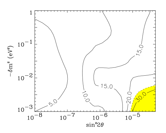
Figure 3: The loss of information, calculated for different values of $\delta m^{2}$ and $\sin^{2}2\theta$. In all cases we have assumed an initial asymmetry of $L_{\nu}^{\rm in}=10^{-10}$.

Discussion — We have performed a careful study of the dynamical properties of the quantum rate equations for active-sterile neutrino oscillations in the early universe. Numerically we have confirmed the results of Ref. [14], that there are regions of parameter space where the final sign of the lepton asymmetry is extremely sensitive to initial conditions. However, even though the systems goes through chaotic transitions, it is never truly chaotic in a mathematical sense because the system only stays a finite time in the chaotic regions.

Effectively though, the system can behave exactly like a chaotic system in some regions of parameter space. Thermal fluctuations in the early universe can be expected to produce slightly different initial asymmetries, of the order $\Delta L^{\rm in}\simeq 10^{-18}$ [15]. If the average initial asymmetry is of the order $L^{\rm in}\simeq 10^{-10}$ the information loss needs only be of the order 25 bits in order to produce a completely arbitrary final sign. We have indicated this region of $(\delta m^{2},\sin^{2}2\theta)$-space in Fig. 3 by a light shading.

It should be noted that there are reasons for believing that much larger initial differences in $L$ could be present. They could for instance have been produced during the electroweak phase transition (there could be cases where $\Delta L^{\rm in}\simeq L^{\rm in}$). In that case, large regions in the mixing parameter space leads to arbitrary sign, essentially the asymmetry only has to go through a few oscillations.

The outcome of BBN depends strongly on the sign of a possible lepton asymmetry, if the asymmetry is in the electron neutrino sector. The reason is that electron neutrinos participate directly in the weak reactions that interconvert neutrons and protons. A positive $L$ leads to an decrease in $Y_{P}$ and a negative $L$ to an increase. So in principle different regions could have different light element abundances. The uncertainty in $Y_{P}$ is expected to be of the order $10^{-2}$. The formation of domains with different lepton number can in principle also lead to visible effects in the CMB. The extra energy density produced by repopulation is in most cases very small (which is exactly why our non-adiabatic approximation applies), so the oscillations are not detectable in this way [28]. However, the recombination history depends sensitively on $Y_{P}$, so the CMB anisotropies are still altered to some extent by the oscillations.

Finally, we caution that our calculations have been performed using the quantum rate equations (QRE’s) instead of the full set of quantum kinetic equations (QKE’s). The interaction between different momentum states has been neglected in the QRE’s and it is likely that a full solution of the QKE’s would find a somewhat smaller degree of chaos. However, it also seems well-established that the asymmetry does indeed oscillate also when the QKE’s are solved [15, 16], and so one may expect our analysis to qualitatively also apply to the QKE’s.

Acknowledgements — One of us (PEB) wishes to thank Nordita, where this work was completed, for hospitality.

References

- [1] J. N. Bahcall, P. I. Krastev and Yu. Smirnov, Phys. Rev. D 58 (1998) 096016; Phys. Rev. D 60 (2000) 93001.
- [2] Y. Fukada et al., Phys. Rev. Lett. 81 (1998) 1562.
- [3] C. Athanassopoulos et al., Phys. Rev. C 54 (1996) 2685; Phys. Rev. C 58 (1998) 2489; Phys. Rev. Lett. 81 (1998) 1774.
- [4] A. Dolgov, Sov. J. Nucl. Phys. 33 (1981) 700; L. Stodolsky, Phys. Rev. D 36 (1987) 2273.
- [5] R. Barbieri and A. Dolgov, Phys. Lett. B 237 (1990) 440; Nucl. Phys. B 237 (1991) 742.
- [6] K. Kainulainen, Phys. Lett. B 244 (1990) 191; K. Enqvist, K. Kainulainen, J. Maalampi, Phys. Lett. B 244 (1990) 186; Phys. Lett. B 249 (1990) 531; K. Enqvist, K. Kainulainen, M. Thomson, Phys. Lett. B 280 (1992) 498, J. Cline, Phys. Rev. Lett. 68 (1992) 3137.
- [7] K. Enqvist, K. Kainulainen, and J. Maalampi, Nucl. Phys. B 349 (1991) 754.
- [8] K. Enqvist, K. Kainulainen, M. J. Thomson, Nucl. Phys. B 373 (1992) 498.
- [9] X. Shi, D. N. Schramm, B. D. Fields, Phys. Rev. D 48 (1993) 2563.
- [10] R. Foot, R. R. Volkas, Phys. Rev. Lett. 75 (1995) 4350.
- [11] R. Foot, M. J. Thomson and R. R. Volkas, Phys. Rev. D 53 (1996) 5349.
- [12] R. Foot, R. R. Volkas, Phys. Rev. D 55 (1997) 5147; Phys. Rev. D 56 (1997) 6653; D 59 (1999) 029901 (E); X. Shi, G. M. Fuller, K. Abazajian, Phys. Rev. D 60 (1999) 063002.
- [13] X. Shi, Phys. Rev. D 54 (1996) 2753.
- [14] K. Enqvist, K. Kainulainen, A. Sorri, Phys. Lett. B 464 (1999) 199.
- [15] P. Di Bari, R. Foot, Phys. Rev. D 61 (2000) 105012.
- [16] R. R. Volkas, Y. Y. Y. Wong, hep-ph/0007185.
- [17] A. D. Dolgov, S. H. Hansen, S. Pastor, D. V. Semikoz, Astropart. Phys. 14 (2000) 79.
- [18] P. Di Bari, R. Foot, R. R. Volkas, Y. Y. Y. Wong, hep-ph/0008245; R. Buras, D. V. Semikoz, hep-ph/0008263.
- [19] X. Shi, G. M. Fuller, Phys. Rev. Lett. 83 (1999) 3120; P. Di Bari, Phys. Lett. B 482 (2000) 150.
- [20] B. H. J. McKellar, M. J. Thomson, Phys. Rev. D 49 (1994) 2710.
- [21] D. Nötzold, G. Raffelt, Nucl. Phys. B 307 (1988) 924.
- [22] E. W. Kolb, M. S. Turner, The Early Universe, Addison-Wesley Publishing Company (1993).
- [23] A. Wolf, Quantifying chaos with Lyapunov exponents, in Chaos, ed. A. V. Holden, Manchester University Press (1987) 273; A. Wolf, J. B. Swift, H. L. Swinney, J. A. Vastano, Physica D 16 (1984) 285.
- [24] G. Benettin, L. Galgani, A. Giorgilli, J.-M. Strelcyn, Meccanica (1980) 21.
- [25] H. G. Schuster, Deterministic Chaos, an introduction, second revised edition, VCH verlagsgeselschaft (1989).
- [26] E. Ott, Chaos in dynamical systems, Cambridge University Press (1993).
- [27] J.-P. Eckmann, D. Ruelle, Rev. Mod. Phys. 57 (1985) 617.
- [28] S. Hannestad, G. Raffelt, Phys. Rev. D 59 (1998) 043001.