Large lepton mixing and supernova 1987A

Abstract:

We reconsider the impact of $\bar{\nu}_{e}\leftrightarrow\bar{\nu}_{\mu,\tau}$ neutrino oscillations on the observed $\bar{\nu}_{e}$ signal of supernova SN 1987A. Performing a maximum-likelihood analysis using as fit parameters the released binding energy $E_{\rm b}$ and the average neutrino energy $\langle E_{\bar{\nu}_{\rm e}}\rangle$, we find as previous analyses that $\bar{\nu}_{e}\leftrightarrow\bar{\nu}_{\mu,\tau}$ oscillations with large mixing angles have lower best-fit values for $\langle E_{\bar{\nu}_{\rm e}}\rangle$ than small-mixing angle (SMA) oscillations. Moreover, the inferred value of $\langle E_{\bar{\nu}_{\rm e}}\rangle$ is already in the SMA case lower than those found in simulations. This apparent conflict has been interpreted as evidence against the large mixing oscillation solutions to the solar neutrino problem. In order to quantify the degree to which the experimental data favour the SMA over the large mixing solutions we use their likelihood ratios as well as a Kolmogorov-Smirnov test. We find within the range of SN parameters predicted by simulations regions in which the LMA-MSW solution is either only marginally disfavoured or favoured compared to the SMA-MSW solution. We conclude therefore that the LMA-MSW solution is not in conflict with the current understanding of SN physics. In contrast, the vacuum oscillation and the LOW solutions to the solar neutrino problem can be excluded at the $4\sigma$ level for most of the SN parameter ranges found in simulations. Only a marginal region with low values of $\langle E_{\bar{\nu}_{\rm e}}\rangle$, $\langle E_{\bar{\nu}_{\mu,\tau}}\rangle$ and $E_{\rm b}$ is left over, in which these oscillation solutions can be reconciled with the neutrino signal of SN 1987A.

1 Introduction

The impact of neutrino properties beyond the standard model on the observed neutrino signal [1] of supernova (SN) SN 1987A has been discussed in numerous works during the last 13 years. Most of the early works discussed either mass limits for $\nu_{e}$ or the impact of matter-induced oscillations on the prompt $\nu_{e}$ burst [2]. In the latter case the MSW effect in the SN envelope would have rendered the prompt $\nu_{e}$ burst unobservable for a large area of mixing parameters assuming a normal mass hierarchy. On the other hand, the main neutrino signal of SN 1987A which is the $\bar{\nu}_{e}$ pulse detected by the reaction $\bar{\nu}_{e}+p\to n+e^{+}$ is then influenced only for large mixing angles (LMA) by oscillations. It was argued [3, 4] that LMA neutrino oscillations would increase the discrepancy between the observed $\bar{\nu}_{e}$ spectrum and the one predicted by SN simulations [5, 6, 7, 9]. Moreover, the theoretical prejudice was until recently that lepton mixing is, similar to quark mixing, small. Therefore, the small mixing angle SMA-MSW solution to the solar neutrino problem seemed to be favoured both by the neutrino signal of SN 1987A and by theoretical arguments.

Meanwhile, the LMA-MSW solution to the solar neutrino problem has become the best oscillation solution to the solar neutrino problem [10], while Superkamiokande atmospheric neutrino data [11] strongly indicate the need for $\nu_{\mu}\to\nu_{\tau}$ oscillations with maximal or nearly maximal mixing [10]. Such approximate bi-maximal neutrino mixing patterns [12] can actually arise either in theoretical models based on unification ideas [13] or in “bottom-up” models, such as that of Ref. [14]. It is therefore interesting to reconsider how serious the discrepancy between the observed and the predicted $\bar{\nu}_{e}$ spectra of SN 1987A should be taken.

The main goal of this work is not to obtain those values of the neutrino oscillation parameters, $\tan^{2}\vartheta$ and $\Delta m^{2}$, that fit best the neutrino signal from SN 1987A. Instead we use the best-fit points found from solar neutrino data for three [SMA-MSW, LMA-MSW, and vacuum oscillations (VO)] of the four allowed solutions as input and try then to assess to what extend the LMA solutions are (dis-) favoured compared to SMA assuming certain astrophysical parameters. The case of the LOW solution which extends as only one also into the so-called dark side ($\vartheta>\pi/4$) of the solar neutrino problem [15] will be discussed separately. There, we are mainly interested in the question if the dark side is compatible with the neutrino signal from SN 1987A [3, 16]. In all cases, we use as measure for the degree to which the experimental data favour one of the allowed solutions over the others their likelihood ratios as well as a Kolmogorov-Smirnov test.

	SMA	LMA	VO
$\Delta m^{2}$/eV2	$5.0\times 10^{-6}$	$3.2\times 10^{-5}$	$1.0\times 10^{-10}$
$\tan^{2}\vartheta$	0.00058	0.33	0.52

Table 1: Best-fit values for the mass difference squared $\Delta m^{2}$ and the mixing angle for different oscillation solutions to the solar neutrino problem, from Ref. [10].

Our main result is that there is a region in the space of astrophysical parameters (average neutrino energies $\langle E_{i}\rangle$ and released binding energy $E_{\rm b}$) predicted by SN simulations in which the LMA-MSW solution is either only marginally disfavoured or favoured compared to the SMA-MSW solution. For the range of parameters compiled in Ref. [7],

$$14~{}{\rm MeV}\leq\langle E_{\bar{\nu}_{\rm e}}\rangle\leq 17~{}{\rm MeV}$$ (1)

$$24~{}{\rm MeV}\leq\langle E_{\bar{\nu}_{\mu,\tau}}\rangle\leq 27~{}{\rm MeV}$$ (2)

$$1.5\times 10^{53}~{}{\rm erg}\leq E_{\rm b}\leq 4.5\times 10^{53}~{}{\rm erg},$$ (3)

the probability that the LMA-MSW hypothesis is compatible with the detected neutrino signal is extremely varying. We find that for large values of $\langle E_{\bar{\nu}_{\rm e}}\rangle$, $\langle E_{\bar{\nu}_{\mu,\tau}}\rangle$ and $E_{\rm b}$ all three large mixing solutions solutions are practically excluded when compared to the SMA-MSW solution. However the probability that the LMA-MSW hypothesis is compatible with the neutrino signal rises above 10% for values of $\langle E_{\bar{\nu}_{\rm e}}\rangle$, $\langle E_{\bar{\nu}_{\mu,\tau}}\rangle$ and $E_{\rm b}$ near the lower end of (1-3). Moreover, it was recently argued that the average neutrino energies are smaller than earlier believed. For example, nucleon-nucleon bremsstrahlung that has not been included into the earlier supernova codes tends to soften the $\bar{\nu}_{\mu,\tau}$ spectrum [8], a trend which has been confirmed by a recent simulation [9]. This simulation found also for $\langle E_{\bar{\nu}_{\rm e}}\rangle$ a rather low value, $\langle E_{\bar{\nu}_{\rm e}}\rangle\approx 12$ MeV. Since this simulation has not aimed at a self-consistent treatment of the neutrino spectra, the values found therein should be taken only as an indication. If $\langle E_{\bar{\nu}_{\rm e}}\rangle$ is indeed as low as found in Ref. [9], the LMA-MSW solution can be favoured compared to SMA-MSW.

In contrast, the VO and the LOW solutions to the solar neutrino problem can be excluded at the $4\sigma$ level for most of the range of SN parameters found in simulations, and low neutrino energies, $\langle E_{\bar{\nu}_{\rm e}}\rangle\mathrel{\mathop{\kern 0.0pt\hbox to0.0pt{\raise 0.86108pt\hbox{$<$}\hss}}\lower 3.87495pt\hbox{\kern-1.90002pt$\sim$}}12$ MeV and $\langle E_{\bar{\nu}_{\mu,\tau}}\rangle\mathrel{\mathop{\kern 0.0pt\hbox to0.0pt{\raise 0.86108pt\hbox{$<$}\hss}}\lower 3.87495pt\hbox{\kern-1.90002pt$\sim$}}17$ MeV, combined with low $E_{\rm b}$ are required to reconcile these oscillation solutions with the neutrino signal of SN 1987A.

2 Neutrino fluences and oscillations

Massive stars with mass $M\mathrel{\mathop{\kern 0.0pt\hbox to0.0pt{\raise 0.86108pt\hbox{$>$}\hss}}\lower 3.87495pt\hbox{\kern-1.90002pt$\sim$}}8~{}M_{\odot}$ end their lives in spectacular type-II supernova outbursts, releasing almost all their gravitational binding energy via neutrino emission [17]. Numerical simulations [5, 6, 7] as well as analytic considerations [18] show that this energy is approximately equipartioned between the three neutrino flavours. The instantaneous neutrino spectra found in simulations are generally pinched, i.e. their low- and high-energy parts are suppressed relative to a Maxwell-Boltzmann distribution. The pinching of the instantaneous neutrino spectra is however compensated by the superposition of different spectra with decreasing temperatures. Moreover, we have found that the likelihood function depends only weakly on how strongly the spectra are pinched. We present therefore only results using Maxwell-Boltzmann distributions for the time-averaged spectra of the neutrinos. Finally, we assume that the SN emits the same amount of energy in all neutrino flavours.

We perform our analysis in the framework of two-neutrino oscillations $\bar{\nu}_{e}\leftrightarrow\bar{\nu}_{h}=\cos\phi\>\bar{\nu}_{\mu}+\sin\phi\>\bar{\nu}_{\tau}$, which is motivated both by detailed fits of the atmospheric neutrino anomaly [10], but also by the results of the Chooz experiment [19]. Since the energy spectra of $\bar{\nu}_{\mu}$ and $\bar{\nu}_{\tau}$ are identical (up to ${\cal O}(E^{4}G_{F}^{2})$ effects), our results do not depend on $\phi$. The probability of a $\bar{\nu}_{e}$ to arrive at the surface of the Earth can be written as an incoherent sum of probabilities,

$$P_{\bar{e}\bar{e}}=P^{S}_{\bar{e}1}P^{E}_{1\bar{e}}+P^{S}_{\bar{e}2}P^{E}_{2\bar{e}}=\left(1-P_{c}\right)\cos^{2}\vartheta+P_{c}\sin^{2}\vartheta\,,$$ (4)

where $P^{S}_{\bar{e}i}$ denotes the probability that a $\bar{\nu}_{e}$ leaves the star as mass eigenstate $\bar{\nu}_{i}$ and $P^{E}_{i\bar{e}}$ the probability that $\bar{\nu}_{i}$ is detected as $\bar{\nu}_{e}$. The interference terms can be safely neglected for all $\Delta m^{2}$ of interest because of the spread of the neutrino wave packets on their way to the Earth. Deviations from an adiabatic evolution of the neutrino states in the SN envelope are characterised by the crossing probability $P_{c}$. We use as approximation for $P_{c}$ the expression valid for an exponential density profile,

$$P_{c}=\frac{{\rm e}^{-\gamma\cos^{2}\vartheta}-{\rm e}^{-\gamma}}{1-{\rm e}^{-\gamma}}\,,$$ (5)

where the adiabaticity parameter

$$\gamma=\frac{4\pi^{2}l_{\rho}}{l_{\rm osc}}\approx 10^{9}\;\left(\frac{\Delta m^{2}}{{\rm eV}^{2}}\right)\left(\frac{\rm MeV}{E}\right)$$ (6)

is the ratio of density scale height $l_{\rho}$ and neutrino oscillation length $l_{\rm osc}$ in vacuum. The expression (5) has in contrast to the one for a linear density profile the correct non-adiabatic limit, $P_{c}\to\sin^{2}\vartheta$, and describes also for $\gamma>0$ quite accurately the behaviour of $P_{c}$ for a profile typical for a SN envelope, $N_{e}\propto r^{-3}$ [20]. Furthermore, for the case of nearly maximal mixing in which we are especially interested $P_{\bar{e}\bar{e}}=1/2+{\cal O}(\vartheta^{2})$.

The neutrinos from SN 1987A had to cross the mantle of the Earth before they reached the Kam and IMB detectors. Possible matter effects in the Earth can be approximated by a box potential, i.e. by replacing $P^{E}_{i\bar{e}}=|\langle\bar{\nu}_{i}|\bar{\nu}_{e}\rangle|^{2}$ with [3]

$$\cos^{2}\vartheta \to \cos^{2}\vartheta+\sin 2\vartheta^{\prime}\sin(2\vartheta-2\vartheta^{\prime})\sin^{2}(\pi d/l_{\rm osc}^{\prime})$$ (7)

$$\sin^{2}\vartheta \to \sin^{2}\vartheta-\sin 2\vartheta^{\prime}\sin(2\vartheta-2\vartheta^{\prime})\sin^{2}(\pi d/l_{\rm osc}^{\prime})\,,$$ (8)

where primed quantities are evaluated in matter. The distance $d$ traveled through the mantle by the neutrinos and the average density $\rho$ are different for the Kamiokande and IMB detectors. For Kamiokande we use $d=3900$ km and $\rho=3.4$ g/cm³ and for IMB $d=8400$ km and $\rho=4.6$ g/cm³ [3].

Let us now briefly consider the two extreme limits of the general expressions Eqs. (4-8). For small enough $\Delta m^{2}$, neutrino states evolve in the SN envelope strongly non-adiabatically, $\gamma\to 0$ and $P_{c}\to\sin^{2}\vartheta$. Moreover the matter effects in the Earth can be neglected and thus the survival probability becomes identical to the vacuum oscillation probability, $P_{\bar{e}\bar{e}}\to\cos^{4}\vartheta+\sin^{4}\vartheta$. In the opposite limit, the evolution of the neutrino states in the SN envelope is completely adiabatic, $\gamma\to\infty$ and $P_{c}\to 0$. Thus

$$P_{\bar{e}\bar{e}}=P^{S}_{\bar{e}1}P^{E}_{1\bar{e}}=\cos^{2}\vartheta+\sin 2\vartheta^{\prime}\sin(2\vartheta-2\vartheta^{\prime})\sin^{2}(\pi d/l_{\rm osc}^{\prime})\,.$$ (9)

Hence, Eqs. (4-5) describe correctly the survival probability of $\bar{\nu}_{e}$ neutrinos in the region of parameters favoured by the LMA-MSW and the VO solution to the solar neutrino problem and interpolate smoothly for intermediate values of $\Delta m^{2}$ and $\vartheta$. The $\bar{\nu}_{e}$ fluence arriving at the detectors is then

$$F_{\bar{\nu}_{e}}=P_{\bar{e}\bar{e}}F_{\bar{\nu}_{e}}^{0}+(1-P_{\bar{e}\bar{e}})F_{\bar{\nu}_{h}}^{0}$$ (10)

where $F_{\bar{\nu}}^{0}$ stands for the time-integrated flux of neutrinos emitted by the SN.

3 Likelihood analysis

The maximum-likelihood method is a particularly well-suited tool for problems like the one at hand, where we want to extract the maximal possible information from only 19 neutrino events. We test with the likelihood function

$${\cal L}(\alpha)\propto\exp\left(-\int n(E,\alpha)\;dE\right)\prod_{i=1}^{N_{\rm obs}}n(E_{i},\alpha)$$ (11)

the hypothesis that a prescribed neutrino fluence $F_{\bar{\nu}_{e}}(E_{\bar{\nu}_{e}},\alpha)$ leads to the observed experimental data $E_{i}$ with probability distribution $n(E,\alpha)$. The maximisation of ${\cal L}(\alpha)$ gives an estimate of the values $\alpha_{\ast}=\{\tan^{2}\vartheta,\Delta m^{2},E_{\rm b},\langle E_{\bar{\nu}_{\rm e}}\rangle,\langle E_{\bar{\nu}_{\rm h}}\rangle,\ldots\}$ which best represent the data set $E_{i}$. The confidence region around $\alpha_{\ast}$ which contains the true value of $\alpha$ with a specified probability $\beta$ for $k$ fit parameters is given by

$$\ln{\cal L}(\alpha_{\ast})-\ln{\cal L}(\alpha)\leq\frac{1}{2}\chi^{2}_{\beta;k}\,,$$ (12)

if ${\cal L}(\alpha)$ is assumed to be Gaussian near its extrema.

Apart from parameter estimation given a specific hypothesis, the likelihood analysis can also be used to decide which hypothesis fits better the experimental data. In this case, the ratio of the likelihood functions for the different hypotheses is a useful estimator. We will present the best-fit values for a given oscillation hypothesis in Sec. 3.1, while we test which hypothesis fits better the data given a certain range of parameters in Sec. 3.2.

The connection between the observed data set $E_{i}$ and the emitted neutrino fluence $F_{\bar{\nu}_{e}}(E_{\bar{\nu}_{e}},\alpha)$ has been described already in detail in the literature. We follow here closely Ref. [4], but use for the detector efficiencies the fit functions given by Burrows [5].

3.1 Best-fit values and confidence regions

In this subsection we review the best-fit values and confidence regions obtained from our likelihood analysis for the different oscillation hypotheses. Since the likelihood function we use is identical to the one of Ref. [4], our results differ only slightly owing to small shifts of the best-fit values of the solar neutrino data indicated by the most recent analysis [10]. Therefore we present only briefly the main points of this analysis.

In the following, the region of SN parameters (1-3) given in Ref. [7] corresponds always to the cross hatched region in the figures, while the lower values of $\langle E_{\bar{\nu}_{\rm e}}\rangle$ found in Ref. [9] are shown as hatched region. The best-fit values obtained for the three different oscillation hypotheses are summarized in Table 2.

The presence of $\bar{\nu}_{e}\leftrightarrow\bar{\nu}_{\mu,\tau}$ neutrino oscillations can affect the average energy of $\bar{\nu}_{e}$. We have parameterised the $\bar{\nu}_{h}$ energy as $\langle E_{\bar{\nu}_{\rm h}}\rangle=\tau\langle E_{\bar{\nu}_{\rm e}}\rangle$. In Fig. 1, we show the 95.4% C.L. likelihood contour for the LMA-MSW oscillation hypothesis in the $E_{\rm b}$-$\langle E_{\bar{\nu}_{\rm e}}\rangle$ plane. The neutrino oscillation parameters are given in Table 1 and the average energy of $\bar{\nu}_{h}$ is specified by the parameter $\tau$. The case $\tau=1$ corresponds to the Standard Model or SMA-MSW oscillations, because in both cases oscillations can be neglected altogether. The best-fit point is shifted to smaller values of $\langle E_{\bar{\nu}_{\rm e}}\rangle$ for increasing values of $\tau$, and the 95.4% C.L. likelihood contour includes a large portion of the hatched region for $\tau=1.4$ and 1, but only touches it for $\tau=1.7$. Parts of the cross-hatched region (1-3) are however included by none of the oscillation hypotheses, and only in the case of the SMA-MSW solution the 95.4% C.L. likelihood contour touches nearly the boundary of (1-3).

Figure 1: Contours of 95.4% C.L. likelihood for the LMA-MSW oscillation hypothesis as function of $E_{\rm b}$ and $\langle E_{\bar{\nu}_{\rm e}}\rangle$ for $\tau=1,1.4,1.7$ and 2. The best-fit points are marked by crosses.

In Fig. 2, we show the same plot for the VO hypothesis. The oscillation parameters are again given in Table 1. The shift of the best-fit point towards smaller values of $\langle E_{\bar{\nu}_{\rm e}}\rangle$ is now more pronounced and already for $\tau=1.4$ the 95.4% C.L. likelihood contour does not include $\langle E_{\bar{\nu}_{\rm e}}\rangle\approx 12$ MeV. If the VO solution is really realized in Nature, then the SN 1987A data would indeed strongly favour smaller neutrino temperatures as it is usually assumed.

Figure 2: Contours of 95.4% C.L. likelihood for the VO oscillation hypothesis as function of $E_{\rm b}$ and $\langle E_{\bar{\nu}_{\rm e}}\rangle$ for $\tau=1,~{}1.4,~{}1.7$ and 2. The best-fit points are marked by crosses.

	Kam		IMB		joint
	$\langle E_{\bar{\nu}_{e}}\rangle$	$E_{\rm b}$	$\langle E_{\bar{\nu}_{e}}\rangle$	$E_{\rm b}$	$\langle E_{\bar{\nu}_{e}}\rangle$	$E_{\rm b}$	$\Delta\chi^{2}$
SMA	7.8	5.3	11.3	4.8	10.9	3.4	1.9
LMA, $\tau=1.4$	6.6	6.6	9.9	5.8	9.8	3.6	2.0
LMA, $\tau=1.7$	5.6	8.8	7.2	16.2	8.5	4.5	1.6
LMA, $\tau=2$	4.8	10.8	5.9	23.6	7.1	5.9	0.8
VO,  $\tau=1.4$	6.0	6.6	8.4	7.3	8.6	3.9	1.2
VO,  $\tau=1.7$	5.1	7.3	6.9	8.3	7.1	4.5	0.4
VO,  $\tau=2$	4.2	8.7	5.7	9.9	5.9	5.3	0

Table 2: Best fit values for $\langle E_{\bar{\nu}_{\rm e}}\rangle$/MeV and $E_{\rm b}/10^{53}$ erg; both for a separate and a joint analysis of the two experiments. The difference $\Delta\chi^{2}$ of the local minima to the global minimum (VO solution with $\tau=2$) is also given.

The compatibility of the two data sets of Kamiokande and IMB has been already discussed extensively in the literature. Recently, it has been speculated that the LMA-MSW solution can improve the agreement between the two experiments [21]. We have therefore analysed the two data sets for the SMA-MSW and the LMA-MSW case also separately. The separate contours of constant likelihood of the Kam and IMB data sets are shown in Fig. 3 for SMA and LMA-MSW oscillations with $\tau=1.4$ and $\tau=1.7$, respectively. As an intuitive measure for the agreement of the two experiments we give in Table 3 the absolute size of the intersection of fixed likelihood regions. If one allows for arbitrary values of $E_{\rm b}$, the overlapping area of both the 90% and the 95% C.L. regions increases considerably for increasing $\tau$, as can be seen from Table 3. Since however the likelihood contours of the individual experiments extend up to unrealistic large values of $E_{\rm b}$, we present results not only for the case that $E_{\rm b}$ can float arbitrarily but also for the case that $E_{\rm b}$ is restricted to lie in the band $1.5\times 10^{53}~{}{\rm erg}\leq E_{\rm b}\leq 4.5\times 10^{53}$ erg. Then, the absolute size of the intersection of the two experiments diminishes slightly for increasing $\tau$. The same is true if one uses the relative size defined as fraction of the intersection with the union of the areas. We conclude therefore that the LMA-MSW solution with the current best-fit values for $\Delta m^{2}$ and $\vartheta$ does not improve significantly the compatibility of the two data sets. The compatibility might improve however for a judicious tuning of $\Delta m^{2}$ and $\vartheta$ [21]. Finally, we want to comment on the very large values of $E_{\rm b}$ found to be compatible with the IMB data set (cf. Fig. 3). Both the energy dependence of the cross-section $\sigma(\bar{\nu}_{e}p\to ne^{+})\propto E_{\nu}^{2}$ and of the detector efficiency made the IMB detector blind for $\bar{\nu}_{e}$ with $E_{\nu}\mathrel{\mathop{\kern 0.0pt\hbox to0.0pt{\raise 0.86108pt\hbox{$<$}\hss}}\lower 3.87495pt\hbox{\kern-1.90002pt$\sim$}}20$ MeV and then increasingly sensitive to $\bar{\nu}_{e}$ with higher energies. Therefore, a decrease in $\langle E_{\bar{\nu}_{\rm e}}\rangle$ can be compensated by an increase in $E_{\rm b}$ such that enough neutrinos from the Boltzmann suppressed high-energy tail of the distribution are still detected, while the main part of the emitted neutrino signal is not seen. Thus $E_{\rm b}$ and $\langle E_{\bar{\nu}_{\rm e}}\rangle$ are, especially in the IMB data set, strongly correlated and the shape of the likelihood contours is very distorted.

	$E_{\rm b}$ restricted		$E_{\rm b}$ free
	90% C.L.	95.4% C.L.	90% C.L.	95.4% C.L.
SMA	6.5	15	8.5	22
LMA, $\tau=1.4$	5.7	14	8.8	24
LMA, $\tau=1.7$	5.1	13	12	31
LMA, $\tau=2$	4.4	12	19	45

Table 3: Absolute size (in arbitrary units) of the overlapping part of the 90% and 95.4% confidence regions of the two data sets.

Figure 3: Contours of constant likelihood for the SMA-MSW (top) and the LMA-MSW oscillation hypothesis as function of $E_{\rm b}$ and $\langle E_{\bar{\nu}_{\rm e}}\rangle$ for $\tau=1.4$ (middle) and $\tau=1.7$ (bottom). The two experiments are analysed separately.

In the analysis outlined above we simply overlaid the theoretical expectations for $E_{\rm b}$ and $\langle E_{\bar{\nu}_{\rm e}}\rangle$ with the confidence regions obtained from the experimental data set. In the derivation of these confidence regions we have not used any a priori knowledge of $E_{\rm b}$ and $\langle E_{\bar{\nu}_{\rm e}}\rangle$. Within the Bayesian approach [22], we could combine the theoretical prior information $p_{\rm prior}$ from Eqs. (1-3) with the experimental information contained in the likelihood function ${\mathcal{L}}$,

$$p_{\rm posterior}(\alpha)\propto{\mathcal{L}}(\alpha)p_{\rm prior}(\alpha)\,.$$ (13)

If we are, for instance, absolutely sure that the theoretical range $B$ defined in Eqs. (1-3) is correct and assume a flat probability distribution $p_{\rm prior}$ inside this range for $E_{\rm b}$ and $\langle E_{\bar{\nu}_{\rm e}}\rangle$, we obtain

$$p_{\rm posterior}(\alpha)=\left\{\begin{array}[]{r}C{\mathcal{L}}(\alpha)\qquad{\rm for}\quad\alpha\in B\phantom{\,.}\\ 0\;\quad\qquad{\rm for}\quad\alpha\notin B\,.\end{array}\right.$$ (14)

This simple example shows that if one takes serious some theoretical predictions $B$, then it is only important how well the different oscillations scenarios fit the data inside $B$. On the other hand, the behaviour of the likelihood functions outside $B$ does not influence at all the posterior probability distribution for $\alpha$. Furthermore, we have noted above that the two fit variables used, $\langle E_{\bar{\nu}_{\rm e}}\rangle$ and $E_{\rm b}$, are strongly correlated: Using for instance only the IMB data set it is impossible to extract any useful information about $E_{\rm b}$. This suggests also to use the a priori knowledge about the possible range of $E_{\rm b}$ and $\langle E_{\bar{\nu}_{\rm e}}\rangle$ as input in our analysis.

Another point that can lead to misinterpretations is that the confidence regions in Figs. 1 and 2 were constructed relative to the local minima. Therefore, from Eq. (12), it follows that the large mixing oscillation solutions are relatively penalized with respect to the SMA-MSW solution because they have lower $\chi^{2}$ minima.

3.2 Testing the different oscillation hypotheses

The ratio of the likelihood functions for different hypotheses measures the degree to which the experimental data favour one hypothesis over the other. In order to decide how strong the LMA solutions are (dis-) favoured against the SMA-MSW solution for a certain range of astrophysical parameters ($E_{\rm b},\langle E_{\bar{\nu}_{\rm e}}\rangle,\tau$) one has therefore to consider the ratio

$$R(E_{\rm b},\langle E_{\bar{\nu}_{\rm e}}\rangle,\tau)=\frac{{\cal L}_{\rm LMA}(E_{\rm b},\langle E_{\bar{\nu}_{\rm e}}\rangle,\tau)}{{\cal L}_{\rm SMA}(E_{\rm b},\langle E_{\bar{\nu}_{\rm e}}\rangle,\tau)}\,,$$ (15)

where we treat $\tau$ as a fixed parameter ($\tau=1.4,~{}1.7$ or 2 as above). Then the probability $\beta_{\rm LMA}$ that the LMA and not the SMA hypothesis is compatible with the data for certain astrophysical parameters is given for $\beta\to 1$ or $\beta\to 0$ approximately by the usual $\Delta\chi^{2}_{\beta;2}=-2\ln(R)$. If both hypotheses have roughly the same probability, i.e. $\Delta\chi^{2}_{\beta;2}\approx 0$, the equation $\beta_{\rm LMA}(\chi^{2}_{\rm LMA})+\beta_{\rm SMA}(\chi^{2}_{\rm LMA}+c)=1$ has to be solved for a given contour $\Delta\chi^{2}=c$, cf. Table 4.

$\Delta\chi^{2}_{\beta;2}=-2\ln(R)$	0	2	4	6	10
$\beta_{\rm LMA}=1-\beta_{\rm SMA}$	50%	27%	12%	5%	0.7%

Table 4: Probability $\beta$ that one of the two hypotheses describes the data.

In Eq. (15), we compare the likelihood of different oscillation hypotheses for the same astrophysical parameters. Therefore, we can now answer questions like “how large is the maximal probability that the LMA-MSW solution is compatible with the neutrino signal, assuming that the predictions for $E_{\rm b}$, $\langle E_{\bar{\nu}_{\rm e}}\rangle$ and $\langle E_{\bar{\nu}_{\rm h}}\rangle$ of a certain simulation are correct?”

In Figs. 4 and 5 we show the likelihood ratios $\ln(R)$ of the SMA-MSW hypothesis compared to LMA-MSW and the VO, respectively. Let us discuss first the LMA-MSW solution. Restricting the possible $E_{\rm b},\langle E_{\bar{\nu}_{\rm e}}\rangle,\tau$ values to the theoretically favoured region (1-3), the SMA-MSW solution is always favoured. In particular, the LMA-MSW hypothesis can be clearly excluded for large values of $E_{\rm b}$ together with large $\tau$. The preference for the SMA-MSW solution is however weak for low values of $E_{\rm b}$, $\langle E_{\bar{\nu}_{\rm e}}\rangle$ and $\tau$ and looses any statistical significance for $E_{\rm b}=1.5\times 10^{53}$ erg, $\langle E_{\bar{\nu}_{\rm e}}\rangle=14$ MeV and $\tau=1.4$. For $\langle E_{\bar{\nu}_{\rm e}}\rangle\approx 12$ MeV, e.g. neutrino energies predicted by recent simulations, there are even points in the $\langle E_{\bar{\nu}_{\rm e}}\rangle$-$E_{\rm b}$ plane for which LMA-MSW is favoured compared to the SMA-MSW solution. Note also that this region of relatively small $\langle E_{\bar{\nu}_{\rm e}}\rangle$ is favoured by the neutrino signal of SN 1987A for all three oscillation solutions.

Figure 4: Likelihood ratio $\ln(R)$ of the LMA and SMA oscillation hypothesis as function of $E_{\rm b}$ and $\langle E_{\bar{\nu}_{\rm e}}\rangle$ for $\tau=1.4$ (top), $\tau=1.7$ (middle) and $\tau=2$ (bottom).

The case is different for the VO solution. Within the region (1-3), the likelihood ratio is $-150\mathrel{\mathop{\kern 0.0pt\hbox to0.0pt{\raise 0.86108pt\hbox{$<$}\hss}}\lower 3.87495pt\hbox{\kern-1.90002pt$\sim$}}2\ln(R)\mathrel{\mathop{\kern 0.0pt\hbox to0.0pt{\raise 0.86108pt\hbox{$<$}\hss}}\lower 3.87495pt\hbox{\kern-1.90002pt$\sim$}}-10$. In particular, large values of $\tau$ and $E_{\rm b}$ are clearly excluded by the data. Only if one allows for rather small neutrino energies, $\langle E_{\bar{\nu}_{\rm e}}\rangle\mathrel{\mathop{\kern 0.0pt\hbox to0.0pt{\raise 0.86108pt\hbox{$<$}\hss}}\lower 3.87495pt\hbox{\kern-1.90002pt$\sim$}}12$ MeV and $\tau=1.4$, some parameter space remains for which the VO solutions is not clearly disfavoured by the data.

Figure 5: Likelihood ratio $\ln(R)$ of the VO and SMA oscillation hypothesis as function of $E_{\rm b}$ and $\langle E_{\bar{\nu}_{\rm e}}\rangle$ for $\tau=1.4$ (top), $\tau=1.7$ (middle) and $\tau=2$ (bottom).

Finally we want to discuss the case of the LOW solution to the solar neutrino problem. As has been shown in Ref. [10] this solution also provides a good global fit of the solar neutrino data and extends continuously from the “normal” $\vartheta<\pi/4$ (light side) case into the region with $\vartheta>\pi/4$, the so–called dark-side. In order to determine the impact of $\bar{\nu}_{e}\leftrightarrow\bar{\nu}_{\mu,\tau}$ neutrino oscillations in the LOW region on the observed $\bar{\nu}_{e}$ signal of supernova SN 1987A we have repeated a likelihood analysis for $\vartheta$ and $\Delta m^{2}$ for this case, choosing for $E_{\rm b}$, $\langle E_{\bar{\nu}_{\rm e}}\rangle$ and $\tau$ some representative values. In Figs. 6 and 7 we show the likelihood ratio $\ln(R)$ as function of $\tan^{2}\vartheta$ and $\Delta m^{2}$ relative to the SMA hypothesis for two values of the average $\bar{\nu}_{e}$ energy, $\langle E_{\bar{\nu}_{\rm e}}\rangle=12$ MeV and $\langle E_{\bar{\nu}_{\rm e}}\rangle=14$ MeV, respectively. The contours of constant likelihood shown correspond to $\ln(R)=-1,-2,-3,-5,-10,-15,-20,-30$, if not otherwise indicated. We find that the contours are symmetric with respect to $\vartheta=\pi/4$ below $10^{-7}$-$10^{-8}$ eV². Thus matter effects do not play a role in neither the SN envelope nor the Earth for most of the LOW region. Therefore, the dark side is as compatible with the SN 1987A neutrino signal as the light side. The absence of Earth matter effects below $10^{-5}$ eV² also shows that regeneration effects are negligible for the LOW and VO solutions, and “explains” why their status is worse than that of the LMA solution from the point of view of the present supernova analysis.

In Figs. 6 and 7 we present also the 90, 95 and 99% C.L. contours of the other possible solutions to the solar neutrino problem (from Ref. [10]).These figures summarize therefore our findings above. The Earth matter effect regenerate partially the $\bar{\nu}_{e}$ fluence for $\Delta m^{2}\sim 10^{-5}$ eV² and thereby increases the likelihood of the LMA-MSW solution when compared to the LOW and VO solutions. The LMA-MSW solution has a large probability to be compatible with the SN1987 data for a considerable part of the space of astrophysical parameters, while the LOW and VO solutions are generally strongly disfavoured by the data, except for the extreme case low $E_{\rm b}$, $\langle E_{\bar{\nu}_{\rm e}}\rangle$ and $\tau$.

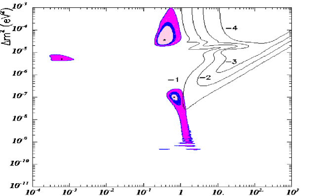
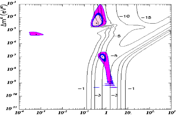
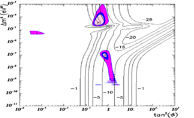
Figure 6: Likelihood ratio $\ln(R)$ relative to the SMA-MSW hypothesis, as function of $\tan^{2}\vartheta$ and $\Delta m^{2}$/eV² for $\tau=1.4$ (top), $\tau=1.7$ (middle) and $\tau=2$ (bottom) together with the 90, 95 and 99% CL contours for the different solutions to the solar neutrino problem from Ref. [10]. All figures for $E_{\rm b}=1.5\times 10^{53}$ erg and $\langle E_{\bar{\nu}_{\rm e}}\rangle=12$ MeV.

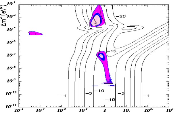
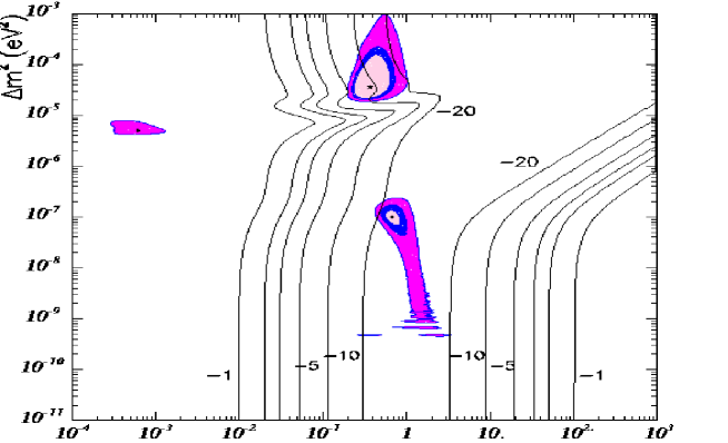
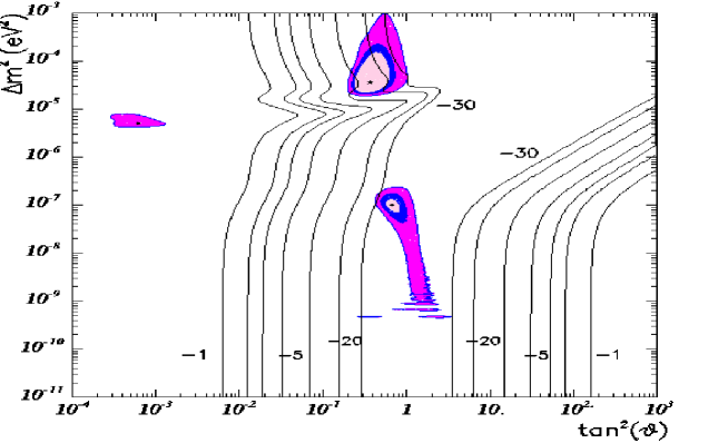
Figure 7: Likelihood ratio $\ln(R)$ relative to the SMA-MSW hypothesis, as function of $\tan^{2}\vartheta$ and $\Delta m^{2}$/eV² for $\tau=1.4$ (top), $\tau=1.7$ (middle) and $\tau=2$ (bottom) together with the 90, 95 and 99% CL contours for the different solutions to the solar neutrino problem from Ref. [10]. All figures for $E_{\rm b}=3\times 10^{53}$ erg and $\langle E_{\bar{\nu}_{\rm e}}\rangle=14$ MeV.

4 Kolmogorov-Smirnov test

We use the one-dimensional Kolmogorov-Smirnov (KS) test as described e.g. in Ref. [23] to estimate the probability that the observed data points $E_{i}$ agree with the spectral shape predicted by a given distribution $n_{\bar{\nu}_{e}}(E)$. The one-dimensional form of the KS test we apply has the disadvantage of being not sensitive to $E_{\rm b}$ viz. the amplitude of the neutrino signal. This disadvantage is however compensated by its property to be distribution-free that makes the one-dimensional KS test attractive. In Fig. 8, we show the probability that the signal observed in the two detectors is consistent with the SMA-MSW hypothesis, as function of $\langle E_{\bar{\nu}_{\rm e}}\rangle$. Performing this test for the two experiments separately, we find a small region of overlap at $\langle E_{\bar{\nu}_{\rm e}}\rangle\sim 11$ MeV where this hypothesis has a probability of more than 10% in both experiments. The combined data set has a probability higher than 10% in the broad range $\langle E_{\bar{\nu}_{\rm e}}\rangle=9~{}$MeV – 14 MeV, with a maximal probability of 46%. Since the maximum occurs at the same energies as the best-fit values found in the maximum-likelihood analysis, we conclude that the essential information is contained in the form of the spectra, not in the absolute number of events.

In Fig. 9, we show the same test for the LMA-MSW hypothesis. Its probability as function of $\langle E_{\bar{\nu}_{\rm e}}\rangle$ has the same shape as in the case of SMA-MSW but is shifted to lower energies by 0.7 MeV ($\tau=1.4$), 1.7 MeV ($\tau=1.7$) and 2.8 MeV ($\tau=2$), respectively. Consequently, an exclusion of the LMA-MSW solution because of its preference of low $\langle E_{\bar{\nu}_{\rm e}}\rangle$ requires a correspondingly precise knowledge of the average neutrino energies emitted by the SN. The maximum of the probability as function of $\langle E_{\bar{\nu}_{\rm e}}\rangle$ increases from 50% ($\tau=1.4$) to 65% ($\tau=1.7$) and 80% ($\tau=2$). Moreover, we find that the LMA-MSW hypothesis is consistent with the data at the 5% ($\tau=1.4$), 2% level ($\tau=1.7$) and 1% level ($\tau=2$) for $\langle E_{\bar{\nu}_{\rm e}}\rangle=14$ MeV, while the compatibility increases to 25% ($\tau=1.4$), 16% level ($\tau=1.7$) and 5% level ($\tau=2$) at the lower end of predicted neutrino energies, $\langle E_{\bar{\nu}_{\rm e}}\rangle=12$ MeV.

Finally, we present in Fig. 10 the results of the KS test for VO. Now the maxima of the probability as function of $\langle E_{\bar{\nu}_{\rm e}}\rangle$ compared to the SMA-MSW solution are shifted by 2.2 MeV ($\tau=1.4$), 3.7 MeV ($\tau=1.7$) and 5 MeV ($\tau=2$), respectively. The maximum of the probability increases from 59% ($\tau=1.4$) to 68% ($\tau=1.7$) and 70% ($\tau=2$). Thus the most probable value of $\langle E_{\bar{\nu}_{\rm e}}\rangle$ for $\tau=2$ is reduced by a factor two compared to SMA-MSW and also the cases $\tau=1.7$ and $\tau=1.4$ are highly incompatible with the range of neutrino temperatures predicted by simulations. On the other hand, VO together with rather low neutrino temperatures, $\langle E_{\bar{\nu}_{\rm e}}\rangle\approx 12$ MeV and $\tau=1.4$ are at the $2\sigma$ level compatible with the spectral shape of SN 1987A signal.

Figure 8: Probability $p$ as function of $\langle E_{\bar{\nu}_{\rm e}}\rangle$ given by the KS test that the observed data by Kam, IMB and the combined data set are consistent with the SMA-MSW oscillation hypothesis.

Figure 9: Probability $p$ as function of $\langle E_{\bar{\nu}_{\rm e}}\rangle$ given by the KS test that the combined data set is consistent with the LMA-MSW oscillation hypothesis for $\tau=1.4$, $\tau=1.7$ and $\tau=2$.

Figure 10: Probability $p$ as function of $\langle E_{\bar{\nu}_{\rm e}}\rangle$ given by the KS test that the combined data set is consistent with the VO hypothesis for $\tau=1.4$, $\tau=1.7$ and $\tau=2$.

5 Discussion and Conclusions

Recently, several papers discuss the influence of neutrino oscillations on the signal of SN 1987A. Reference [21] stresses that matter effects in the Earth partially regenerate the $\bar{\nu}_{e}$ flux in the case of LMA-MSW oscillations. This effect can be clearly seen in the plots of $R$ in the $\Delta m^{2}$-$\tan^{2}\vartheta$ plane, Figs. 6-7, where the likelihood of the LMA-MSW solution increases for $\Delta m^{2}\sim 10^{-5}$ eV². Furthermore, Ref. [21] finds that the KamII and IMB data sets become more compatible to each other for LMA-MSW oscillations because of the different Earth matter effects seen in the two detectors. The general tendency of their findings agrees with ours although there are some differences in the details. A possible explanation for the differences is the different approach used: Ref. [21] binned the IMB data into two bins while we used a continuous likelihood-function together with an experimental energy resolution function. Reference [24] concentrates on the question if an inverted mass hierarchy $m_{\nu_{3}}<m_{\nu_{1}}<m_{\nu_{2}}$ with $\Delta m^{2}_{12}=\Delta m^{2}_{\odot}$ and $\Delta m^{2}_{23}=\Delta m^{2}_{\rm atm}$ can be excluded by the SN1987 signal. They conclude that the SN 1987A signal disfavours this scheme unless $|U_{13}|^{2}\mathrel{\mathop{\kern 0.0pt\hbox to0.0pt{\raise 0.86108pt\hbox{$<$}\hss}}\lower 3.87495pt\hbox{\kern-1.90002pt$\sim$}}$ a few $10^{-4}$. Finally, the authors of Ref. [25] consider the compatibility of the LSND hint for $\bar{\nu}_{\mu}\leftrightarrow\bar{\nu}_{e}$ oscillations with the SN 1987A signal and find that the LSND result is disfavoured.

In this work, we have put the main emphasis on scrutinizing whether or not and to what extent large mixing oscillation solutions to the solar neutrino problem are really excluded by the SN 1987A signal. Our main result is that the LMA-MSW solution is not in conflict with the current understanding of supernova physics. In contrast, the VO and the LOW solutions to the solar neutrino problem can be excluded at the $4\sigma$ level, for most of the range of SN parameters found in simulations. Only a marginal region with low values of $\langle E_{\bar{\nu}_{\rm e}}\rangle$, $\langle E_{\bar{\nu}_{\mu,\tau}}\rangle$ and $E_{\rm b}$ is left over, in which these oscillation solutions can be reconciled with the neutrino signal of SN 1987A. If either of the large mixing solutions will be finally established by future solar neutrino experiments, the neutrino signal of SN 1987A will allow one to restrict severely the possible range of the neutrino energies and the released binding energy in SN explosions.

- [1] K. Hirata et al. [KAMIOKANDE-II Collaboration], “Observation of a neutrino burst from the supernova SN1987A,” Phys. Rev. Lett. 58, 1490 (1987); R.M. Bionta et al., “Observation of a neutrino burst in coincidence with supernova SN1987A in the Large Magellanic Cloud,” Phys. Rev. Lett. 58, 1494 (1987).
- [2] J. Arafune, M. Fukugita, T. Yanagida and M. Yoshimura, “Neutrino mass and mixing constrained from the LMC supernova burst,” Phys. Lett. B194, 477 (1987) and “Neutrino burst from SN1987A and the Solar neutrino puzzle,” Phys. Rev. Lett. 59, 1864 (1987); T.P. Walker and D.N. Schramm, “Resonant neutrino oscillations and the neutrino signature of supernovae,” Phys. Lett. B195, 331 (1987); D. Nötzold, “MSW effect analysis for SN1987A sets severe restrictions on neutrino masses and mixing angles,” Phys. Lett. B196, 315 (1987); H. Minakata, H. Nunokawa, K. Shiraishi and H. Suzuki, “Neutrinos from supernova explosion and the Mikheev-Smirnov-Wolfenstein effect,” Mod. Phys. Lett. A2, 827 (1987); H. Minakata and H. Nunokawa, “Neutrino flavor conversion in supernova SN1987A,” Phys. Rev. D38, 3605 (1988); T.K. Kuo and J. Pantaleone, ’‘Supernova neutrinos and their oscillations,” Phys. Rev. D37, 298 (1988); T.J. Loredo and D.Q. Lamb, “Neutrino from SN1987A: Implications for cooling of the nascent neutron star and the mass of the electron anti-neutrino,” Ann. N. Y. Acad. Sci. 571, 601 (1989).
- [3] A.Y. Smirnov, D.N. Spergel and J.N. Bahcall, “Is large lepton mixing excluded?,” Phys. Rev. D49, 1389 (1994) [hep-ph/9305204].
- [4] B. Jegerlehner, F. Neubig and G. Raffelt, “Neutrino oscillations and the supernova SN1987A signal,” Phys. Rev. D54, 1194 (1996) [astro-ph/9601111].
- [5] A. Burrows, “Supernova neutrinos,” Astrophys. J. 334, 891 (1988).
- [6] P.M. Givanoni, D.C. Ellison and S.W. Bruenn, “Neutrino transport during the core bounce phase of a type II supernova explosion,” Astrophys. J. 342, 416 (1989); H.-T. Janka and W. Hillebrandt, “Neutrino emission from type II supernovae: an analysis of the spectra,” Astron. Astrophys. 224, 49 (1989).
- [7] H.-T. Janka, in Proc. Frontier Objects in Astrophysics and Particle Physics, Vulcano 1992, eds. F. Giovaelli and G. Mannocchi.
- [8] H. Suzuki, in Frontiers of Neutrino Astrophsyics, ed. Y. Suzuki and K. Nakamura (Tokyo: Universal Academy 1993); S. Hannestadt and G. Raffelt, “Supernova Neutrino Opacity from Nucleon-Nucleon Bremsstrahlung and Related Processes,” Astrophys. J. 507, 339 (1998) [astro-ph/9711132]; A. Burrows, in SN1987A: Ten Years Later, ed. M.M. Phillips and N.B. Suntzeff, in press (2000).
- [9] A. Burrows, T. Young, P. Pinto, R. Eastman and T. Thompson, “Supernova neutrinos and a new algorithm for neutrino transport,” Astrophys. J. 539, 865 (2000) [astro-ph/9905132].
- [10] M.C. Gonzalez-Garcia, M. Maltoni, C. Peña-Garay and J.W.F. Valle, “Global three-neutrino oscillation analysis of neutrino data,” hep-ph/0009350 (Phys. Rev. D, in press); M.C. Gonzalez-Garcia and C. Peña-Garay, “Four-neutrino oscillations at SNO,” hep-ph/0011245.
- [11] Y. Fukuda et al. [Super-Kamiokande Collaboration], “Evidence for oscillation of atmospheric neutrinos,” Phys. Rev. Lett. 81, 1562 (1998) [hep-ex/9807003]; “Measurement of the flux and zenith-angle distribution of upward through-going muons by Super-Kamiokande,” ibid. 82, 2644 (1999) [hep-ex/9812014].
- [12] V. Barger, S. Pakvasa, T.J. Weiler and K. Whisnant, “Bi-maximal mixing of three neutrinos,” Phys. Lett. B437, 107 (1998) [hep-ph/9806387].
- [13] See, for example, S. Davidson and S.F. King, “Bi-maximal neutrino mixing in the MSSM with a single right-handed neutrino,” Phys. Lett. B445, 191 (1998) [hep-ph/9808296]; S.F. King and M. Oliveira, “Neutrino masses and mixing angles in a realistic string-inspired model,” hep-ph/0009287; A. de Gouvêa and J.W.F. Valle, “Minimalistic neutrino mass model,” hep-ph/0010299; P.H. Chankowski, A. Ioannisian, S. Pokorski and J.W.F. Valle, “Neutrino unification,” hep-ph/0011150.
- [14] J.C. Romão, M.A. Diaz, M. Hirsch, W. Porod and J.W.F. Valle, “A supersymmetric solution to the solar and atmospheric neutrino problems,” Phys. Rev. D61, 071703 (2000) [hep-ph/9907499]; M. Hirsch, M.A. Diaz, W. Porod, J.C. Romão and J.W.F. Valle, “Neutrino masses and mixings from supersymmetry with bilinear R-parity violation: A theory for solar and atmospheric neutrino oscillations,” Phys. Rev. D62, 113008 (2000) [hep-ph/0004115].
- [15] A. de Gouvêa, A. Friedland and H. Murayama, “The dark side of the solar neutrino parameter space,” Phys. Lett. B490, 125 (2000) [hep-ph/0002064]; M.C. Gonzalez-Garcia and C. Peña-Garay, “On the size of the dark side of the solar neutrino parameter space,” Phys. Rev. D62, 031301 (2000) [hep-ph/0002186]. G.L. Fogli, E. Lisi, D. Montanino and A. Palazzo, “Quasi-vacuum solar neutrino oscillations,” Phys. Rev. D62, 113004 (2000) [hep-ph/0005261].
- [16] G. Raffelt and J. Silk, “Can a mass inversion save solar neutrino oscillations from the Los Alamos neutrino?,” Phys. Lett. B366, 429 (1996) [hep-ph/9502306].
- [17] G.G. Raffelt, Stars as Laboratories for Fundamental Physics, Chicago University Press, 1996; S. Bludman, D.H. Feng, T. Gaisser and S. Pittel (eds.), “The Physics of supernovae”, Phys. Rept. 256, 1 (1995); A. Burrows and T. Young, Phys. Rept. 333-334, 63 (2000).
- [18] H.-T. Janka, “When do supernova neutrinos of different flavors have similar luminosities but different spectra?,” Astropart. Phys. 3, 377 (1995) [astro-ph/9503068].
- [19] M. Apollonio et al., “Limits on neutrino oscillations from the CHOOZ experiment,” Phys. Lett. B466, 415 (1999) [hep-ex/9907037]; F. Boehm et al., hep-ex/9912050
- [20] T.K. Kuo and J. Pantaleone, “Nonadiabatic neutrino oscillations in matter,” Phys. Rev. D39, 1930 (1989).
- [21] C. Lunardini and A.Y. Smirnov, “Neutrinos from SN1987A, Earth matter effects and the LMA solution of the solar neutrino problem,” hep-ph/0009356; see also A.Y. Smirnov, in V.A. Kozyarivsky (ed.), Proceedings of the 20th International Cosmic Ray Conference, Moscow 1987, Nauka 1987.
- [22] A. Gelman, J.B. Carlin, H.S. Stern and D.B. Rubin, Bayesian Data Analysis, Chapman and Hill, London 1995.
- [23] W.H. Press, S.A. Teukolsky, W.T. Vetterling and B.P. Flannery, Numerical Recipes, Cambridge University Press 1986.
- [24] H. Minakata and H. Nunokawa, “Inverted hierarchy of neutrino masses disfavored by supernova 1987A,” hep-ph/0010240.
- [25] H. Murayama and T. Yanagida, “LSND, SN1987A, and CPT violation,” hep-ph/0010178.