Simple solutions of fireball hydrodynamics
for self-similar elliptic flows

Abstract

Simple, self-similar, elliptic solutions of non-relativistic fireball hydrodynamics are presented, generalizing earlier results for spherically symmetric fireballs with Hubble flows and homogeneous temperature profiles. The transition from one dimensional to three dimensional expansions is investigated in an efficient manner.

¹ Bogolyubov Institute for Theoretical Physics, Kiev 03143, Metrologicheskaya 14b,Ukraine
² MTA KFKI RMKI, H - 1525 Budapest 114, POB 49, Hungary
³ Faculty of Science, Eötvös University,Budapest H-1117, Pázmány P. s. 1/A, Hungary

Introduction. Recently, a lot of experimental and theoretical efforts have gone into the exploration of hydrodynamical behavior of strongly interacting hadronic matter in non-relativistic as well as in relativistic heavy ion collisions, see e.g. [1] - [2]. Due to the non-linear nature of hydrodynamics, exact hydro solutions are rarely found. Those events, sometimes, even stimulate an essential progress in physics. One of the most impressive historical example is Landau’s one-dimensional analytical solution (1953) for relativistic hydrodynamics [3] that gave rise to a new (hydrodynamical) approach in high energy physics. The boost-invariant Bjorken solution [4], found more than 20 years later, is frequently utilized as the basis for estimations of initial energy densities in ultra-relativistic nucleus-nucleus collisions.

The obvious success of hydrodynamic approach to high energy nuclear collisions raise interest in an analogous description of non-relativistic collisions, too. The first exact non-relativistic hydrodynamic solution describing expanding fireballs was found in 1979 [5]. It has been generalized for fireballs with Gaussian density and homogeneous temperature profiles [6] as well as for fireballs with arbitrary initial temperature profiles [7] and corresponding, non-Gaussian density profiles. All of these solutions have spherical symmetry and a Hubble-type linear radial flow. However, a non-central collision has none of the mentioned symmetries. The purpose of this Letter is to present and analyze hydro solutions for such cases. The results presented in this paper may be utilized to access the time-evolution of the hydrodynamically behaving, strongly interacting matter as probed by non-central non-relativistic heavy ion collisions [8, 9]. As the hydro equations have no intrinsic scale, the results are rather general in nature and can be applied to any physical phenomena where the non-relativistic hydrodynamical description is valid.

Generalization of spherical solutions to elliptic flows. Consider an ideal fluid, where viscosity and heat conductivity are negligible, described by the local conservation of matter (continuity equation), the local conservation of energy (energy equation) and the local conservation of momentum (Euler equation):

$${\frac{\partial n}{\partial t}}+{\rm\bf\nabla}({\rm\bf v}n) = 0,$$ (1)

$${\frac{\partial\varepsilon}{\partial t}}+{\rm\bf\nabla}({\rm\bf v}\varepsilon) = -P{\rm\bf\nabla}{\rm\bf v},$$ (2)

$$mn({\frac{\partial}{\partial t}}+{\rm\bf v}{\rm\bf\nabla}){\rm\bf v} = -{{\rm\bf\nabla}P},$$ (3)

where $m$ is the mass of a single particle and $n=n(t,{\rm\bf r}),$ ${\rm\bf v}={\rm\bf v}(t,{\rm\bf r}),$ $P=P(t,{\rm\bf r})$ and $\varepsilon=\varepsilon(t,{\rm\bf r})$ are the local density of the particle number, the velocity, the pressure and the energy density fields, respectively. To complete the set of equations we need to fix the equations of state. For reasons of simplicity we have chosen the equations of state to be those of an ideal, structureless Boltzmann gas:

$$\varepsilon(t,{\rm\bf r}) = {\frac{3}{2}}P(t,{\rm\bf r}),$$ (4)

$$P(t,{\rm\bf r}) = n(t,{\rm\bf r})T(t,{\rm\bf r}).$$ (5)

The solutions that are presented in the subsequent parts cannot be trivially generalized to any arbitrary equations of state. Nevertheless, they provide a transparent insight into the collective physical processes in a non-central heavy ion collision.

In the following, we utilize the above ideal gas equation of state and rewrite the hydrodynamical equations in terms of the three functions $n$,${\rm\bf v}$ and $T$.

In ref. [6, 7], special classes of exact analytic solutions of fireball hydrodynamics were found assuming spherical symmetry and self-similar Hubble flows. In ref. [6] a homogeneous temperature profile was assumed, while the general solution for arbitrary, inhomogeneous initial temperature profiles was found in ref. [7]. In these articles, the concept of self-similarity meant that there is a typical length-scale of the expanding system $R=R(t)$ so that all space-time functions in the hydro equations are of the form $F=G(t)H(s)$ where $s=r^{2}/R^{2}$ is the so-called (dimensionless) scaling variable.

Let us go beyond spherical symmetry and consider three typical lengths of the expanding system: $X,Y$ and $Z$, all functions of time only. Let us rotate our frame of reference to the major axis of the ellipsoidal expansion, and leave to future applications to relate these major axes to the laboratory frame. Consequently, let us introduce three scaling variables $x=r_{x}^{2}/X^{2}$, $y=r_{y}^{2}/Y^{2}$ and $z=r_{z}^{2}/Z^{2}$ and assume that all space-time functions are of the form of $F=G(t)H(x)K(y)L(z)$. Using this ansatz we find that the continuity equation is satisfied regardless of the density profile if the velocity field is a Hubble-flow field in each principal direction:

$$v_{x}(t,{\rm\bf r}) = {\frac{\dot{X}(t)}{X(t)}}r_{x},$$

$$v_{y}(t,{\rm\bf r}) = {\frac{\dot{Y}(t)}{Y(t)}}r_{y},$$

$$v_{z}(t,{\rm\bf r}) = {\frac{\dot{Z}(t)}{Z(t)}}r_{z}.$$ (6)

Although our sole assumption concerning the temperature was the ansatz form already mentioned, we found that the Euler equation requires the temperature to be homogeneous, independent of the coordinate variables: $T=T(t)$. The energy equation is only satisfied if

$$T(t)=T_{0}\left({\frac{\displaystyle\phantom{|}V_{0}}{\displaystyle\phantom{|}V(t)}}\right)^{2/3},$$ (7)

where $V(t)=X(t)Y(t)Z(t)$ is the typical volume of the expanding system, while $V_{0}=V(t_{0})$ and $T_{0}=T(t_{0})$ are the initial temperature and volume. The homogeneity of the temperature and the Euler equation implied that the density profile is a product of three Gaussians, with different, time dependent radius parameters:

$$n(t,{\rm\bf r})=n_{0}{\frac{\displaystyle\phantom{|}V_{0}}{\displaystyle\phantom{|}V(t)}}\exp\left(-{\frac{\displaystyle\phantom{|}r_{x}^{2}}{\displaystyle\phantom{|}2X(t)^{2}}}-{\frac{\displaystyle\phantom{|}r_{y}^{2}}{\displaystyle\phantom{|}2Y(t)^{2}}}-{\frac{\displaystyle\phantom{|}r_{z}^{2}}{\displaystyle\phantom{|}2Z(t)^{2}}}\right),$$ (8)

where $n_{0}=n(0,{\rm\bf 0})$ can be expressed by the total number of particles ($N$) as

$$n_{0}=\frac{1}{(2\pi)^{3/2}}\frac{N}{V_{0}}.$$ (9)

The time evolution of the scales are determined - through the Euler equation - by the equations

$$\ddot{X}X=\ddot{Y}Y=\ddot{Z}Z=\frac{T_{0}}{m}\left({\frac{\displaystyle\phantom{|}V_{0}}{\displaystyle\phantom{|}V}}\right)^{2/3}.$$ (10)

This system of non-linear, second-order ordinary differential equations has a unique solution for the scale-functions if the initial parameters $X_{0}$, $Y_{0}$, $Z_{0}$ and $\dot{X}_{0}$, $\dot{Y}_{0}$, $\dot{Z}_{0}$ are given. Although this solution has not yet been found in an explicite, analytic form, some of its properties are determined in the subsequent parts.

Properties of the elliptic solutions. Global conservation laws reflect, in general, boundary conditions for solutions, or their behavior at asymptotically large distances. Because of reflection symmetry of densities and velocities, the conservation of momentum, ${\rm\bf P}=0$, is satisfied automatically and gives no non-trivial first integral. On the other hand, the asymptotically fast decreasing of the densities give us the possibility of using total energy conservation as

$$\frac{\partial}{\partial t}\int d^{3}r(\varepsilon+\frac{nmv^{2}}{2})=0$$ (11)

to find the first integral of the system of equations (1) - (3). Substitute (6), (8) into (11), we get:

$$\stackrel{{\scriptstyle.}}{{X}}^{2}+\stackrel{{\scriptstyle.}}{{Y}}^{2}+\stackrel{{\scriptstyle.}}{{Z}}^{2}+3\frac{T_{0}}{m}\left({\frac{\displaystyle\phantom{|}V_{0}}{\displaystyle\phantom{|}V}}\right)^{2/3}=A\,=const.$$ (12)

Using (10) one can rewrite (12) in the form

$$\frac{1}{2}\frac{\partial^{2}}{\partial t^{2}}(X^{2}+Y^{2}+Z^{2})=A,$$ (13)

and find finally

$$R^{2}(t)=X^{2}(t)+Y^{2}(t)+Z^{2}(t)\,=\,A(t-t_{0})^{2}+B(t-t_{0})+C,$$ (14)

where

$$A = \stackrel{{\scriptstyle.}}{{X}}_{0}^{2}+\stackrel{{\scriptstyle.}}{{Y}}_{0}^{2}+\stackrel{{\scriptstyle.}}{{Z}}_{0}^{2}+3\frac{T_{0}}{m},$$

$$B = 2(X_{0}\stackrel{{\scriptstyle.}}{{X}}_{0}+Y_{0}\stackrel{{\scriptstyle.}}{{Y}}_{0}+Z_{0}\stackrel{{\scriptstyle.}}{{Z}}_{0}),$$

$$C = X_{0}^{2}+Y_{0}^{2}+Z_{0}^{2}.$$ (15)

The simple equation (14) express the general property of elliptic hydrodynamic flows. The value of radius-vector evolves in time similar to a ”particle” with coordinates $(X,Y,Z)$ that moves in a non-central, repulsive potential according to eqs. (10). In particular, one may introduce the canonical coordinates $(X,Y,Z)$ and the canonical momenta as $(P_{x},P_{y},P_{z})=m(\dot{X},\dot{Y},\dot{Z})$ and the Hamiltonian $H$ as a rewritten form of eq.  (12):

$$H=\frac{1}{2m}\left(P_{x}^{2}+P_{y}^{2}+P_{z}^{2}\right)+\frac{3}{2}T_{0}\left(\frac{X_{0}Y_{0}Z_{0}}{XYZ}\right)^{2/3}$$ (16)

The Hamiltonian equations of motion can be written in terms of Poisson brackets as $\dot{X}=\left\{X,H\right\}$, … , $\dot{P_{x}}=\left\{P_{x},H\right\}$, … . The Lagrangian form of these equations is given by eqs. (10). Due to the repulsive nature of the potential, the coordinates $(X,Y,Z)$ diverge to infinity for large times. As the potential vanishes for large values of the coordinates, the canonical momenta tend to constant values for asymptotically large times.

Eq. (12) expresses the conservation of whole energy (kinetic and potential) of the ”particle”, corresponding to $H(X,...,P_{x},...)=E=const$. The resulting eq. (14) has also great importance for the analysis of approximate analytical solutions. It is worth mentioning another interesting relation that one can get from (12) for asymptotic times $t_{as},$ when $V(t_{as})\gg V_{0}$:

$$\frac{m}{2}\left(\stackrel{{\scriptstyle.}}{{X}}_{as}^{2}+\stackrel{{\scriptstyle.}}{{Y}}_{as}^{2}+\stackrel{{\scriptstyle.}}{{Z}}_{as}^{2}\right)=\frac{m}{2}\left(\stackrel{{\scriptstyle.}}{{X}}_{0}^{2}+\stackrel{{\scriptstyle.}}{{Y}}_{0}^{2}+\stackrel{{\scriptstyle.}}{{Z}}_{0}^{2}\right)+\frac{3}{2}T_{0}.$$ (17)

This relation expresses the equality of the initial flow and internal energy with the asymptotic energy which is present in the form of flow.

Although eqs. (10) are easy to handle with presently available numerical packages, we note that a further simplification of these equations to a non-linear first order differential equation of one variable is possible, if an additional cylindrical symmetry is assumed, corresponding to $X(t)=Y(t)$. One may introduce the angular variable $\phi=\arccos(Z/R)$ so that

$$X(t) = Y(t)\,=\,\frac{1}{\sqrt{2}}R(t)\sin\phi(t)$$ (18)

$$Z(t) = R(t)\cos\phi(t).$$ (19)

The time evolution of $\phi(t)$ is determined by the following first order equation:

$$\dot{\phi}^{2}=\frac{1}{R^{2}(t)}\left[\frac{E}{m}-\dot{R}^{2}(t)-\frac{3}{2}\frac{T_{0}}{m}\frac{(X_{0}^{2}Z_{0})^{2/3}}{R^{2}(t)}\frac{1}{(\sin\phi)^{4/3}\,(\cos\phi)^{2/3}}\right]$$ (20)

where $R(t)$ is given explicitly by eq. (14).

Figs. 1-4 indicate the results of numerical solutions of eqs. (10). Using Landau-type initial conditions, one confirms that even the full three-dimensional solution results in a small amount of transverse flow generation, while for more general initial conditions, significant amount of transverse flow can be generated. Transverse flow is stronger if the initial conditions are closer to spherical symmetry or, if the fraction of the initial thermal energy is increased as compared to the initial kinetic energy. For more details, see the figure captions.

In the last part an approximate, analytic solution is presented that corresponds to Landau-like, one dimensional expansions.

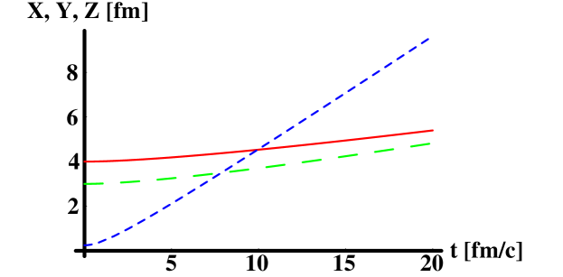
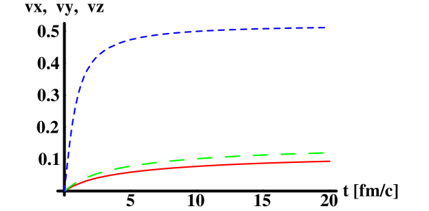
Figure 1: Top panel shows the time dependence of the major axis of the ellipsoidal (Gaussian) density profile, eq. (8), while the bottom panel indicates the velocity of expansion at the rms radii, $r_{x}=X(t)$, $r_{y}=Y(t)$ and $r_{z}=Z(t)$, for three dimensional, self-similar elliptic flows. Solid lines stand for $X(t)$ and $v_{x}(t)$, dashed lines for $Y(t)$ and $v_{y}(t)$, short-dashed lines for $Z(t)$ and $v_{z}(t)$. The initial conditions are: $X_{0}=4$ fm, $Y_{0}=3$ fm, $Z_{0}=1/4$ fm, the initial velocities are all vanishing, $T_{0}/m=0.1$ . Due to the Landau-like initial condition (strong initial compression in the $z$ direction), the flow is almost one dimensional, only small amount of transverse flow is generated in this case.

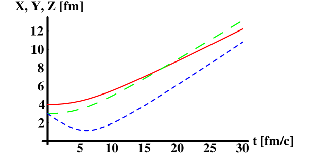
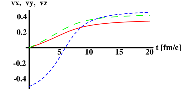
Figure 2: Same as Fig. 1, but for a more spherical initial profile with an initial inwards flow in the $z$ direction. The initial conditions are: $X_{0}=4$ fm, $Y_{0}=3$ fm, $Z_{0}=3$ fm, the initial velocities are $\dot{X}_{0}=0$, $\dot{Y}_{0}=0$, $\dot{Z}_{0}=-0.5$, while $T_{0}/m=0.1$ . Due to the deviation from the Landau-like initial condition, the final flow is almost spherically symmetric, three dimensional, and a large amount of transverse flow is generated in this case.

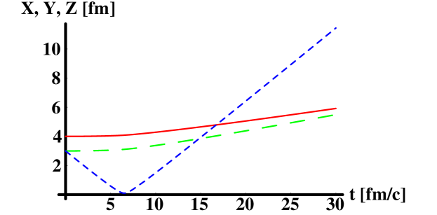
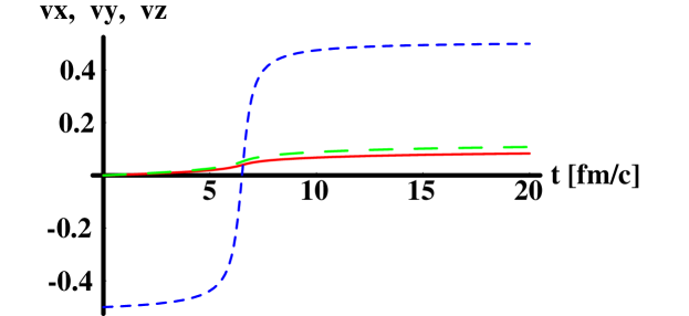
Figure 3: Same as Fig. 3, but for $T_{0}/m=0.01$. This corresponds to increasing the initial kinetic energy as compared to the internal (thermalized) energy, and in this case the flow becomes approximately one dimensional again. The initial conditions are: $X_{0}=4$ fm, $Y_{0}=3$ fm, $Z_{0}=3$ fm, the initial velocities are $\dot{X}_{0}=0$, $\dot{Y}_{0}=0$, $\dot{Z}_{0}=-0.5$, while $T_{0}/m=0.01$ .

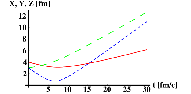
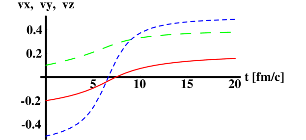
Figure 4: A more general initial condition may result even in a dominantly two-dimensional expansion. The initial conditions are: $X_{0}=4$ fm, $Y_{0}=3$ fm, $Z(0)=3$ fm, the initial velocities are $\dot{X}_{0}=-0.2$, $\dot{Y}_{0}=0.1$, $\dot{Z}_{0}=-0.5$, while $T_{0}/m=0.05$ .

Approximate one-dimensional solutions. Hydrodynamical evolution, which is described by Eqs. (1) - (3), starts from some initial conditions. Consider Landau-type initial conditions (longitudinally compressed ”ellipsoid”), corresponding to the real situation in non-relativistic heavy ion collisions:

$$\stackrel{{\scriptstyle.}}{{X}}_{0}=\stackrel{{\scriptstyle.}}{{Y}}_{0}=0,\,Z_{0}\ll X_{0},\,Z_{0}\ll Y_{0},$$ (21)

and in general case $\stackrel{{\scriptstyle.}}{{Z}}_{0}\neq 0$. The last reflects the situation when a system is (locally) thermalized before, after or at the moment of full nuclear stopping and transverse expansion starts to develop only after the local thermalization. Then in some time interval $t_{0}\leq t\leq\widetilde{t}$ the hydro evolution is quasi - one - dimensional:

$$\frac{X(t)}{X_{0}}\approx 1,\,\frac{Y(t)}{Y_{0}}\approx 1,\,$$ (22)

and the equation of motion for $Z(t)$ takes the following form

$$\ddot{Z}Z=\frac{T_{0}}{m}\left({\frac{\displaystyle\phantom{|}Z_{0}}{\displaystyle\phantom{|}Z}}\right)^{2/3}.$$ (23)

This equation has an exact analytic solution,

$$Z^{2}(t)=(\widetilde{Z}_{0}^{2/3}+(a_{+}+a_{-})^{2})^{3},$$ (24)

where

$$a_{\pm} = \left(\frac{1}{2}\widetilde{Z}(t)\pm\left(\widetilde{Z}_{0}^{2}+\frac{1}{4}\widetilde{Z}^{2}(t)\right)^{1/2}\right)^{1/3},$$

$$\widetilde{Z}(t) = \sqrt{3u^{2}}(t-\widetilde{t}_{0}),\,u^{2}=\frac{1}{3}\left(\stackrel{{\scriptstyle.}}{{Z}}_{0}^{2}+3\frac{T_{0}}{m}\right),$$

$$\widetilde{Z}_{0} = \left(\frac{T_{0}}{mu^{2}}\right)^{3/2}Z_{0},\,\widetilde{t}_{0}=t_{0}-\frac{Z_{0}\stackrel{{\scriptstyle.}}{{Z}}_{0}}{3u^{4}}(u^{2}+\frac{T_{0}}{m}).$$ (25)

Here $\widetilde{t}_{0}$ is the turning point for $Z^{2}(t)$ if $\stackrel{{\scriptstyle.}}{{Z}}_{0}<0$. Using (14) we obtain that the conditions for validity of the solution (22), (24) are satisfied within some time interval $t_{0}\leq t\leq\widetilde{t}$ if

$$\left|\frac{A(t-t_{0})^{2}+B(t-t_{0})+Z_{0}^{2}-Z^{2}(t)}{X_{0}^{2}+Y_{0}^{2}}\right|\ll 1.$$ (26)

The hydrodynamical evolution described by the equations (1) - (3) cannot be continued infinitely in time, because the general criteria of applicability of hydrodynamical description are violated: the mean free path $l\propto 1/(\sigma n)$ has to be (much) smaller than the typical length scales of the system, for example the effective geometrical sizes or hydrodynamic lengths. Due to the hydrodynamical expansion the density (8) will decrease with time reaching some critical value that can be estimated utilizing Landau’s criterium, $T=m_{\pi},$ that determines a critical density when hydrodynamic evolution breaks up. Here, we will use a simplified version of this criterium and suppose the decoupling of hydrodynamical system when density in the center of the system reaches some critical value $n_{f}$ (typically, normal nuclear density). Then the time $t_{f\,}$, when the hydrodynamical evolution ends, can be estimated from the condition

$$n(t_{f},{\rm\bf 0})=n_{f},$$ (27)

If the hydrodynamical evolution stops before the condition (26) is violated, $t_{f\,}<\widetilde{t}$, then solutions (22) and (24) describing quasi-one-dimensional expansion give complete hydrodynamical evolution, too. Let us find the conditions for such a situation. Supposing quasi-one-dimensional expansion and using (8) and (22) we get

$$\frac{Z(t_{f})}{Z_{0}}=\frac{n_{0}}{n_{f}}.$$ (28)

Then using (24) we can find $t_{f}$. If for $t=t_{f}$ the inequality (26) is satisfied, then we can conclude that $t_{f\,}<\widetilde{t}$ and the one dimensional expansion is valid approximation until the freeze-out time.

It is useful to give simple analytical estimations of the initial hydrodynamic conditions that guarantee quasi-one-dimensional expansion of the nuclear matter. Let us suppose, for simplicity, that $\stackrel{{\scriptstyle.}}{{Z}}_{0}=0$ and hence $u^{2}=\frac{T_{0}}{m},$ $\widetilde{Z}_{0}=Z_{0}$, $\widetilde{t}_{0}=t_{0}$ in (24). Supposing that the upper time limit of quasi-one-dimensional expansion, $\widetilde{t},$ is large enough so that

$$\widetilde{Z}^{2}(\widetilde{t})\gg 4Z_{0}^{2},$$

we can rewrite Eq.(24) in the form:

$$Z^{2}(\widetilde{t})\approx\widetilde{Z}^{2}(\widetilde{t})-3(Z_{0}\widetilde{Z}^{2}(\widetilde{t}))^{2/3}.$$ (29)

After substitution (29) in (26) we obtain:

$$\frac{3\frac{T_{0}}{m}(\widetilde{t}-\widetilde{t}_{0})^{2}}{X_{0}^{2}+Y_{0}^{2}}\ll\frac{1}{3\sqrt{3}}\frac{\sqrt{X_{0}^{2}+Y_{0}^{2}}}{Z_{0}}.$$ (30)

It is easy to see from (30) that for large enough $\frac{X_{0}^{2}+Y_{0}^{2}}{Z_{0}^{2}}$ , quasi-one-dimensionality can hold till the longitudinal scale becomes comparable to transversal ones:

$$\frac{Z^{2}(\widetilde{t})}{X^{2}(\widetilde{t})+Y^{2}(\widetilde{t})}\approx\frac{\widetilde{Z}^{2}(\widetilde{t})}{X_{0}^{2}+Y_{0}^{2}}\approx\frac{Z^{2}(\widetilde{t})}{X_{0}^{2}+Y_{0}^{2}}\propto 1$$ (31)

It means that within time $t<$ $\widetilde{t}$ solution (22), (24) correctly describes the transformation of longitudinally compressed ”ellipsoid” to ”spheroid” form. Finally from (28) we get that $Z(t_{f})<Z(\widetilde{t})\propto\sqrt{X_{0}^{2}+Y_{0}^{2}}$ and consequently $t_{f}<\widetilde{t}$ if

$$\frac{n_{0}}{n_{f}}<\frac{\sqrt{X_{0}^{2}+Y_{0}^{2}}}{Z_{0}}$$ (32)

Under such initial conditions one can expect that whole stage of the hydrodynamical evolution can be correctly described by the approximate quasi-one-dimensional solution (22) and (24).

Summary and conclusions: In this Letter we considered the time evolution of fireball hydrodynamics describing an ideal gas, an elliptic initial density profile, a homogeneous temperature distribution and a Hubble-like flow distribution. For this case, the set of partial differential equations of non-relativistic hydrodynamics have been reduced to a set of ordinary, second order, non-linear differential equations, that can be solved efficiently by presently available numerical packages without the need of sophisticated programming. The initial conditions for these equations are associated with the initial elliptic sizes $X_{0}$, $Y_{0}$ and $Z_{0}$, that could be linked with the overlapping geometrical sizes of colliding nuclei in heavy ion collisions and with the dynamics of the compression process during interactions during the pre-thermal time evolution.

The general behavior of these hydrodynamical equations is determined analytically and related to the Hamiltonian motion of a particle in a repulsive, non-central potential. A first integral of motion has been found, corresponding to the conservation of energy in the Hamiltonian problem. It was utilized to obtain an approximate solution for quasi one-dimensional expansions and to determine the domain of applicability of this solution.

The importance of the results is given by recent experimental findings in high energy heavy ion reacions, where various elliptic flow patters are observed, see refs. [10, 11, 12, 13] for further details. In future studies, our results could be applied to gain insight into the interpretation of the above mentioned data and to describe nucleus-nucleus collisions with non-relativistic initial energies. Such conditions for a non-relativistic evolution may be reached in the mid-rapidity region near to the softest point of equation of state even in relativistic heavy ion collisions, if the pressure is not strong enough to build up a relativistic transverse flow. Due to the scale invariance of the hydrodynamical equations the solutions described here can also be utilized in other problems related to elliptic flows in non-spherical fireball hydrodynamics.

Acknowledgments: This research has been supported by a Bolyai Fellowship of the Hungarian Academy of Sciences and by the grants OTKA T024094, T026435, T029158, the US-Hungarian Joint Fund MAKA grant 652/1998, NWO - OTKA N025186, Hungarian - Ukrainian S& T grant 45014 (2M/125-199) and the grants FAPESP 98/2249-4 and 99/09113-3 of Sao Paolo, Brazil.

References

- [1] L. P. Csernai, Introduction to Relativistic Heavy Ion Collisions, John Wiley and Sons, 1994
- [2] D. H. Rischke, Nucl. Phys. A610 (1996) 88c
- [3] L. D. Landau, Izv. Akad. Nauk SSSR 17 (1953) 51; in “Collected papers of L. D. Landau” (ed. D. Ter-Haar, Pergamon, Oxford, 1965) p. 665 - 700
- [4] J. D. Bjorken, Phys. Rev. D27 (1983) 140
- [5] J. Bondorf, S. Garpman and J. Zimányi, Nucl. Phys. A296 (1978) 320 - 332
- [6] P. Csizmadia, T. Csörgő and B. Lukács, Phys. Lett. B443 (1998) 21-25
- [7] T. Csörgő, nucl-th/9809011
- [8] T. Csörgő, B. Lörstad and J. Zimányi, Phys. Lett. B338 (1994) 134-140
- [9] J. Helgesson, T. Csörgő, M. Asakawa and J. Zimányi, Phys. Rev. C56 (1997) 2626 - 2635
- [10] A. M. Poskanzer et al., Nucl. Phys. A 661 (1999) 341
- [11] K. H. Ackermann et al., nucl-ex/0009011
- [12] L. P. Csernai and D. Rohrich, Phys. Lett. B 458 (1999) 454
- [13] S. A. Voloshin and A. M. Poskanzer, Phys. Lett. B 474 (2000) 27