TPI-MINN-00/65

UMN-TH-1931

hep-ph/0012123

December 2000

The $b$–quark EDM in SUSY and CP–odd bottomonium formation

D. A. Demir${}^{{}^{1}}$ and M. B. Voloshin${}^{{}^{1,2}}$

${}^{{}^{1}}$ Theoretical Physics Institute, University of Minnesota, Minneapolis, MN 55455

${}^{{}^{2}}$ Institute of Theoretical and Experimental Physics, Moscow, 117259

Abstract

We compute the electric dipole moment (EDM) of the bottom quark in minimal supersymmetric model (SUSY) with explicit CP violation. We estimate its upper bound to be $10^{-20}~{}{\rm e-cm}$ where the dominant contribution comes from the charginos for most of the SUSY parameter space. We also find that chargino contribution is directly correlated with the branching fraction of the $B\rightarrow X_{s}\gamma$ decay. Furthermore, we analyze the formation of ${}^{1}\mbox{P}_{1}$ resonance of the $(\bar{b}b)$ system in $e^{+}e^{-}$ annihilation, and show that the CP–violating transition amplitude, induced solely by the $b$–quark EDM, is significantly larger than the CP–conserving ones. Therefore, observation of this CP–odd resonance in $e^{+}e^{-}$ annihilation will be a direct probe of the CP–violating phases in SUSY. In case experiment cannot establish the existence of such a CP–odd $(\bar{b}b)$ state, then either sparticle masses of all three generations will be pushed well above TeV, weakening the possibility of weak–scale SUSY, or the sparticle mass spectrum will be tuned so as to cancel different contributions to EDMs.

1 Introduction

In the minimal standard model (SM) of electroweak interactions both flavour violation and CP violation are encoded in the CKM matrix. In its supersymmetric (SUSY) extension, however, there appear new sources for these phenomena generated by the soft SUSY–breaking terms [1]. In an attempt to establish the strength and structure of the flavour and CP violation in SUSY it is necessary to confront it with the experimental data on flavour–changing and flavour–conserving processes. In this respect, the flavour–conserving phenomena such as the Higgs system [2] and the electric dipole moments (EDM) [3, 4, 5] of particles are useful tools in searching for new sources of CP violation in a way independent of the flavour violation.

The existing upper bounds on the neutron and electron EDMs [6] put stringent constraints on the sources of CP violation. Even if one solves the strong CP problem by a SUSY version [7] of the KSVZ axion model [8], the reamining electroweak contributions are to be still suppressed. For accomplishing this, there have been several suggestions which include ($i$) choosing [3] (or suppressing by a relaxation mechanism [9]) the SUSY CP phases $\stackrel{{\scriptstyle<}}{{\scriptscriptstyle\sim}}{\cal{O}}(10^{-3})$, or ($ii$) finding appropriate parameter domain where different contributions cancel [4], or ($iii$) making the first two generations of scalar fermions heavy enough [5] but keeping the soft masses of the third generation below ${\rm TeV}$. Though each scenario for suppressing the EDMs has its own virtues in terms of the implied SUSY parameter space, in what follows we will work in the framework of effective supersymmetry [10] where the scenario ($iii$) can be accomodated. However, the discussions below are general enough to be interpreted or extended in any of the scenarios listed above.

The effective SUSY scenario deals with a single generation of sfermions, and thus, the question of flavour–changing transitions is avoided. Then SUSY effects can show up through the Higgs bosons, Higgs and gauge fermions, and the third generation sfermions. In fact, it is these light sparticles that regenerate the electron and neutron EDMs by two–loop quantum effects [11, 12]. Moreover, it is clear that the third generation fermions can still have large EDMs as the one–loop SUSY contributions cannot be suppressed for them.

In Section 2 we will compute the bottom quark EDM in effective SUSY up to two–loop accuracy. We will see that the two–loop contributions are directly constrained by the electron and neutron EDMs which can exist only at two– and higher loop levels [12]. Concerning the one–loop effects, the chargino contribution to the bottom EDM will be shown to be fully constrained by the measured branching fraction [13] of the rare $b\rightarrow X_{s}\gamma$ decay. On the other hand, the gluino and neutralino contributions remain unconstrained; however, their contributions will be seen to hardly compete with that of the charginos.

Secion 3 is devoted to a detailed discussion of the possible signatures of a finite bottom quark EDM. In particular, we will discuss the formation of the ${}^{1}\mbox{P}_{1}$ bottomonium level in the $e^{+}e^{-}$ annihilation. It will be seen that the CP–violating process, generated by the bottom EDM, dominates over the CP–conserving ones. Therefore, possible detection of this CP–odd resonance can be a direct probe of the bottom EDM, or equivalently, the sources of CP–violation in SUSY.

Section 4 contains our concluding remarks.

2 The bottom quark EDM in SUSY

The dimension–five electric dipole operator

$${\cal{L}}_{EDM}={\cal{D}}_{b}\ \overline{b}(x)\ {\stackrel{{\scriptstyle\longleftrightarrow}}{{\partial_{\alpha}}}}\ \gamma_{5}\b{(}x)\ A^{\alpha}(x)$$ (1)

defines the EDM of the bottom quark at the natural mass scale of $Q\sim m_{b}$. Since ${\cal{D}}_{b}$ is obtained after integrating out all heavy degrees of freedom, it serves as a probe of the sources of CP violation at the weak scale $Q\sim M_{W}$. In the SM, ${\cal{D}}_{b}$ arises at three– and higher loop levels [15] whereas in SUSY there exist nonvanishing contributions already at the one–loop level [3]. In the SUSY parameter space under concern, the EDM of $b$–quark receives one–loop contributions from the exchange of gluinos (${\cal{D}}_{b}^{\tilde{g}}$), neutralinos (${\cal{D}}_{b}^{\chi^{0}}$) and charginos (${\cal{D}}_{b}^{\chi^{\pm}}$). Then, including also the two–loop contribution, the full expression for the bottom EDM reads symbolically as

$${{\cal{D}}_{b}} = {\cal{D}}_{b}^{\tilde{g}}\left[\tan\beta\sin\phi_{\mu},\sin\phi_{A_{b}}\right]+{\cal{D}}_{b}^{\chi^{0}}\left[\tan\beta\sin\phi_{\mu},\sin\phi_{A_{b}}\right]+{\cal{D}}_{b}^{\chi^{\pm}}\left[\tan\beta\sin\phi_{\mu},\sin\phi_{A_{t}}\right]$$ (2)

$$+ {\cal{D}}_{b}^{2-loop}\left[\tan\beta\sin\left(\phi_{\mu}+\phi_{A_{t}}\right),\sin\left(\phi_{\mu}+\phi_{A_{b}}\right)\right]~{}.$$

where the dependence of the individual contributions on $\tan\beta$ and SUSY phases is made explicit. Clearly, in the large $\tan\beta$ regime (as large as the electron and neutron EDM bounds permit [12]), as preferred by the recent Higgs searches at LEP [14], the dependence of the two–loop contribution on the sbottom sector weakens. Therefore, in this limit ${\cal{D}}_{b}^{2-loop}$, like ${\cal{D}}_{b}^{\chi^{\pm}}$, probes solely the stop sector whereas ${\cal{D}}_{b}^{\tilde{g}}$ and ${\cal{D}}_{b}^{\chi^{0}}$ remain sensitive to the sbottom sector only. Moreover, in this limiting case there remains no sensitivity to $\phi_{A_{b}}$ at all, and the one–loop contributions single out $\phi_{\mu}$.

To have an estimate of the SUSY prediction for ${{\cal{D}}_{b}}$ it is conveninent to analyze each term in (2) individually. The gluino–sbottom loop gives

$$\left(\frac{{\cal{D}}_{b}}{e}\right)^{\tilde{g}} = \left(\frac{\alpha_{s}(M_{SUSY})}{\alpha_{s}(m_{t})}\right)^{16/21}\ \left(\frac{\alpha_{s}(m_{t})}{\alpha_{s}(m_{b})}\right)^{16/23}\ \frac{2\alpha_{s}}{3\pi}\,Q_{b}\,\sum_{k=1}^{2}\Im\left[\Gamma_{\tilde{g}}^{k}\right]\,\frac{1}{M_{3}}\,F_{0}\left(\frac{M_{3}^{2}}{M_{\tilde{b}_{k}}^{2}}\right)$$ (3)

where $M_{SUSY}$, representing the characteristic scale for soft masses, is around the weak scale. The loop function $F_{0}$ as well as the vertex mixing factors $\Gamma_{\tilde{g}}^{k}$ are defined in the Appendix. Letting the sbottom and gluino masses be of similar order of magnitude, one can obtain an approximate estimate of (3) as

$$\left|\left(\frac{{\cal{D}}_{b}}{e}\right)^{\tilde{g}}\right|\sim 3.4\ 10^{-22}~{}{\rm cm}\times\left(\frac{|\mu|}{m_{t}}\right)\ \left(\frac{\sqrt{2}m_{t}}{M_{3}}\right)^{3}\ \tan\beta\ \sin\phi_{\mu}$$ (4)

which can increase by one or two orders of magnitude if one streches $\tan\beta$ up to ${\cal{O}}\left(m_{t}/m_{b}\right)$, or pushes $|\mu|$ up to a TeV. In making the estimate (4) we have assumed a relatively heavy gluino in accord with the experimental searches [16]. Moreover, the GUT–type relation among the gaugino masses $M_{3}=\frac{\alpha_{s}}{\alpha_{2}}M_{2}=\frac{5\alpha_{s}}{3\alpha_{1}}M_{1}$ implies that the gluino could be as heavy as a ${\rm TeV}$ if the masses of the lightest neutralino and chargino are to satisfy the present bounds. In such a case the estimate given in (4) can be reduced by two orders of magnitude. The predictions made here agree with those of [5] in that the gluino contribution may be less significant than that of the charginos though sizes of the fine structure constants suggest the opposite.

Next the one–loop quantum effects due to the neutralino–sbottom loops yield

$$\left(\frac{{\cal{D}}_{b}}{e}\right)^{\chi^{0}} = \left(\frac{\alpha_{s}(M_{SUSY})}{\alpha_{s}(m_{t})}\right)^{16/21}\left(\frac{\alpha_{s}(m_{t})}{\alpha_{s}(m_{b})}\right)^{16/23}\ \frac{\alpha_{1}}{4\pi}\,Q_{b}\sum_{k=1}^{2}\sum_{i=1}^{4}\Im\left[\Gamma_{\chi^{0}}^{ki}\right]\,\frac{1}{M_{\chi^{0}_{i}}}\,F_{0}\left(\frac{M_{\chi^{0}_{i}}^{2}}{M_{\tilde{b}_{k}}^{2}}\right)$$ (5)

where the vertex factors $\Gamma_{\chi^{0}}^{ki}$ are given in the Appendix. Using relative sizes of the fine structure constants $\alpha_{s}$ and $\alpha_{1}$, one expects (5) to be roughly two orders of magnitude smaller than the gluino contribution (4). Therefore, the neutralino–induced EDM hardly competes with the gluino contribution for most of the SUSY parameter space.

Figure 1: Variation of the gluino contribution, $\left|{\cal{D}}_{b}^{\tilde{g}}\right|$, to the bottom EDM (in units of $10^{-22}~{}{\rm e-cm}$) with the electron EDM (in units of its present experimental upper bound $5\times 10^{-27}~{}{\rm e-cm}$).

Finally, the chargino–stop loop generates the last one–loop quantum effect

$$\left(\frac{{\cal{D}}_{b}}{e}\right)^{\chi^{\pm}} = \left(\frac{\alpha_{s}(M_{SUSY})}{\alpha_{s}(m_{t})}\right)^{16/21}\left(\frac{\alpha_{s}(m_{t})}{\alpha_{s}(m_{b})}\right)^{16/23}\ \frac{\alpha_{2}}{4\pi}\,Q_{b}\sum_{k=1}^{2}\sum_{j=1}^{2}\Im\left[\Gamma_{\chi^{\pm}}^{kj}\right]\,\frac{1}{M_{\chi^{\pm}_{j}}}\,F_{\pm}\left(\frac{M_{\chi^{\pm}_{j}}^{2}}{M_{\tilde{t}_{k}}^{2}}\right)$$ (6)

$$= -\left(\frac{\alpha_{s}(M_{SUSY})}{\alpha_{s}(m_{t})}\right)^{16/21}\left(\frac{\alpha_{s}(m_{t})}{\alpha_{s}(m_{b})}\right)^{16/23}\ \frac{\alpha_{2}}{4\pi}\,\frac{m_{b}}{M_{W}^{2}}\ \Im\left[C_{7}^{\chi^{\pm}}(M_{W})\right]$$

where the first line results from the direct computation, and depends on the vertex factors $\Gamma_{\chi^{\pm}}^{kj}$ and the loop function $F_{\pm}$ both defined in the Appendix. The second line follows from the observation that the chargino contribution is, in fact, completely controlled by the inclusive $B\rightarrow X_{s}\gamma$ decay where $C_{7}^{\chi^{\pm}}(M_{W})$ [17] is the Wilson coefficient associated with the electromagnetic dipole operator ${\cal{O}}_{7}=\left(e/(4\pi)^{2}\right)m_{b}(\bar{s}\sigma^{\mu\nu}P_{R}b)F_{\mu\nu}$. The present experimental accuracy of the braching fraction for this decay puts the bounds [13] $2.0\leq 10^{4}\times\mbox{BR}\left(B\rightarrow X_{s}\gamma\right)\leq 4.5$ whose central value is already consistent with the next–to–leading order SM prediction [18]. Therefore, there are rather tight constraints on the size of the new physics contributions. For instance, it would be possible to saturate Kaon system CP violation via pure SUSY CP phases were not it for the $\mbox{BR}\left(B\rightarrow X_{s}\gamma\right)$ constraint [19]. In this sense the second line of (6) $\left({\cal{D}}_{b}\right)^{\chi^{\pm}}$ offers a new place where the CP violation sources beyond the SM are constrained by the $B\rightarrow X_{s}\gamma$ decay. The model–independent analyses in [20] as well as full scanning of the SUSY parameter space in [21] suggest that

$$\left|\Im\left[C_{7}^{\chi^{\pm}}(M_{W})\right]\right|\stackrel{{\scriptstyle<}}{{\scriptscriptstyle\sim}}1~{}.$$ (7)

Hence, the present experimental bounds [13] imply that

$$\left|\left(\frac{{\cal{D}}_{b}}{e}\right)^{\chi^{\pm}}\right|\stackrel{{\scriptstyle<}}{{\scriptscriptstyle\sim}}2.3\times 10^{-20}\ {\rm cm}~{}.$$ (8)

as the characteristic size of the chargino contribution to the bottom EDM. One notices that the bound (7) is valid for the entire SUSY parameter space including $\tan\beta$ ranges as large as ${\cal{O}}(m_{t}/m_{b})$. This is not the case for the gluino (3) and neutralino (5) contributions where there is an explicit dependence on the SUSY parameters. Furthermore, one notes that the chargino–stop sector is under the control of the $B\rightarrow X_{s}\gamma$ decay whereas the neutralino–sbottom and gluino–sbottom sectors are largely free of direct constraints apart from collider bounds on the masses [16].

Figure 2: The same as Fig. 1, but for neutralino contribution, $\left|{\cal{D}}_{b}^{\chi^{0}}\right|$, to the bottom quark EDM (in units of $10^{-22}~{}{\rm e-cm}$).

Finally, we address the two–loop effects in (2) which receive contributions from both sbottom (decreasing with $\tan\beta$) and stop (linearly increasing with $\tan\beta$) sectors. It can be summarized by the expression

$${\cal{D}}_{b}^{2-loop}=\left(\frac{\alpha_{s}(M_{SUSY})}{\alpha_{s}(m_{t})}\right)^{16/21}\left(\frac{\alpha_{s}(m_{t})}{\alpha_{s}(m_{b})}\right)^{16/23}\ \frac{m_{b}}{m_{e}}\,\left(\frac{{\cal{D}}_{e}}{e}\right)$$ (9)

where ${\cal{D}}_{e}$ is the EDM of electron which can exist only at two–loop level [12]. The dominant contribution to ${\cal{D}}_{e}$ comes from the pseudoscalar Higgs ($A^{0}$) exchange, and its present experimental upper bound constrains the SUSY parameter space considerably, $e.g.$, $\tan\beta\stackrel{{\scriptstyle<}}{{\scriptscriptstyle\sim}}20$ for $M_{A^{0}}\sim m_{t}$. However, with increasing $M_{A^{0}}$ allowed range of $\tan\beta$ expands gradually. Then the present experimental data on ${\cal{D}}_{e}$ can be transformed to an upper bound on the two–loop contributions to the bottom EDM using (9):

$$\left|\left(\frac{{\cal{D}}_{b}}{e}\right)^{2-loop}\right|\sim 10^{-22}\ {\rm cm}~{}.$$ (10)

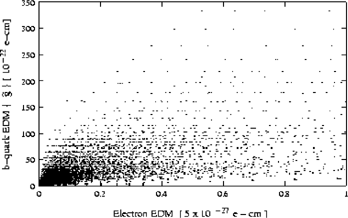
In the light of estimates made above, it is clear that the chargino (8) and gluino (4) contributions compete to dominate the $b$–quark EDM. To check the accuracy of these approximate results, we perform a scanning of the SUSY parameter space by varying all the mass parameters from $m_{t}$ up to ${\rm TeV}$ and $\tan\beta$ from 3 to 60 in accord with the collider bounds [16], recent LEP results [14], electron and neutron EDM upper bounds [6], and the experimentally allowed range of the $\mbox{BR}\left(B\rightarrow X_{s}\gamma\right)$ [13].

Depicted in Fig. 1 is the variation of the gluino contribution, $\left|{\cal{D}}_{b}^{\tilde{g}}\right|$ (in units of $10^{-22}~{}{\rm e-cm}$), to the bottom EDM as a function of the electron EDM (in units of the present experimental upper bound $5\times 10^{-27}~{}{\rm e-cm}$). It is clear from the figure that, ($i$) for most of the parameter space small values of the electron EDM are prefereed, for which $\left|{\cal{D}}_{b}^{\tilde{g}}\right|\sim 10^{-21}~{}{\rm e-cm}$, and and ($ii$) for certain portions of the parameter space, where the electron EDM tends to saturate its upper bound, $|{\cal{D}}_{b}^{\tilde{g}}$ takes on larger values so as to dominate the entire SUSY prediction; $\left|{\cal{D}}_{b}^{\tilde{g}}\right|_{max}\stackrel{{\scriptstyle<}}{{\scriptscriptstyle\sim}}3.5\times 10^{-20}~{}{\rm e-cm}$. Obviously these exact results agree with the approximate estimates made in (4).

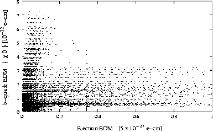
Similarly, in Fig. 2 is shown the scatter plot of the neutralino contribution, $\left|{\cal{D}}_{b}^{\chi^{0}}\right|$ (in units of $10^{-22}~{}{\rm e-cm}$), as a function of the the electron EDM. It is clear that, when the electron EDM is much smaller than the present bound, $\left|{\cal{D}}_{b}^{\chi^{0}}\right|$ remains mostly below $10^{-22}~{}{\rm e-cm}$, except for a small portion of the parameter space where it hits in the upper bound of $10^{-21}~{}{\rm e-cm}$. However, as the electron EDM takes on larger values $\left|{\cal{D}}_{b}^{\chi^{0}}\right|$ remains bounded around $10^{-22}~{}{\rm e-cm}$.

Figure 3: The same as Fig. 1, but for the chargino contribution, $\left|{\cal{D}}_{b}^{\chi^{\pm}}\right|$, to the bottom quark EDM (in units of $10^{-22}~{}{\rm e-cm}$).

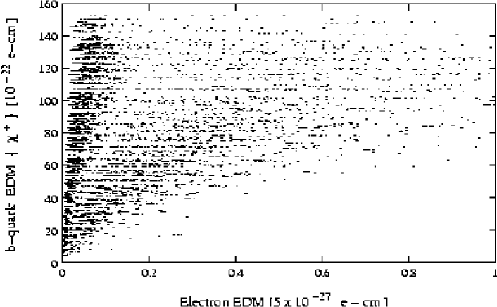
Fig. 3 shows is the scatter plot of the chargino contribution to the $b$–quark EDM, $\left|{\cal{D}}_{b}^{\chi^{\pm}}\right|$) (in units of $10^{-22}~{}{\rm e-cm}$) as the electron EDM varies in the experimentally allowed range. It is clear that, for the entire range of the electron EDM, the chargino contribution remains mostly around $10^{-20}~{}{\rm e-cm}$. That the chargino contribution, compared to the gluino one in Fig. 1, has a shaper edge around $1.6\times 10^{-20}~{}{\rm e-cm}$ is a direct consequence of the $\mbox{BR}\left(B\rightarrow X_{s}\gamma\right)$ constraint. Therefore, Figs. 1–3 imply that ($i$) the chargino contribution is dominant in most of the parameter space with a value in agreement with (8), ($ii$) the gluino contribution may exceed the chargino one in certain corners of the parameter space, ($iii$) the neutralino contribution remains of similar size as the two–loop contribution.

As a result, the naive estimates in (4), (8) and (10) for different SUSY contributions to the $b$–quark EDM are confirmed by a scanning of the SUSY parameter space as depicted in Figs. 1–3. Consequently, in minimal SUSY the $b$–quark EDM obeys the upper bound

$$\left|\left(\frac{{\cal{D}}_{b}}{e}\right)\right|\stackrel{{\scriptstyle<}}{{\scriptscriptstyle\sim}}10^{-20}\ {\rm cm}$$ (11)

which is due to the charginos for most of the SUSY parameter space.

In principle, as long as the theory at or above the mass scale of the fermion carries necessary sources for CP violation then the fermion possesses an EDM. Experimentally, there is no problem in measuring the EDM of the leptons as they can travel freely for sufficiently long distances. For light quarks $u$, $d$ and $s$, on the other hand, EDMs make sense due to the fact they are the constitutents of the nucleons.

It is still meaningful to calculate the EDM of the top quark as it can travel freely long enough distances before hadronization [22]. However, for the bottom quark the hadronization effects show up much faster and its EDM is not observable directly. For this reason, as in the EDMs of the $u$, $d$ and $s$ quarks, it is via the $b$–flavoured hadrons that the bottom EDM can cause experimentally observable effects. Therefore, the next section is devoted to the discussion of an experimentally testable process which is dominated by the bottom EDM calculated above.

3 $b$–quark EDM and ${}^{1}\mbox{P}_{1}$ Bottomonium

A short glance at the effective Lagrangian (1) which defines the EDM of the $b$–quark reveals that it is, in fact, identical to the coupling of photon to the ${}^{1}\mbox{P}_{1}\ (\equiv h_{b}(1\mbox{P})$ bottomonium. The quantum numbers, $J^{PC}=1^{+-}$, of this CP=-1 resonance coincide with those of the current density [23]

$$J_{\alpha}\left(\bar{b}b|{}^{1}\mbox{P}_{1}\right)=\overline{b}(x)\ {\stackrel{{\scriptstyle\longleftrightarrow}}{{\partial_{\alpha}}}}\ \gamma_{5}\ b(x)$$ (12)

whose coupling to photon gives the operator structure in (1). Presently, the experimental evidence for such CP–odd states is only limited to the observation [24] of the charmonium ${}^{1}{\mbox{P}}_{1}$ state as a resonance in the proton-antiproton annihilation, while the reported signal for the bottomonium state [25] has disappeared with increased statistics. In what follows, we discuss the formation of the ${}^{1}\mbox{P}_{1}$ bottomonium in $e^{+}e^{-}$ annihilation by an explicit calculation of the various contributions.

In the framework of the SM, $e^{+}e^{-}$ annihilation can yield a ${}^{1}\mbox{P}_{1}$ state through the $\gamma Z$ and $ZZ$ box diagrams. The former is the dominant process, and the relevant diagram is shown in Fig. 4 $(a)$. The CP parities of the initial, intermediate ($\gamma\,Z$), and final states must be identical, that is, the $e^{+}e^{-}$ sytem has $J^{PC}=1^{+-}$. Therefore, it is only the longitudinal part of the $Z$ boson which contributes to the process. In other words, the $Z$ boson exchange is equivalent to the exchange of the associated Goldstone boson, and a straightforward calculation gives the following effective Hamiltonian

$${\cal{H}}_{SM}\left({\small\mbox{CP}}\surd\right)=\frac{\alpha}{3\pi\sqrt{2}}\;G_{F}m_{e}m_{b}\;{\cal{B}}\ J_{\alpha}\left(\bar{b}b|{}^{1}\mbox{P}_{1}\right)\cdot J^{\alpha}\left(e^{+}e^{-}|{}^{1}\mbox{P}_{1}\right)$$ (13)

where the current $J_{\alpha}$ is defined in (12), and the box function ${\cal{B}}$ can be expressed in terms of the standard loop integarls [26]. For the characteristic scale of the problem, it behaves as

$${\cal{B}}\sim\frac{1}{M_{Z}^{2}\ m_{b}^{2}}\ \ln\left(\frac{m_{b}}{m_{e}}\right)~{}.$$ (14)

In minimal SUSY, with two Higgs doublets, there are two CP–odd spinless bosons, one of which becomes the longitudinal part of the $Z$ boson that induces the effective Hamiltonian (13). The other one is the physical CP–odd Higgs scalar, $A^{0}$. Due to its CP–odd nature this boson contributes to the formation of ${}^{1}\mbox{P}_{1}$ resonance in $e^{+}e^{-}$ annihilation. Replacing the $Z$ boson by $A^{0}$ in Fig. 4 $(a)$, the SUSY contributions to the CP–conserving effective Hamiltonian (13) turns out to be

$${\cal{H}}_{SUSY}\left({\small\mbox{CP}}\surd\right)=\tan^{2}\beta\ \times\ {\cal{H}}_{SM}\left({\small\mbox{CP}}\surd\right)\left[M_{Z}\leftrightarrow M_{A^{0}}\right]$$ (15)

which rises quadratically with $\tan\beta$. If there were no constraints coming from the electron EDM, this SUSY contribution would exceed the SM contribution (13) by three orders of magnitude for $\tan\beta\sim 60$ and $M_{A^{0}}\sim M_{Z}$. However, it is known that [12], for such a light $A^{0}$, $\tan\beta\stackrel{{\scriptstyle<}}{{\scriptscriptstyle\sim}}20$ so that a conservative figure for the SUSY enhancement hardly exceeds two orders of magnitude.

Figure 4: Formation of the ${}^{1}\mbox{P}_{1}$ bottomonium resonance in $e^{+}e^{-}$ scattering. The blob corresponds to the bottom quark EDM defined in (1).

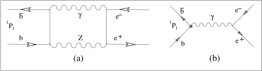
Besides the CP–conserving decay modes discussed above, the bottom quark EDM itself can trigger the formation of ${}^{1}\mbox{P}_{1}$ state in $e^{+}e^{-}$ annihilation. The relevant diagram is shown in Fig. 4 $(b$) where the grey blob stands for the insertion of the effective Lagrangian (1). Due to the CP violating nature of the EDMs it is clear that this transition violates CP so that $e^{+}e^{-}$ system does not need to be in the ${}^{1}\mbox{P}_{1}$ state. In fact the effective Hamiltonian following from this diagram reads as

$${\cal{H}}_{SUSY}\left({\small\mbox{CP}}\otimes\right)=\left(\frac{4\pi\alpha}{M_{h_{b}}^{2}}\right)\ \left(\frac{{\cal{D}}_{b}}{e}\right)\ J_{\alpha}\left(\bar{b}b|{}^{1}\mbox{P}_{1}\right)\cdot\left[e^{+}(x)\ \gamma^{\alpha}\ e^{-}(x)\right]$$ (16)

which clearly demonstrates the violation of the CP parity as the $e^{+}e^{-}$ system is in ${}^{3}\mbox{S}_{1}$ state having CP=+1.

A comparison of the CP–conserving (13,15) and CP–violating (16) transition amplitudes reveals that if the bottom quark EDM falls below the critical value

$$\left|\left(\frac{{\cal{D}}_{b}}{e}\right)\right|^{crit}\sim\frac{G_{F}m_{e}}{12\sqrt{2}\pi^{2}}\ \frac{M_{h_{b}}^{2}}{M_{Z}^{2}}\ \ln\frac{m_{b}}{m_{e}}\ \frac{\tan^{2}\beta\ M_{Z}^{2}}{M_{A^{0}}^{2}}\sim\frac{\tan^{2}\beta\ M_{Z}^{2}}{M_{A^{0}}^{2}}\times 10^{-25}~{}{\rm cm}$$ (17)

then experimentally formation of ${}^{1}\mbox{P}_{1}$ bottomonium resonance in $e^{+}e^{-}$ annihilation will not be informative at all. One notices that this critical bound, dominated by the SUSY CP–conserving transition (15), can be at most $10^{-23}~{}{\rm cm}$ which is below (11) by three orders of magnitude. This implies that the EDM of the bottom quark is the dominant piece in forming the ${}^{1}\mbox{P}_{1}$ bottomonium in $e^{+}e^{-}$ collisions, and observation of this resonance will become a direct probe of the soft phases in SUSY.

The non-observation of the ${}^{1}\mbox{P}_{1}$ state as a resonance in $e^{+}e^{-}$ annihilation puts a model–independent bound on the bottom EDM. Letting $R_{S}(r)$ and $R_{P}(r)$ [23] be the radial parts of the ${}^{3}\mbox{S}_{1}$ and ${}^{1}\mbox{P}_{1}$ levels respectively, and using (16), one finds

$$\left|\frac{{\cal{D}}_{b}}{e}\right|\approx\frac{|Q_{b}|}{\sqrt{12}}\left|\frac{R_{S}(0)}{R_{P}^{\prime}(0)}\right|\left|\frac{\sigma\left(e^{+}e^{-}\rightarrow{}^{1}\mbox{P}_{1}\right)}{\sigma\left(e^{+}e^{-}\rightarrow{}^{3}\mbox{S}_{1}\right)}\right|^{1/2}\stackrel{{\scriptstyle<}}{{\scriptscriptstyle\sim}}10^{-15}~{}{\rm cm}~{}.$$ (18)

The numerical value here conservatively assumes that present data exclude the ${}^{1}\mbox{P}_{1}$ resonance in $e^{+}e^{-}$ annihilation at the level of the formation cross section about $0.1$ of that for the $\Upsilon$ resonance. Clearly, this result is five orders of magnitude larger than the SUSY prediction (11), and if the actual experimental value turns out to be significantly larger than $10^{-20}$ cm, then certainly SUSY phases will not suffice to saturate it. Especially $\mbox{BR}\left(B\rightarrow X_{s}\gamma\right)$ will prohibit the enhancement of the bottom EDM beyond the bounds found in the previous section.

Another way of testing the bottom EDM is in decays of the ${}^{1}\mbox{P}_{1}$, provided that a sufficiently large sample of data for this resonance will ever be accumulated. The most direct way of searching and testing sources of CP violation beyond the SM will be through the decays of ${}^{1}\mbox{P}_{1}$ to hadronic final states with CP=+1. Like the well–known $K_{L}\rightarrow\pi\pi$ decay which has established nonvanishing CP violation in the Kaon system, decays of the form ${}^{1}\mbox{P}_{1}\rightarrow M\overline{M}$ ($M$ being a light hadron) will be a useful channel (See, for instance, [27] for analogous studies in charmonium system). Of course, for the ease of experimental detection, care should be payed to choosing appropriate final states where the CP–conserving SUSY transitions (15) are naturally suppressed.

For instance, the decays into charmed neutral mesons, ${}^{1}\mbox{P}_{1}\rightarrow\overline{D}D$, will proceed mainly with the bottom EDM since the CP–conserving SUSY contribution (15) goes like $\left(\tan\beta\right)^{0}$ as the $D$ meson side contains only up–type quarks. Moreover, for such a hadronic transition, the cromoelectric dipole moment (CEDM) of the $b$–quark provides the dominant mechanism for generating an $h_{b}D\bar{D}$ coupling[28]. Although this decay mode is preferred for enhancing the CP–violating transitions, there are various form factors involved in the hadronic amplitude which can suppress the signal significantly.

4 Conclusion

In this work we have computed the EDM of bottom quark in the minimal SUSY model with nonvanishing soft phases. The parameter space adopted is such that the EDMs of the neutron and electron are naturally suppressed in that they can arise only at two and higher loop levels via the quantum effects of scalar fermions and Higgs scalars [12]. The dominant contribution comes from the exchange of the CP–odd Higgs scalar.

However, one notices that in the same parameter space the third generation fermions, in particular the bottom quark, can have large EDMs generated by the one–loop quantum effects of the scalar fermions, gluinos, charginos and neutralinos. Indeed, in Sec. 2 we have shown, by both analytical and numerical methods, that for most of the parameter space the chargino contribution, which is directly correlated with the measured branching fraction [13] of the rare $B\rightarrow X_{s}\gamma$ decay, sets the upper bound on the $b$–quark EDM to be $\sim 10^{-20}~{}{\rm e-cm}$. For certain corners of the parameter space the gluino contribution can exceed this bound slightly with no order of magnitude enhancement, however.

After estimating the $b$–quark EDM in the minimal SUSY model we have discussed experimentally viable circumtances where it can have observable effects. In this context, the Sec. 3 has been devoted to a detailed discussion of the ${}^{1}\mbox{P}_{1}$ $\bar{b}b$ resonance formation in $e^{+}e^{-}$ annihilation. The explicit calculations show that the EDM of $b$–quark is the dominant effect in forming this CP–odd resonance, that is, the CP–conserving transition amplitudes are below the CP–violating one by three orders of magnitude. Hence, the very existence of a large bottom quark EDM, which is allowed in SUSY with explicit CP violation, is the driving force behind the possible observation of ${}^{1}\mbox{P}_{1}$ bottomonium resonance in $e^{+}e^{-}$ annihilations. Presently the experimental bound is five orders of magnitude above the SUSY prediction, and with increasing precision if experiment detects such a CP–odd resonance it will be a direct signal of the nonvanishing bottom EDM, or equivalently, the existence of the sources for CP violation beyond the SM such as SUSY.

However, the ultimate and most direct experimental observation of the $b$–quark EDM will be through decays of ${}^{1}\mbox{P}_{1}$ resonance to CP=+1 final states. In this context, one recalls the neutral charm mesons for which the CP–conserving transition is significantly smaller than that in the $e^{+}e^{-}$ annihilation by a factor of $1/\tan^{2}\beta$. Therefore, especially $\overline{D}D$ type final states will prove useful in probing the strength of the $b$–quark EDM.

If the improved experimental searches for the $h_{b}$ resonance in $e^{+}e^{-}$ annihilation yield a negative result, i.e. assuming that the present experimental precision (18) is improved down to the level of the critical value in (17) with no sign of ${}^{1}\mbox{P}_{1}$ resonance in $e^{+}e^{-}$ collisions, it is clear that experiment will be no more conclusive. Even if such a resonance is observed it will be necessary to search for its decay into CP=+1 states in order to establish the existence of a nonvanishing $b$–quark EDM. In case all such experimental efforts give negative results then there would remain only two options for SUSY with nonvanishing CP phases: $(i)$ The sparticles of all three generations are fairly above TeV so that SUSY cannot show up at the weak scale, or $(ii)$ Contributions of various sparticle loops must cancel so as to have EDMs of neutron, electron, muon, $b$–quark and atoms [29] all agree with the experimental bounds. The former makes weak scale SUSY unlikely [5] whereas the latter can require a finely tuned SUSY mass spectrum [4].

Appendix. Relevant Formulae

Loop Functions:

The loop functions entering the evaluation of $b\rightarrow X_{s}\gamma$ amplitude and $b$–quark EDM are given by

$$F_{0}(a) = \frac{a}{2(1-a)^{2}}\left[1+a+\frac{2a}{1-a}\ln a\right]$$

$$F_{\pm}(a) = \frac{a}{2(1-a)^{2}}\left[7-5a+\frac{2(3-2a)}{1-a}\ln a\right]$$

$$K_{1}^{8}(a) = \frac{1}{12(1-a)^{5}}\left[1-5a-2a^{2}-\frac{6a^{2}}{1-a}\ln a\right]$$

$$K_{1}^{7}(a) = Q_{t}K_{1}^{8}(a)+\frac{1}{12(1-a)^{5}}\left[2+5a-a^{2}-\frac{6a}{1-a}\ln a\right]$$ (A.1)

Mass Matrices:

Here we set the conventions for the mass matrices of squarks charginos, and neutralinos. The mass squared matrix of the top and bottom squarks ($f=t,b$) is given by

$$\widetilde{M}^{2}_{f}\ =\ \left(\begin{array}[]{cc}M^{2}_{\tilde{f}_{L}}\,+\,m^{2}_{f}\,+\,\cos 2\beta M^{2}_{Z}\,(I_{f}\,-\,Q_{f}s_{w}^{2})&m_{f}(A^{*}_{f}+\mu R_{f})\\ m_{f}(A_{f}+\mu^{*}R_{f})&M^{2}_{\tilde{f}_{R}}\,+\,m^{2}_{f}\,+\,\cos 2\beta M^{2}_{Z}\,Q_{f}s_{w}^{2}\end{array}\right)$$ (A.2)

where $R_{b}=R_{t}^{-1}=\tan\beta$. Being hermitian, $\widetilde{M}^{2}_{f}$ can be diagonalized via the unitary rotation

$$S_{f}^{\dagger}\,\widetilde{M}^{2}_{f}\,S_{f}=\mbox{diag.}\left(M^{2}_{\tilde{f}_{1}},M^{2}_{\tilde{f}_{2}}\right)~{},$$ (A.3)

with $M_{\tilde{f}_{1}}<M_{\tilde{f}_{2}}$.

The mass matrix of charginos

$$M^{-}\ =\ \left(\begin{array}[]{cc}M_{2}&-\sqrt{2}M_{W}\cos\beta\\ -\sqrt{2}M_{W}\sin\beta&\mu\end{array}\right)$$ (A.6)

can be diagnalized by a biunitary rotation

$$C_{R}^{\dagger}M^{-}C_{L}=\mbox{diag.}\left(M_{\chi^{\pm}_{1}},M_{\chi^{\pm}_{2}}\right)~{},$$ (A.7)

where $C_{R}$ and $C_{L}$ are unitary matrices, and $M_{\chi^{\pm}_{1}}<M_{\chi^{\pm}_{2}}$.

Finally, the neutralinos are described by a $4\times 4$ mass matrix

$$M^{0}\ =\ \left(\begin{array}[]{cccc}M_{1}&0&M_{Z}s_{w}\cos\beta&-M_{Z}s_{w}\sin\beta\\ 0&M_{2}&-M_{Z}c_{w}\cos\beta&M_{Z}c_{w}\sin\beta\\ M_{Z}s_{w}\cos\beta&-M_{Z}c_{w}\cos\beta&0&-\mu\\ -M_{Z}s_{w}\sin\beta&M_{Z}c_{w}\sin\beta&-\mu&0\end{array}\right)$$ (A.12)

which can be diagonalized via

$$C_{0}^{T}M^{0}C_{0}=\mbox{diag.}\left(M_{\chi^{0}_{1}},\cdots,M_{\chi^{0}_{4}}\right)$$ (A.13)

where $M_{\chi^{0}_{1}}<\cdots<M_{\chi^{0}_{4}}$.

Vertex Coefficients:

Here we list down the vertex coefficients entering the evaluation of the Wilson coefficient $C_{7}$ and the $b$–quark EDM:

$$\Gamma_{\tilde{g}}^{k} = S_{{b}{1k}}^{*}S_{{b}{2k}}~{},$$

$$\Gamma_{\chi^{0}}^{ki} = \frac{c_{w}^{2}}{s_{w}^{2}}\ \left[C_{{0}{2i}}S_{{b}{1k}}^{*}-\frac{s_{w}}{3c_{w}}C_{{0}{1i}}S_{{b}{1k}}^{*}-\frac{h_{b}}{g_{2}}C_{{0}{3i}}S_{{b}{2k}}^{*}\right]\left[\frac{s_{w}}{3c_{w}}C_{{0}{1i}}S_{{b}{2k}}+\frac{h_{b}}{g_{2}}C_{{0}{3i}}S_{{b}{1k}}\right]~{},$$

$$\Gamma_{\chi^{\pm}}^{kj} = \frac{h_{b}}{g_{2}}\left[C_{{R}{1j}}^{*}S_{{t}{1k}}^{*}-\frac{h_{t}}{g_{2}}C_{{R}{2j}}^{*}S_{{t}{2k}}^{*}\right]C_{{L}{2j}}S_{{t}{1k}}~{},$$ (A.14)

where the ranges of the indices are $k=1,2,\;i=1,\cdots,4$, and $j=1,2$. In all the formulae above, $s_{w}\equiv\sin\theta_{w}$, $c_{w}\equiv\cos\theta_{w}$ with $\theta_{w}$ being the Weinberg angle.

References

- [1] M. Dugan, B. Grinstein and L. Hall, Nucl. Phys. B255, 413 (1985); M. J. Duncan, Nucl. Phys. B221, 285 (1983); J. F. Donoghue, H. P. Nilles and D. Wyler, Phys. Lett. B128, 55 (1983); A. Bouquet, J. Kaplan and C. A. Savoy, Phys. Lett. B148, 69 (1984).
- [2] D. A. Demir, Phys. Rev. D60, 055006 (1999) [hep-ph/9901389]; Phys. Rev. D60, 095007 (1999) [hep-ph/9905571]; Phys. Lett. B465, 177 (1999) [hep-ph/9809360]; A. Pilaftsis and C. E. Wagner, Nucl. Phys. B553, 3 (1999) [hep-ph/9902371]; M. Carena, J. Ellis, A. Pilaftsis and C. E. Wagner, Nucl. Phys. B586, 92 (2000) [hep-ph/0003180]; A. Pilaftsis, Phys. Lett. B435, 88 (1998) [hep-ph/9805373]; S. Y. Choi, M. Drees and J. S. Lee, Phys. Lett. B481, 57 (2000) [hep-ph/0002287]; T. Ibrahim and P. Nath, hep-ph/0008237.
- [3] J. Ellis, S. Ferrara and D. V. Nanopoulos, Phys. Lett. B114, 231 (1982); J. Polchinski and M. B. Wise, Phys. Lett. B125, 393 (1983); F. del Aguila, M. B. Gavela, J. A. Grifols and A. Mendez, Phys. Lett. B126, 71 (1983); D. V. Nanopoulos and M. Srednicki, Phys. Lett. B128, 61 (1983); T. Falk, K. A. Olive and M. Srednicki, Phys. Lett. B354, 99 (1995) [hep-ph/9502401]. S. Pokorski, J. Rosiek and C. A. Savoy, Nucl. Phys. B570, 81 (2000) [hep-ph/9906206]; E. Accomando, R. Arnowitt and B. Dutta, Phys. Rev. D61, 115003 (2000) [hep-ph/9907446]; J. Dai, H. Dykstra, R. G. Leigh, S. Paban and D. Dicus, Phys. Lett. B237, 216 (1990); S. Weinberg, Phys. Rev. Lett. 63, 2333 (1989).
- [4] T. Ibrahim and P. Nath, Phys. Lett. B418, 98 (1998) [hep-ph/9707409]; Phys. Rev. D57, 478 (1998) [hep-ph/9708456]; M. Brhlik, G. J. Good and G. L. Kane, Phys. Rev. D59, 115004 (1999) [hep-ph/9810457]; T. Falk and K. A. Olive, Phys. Lett. B439, 71 (1998) [hep-ph/9806236]; Phys. Lett. B375, 196 (1996) [hep-ph/9602299].
- [5] P. Nath, Phys. Rev. Lett. 66 (1991) 2565; Y. Kizukuri and N. Oshimo, Phys. Rev. D45, 1806 (1992); Phys. Rev. D46, 3025 (1992).
- [6] P. G. Harris et al., Phys. Rev. Lett. 82, 904 (1999).
- [7] D. A. Demir and E. Ma, Phys. Rev. D62, 111901 (2000) [hep-ph/0004148]; D. A. Demir, E. Ma and U. Sarkar, J. Phys. G26, L117 (2000) [hep-ph/0005288].
- [8] R. D. Peccei and H. R. Quinn, Phys. Rev. Lett. 38, 1440 (1977); M. A. Shifman, A. I. Vainshtein and V. I. Zakharov, Nucl. Phys. B166, 493 (1980); J. E. Kim, Phys. Rev. Lett. 43, 103 (1979).
- [9] D. A. Demir, Phys. Rev. D62, 075003 (2000) [hep-ph/9911435]; S. Dimopoulos and S. Thomas, Nucl. Phys. B465, 23 (1996) [hep-ph/9510220].
- [10] G.F. Giudice and S. Dimopoulos, Phys. Lett. B357, 573 (1995); G. Dvali and A. Pomarol, Phys. Rev. Lett. 77, 3728 (1996); A.G. Cohen, D.B. Kaplan, and A.E. Nelson, Phys. Lett. B388, 588 (1996); P. Binetruy and E. Dudas, Phys. Lett. B389, 503 (1996).
- [11] S. M. Barr and A. Zee, Phys. Rev. Lett. 65, 21 (1990);
- [12] D. Chang, W. Keung and A. Pilaftsis, Phys. Rev. Lett. 82, 900 (1999) [hep-ph/9811202]; A. Pilaftsis, Phys. Lett. B471, 174 (1999) [hep-ph/9909485]; D. Chang, W. Chang and W. Keung, Phys. Lett. B478, 239 (2000) [hep-ph/9910465].
- [13] S. Ahmed et al. [CLEO Collaboration], hep-ex/9908022; T. E. Coan et al. [CLEO Collaboration], hep-ex/0010075.
- [14] J. Ellis, talk at Thirty Years of Supersymmetry, October 13 – 15, 2000; Ch. Tully, Higgs Working Group Report for LEPC, September 2000.
- [15] E. P. Shabalin, Phys. Lett. B109, 490 (1982); Sov. J. Nucl. Phys. 32, 228 (1980); N. G. Deshpande, G. Eilam and W. L. Spence, Phys. Lett. B108, 42 (1982); J. O. Eeg and I. Picek, Nucl. Phys. B244, 77 (1984).
- [16] M. Schmitt, (Particle Data Group), Euro. Phys. J. C15, 826 (2000).
- [17] M. Aoki, G. Cho and N. Oshimo, Nucl. Phys. B554, 50 (1999) [hep-ph/9903385].
- [18] M. Misiak, hep-ph/0009033; K. Chetyrkin, M. Misiak and M. Munz, Phys. Lett. B400, 206 (1997) [hep-ph/9612313].
- [19] D. A. Demir, A. Masiero and O. Vives, Phys. Rev. Lett. 82, 2447 (1999) [hep-ph/9812337]; S. Baek and P. Ko, Phys. Rev. Lett. 83, 488 (1999) [hep-ph/9812229].
- [20] A. L. Kagan and M. Neubert, Phys. Rev. D58, 094012 (1998) [hep-ph/9803368].
- [21] D. A. Demir, A. Masiero and O. Vives, Phys. Rev. D61, 075009 (2000) [hep-ph/9909325]; Phys. Lett. B479, 230 (2000) [hep-ph/9911337].
- [22] P. Poulose and S. D. Rindani, Phys. Rev. D57, 5444 (1998) [hep-ph/9709225]; S. Y. Choi and K. Hagiwara, Phys. Lett. B359, 369 (1995) [hep-ph/9506430].
- [23] V. A. Novikov, L. B. Okun, M. A. Shifman, A. I. Vainshtein, M. B. Voloshin and V. I. Zakharov, Phys. Rept. 41, 1 (1978).
- [24] T. A. Armstrong et al. [E760 Collaboration], Phys. Rev. Lett. 69, 2337 (1992).
- [25] T. Bowcock et al. [CLEO Collaboration], Phys. Rev. Lett. 58, 307 (1987).
- [26] G. ’t Hooft and M. Veltman, Nucl. Phys. B153, 365 (1979); G. Passarino and M. Veltman, Nucl. Phys. B160, 151 (1979).
- [27] F. Murgia, Phys. Rev. D54, 3365 (1996) [hep-ph/9601386]; A. D. Martin, M. G. Olsson and W. J. Stirling, Phys. Lett. B147, 203 (1984).
- [28] Y. Fujiwara, Prog. Theor. Phys. 89, 455 (1993).
- [29] T. Falk, K. A. Olive, M. Pospelov and R. Roiban, Nucl. Phys. B560, 3 (1999) [hep-ph/9904393].