Leading Isgur-Wise form factor of $\Lambda_{b}\to\Lambda_{c1}$ transition using QCD sum rules

Abstract

The leading Isgur-Wise form factor $\xi(y)$ parametrizing the semileptonic transitions $\Lambda_{b}\to\Lambda^{1/2}_{c1}\ell\bar{\nu}$ and $\Lambda_{b}\to\Lambda^{3/2}_{c1}\ell\bar{\nu}$ is calculated by using the QCD sum rules in the framework of heavy quark effective theory, where $\Lambda^{1/2}_{c1}$ and $\Lambda^{3/2}_{c1}$ is the orbitally excited charmed baryon doublet with $J^{P}=(1^{-}/2,3^{-}/2)$. The interpolating currents with transverse covariant derivative are adopted for $\Lambda^{1/2}_{c1}$ and $\Lambda^{3/2}_{c1}$ in the analysis. The slope parameter $\rho^{2}$ in linear approximation of the Isgur-Wise function is obtained to be $\rho^{2}=2.01$, and the interception to be $\xi(1)=0.29$. The decay branching ratios are estimated.

I Introduction

The ground state bottom baryon $\Lambda_{b}$ weak decays [1] provide a testing ground for the standard model (SM). They reveal some important features of the physics of bottom quark. The experimental data on them are accumulating, and waiting for reliable theoretical calculations. The main difficulties in the SM calculations, however, are due to the poor understanding of the nonperturbative aspects of the strong interaction (QCD). The heavy quark effective theory (HQET) based on the heavy quark symmetry provides a model-independent method for analyzing heavy hadrons containing a single heavy quark [2]. It allows us to expand the physical quantity in powers of $1/m_{Q}$ systematically, where $m_{Q}$ is the heavy quark mass. Within this framework, the classification of the $\Lambda_{b}$ exclusive weak decay form factors has been simplified greatly. The decays $\Lambda_{b}\to\Lambda_{c}l{\bar{\nu}}$ [3], $\Lambda_{b}\to\Sigma_{c}^{(*)}l{\bar{\nu}}$ [4], $\Lambda_{b}\to\Sigma_{c}^{(*)}\pi l{\bar{\nu}}$ [5], $\Lambda_{b}\to p(\Lambda)$ [6] have been studied.

With the discovery of the orbitally excited charmed baryons $\Lambda_{c}(2593)$ and $\Lambda_{c}(2625)$ [7], it would be interesting to investigate the $\Lambda_{b}$ semileptonic decays into these baryons. From the phenomenological point of view, these semileptonic transitions are interesting, since in principle they may account for a sizeable fraction of the inclusive semileptonic rate of $\Lambda_{b}$ decay.

The properties of excited baryons have attracted attention in recent years. Investigation on them will extend our ability in the application of QCD. It can also help us foresee other excited heavy baryons undiscovered yet. The heavy quark symmetry [2] is a useful tool to classify the hadronic spectroscopy containing a heavy quark $Q$. In the infinite mass limit, the spin and parity of the heavy quark and that of the light degrees of freedom are separately conserved. Coupling the spin of light degrees of freedom $j_{\ell}$ with the spin of heavy quark $s_{Q}=1/2$ yields a doublet with total spin $J=j_{\ell}\pm 1/2$ (or a singlet if $j_{\ell}=0$). This classification can be applied to the $\Lambda_{Q}$-type baryons. For the charmed baryons the ground state $\Lambda_{c}$ contains light degrees of freedom with spin-parity $j_{\ell}^{P}=0^{+}$, being a singlet. The excited states with $j_{\ell}^{P}=1^{-}$ are spin symmetry doublet with $J^{P}$($1^{-}/2$,$3^{-}/2$). The lowest states of such excited charmed states, $\Lambda^{1/2}_{c1}$ and $\Lambda^{3/2}_{c1}$, have been observed and are identified with $\Lambda_{c}(2593)$ and $\Lambda_{c}(2625)$ respectively [7].

The semileptonic $\Lambda_{b}$ decay rate to the excited charmed baryon is determined by corresponding hadronic matrix elements of the weak axial-vector and vector currents. The matrix elements of the vector and axial currents ($V_{\mu}={\bar{c}}\gamma_{\mu}b$ and $A_{\mu}={\bar{c}}\gamma_{\mu}\gamma_{5}b$) between the $\Lambda_{b}$ and $\Lambda^{1/2}_{c1}$ or $\Lambda^{3/2}_{c1}$ can be parametrized in terms of fourteen form factors:

$$\frac{\langle\Lambda_{c1}^{1/2}(v^{\prime},s^{\prime})|V_{\mu}|\Lambda_{b}(v,s)\rangle}{\sqrt{4M_{\Lambda_{c1}(1/2)}M_{\Lambda_{b}}}} = {\bar{u}}_{\Lambda_{c1}}(v^{\prime},s^{\prime})\Big{[}F_{1}\gamma_{\mu}+F_{2}v_{\mu}+F_{3}v^{\prime}_{\mu}\Big{]}\gamma_{5}u_{\Lambda_{b}}(v,s)~{},$$ (2)

$$\frac{\langle\Lambda_{c1}^{1/2}(v^{\prime},s^{\prime})|A_{\mu}|\Lambda_{b}(v,s)\rangle}{\sqrt{4M_{\Lambda_{c1}(1/2)}M_{\Lambda_{b}}}} = {\bar{u}}_{\Lambda_{c1}}(v^{\prime},s^{\prime})\Big{[}G_{1}\gamma_{\mu}+G_{2}v_{\mu}+G_{3}v^{\prime}_{\mu}\Big{]}u_{\Lambda_{b}}(v,s)~{},$$ (3)

$$\frac{\langle\Lambda_{c1}^{3/2}(v^{\prime},s^{\prime})|V_{\mu}|\Lambda_{b}(v,s)\rangle}{\sqrt{4M_{\Lambda_{c1}(3/2)}M_{\Lambda_{b}}}} = {\bar{u}}^{\alpha}_{\Lambda_{c1}}(v^{\prime},s^{\prime})\Big{[}v_{\alpha}(K_{1}\gamma_{\mu}+K_{2}v_{\mu}+K_{3}v^{\prime}_{\mu})+K_{4}g_{\alpha\mu}\Big{]}u_{\Lambda_{b}}(v,s)~{},$$ (4)

$$\frac{\langle\Lambda_{c1}^{3/2}(v^{\prime},s^{\prime})|A_{\mu}|\Lambda_{b}(v,s)\rangle}{\sqrt{4M_{\Lambda_{c1}(3/2)}M_{\Lambda_{b}}}} = {\bar{u}}^{\alpha}_{\Lambda_{c1}}(v^{\prime},s^{\prime})\Big{[}v_{\alpha}(N_{1}\gamma_{\mu}+N_{2}v_{\mu}+N_{3}v^{\prime}_{\mu})+N_{4}g_{\alpha\mu}\Big{]}\gamma_{5}u_{\Lambda_{b}}(v,s)~{},$$ (5)

where $v(v^{\prime})$ and $s(s^{\prime})$ are the four-velocity and spin of $\Lambda_{b}(\Lambda_{c1})$, respectively. And the form factors $F_{i}$, $G_{i}$, $K_{i}$ and $N_{i}$ are functions of $y=v\cdot v^{\prime}$. In the limit $m_{Q}\to\infty$, all the form factors are related to one independent universal form factor $\xi(y)$ called Isgur-Wise (IW) function [8]. Extensive investigation in [9] further shows that the leading $1/m_{Q}$ correction of the form factors at zero recoil can be calculated in a model-independent way in terms of the masses of charmed baryon states. A convenient way to evaluate hadronic matrix elements is by introducing interpolating fields in HQET developed in Ref. [10] to parametrize the matrix elements in Eqs. (I). With the aid of this method the matrix element can be written as [9]

$${\bar{c}}\Gamma b={\bar{h}}^{(c)}_{v^{\prime}}\Gamma h^{(b)}_{v}=\xi(y)v_{\alpha}{\bar{\psi}}^{\alpha}_{v^{\prime}}\Gamma\psi_{v}~{}$$ (6)

at leading order in $1/m_{Q}$ and $\alpha_{s}$, where $\Gamma$ is any collection of $\gamma$-matrices. The ground state field, $\psi_{v}$, destroys the $\Lambda_{b}$ baryon with four-velocity $v$; the spinor field $\psi^{\alpha}_{v}$ is given by

$$\psi^{\alpha}_{v}=\psi^{3/2\alpha}_{v}+\frac{1}{\sqrt{3}}(\gamma^{\alpha}+v^{\alpha})\gamma_{5}\psi^{1/2}_{v}~{},$$ (7)

where $\psi^{1/2}_{v}$ is the ordinary Dirac spinor and $\psi^{3/2\alpha}_{v}$ is the spin 3/2 Rarita-Schwinger spinor, they destroy $\Lambda^{1/2}_{c1}$ and $\Lambda^{3/2}_{c1}$ baryons with four-velocity $v$, respectively. To be explicit,

$$F_{1} = \frac{1}{\sqrt{3}}(y-1)~{}\xi(y)~{},~{}~{}~{}G_{1}=\frac{1}{\sqrt{3}}(y+1)~{}\xi(y)~{},$$ (8)

$$F_{2} = G_{2}=-\frac{2}{\sqrt{3}}~{}\xi(y)~{},~{}~{}~{}~{}~{}K_{1}=N_{1}=\xi(y)~{},$$ (10)

$$~{}~{}~{}~{}~{}~{}~{}~{}~{}~{}~{}~{}~{}~{}~{}~{}~{}({\rm others})=0~{}.$$

In general, the IW form factor is a decreasing function of the four velocity transfer $y$. Since the kinematically allowed region of $y$ for heavy to heavy transition is very narrow around unity,

$$1\leq y\leq\frac{M_{\Lambda_{b}}^{2}+M_{\Lambda_{c1}}^{2}}{2M_{\Lambda_{b}}M_{\Lambda_{c1}}}\simeq 1.2~{},$$ (11)

it is convenient to approximate the IW function linearly

$$\xi(y)=\xi(1)(1-\rho^{2}(y-1))~{},$$ (12)

where $\rho^{2}$ is the slope parameter which characterizes the shape of the IW function.

To obtain detailed predictions for the hadrons, however, some nonperturbative QCD methods are required. We adopt QCD sum rules [11] in this work. QCD sum rule is a powerful nonperturbative method based on QCD [11]. It takes into account the nontrivial QCD vacuum, parametrized by various vacuum condensates, to describe the nonperturbative nature. In QCD sum rule, hadronic observables are calculable by evaluating two- or three-point correlation functions. The hadronic currents for constructing the correlation functions are expressed by the interpolating fields. The static properties of $\Lambda_{b}$ and $\Lambda_{c1}$ ($\Lambda_{c1}$ denotes the generic $j_{\ell}^{P}=1^{-}$ charmed state) have been studied with QCD sum rules in the HQET in [12] and [13, 14], respectively. The aim of this work is to calculate the leading IW function $\xi(y)$ using the QCD sum rules.

In the next Section, the QCD sum rule calculations for $\xi(y)$ are given. Numerical results and discussions are in Sec. III. Summary of this work is in Sec. IV.

II The QCD Sum Rule Calculations

As a starting point, consider the interpolating field of heavy baryons. The heavy baryon current is generally expressed as

$$j^{v}_{J,P}(x)=\epsilon_{ijk}[q^{iT}(x)C\Gamma_{J,P}\tau q^{j}(x)]\Gamma^{\prime}_{J,P}h^{k}_{v}(x)~{},$$ (13)

where $i,~{}j,~{}k$ are the color indices, $C$ is the charge conjugation matrix, and $\tau$ is the isospin matrix while $q(x)$ is a light quark field. $\Gamma_{J,P}$ and $\Gamma^{\prime}_{J,P}$ are some gamma matrices which describe the structure of the baryon with spin-parity $J^{P}$. Usually $\Gamma$ and $\Gamma^{\prime}$ with least number of derivatives are used in the QCD sum rule method. The sum rules then have better convergence in the high energy region and often have better stability. For the ground state heavy baryon, we use $\Gamma_{1/2,+}=\gamma_{5}$, $\Gamma^{\prime}_{1/2,+}=1$. In the previous work [13], two kinds of interpolating fields are introduced to represent the excited heavy baryon. In this work, we find that only the interpolating field of transverse derivative is adequate for the analysis. Nonderivative interpolating field results in a vanishing perturbative contribution. The choice of $\Gamma$ and $\Gamma^{\prime}$ with derivatives for the $\Lambda_{c1}^{1/2}$ and $\Lambda_{c1}^{3/2}$ is then

$$\Gamma_{1/2,-}=(a+b\mathchoice{\ooalign{$\hfil\displaystyle\mkern 0.0mu/\hfil$\crcr$\displaystyle v$}}{\ooalign{$\hfil\textstyle\mkern 0.0mu/\hfil$\crcr$\textstyle v$}}{\ooalign{$\hfil\scriptstyle\mkern 0.0mu/\hfil$\crcr$\scriptstyle v$}}{\ooalign{$\hfil\scriptscriptstyle\mkern 0.0mu/\hfil$\crcr$\scriptscriptstyle v$}})\gamma_{5}~{},~{}~{}~{}~{}~{} \Gamma^{\prime}_{1/2,-}=\frac{i{\overleftarrow{\mathchoice{\ooalign{$\hfil\displaystyle\mkern 0.0mu/\hfil$\crcr$\displaystyle D$}}{\ooalign{$\hfil\textstyle\mkern 0.0mu/\hfil$\crcr$\textstyle D$}}{\ooalign{$\hfil\scriptstyle\mkern 0.0mu/\hfil$\crcr$\scriptstyle D$}}{\ooalign{$\hfil\scriptscriptstyle\mkern 0.0mu/\hfil$\crcr$\scriptscriptstyle D$}}}_{t}}}{M}\gamma_{5}~{},$$ (30)

$$\Gamma_{3/2,-}=(a+bv/)\gamma_{5}~{},~{}~{}~{}~{}~{} \Gamma^{\prime}_{3/2,-}=\frac{1}{3M}(i{\overleftarrow{D}}^{\mu}_{t}+i{\overleftarrow{\mathchoice{\ooalign{$\hfil\displaystyle\mkern 0.0mu/\hfil$\crcr$\displaystyle D$}}{\ooalign{$\hfil\textstyle\mkern 0.0mu/\hfil$\crcr$\textstyle D$}}{\ooalign{$\hfil\scriptstyle\mkern 0.0mu/\hfil$\crcr$\scriptstyle D$}}{\ooalign{$\hfil\scriptscriptstyle\mkern 0.0mu/\hfil$\crcr$\scriptscriptstyle D$}}}_{t}}\;\gamma^{\mu}_{t})~{},$$ (39)

where a transverse vector $A^{\mu}_{t}$ is defined to be $A^{\mu}_{t}\equiv A^{\mu}-v^{\mu}v\cdot A$, and $M$ in Eq. (39) is some hadronic mass scale. $a$, $b$ are arbitrary numbers between 0 and 1.

The baryonic decay constants in the HQET are defined as follows,

$$\langle 0|j^{v}_{1/2,+}|\Lambda_{b}\rangle = f_{\Lambda_{b}}\psi_{v}~{},$$ (41)

$$\langle 0|j^{v}_{1/2,-}|\Lambda_{c1}^{1/2}\rangle = f_{1/2}\psi^{1/2}_{v}~{},$$ (42)

$$\langle 0|j^{v\mu}_{3/2,-}|\Lambda_{c1}^{3/2}\rangle = \frac{1}{\sqrt{3}}f_{3/2}\psi^{3/2\mu}_{v}\;,$$ (43)

where $f_{1/2}$ and $f_{3/2}$ are equivalent since $\Lambda_{c1}^{1/2}$ and $\Lambda_{c1}^{3/2}$ belong to the same doublet with $j_{\ell}^{P}=1^{-}$. The QCD sum rule calculations give [12]

$$f_{\Lambda_{b}}^{2}e^{-{\bar{\Lambda}}/T}=\frac{1}{20\pi^{4}}\int_{0}^{\omega_{c}}d\omega\omega^{5}e^{-\omega/T}+\frac{1}{6}\langle{\bar{q}}q\rangle^{2}e^{-m_{0}^{2}/8T^{2}}+\frac{\langle\alpha_{s}GG\rangle}{32\pi^{3}}T^{2}~{},$$ (44)

and [13]

$$f_{1/2}^{2}e^{-{\bar{\Lambda}}^{\prime}/T^{\prime}} = \int_{0}^{\omega_{c}^{\prime}}d\omega\frac{3N_{c}!}{4\pi^{4}\cdot 7!}\omega^{7}(24a^{2}+40b^{2})e^{-\omega/T^{\prime}}+\frac{\langle\alpha_{s}GG\rangle}{32\pi^{3}}T^{\prime 4}(-a^{2}+b^{2})$$ (46)

$$+\frac{N_{c}!}{2\pi^{2}}\Big{[}\langle{\bar{q}}q\rangle T^{\prime 5}(16ab)-\langle{\bar{q}}g\sigma\cdot Gq\rangle T^{\prime 3}ab\Big{]}-\frac{\langle{\bar{q}}g\sigma\cdot Gq\rangle}{4\pi^{2}}T^{\prime 3}(3ab)~{}.$$

In the above equations, $T^{(\prime)}$ are the Borel parameters and $\omega_{c}^{(\prime)}$ are the continuum thresholds, and $N_{c}=3$ is the color number. In the heavy quark limit, the mass parameters $\bar{\Lambda}$ and $\bar{\Lambda}^{\prime}$ are defined as

$${\bar{\Lambda}}^{\prime}=M_{\Lambda_{Q1}}-m_{Q}~{},~{}~{}~{}~{}~{}{\bar{\Lambda}}=M_{\Lambda_{Q}}-m_{Q}~{}.$$ (47)

In order to get the QCD sum rule for the IW function, one studies the analytic properties of the three-point correlators

$$\Xi^{\mu}(\omega,\omega^{\prime},y) = i^{2}\int d^{4}xd^{4}z~{}e^{i(k^{\prime}\cdot x-k\cdot z)}\langle 0|{\cal T}~{}j^{v^{\prime}}_{1/2,-}(x)~{}{\bar{h}}^{(c)}_{v^{\prime}}(0)\Gamma^{\mu}h^{(b)}_{v}(0)~{}{\bar{j}}^{v}_{1/2,+}(z)|0\rangle$$ (74)

$$\quad=\Xi(\omega,\omega^{\prime},y)\;(\mathchoice{\ooalign{$\hfil\displaystyle\mkern 0.0mu/\hfil$\crcr$\displaystyle v$}}{\ooalign{$\hfil\textstyle\mkern 0.0mu/\hfil$\crcr$\textstyle v$}}{\ooalign{$\hfil\scriptstyle\mkern 0.0mu/\hfil$\crcr$\scriptstyle v$}}{\ooalign{$\hfil\scriptscriptstyle\mkern 0.0mu/\hfil$\crcr$\scriptscriptstyle v$}}+y)\gamma_{5}\;\frac{1+\mathchoice{\ooalign{$\hfil\displaystyle\mkern 0.0mu/\hfil$\crcr$\displaystyle v$}}{\ooalign{$\hfil\textstyle\mkern 0.0mu/\hfil$\crcr$\textstyle v$}}{\ooalign{$\hfil\scriptstyle\mkern 0.0mu/\hfil$\crcr$\scriptstyle v$}}{\ooalign{$\hfil\scriptscriptstyle\mkern 0.0mu/\hfil$\crcr$\scriptscriptstyle v$}}^{\prime}}{2}\Gamma^{\mu}\frac{1+\mathchoice{\ooalign{$\hfil\displaystyle\mkern 0.0mu/\hfil$\crcr$\displaystyle v$}}{\ooalign{$\hfil\textstyle\mkern 0.0mu/\hfil$\crcr$\textstyle v$}}{\ooalign{$\hfil\scriptstyle\mkern 0.0mu/\hfil$\crcr$\scriptstyle v$}}{\ooalign{$\hfil\scriptscriptstyle\mkern 0.0mu/\hfil$\crcr$\scriptscriptstyle v$}}}{2}\;,$$

$$\Xi^{\alpha\mu}(\omega,\omega^{\prime},y) = i^{2}\int d^{4}xd^{4}z~{}e^{i(k^{\prime}\cdot x-k\cdot z)}\langle 0|{\cal T}~{}j^{v^{\prime}\alpha}_{3/2,-}(x)~{}{\bar{h}}^{(c)}_{v^{\prime}}(0)\Gamma^{\mu}h^{(b)}_{v}(0)~{}{\bar{j}}^{v}_{1/2,+}(z)|0\rangle$$ (100)

$$\quad=\Xi(\omega,\omega^{\prime},y)\;[(-v^{\alpha}+yv^{{}^{\prime}\alpha}+\frac{1}{3}(\gamma^{\alpha}+v^{{}^{\prime}\alpha})\;(\mathchoice{\ooalign{$\hfil\displaystyle\mkern 0.0mu/\hfil$\crcr$\displaystyle v$}}{\ooalign{$\hfil\textstyle\mkern 0.0mu/\hfil$\crcr$\textstyle v$}}{\ooalign{$\hfil\scriptstyle\mkern 0.0mu/\hfil$\crcr$\scriptstyle v$}}{\ooalign{$\hfil\scriptscriptstyle\mkern 0.0mu/\hfil$\crcr$\scriptscriptstyle v$}}-y)]\;\frac{1+\mathchoice{\ooalign{$\hfil\displaystyle\mkern 0.0mu/\hfil$\crcr$\displaystyle v$}}{\ooalign{$\hfil\textstyle\mkern 0.0mu/\hfil$\crcr$\textstyle v$}}{\ooalign{$\hfil\scriptstyle\mkern 0.0mu/\hfil$\crcr$\scriptstyle v$}}{\ooalign{$\hfil\scriptscriptstyle\mkern 0.0mu/\hfil$\crcr$\scriptscriptstyle v$}}^{\prime}}{2}\Gamma^{\mu}\frac{1+\mathchoice{\ooalign{$\hfil\displaystyle\mkern 0.0mu/\hfil$\crcr$\displaystyle v$}}{\ooalign{$\hfil\textstyle\mkern 0.0mu/\hfil$\crcr$\textstyle v$}}{\ooalign{$\hfil\scriptstyle\mkern 0.0mu/\hfil$\crcr$\scriptstyle v$}}{\ooalign{$\hfil\scriptscriptstyle\mkern 0.0mu/\hfil$\crcr$\scriptscriptstyle v$}}}{2}\;,$$

where $\Gamma^{\mu}=\gamma^{\mu}$ or $\gamma^{\mu}\gamma_{5}$. The variables $k$, $k^{\prime}$ denote residual “off-shell” momenta which are related to the momenta $P$ of the heavy quark in the initial state and $P^{\prime}$ in the final state by $k=P-m_{Q}v$, $k^{\prime}=P^{\prime}-m_{Q^{\prime}}v^{\prime}$, respectively.

The coefficient $\Xi(\omega,\omega^{\prime},y)$ in (II) is an analytic function in the “off-shell energies” $\omega=v\cdot k$ and $\omega^{\prime}=v^{\prime}\cdot k^{\prime}$ with discontinuities for positive values of these variables. It furthermore depends on the velocity transfer $y=v\cdot v^{\prime}$, which is fixed at its physical region for the process under consideration. By saturating with physical intermediate states in HQET, one finds the hadronic representation of the correlators as following

$$\Xi_{\rm hadron}(\omega,\omega^{\prime},y)=\frac{f_{1/2}f^{*}_{\Lambda_{b}}\xi(y)}{\sqrt{3}({\bar{\Lambda}}^{\prime}-\omega^{\prime})({\bar{\Lambda}}-\omega)}+\mbox{higher resonances}\;.$$ (101)

In obtaining above expression the Dirac and Rartia-Schwinger spinor sums

$$\Lambda_{+}=\sum_{s=1}^{2}u(v,s)\bar{u}(v,s)={1+\mathchoice{\ooalign{$\hfil\displaystyle\mkern 0.0mu/\hfil$\crcr$\displaystyle v$}}{\ooalign{$\hfil\textstyle\mkern 0.0mu/\hfil$\crcr$\textstyle v$}}{\ooalign{$\hfil\scriptstyle\mkern 0.0mu/\hfil$\crcr$\scriptstyle v$}}{\ooalign{$\hfil\scriptscriptstyle\mkern 0.0mu/\hfil$\crcr$\scriptscriptstyle v$}}\over 2}$$ (110)

$$\Lambda_{+}^{\mu\nu}=\sum_{s=1}^{4}u^{\mu}(v,s)\bar{u}^{\nu}(v,s)=(-g_{t}^{\mu\nu}+\frac{1}{3}\gamma_{t}^{\mu}\gamma_{t}^{\nu}){1+\mathchoice{\ooalign{$\hfil\displaystyle\mkern 0.0mu/\hfil$\crcr$\displaystyle v$}}{\ooalign{$\hfil\textstyle\mkern 0.0mu/\hfil$\crcr$\textstyle v$}}{\ooalign{$\hfil\scriptstyle\mkern 0.0mu/\hfil$\crcr$\scriptstyle v$}}{\ooalign{$\hfil\scriptscriptstyle\mkern 0.0mu/\hfil$\crcr$\scriptscriptstyle v$}}\over 2}\;$$ (119)

have been used, where $g^{\mu\nu}_{t}=g^{\mu\nu}-v^{\mu}v^{\nu}$.

In the quark-gluon language, $\Xi(\omega,\omega^{\prime},y)$ in Eq. (II) is written as

$$\Xi(\omega,\omega^{\prime},y)=\int^{\infty}_{0}d\nu d\nu^{\prime}\frac{\rho^{\rm pert}(\nu,\nu^{\prime},y)}{(\nu-\omega)(\nu^{\prime}-\omega^{\prime})}+({\rm subtraction})+\Xi^{\rm cond}(\omega,\omega^{\prime},y)\;,$$ (120)

where the perturbative spectral density function $\rho^{\rm pert}(\nu,\nu^{\prime},y)$ and the condensate contribution $\Xi^{\rm cond}$ are related to the calculation of the Feynman diagrams depicted in Fig. 1.

The QCD sum rule is obtained by equating the phenomenological and theoretical expressions for $\Xi$. In doing this the quark-hadron duality needs to be assumed to model the contributions of higher resonance part of Eq. (101). Generally speaking, the duality is to simulate the resonance contribution by the perturbative part above some thresholds $\omega_{c}$ and $\omega^{\prime}_{c}$, that is

$${\rm res.}=\int^{\infty}_{\omega_{c}}\int^{\infty}_{\omega^{\prime}_{c}}d\nu d\nu^{\prime}~{}\frac{\rho^{\rm pert}(\nu,\nu^{\prime},y)}{(\nu-\omega)(\nu^{\prime}-\omega^{\prime})}~{}.$$ (121)

In the QCD sum rule analysis for $B$ semileptonic decays into ground state $D$ mesons, it was argued by Neubert in [15], and Blok and Shifman in [16] that the perturbative and the hadronic spectral densities can not be locally dual to each other, the necessary way to restore duality is to integrate the spectral densities over the “off-diagonal” variable $\nu_{-}=\sqrt{\frac{y+1}{y-1}}(\nu-\nu^{\prime})/2$, keeping the “diagonal” variable $\nu_{+}=(\nu+\nu^{\prime})/2$ fixed. It is in $\nu_{+}$ that the quark-hadron duality is assumed for the integrated spectral densities. The same prescription shall be adopted in the following analysis. On the other hand, in order to suppress the contributions of higher resonance states a double Borel transformation in $\omega$ and $\omega^{\prime}$ is performed to both sides of the sum rule, which introduces two Borel parameters $T_{1}$ and $T_{2}$. For simplicity we shall take the two Borel parameters equal: $T_{1}=T_{2}=2T$.

Combining Eqs. (101), (120), our duality assumption and making the double Borel transformation, one obtains the sum rule for $\xi(y)$ as follows

$${f_{1/2}f^{*}_{\Lambda_{b}}\xi(y)\over\sqrt{3}}e^{-({\bar{\Lambda}}^{\prime}+{\bar{\Lambda}})/2T}=2\;\Bigg{(}\frac{y-1}{y+1}\Bigg{)}^{1/2}\int^{\omega_{c}(y)}_{0}d\nu_{+}e^{-\nu_{+}/T}\int^{\nu_{+}}_{-\nu_{+}}d\nu_{-}\rho(\nu_{+},\nu_{-};y)+{\hat{B}}^{\omega^{\prime}}_{2T}{\hat{B}}^{\omega}_{2T}\Xi^{\rm cond}~{},$$ (122)

where $\nu=\nu_{+}+\sqrt{\frac{y-1}{y+1}}\nu_{-}$, $\nu^{\prime}=\nu_{+}-\sqrt{\frac{y-1}{y+1}}\nu_{-}$.

Confining us to the leading order of perturbation and the operators with dimension $D\leq 6$ in OPE, the spectral density $\rho^{\rm pert}(\nu,\nu^{\prime};y)$ and ${\hat{B}}^{\omega^{\prime}}_{2T}{\hat{B}}^{\omega}_{2T}\Xi^{\rm cond}$ are

$$\rho(\nu,\nu^{\prime};y) = \frac{36a}{\pi^{4}}\frac{1}{2!3!}\Bigg{(}\frac{1}{2\sqrt{y^{2}-1}}\Bigg{)}^{7}$$ (124)

$$\times\Big{[}A(\nu,\nu^{\prime};y)^{3}B(\nu,\nu^{\prime};y)^{2}-A(\nu,\nu^{\prime};y)^{2}B(\nu,\nu^{\prime};y)^{3}\Big{]}$$

$${\hat{B}}^{\omega^{\prime}}_{2T}{\hat{B}}^{\omega}_{2T}\Xi_{(b)} = 0~{},$$ (125)

$${\hat{B}}^{\omega^{\prime}}_{2T}{\hat{B}}^{\omega}_{2T}\Xi_{(d)} = -\frac{b}{48\pi^{2}}\langle{\bar{q}}g\sigma\cdot Gq\rangle(2T)^{2}\frac{2y+1}{(1+y)^{2}}~{},$$ (126)

$${\hat{B}}^{\omega^{\prime}}_{2T}{\hat{B}}^{\omega}_{2T}\big{\{}\Xi_{(c)}+\Xi_{(e)}\big{\}} = \frac{b}{2\pi^{2}}\frac{1}{(1+y)^{2}}\Bigg{[}2\langle{\bar{q}}q\rangle(2T)^{4}-\langle{\bar{q}}g\sigma\cdot Gq\rangle(2T)^{2}\frac{4y+5}{48}\Bigg{]}~{},$$ (127)

$${\hat{B}}^{\omega^{\prime}}_{2T}{\hat{B}}^{\omega}_{2T}\big{\{}\Xi_{(f)}+\Xi_{(g)}+\Xi_{(h)}\big{\}} = -\frac{a}{192\pi^{3}}\langle\alpha_{s}GG\rangle T^{3}\frac{-20y+67}{(1+y)^{3}}~{},$$ (128)

where

$$A(\nu,\nu^{\prime};y) = \Bigg{(}\nu_{+}-\sqrt{\frac{y-1}{y+1}}\nu_{-}\Bigg{)}e^{\theta}-\Bigg{(}\nu_{+}+\sqrt{\frac{y-1}{y+1}}\nu_{-}\Bigg{)}~{},$$ (129)

$$B(\nu,\nu^{\prime};y) = \Bigg{(}\nu_{+}+\sqrt{\frac{y-1}{y+1}}\nu_{-}\Bigg{)}-\Bigg{(}\nu_{+}-\sqrt{\frac{y-1}{y+1}}\nu_{-}\Bigg{)}e^{-\theta}~{},$$ (130)

$$\sinh\theta = \sqrt{y^{2}-1}~{}.$$ (131)

Here the dimensionful parameter $M$ in Eq. (39) is dropped since it cancels out in (122).

III Results and discussion

For the numerical analysis, the standard values of the condensates are used;

$$\langle{\bar{q}}q\rangle = -(0.23~{}{\rm GeV})^{3}~{},$$ (132)

$$\langle\alpha GG\rangle = 0.04~{}{\rm GeV}^{4}~{},$$ (133)

$$\langle\bar{q}g\sigma\cdot Gq\rangle \equiv m_{0}^{2}\langle{\bar{q}}q\rangle~{},~{}~{}~{}~{}~{}m_{0}^{2}=0.8~{}{\rm GeV}^{2}~{}.$$ (134)

In dealing with the variables, some remarks should be noticed. First, the continuum threshold $\omega_{c}^{\prime}$ in $f_{\frac{1}{2}(\frac{3}{2})}$ (${\bar{\Lambda}}^{\prime}$) can differ from that in $f_{\Lambda_{b}}$ (${\bar{\Lambda}}$). However, it is expected that the values of $\omega_{c}$ and $\omega_{c}^{\prime}$ have no significant difference. This is because the mass difference ${\bar{\Lambda}}^{\prime}-{\bar{\Lambda}}$ is not large [13], ${\bar{\Lambda}}^{\prime}-{\bar{\Lambda}}\simeq 0.2~{}{\rm GeV}$. Indeed the central values of them were close to each other in the sum rules analysis for $f_{\frac{1}{2}(\frac{3}{2})}$ (${\bar{\Lambda}}^{\prime}$) and $f_{\Lambda_{b}}$ (${\bar{\Lambda}}$). In addtion, the continuum threshold $\omega_{c}(y)$ in Eq. (122) in general can be a function of $y$. We take it to be a constant $\omega_{c}(y)=\omega_{c}=\omega_{c}^{\prime}=\omega_{0}$ in the numerical analysis. In this sense, we use only one continuum threshold throughout the analysis. Second, there are input parameters of $a$ and $b$ in the interpolating fields (39). In [13], the choice of $(a,b)=(1,0)$ shows the best stability for the mass parameter ${\bar{\Lambda}}^{\prime}$. We adopt the same set of $(a,b)=(1,0)$ in this analysis. Third, there are two Borel parameters $T_{1}$ and $T_{2}$ in general, corresponding to $\omega$ and $\omega^{\prime}$ in $\Xi(\omega,\omega^{\prime},y)$, respectively. We have taken $T_{1}=T_{2}$ in the analysis. In [17] for $B$ into excited charmed meson transition, the authors got a $10\%$ increase of the leading IW function at zero recoil when $T_{2}/T_{1}=1.5$ compared to the value when $T_{1}=T_{2}$. It seems quite reasonable to expect that in the heavy baryon case, the numerical results are similar for small variations around $T_{2}/T_{1}=1$.

The leading IW function $\xi(y)$ is plotted in Figs. 2,3. In Fig. 2, we give a three-dimensional plot of $\xi=\xi(y,T)$. The best stability is shown within the sum rule window,

$$0.16\leq T\leq 0.6~{}({\rm GeV})~{}.$$ (135)

The upper and lower bounds are fixed such that the condensate contribution amounts to at most $30\%$ while the pole contribution to $50\%$. Note that this range has overlaps with the sum rule windows in [13] and [12]. This reflects the self-consistence of the sum rule analysis. In Fig. 3, the band corresponds to the variation of $\xi(y)$ from $\omega_{0}=1.2$ to $\omega_{0}=1.6$ GeV. In addition, we have found that there is almost no numerical difference if the threshold $\omega_{c}(y)$ is instead taken to be $(1+y)\omega_{0}/2y$ which was suggested in [15]. This is because the allowed kinematical region is very narrow around $y\simeq 1$. At zero recoil, $\xi(1)$ is

$$\xi(1)=0.29_{-0.035}^{+0.038}~{},~{}~{}~{}{\rm for}~{}~{}~{}\omega_{0}=1.4\pm 0.1~{}{\rm GeV}~{},$$ (136)

and the slope parameter $\rho^{2}$ in (12) for different $\omega_{0}$ is

$$\rho^{2}=2.01^{+0.003}_{-0.005}~{},~{}~{}~{}{\rm for}~{}~{}~{}\omega_{0}=1.4\pm 0.1~{}{\rm GeV}~{}.$$ (137)

This value is somewhat larger than the large $N_{c}$ HQET prediction in [9].

IV Summary

For the weak decays of the $\Lambda_{b}$ baryon to the excited charmed baryons $\Lambda_{c1}^{1/2,3/2}$, by using QCD sum rules, we have obtained the information of the leading IW function which has been defined in Eqs. (I) and (10), within the framework of HQET,

$$\xi(y)=0.29[1-2.01(y-1)]~{}.$$ (138)

The sum rule uncertainty of $\xi(y)$ can be found in Eqs. (23) and (24). Compared to the result of the large $N_{c}$ HQET [9], the main difference here lies in the value of $\xi(1)$. The branching ratios are therefore estimated to be smaller than those given in [9],

$${\rm Br}.(\Lambda_{b}\to\Lambda_{c1}^{1/2,3/2}e\bar{\nu}_{e})\simeq 0.21-0.28\%~{}.$$ (139)

The future experiments will check this prediction.

Acknowledgment

We would like to thank I. W. Stewart for helpful communication. This work was supported in part by the BK21 program of Korea, and the National Natural Science Foundation of China.

Fig. 1
Feynman diagrams for the three-point function with derivative interpolating fields. Double line denotes the heavy quark.

Fig. 2
Three-dimensional plot of IW function for $1\leq y\leq 1.2$ and $0\leq T\leq 1$ (GeV). The continuum threshold is chosen to be $\omega_{c}(y)=1.4$ GeV.

Fig. 3
IW function as a function of $y$ for various $\omega_{0}$ at fixed $T=0.38$ GeV. The lowest line corresponds to $\omega_{0}=1.2$ GeV while the highest to $\omega_{0}=1.6$ GeV, with the increment $0.1$ GeV.

FIG. 1.:

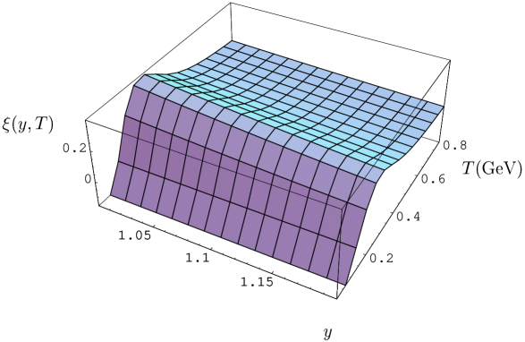
FIG. 2.:

FIG. 3.: