IFT-30/2000 December, 2000

We consider a general two-Higgs-doublet model with CP violation in the scalar sector. Three neutral Higgs fields of the model all mix and the resulting physical Higgs bosons have no definite CP properties. That leads, at the one-loop level of the perturbation expansion, to CP-violating form factors for $\gamma t\bar{t}$, $Zt\bar{t}$ and $Wtb$ interaction vertices. We discuss asymmetries sensitive to CP violation induced by the form factors for the process $e^{+}e^{-}\to t\bar{t}\to l^{\pm}\cdots$ and $e^{+}e^{-}\to t\bar{t}\to\stackrel{{\scriptstyle{\scriptscriptstyle(-)}}}{{b}}\cdots$ at future linear $e^{+}e^{-}$ colliders.

1 Introduction

Even though the top quark has been already discovered several years ago [1, *Abachi:1995iq], its interactions are still weakly constrained. It remains an open question if top-quark couplings obey the Standard Model (SM) scheme of the electroweak forces or there exists a contribution from physics beyond the SM. In particular, CP violation in the top-quark interactions has not been verified. The classical method for incorporating CP violation into the SM is to make the Yukawa couplings of the Higgs boson to quarks explicitly complex, as built into the Kobayashi-Maskawa mixing matrix [3] proposed more than two decades ago. However, CP violation could equally well be partially or wholly due to other mechanisms. The possibility that CP violation derives largely from the Higgs sector itself is particularly appealing in the context of the observed baryon asymmetry, since its explanation requires more CP violation [4, *Huet:1995jb] then is provided by the SM. Even the simple two-Higgs-doublet model (2HDM) extension of the one-doublet SM Higgs sector provides a much richer framework for describing CP violation; in the 2HDM, spontaneous and/or explicit CP violation is possible in the scalar sector [6, *Weinberg:1990me, *Branco:1985aq]. The model, besides CP violation, offers many other appealing phenomena, for a review see Ref. [9].

For our analysis, the most relevant part of the interaction Lagrangian takes the following form :

$${\cal{L}}=-\frac{m_{t}}{v}h\bar{t}(a+i\gamma_{5}b)t+C\frac{h}{v}(m_{Z}^{2}Z_{\mu}Z^{\mu}+2m_{W}^{2}W_{\mu}W^{\mu}),$$ (1)

where $h$ is the lowest mass scalar, $g$ is the SU(2) coupling constant, $v$ is the Higgs boson vacuum expectation value (with the normalization adopted here such that $v=2m_{W}/g=246\,\,{\rm GeV}$), $a$, $b$ and $C$ are real parameters which account for deviations from the SM, $a=1$, $b=0$ and $C=1$ reproduce the SM Lagrangian. Since under CP, $\bar{t}(a+i\gamma_{5}b)t\stackrel{{\scriptstyle{\rm CP}}}{{\rightarrow}}\bar{t}(a-i\gamma_{5}b)t$ and $Z_{\mu}Z^{\mu}\stackrel{{\scriptstyle{\rm CP}}}{{\rightarrow}}Z^{\mu}Z_{\mu}$, one can observe that terms in the cross section proportional to $ab$ or $bC$ would indicate CP violation. The 2HDM is the minimal extension of the SM that provides non-zero $ab$ and/or $bC$.

In this paper we will focus on CP-violating contributions to the process $e^{+}e^{-}\to t\bar{t}\to l^{\pm}\cdots$ and $e^{+}e^{-}\to t\bar{t}\to\stackrel{{\scriptstyle{\scriptscriptstyle(-)}}}{{b}}\cdots$ induced within 2HDM. However the fundamental goal is seeking for the ultimate theory of electroweak interactions. There are several reasons to utilize CP violation in the top physics while looking for physics beyond the SM:

• The top quark decays immediately after being produced as its huge mass $m_{t}=174.0\pm 3.2\pm 4.0\,{\rm GeV}$ [11] leads to a decay width ${\mit\Gamma}_{t}$ much larger than ${\mit\Lambda}_{\rm QCD}$. Therefore the decay process is not contaminated by any fragmentation effects [12, *Kuhn:1982ua, *Bigi:1986jk] and decay products may provide useful information on top-quark properties.

• Since the top quark is heavy, its Yukawa coupling is large and therefore its interactions could be sensitive to a Higgs sector of the electroweak theory.

• At the same time, the TESLA collider design is supposed to offer an integrated luminosity of the order of $L=500\;{\hbox{fb}^{-1}}{\hbox{y}^{-1}}$ at $\sqrt{s}=500\,{\rm GeV}$. Therefore expected number of $t\bar{t}$ events per year could reach $5\times 10^{4}$ even for $t\bar{t}$ tagging efficiency $\epsilon_{t\bar{t}}=15\%$. That should allow to study subtle properties of the top quark, which could e.g. lead to CP-sensitive asymmetries of the order of $5\times 10^{-3}$.

• Since the top quark is that heavy and the third family of quarks effectively decouples from the first two, any CP-violating observables within the SM are expected to be tiny, e.g.: i) non-zero electric dipole moment of fermions is generated at the three-loop approximation of the perturbation expansion [15], or ii) the decay rate asymmetry (being a one-loop effect) is strongly GIM suppressed reaching at most a value $10^{-9}$ [16]. So, one can expect that for CP-violating asymmetries any SM background could be safely neglected.

Therefore it seems to be justified to look for CP-violating Higgs effects in the process of $t\bar{t}$ production and its subsequent decay at future linear $e^{+}e^{-}$ colliders. Even though 2HDM contributions to various CP-sensitive asymmetries has been already presented in the existing literature, see Refs. [17, *Bernreuther:1992dz, 19], here we are providing a consistent treatment of CP violation both in the production, $e^{+}e^{-}\to t\bar{t}$, and in the top-quark decay, $t\to bW$. For an extensive review of CP violation in top-quark interactions see Ref. [20].

The paper is organized as follows. In Section 2, we briefly outline the mechanism of CP violation in the 2HDM, introduce the mixing matrix for neutral scalars and derive necessary couplings. In section 3, we present results for CP-violating form factors both for the $t\bar{t}$ production process and for $t$ and $\bar{t}$ decays. In Section 4, we recall current experimental constraints relevant for the CP-violating observables considered in this paper. In Section 5, we collect results for various energy and angular CP-violating asymmetries. Concluding remarks are given in Section 6.

2 The two-Higgs-doublet model with CP violation

The 2HDM of electroweak interactions contains two SU(2) Higgs doublets denoted by $\Phi_{1}=(\phi_{1}^{+},\phi_{1}^{0})$ and $\Phi_{2}=(\phi_{2}^{+},\phi_{2}^{0})$. It is well known [6, *Weinberg:1990me, *Branco:1985aq] that the model allows both for spontaneous and explicit CP violation.

After SU(2)$\times$U(1) gauge symmetry breaking, one combination of neutral Higgs fields, $\sqrt{2}(c_{\beta}\Im\phi_{1}^{0}+s_{\beta}\Im\phi_{2}^{0})$, becomes a would-be Goldstone boson which is absorbed while giving mass to the $Z$ gauge boson. (Here, we use the notation $s_{\beta}\equiv\sin\beta$, $c_{\beta}\equiv\cos\beta$, where $\tan\beta=\langle\phi_{2}^{0}\rangle/\langle\phi_{1}^{0}\rangle$.) The same mixing angle, $\beta$, also diagonalizes the mass matrix in the charged Higgs sector. If either explicit or spontaneous CP violation is present, the remaining three neutral degrees of freedom,

$$(\varphi_{1},\varphi_{2},\varphi_{3})\equiv\sqrt{2}(\Re\phi_{1}^{0},\,\Re\phi_{2}^{0},\,s_{\beta}\Im\phi_{1}^{0}-c_{\beta}\Im\phi_{2}^{0})$$ (2)

are not mass eigenstates. The physical neutral Higgs bosons $h_{i}$ ($i=1,2,3$) are obtained by an orthogonal transformation, $h=R\varphi$, where the rotation matrix is given in terms of three Euler angles ($\alpha_{1},\alpha_{2},\alpha_{3}$) by

$$R=\left(\begin{array}[]{ccc}c_{1}&-s_{1}c_{2}&s_{1}s_{2}\\ s_{1}c_{3}&c_{1}c_{2}c_{3}-s_{2}s_{3}&-c_{1}s_{2}c_{3}-c_{2}s_{3}\\ s_{1}s_{3}&c_{1}c_{2}s_{3}+s_{2}c_{3}&-c_{1}s_{2}s_{3}+c_{2}c_{3}\end{array}\right),$$ (6)

where $s_{i}\equiv\sin\alpha_{i}$ and $c_{i}\equiv\cos\alpha_{i}$.

As a result of the mixing between real and imaginary parts of neutral Higgs fields, the Yukawa interactions of the $h_{i}$ mass-eigenstates are not invariant under CP. They are given by:

$${\cal L}=-\frac{m_{f}}{v}h_{i}\bar{f}(a^{f}_{i}+ib^{f}_{i}\gamma_{5})f$$ (7)

where the scalar ($a^{f}_{i}$) and pseudoscalar ($b^{f}_{i}$) couplings are functions of the mixing angles. For up-type quarks we have

$$a^{u}_{i}=\frac{1}{s_{\beta}}R_{i2},\;\;\;\;\;b^{u}_{i}=\frac{c_{\beta}}{s_{\beta}}R_{i3},$$ (8)

and for down-type quarks:

$$a^{d}_{i}=\frac{1}{c_{\beta}}R_{i1},\;\;\;\;\;b^{d}_{i}=\frac{s_{\beta}}{c_{\beta}}R_{i3}\,,$$ (9)

and similarly for charged leptons. For large $\tan\beta$, the couplings to down-type fermions are typically enhanced over the couplings to up-type fermions.

In the following analysis we will also need the couplings of neutral Higgs and vector bosons, they are given by

$$g_{VVh_{i}}\equiv 2\frac{m_{V}^{2}}{v}C_{i}=2\frac{m_{V}^{2}}{v}(s_{\beta}R_{i2}+c_{\beta}R_{i1}),$$ (10)

for $V=Z,W$. Hereafter we shall denote the lightest Higgs boson by $h$ and its $R$-matrix index by $i$.

3 Form Factors

3.1 $t\bar{t}$ Production

Figure 1: Diagrams contributing to CP-violating form factors $D_{\gamma,Z}$.

The effective $t\bar{t}\gamma$ and $t\bar{t}Z$ vertices will be parameterized by the following form factors:

$${\mit\Gamma}^{\mu}_{v}=\frac{g}{2}\bar{u}(p_{t})\biggl{[}\,\gamma^{\mu}(A_{v}-B_{v}\gamma_{5})+\frac{(p_{t}-p_{\bar{t}})^{\mu}}{2m_{t}}(C_{v}-D_{v}\gamma_{5})\,\biggr{]}v(p_{\bar{t}}),$$ (11)

where $g$ denotes the SU(2) gauge coupling constant, $v=\gamma,Z$, and

$$A_{\gamma}=-\frac{4}{3}\sin\theta_{W},\ \ B_{\gamma}=0,\ \ A_{Z}=-\frac{v_{t}}{2\cos\theta_{W}},\ \ B_{Z}=-\frac{a_{t}}{2\cos\theta_{W}},\ \ C/D_{\gamma,Z}=0$$

denote the SM contributions to the vertices for

$$v_{t}=\Bigl{(}1-\frac{8}{3}\sin^{2}\theta_{W}\Bigr{)}\;\;\;\;\;\;\;\;a_{t}=1.$$

The form factors $A_{v}$, $B_{v}$, $C_{v}$ describe $CP$-conserving while $D_{v}$ parameterizes $CP$-violating contributions.

Further in this paper the following parameters will be adopted: $m_{t}=175\,{\rm GeV}$, $m_{Z}=91.187\,{\rm GeV}$, $\Gamma_{Z}=2.49\,{\rm GeV}$, $\sin^{2}\theta_{W}=0.23$ and $m_{b}=4.2\,{\rm GeV}$.

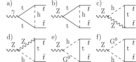
Since in this paper we are focusing on CP-violating asymmetries, the only relevant form factors are $D_{\gamma}$ and $D_{Z}$. Direct calculation of diagrams shown in Fig.1 leads to the following result in terms of 3-point Passarino-Veltman [21] functions defined in the appendix A.1:

$$D_{\gamma} = \frac{\mathrm{i}\mkern 1.0mu}{2\pi^{2}}A_{\gamma}\frac{m_{t}^{2}}{v^{2}}b_{i}^{t}a_{i}^{t}m_{t}^{2}{\mathbf{C}}_{12}(p_{t},p_{\bar{t}},m_{t}^{2},m_{h}^{2},m_{t}^{2}),$$

$$D_{Z} = \frac{\mathrm{i}\mkern 1.0mu}{2\pi^{2}}A_{Z}\frac{m_{t}^{2}}{v^{2}}b_{i}^{t}\left[a_{i}^{t}m_{t}^{2}{\mathbf{C}}_{12}(p_{t},p_{\bar{t}},m_{t}^{2},m_{h}^{2},m_{t}^{2})\right.$$ (12)

$$\left.-C_{i}m_{Z}^{2}{\mathbf{C}}_{12}(p_{t},p_{\bar{t}},m_{h}^{2},m_{t}^{2},m_{Z}^{2})\right].$$

Since the asymmetries we are going to discuss are generated by real parts of the above form factors, let us decompose (using eqs.(8, 10)) $\Re(D_{\gamma})$ and $\Re(D_{Z})$ in the following way:

$$\Re D_{\gamma} = R_{i2}R_{i3}f_{23}^{\gamma(a)}$$ (13)

$$\Re D_{Z} = R_{i2}R_{i3}(f_{23}^{Z(b)}+f_{23}^{Z(c-f)})+R_{i1}R_{i3}f_{13}^{Z(c-f)},$$

where superscripts indicate graphs that generate the contribution according to the notation of Fig.1. Since in the case of the photon only Yukawa couplings $a_{i}^{t}$ and $b_{i}^{t}$ contribute, any signal of CP violation must be proportional to $a_{i}^{t}b_{i}^{t}\sim R_{i2}R_{i3}$. However, for the $Z$ boson vertex there is also other “source” of CP violation, namely $b_{i}^{t}C_{i}\ni R_{i1}R_{i3}$.

It is useful to discuss $\tan\beta$ dependence of the functions $f$ first. From eq.(3.1) and eqs.(8, 10) one can find out that all contributions to the form factors $D_{\gamma}$, $D_{Z}$ are enhanced for small $\tan\beta$: $f_{23}^{\gamma(a)},\;f_{23}^{Z(b)}\sim\tan^{-2}\beta$, $f_{23}^{Z(c-f)}\sim\cos\beta$ and $f_{13}^{Z(c-f)}\sim\tan^{-1}\beta$. Therefore, for $\tan\beta<1$, the contributions from diagrams c)-f) are expected to be suppressed relatively to those generated by diagrams a) or b) in Fig.1.

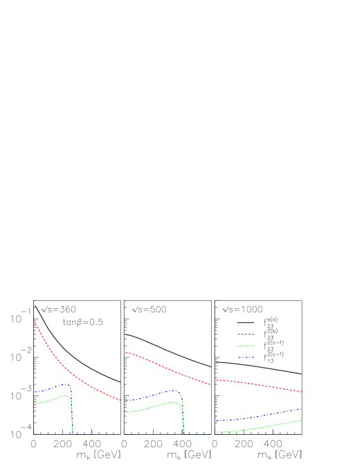
Hereafter we assume that there exists only one light Higgs boson $h$ and possible effects of the heavier scalar degrees of freedom decouple. In Fig.2 we illustrate dependence of the functions $f$ on the lightest Higgs boson mass, $m_{h}$. In order to amplify possible contributions we have chosen $\tan\beta=0.5$. As it is seen from the figure, the dominant CP-violating effects will be generated by $f_{23}^{\gamma(a)}$ and $f_{23}^{Z(b)}$, which are generated by the Yukawa-coupling contribution, $a_{i}^{t}b_{i}^{t}$, from diagrams a) and b) in Fig.1. As one could have anticipated, we observe an enhancement of the contributions generated by the diagrams a) and b) for low Higgs boson mass. The growth of $f_{23}^{\gamma(a)}$ and $f_{23}^{Z(b)}$ is more pronounced for lower $\sqrt{s}$ (closer to the $t\bar{t}$ production threshold), it is a consequence of the Coulomb-like singularity generated by graph a) and b) in the limit $m_{h}\to 0$ at the $t\bar{t}$ production threshold. Similar behavior have been also noted in the case of CP-conserving form factors [22]. One also observes a typical threshold behavior at $(\sqrt{s}-m_{Z})$ for $f_{23}^{Z(c-f)}$ and $f_{13}^{Z(c-f)}$ as a non-trivial absorptive part of diagrams c)-f) is necessary for nonzero contribution to $\Re D_{Z}$.

If all three Higgs bosons of the model have the same mass, then the orthogonality of the mixing matrix $R_{ij}$ guarantees [23] vanishing CP violation while summed over all the scalars. Therefore, the leading contribution to $\Re D_{\gamma}$ and $\Re D_{Z}$ originating from an exchange of the lightest Higgs boson $h$ could be partially cancelled by heavier scalars $h_{h}$. However here we will assume that masses of the heavier scalars are above the production threshold for $Zh_{h}$, therefore, as observed (for the lightest Higgs boson mass below $100\,{\rm GeV}$) from Fig.2, the cancellation by heavier scalars for $\sqrt{s}=360,\;,500$ and $1000\,{\rm GeV}$ could reach at most $20,\;30$ and $40\%$.

Leading asymptotic formulae for small and large Higgs mass are presented in the appendix A.2. It is worth to notice that for non-zero $\beta_{t}=\sqrt{1-4m_{t}^{2}/s}$, in the limit $m_{h}^{2}/(\beta^{2}_{t}s)\to 0$ both $\Re D_{\gamma}$ and $\Re D_{Z}$ are finite, whereas a typical decoupling limit, $\Re D_{\gamma},\Re D_{Z}\sim m_{t}^{4}/(m_{h}^{2}m_{W}^{2})$, is observed for large $m_{h}$.

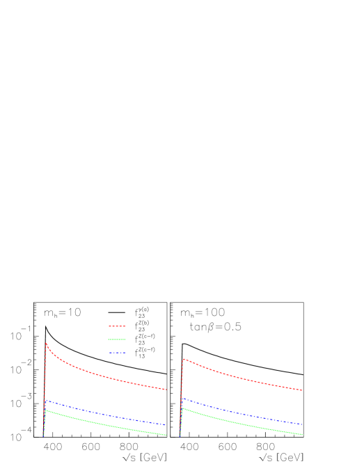
Fig.3 shows the functions $f$ for $\tan\beta=0.5$ and two different Higgs boson masses $m_{h}=10\,{\rm GeV}$ and $m_{h}=100\,{\rm GeV}$, as a function of $\sqrt{s}$. It is seen that it is not desirable to choose too high beam energy, as the size of the functions drops. Again, $f_{23}^{\gamma(a)},\;f_{23}^{Z(b)}$ dominate over $f_{13}^{Z(c-f)},\;f_{23}^{Z(c-f)}$ by 1-2 orders of magnitude.

Figure 2: The functions $f$ defined in eq. (3.1) as a function of $m_{h}$ for $\tan\beta=0.5$, $\sqrt{s}=360$ (left), $\sqrt{s}=500$ (middle) and $\sqrt{s}=1000\,{\rm GeV}$ (right).

Figure 3: The functions $f$ defined in eq. (3.1) as a function of $\sqrt{s}$ for $\tan\beta=0.5$, $m_{h}=10\,{\rm GeV}$ and $m_{h}=100\,{\rm GeV}$

3.2 Top Decay

We will adopt the following parameterization of the $Wtb$ vertex suitable for the $t$ and $\bar{t}$ decays:

$${\Gamma}^{\mu} = -\frac{g}{\sqrt{2}}V_{tb}\>\biggl{[}\,\gamma^{\mu}(f_{1}^{L}P_{L}+f_{1}^{R}P_{R})-\frac{{i\sigma^{\mu\nu}k_{\nu}}}{M_{W}}(f_{2}^{L}P_{L}+f_{2}^{R}P_{R})\,\biggr{]},\ \ \ \$$

$$\bar{\Gamma}^{\mu} = -\frac{g}{\sqrt{2}}V_{tb}^{*}\>\biggl{[}\,\gamma^{\mu}(\bar{f}_{1}^{L}P_{L}+\bar{f}_{1}^{R}P_{R})-\frac{{i\sigma^{\mu\nu}k_{\nu}}}{M_{W}}(\bar{f}_{2}^{L}P_{L}+\bar{f}_{2}^{R}P_{R})\,\biggr{]},$$ (14)

where $P_{L/R}=(1\mp\gamma_{5})/2$, $V_{tb}$ is the $(tb)$ element of the Kobayashi-Maskawa matrix and $k$ is the momentum of $W$. In the SM $f_{1}^{L}=\bar{f}_{1}^{L}=1$ and all the other form factors vanish. It turns out that in the limit of massless bottom quarks the only form factors that interfere with the SM are $f_{2}^{R}$ and $\bar{f}_{2}^{L}$ for the top and anti-top decays, respectively. Currently, there is no relevant experimental bound on those form factors.

One can show that the CP-violating and CP-conserving parts of the form factors for $t$ and $\bar{t}$ are not independent:

$$f_{1}^{L,R}=\pm\bar{f}_{1}^{L,R}\;\;{\rm and}\;\;\;f_{2}^{L,R}=\pm\bar{f}_{2}^{R,L},$$ (15)

where upper (lower) signs are those for $CP$-conserving (-violating) contributions [29, 19]. Therefore any $CP$-violating observable defined for the top-quark decay must be proportional to $f_{1}^{L,R}-\bar{f}_{1}^{L,R}$ or $f_{2}^{L,R}-\bar{f}_{2}^{R,L}$.

Figure 4: Diagrams contributing to $f_{2}^{R}-\bar{f}_{2}^{L}$.

Diagrams contributing to CP violation in the decay process are shown in Fig.4. Direct calculation leads to the following result for the CP-violating part of $f_{2}^{R}$ :

$$f_{2}^{R}|_{CPV}=\frac{\mathrm{i}\mkern 1.0mug}{32\pi^{2}}\frac{m_{b}}{v}m_{t}m_{b}\Big{\{}\left[2a_{i}^{b}b_{i}^{t}{\mathbf{C}}_{12}^{a}+\left(a_{i}^{b}b_{i}^{t}-a_{i}^{t}b_{i}^{b}\right){\mathbf{C}}_{23}^{a}\right]-b_{i}^{b}C_{i}{\mathbf{C}}_{22}^{bd}$$

$$+b_{i}^{t}C_{i}\left[{\mathbf{C}}_{22}^{ce}+{\mathbf{C}}_{23}^{ce}\left(\frac{m_{t}^{2}}{m_{b}^{2}}-1\right)+2\left({\mathbf{C}}_{12}^{ce}-{\mathbf{C}}_{11}^{ce}\right)\frac{m_{W}^{2}}{m_{b}^{2}}\right]$$ (16)

$$+\left[2a_{i}^{b}C^{2}_{i}{\mathbf{C}}_{12}^{f}ct_{\beta}-{\mathbf{C}}_{22}^{f}\Im(y_{i}^{b}C^{-}_{i})t_{\beta}+{\mathbf{C}}_{23}^{f}\left(\Im(y_{i}^{b}C^{+}_{i})ct_{\beta}+\Im(y_{i}^{b}C^{-}_{i})t_{\beta}\right)\right]$$

$$\left.-\left[2a_{i}^{t}C^{2}_{i}{\mathbf{C}}_{12}^{g}ct_{\beta}\frac{m_{t}^{2}}{m_{b}^{2}}-{\mathbf{C}}_{22}^{g}\Im(y_{i}^{t}C^{-}_{i})t_{\beta}+{\mathbf{C}}_{23}^{g}\left(\Im(y_{i}^{t}C^{+}_{i})\frac{m_{t}^{2}}{m_{b}^{2}}ct_{\beta}+\Im(y_{i}^{t}C^{-}_{i})t_{\beta}\right)\right]\right\}$$

where

$${\mathbf{C}}_{ij}^{a} = {\mathbf{C}}_{ij}(p_{t},-p_{W},m_{h}^{2},m_{t}^{2},m_{b}^{2})$$

$${\mathbf{C}}_{ij}^{bd} = {\mathbf{C}}_{ij}(p_{W},p_{b},m_{W}^{2},m_{h}^{2},m_{b}^{2})$$

$${\mathbf{C}}_{ij}^{ce} = {\mathbf{C}}_{ij}(p_{W},p_{b},m_{h}^{2},m_{W}^{2},m_{t}^{2})$$

$${\mathbf{C}}_{ij}^{f} = {\mathbf{C}}_{ij}(p_{W},-p_{t},m_{h}^{2},m_{H}^{2},m_{b}^{2})$$

$${\mathbf{C}}_{ij}^{g} = {\mathbf{C}}_{ij}(p_{W},p_{b},m_{h}^{2},m_{H}^{2},m_{t}^{2})$$ (17)

and

$$y_{i}^{t/b}\equiv a_{i}^{t/b}+\mathrm{i}\mkern 1.0mub_{i}^{t/b},\ \ \ C_{i}^{\pm}\equiv C_{i}^{(1)}\pm\mathrm{i}\mkern 1.0muC_{i}^{(2)},\ \ \ t_{\beta}=\tan\beta,\ \ ct_{\beta}=\cot\beta,$$ (18)

where $C_{i}^{(1)}=s_{\beta}R_{i1}-c_{\beta}R_{i2}$ and $C_{i}^{(2)}=R_{i3}$. The asymmetries that will be discussed here depends on real parts of $f_{2}^{R}$ and $\bar{f}_{2}^{L}$. It is easy to note from eq.(3.2) that imaginary parts of ${\mathbf{C}}$ functions contribute to the real part of $f_{2}^{R}|_{CPV}$. It is seen that only diagrams b), d) and f) will contribute to $\Re(f_{2}^{R}|_{CPV})$. However, $b\rightarrow s\gamma$ strongly suggest [30] that for 2HDM $m_{H^{\pm}}>m_{t}-m_{b}$, therefore eventually (adopting the relation (15)) one gets the following result (from graphs b) and d) only) for CP-violating contribution to $\Re(f_{2}^{R}|_{CPV})$:

$$\Re(f_{2}^{R}-\bar{f}_{2}^{L})=2\Re(f_{2}^{R}|_{CPV})=\frac{g}{16\pi^{2}}\frac{m_{b}}{v}m_{b}m_{t}b_{i}^{b}C_{i}\Im{\mathbf{C}}_{22}^{bd}$$ (19)

As will be discussed in Section 4 there is a strong experimental bound on $|C_{i}|$ for $m_{h}<105\,{\rm GeV}$. Taking into account the limit on $|C_{i}|$ and choosing $\tan\beta=50$ (in order to illustrate a possible enhancement) we plot $\Re(f_{2}^{R}-\bar{f}_{2}^{L})$ in Fig. 4 as a function of $m_{h}$. It is seen that $\Re(f_{2}^{R}-\bar{f}_{2}^{L})$ is by $2-4$ orders of magnitude below $\Re D_{\gamma}$ or $\Re D_{Z}$ even for large b-quark Yukawa coupling, compare Fig. 2 and 3. The suppression is caused both by the experimental limit on $|C_{i}|$ (for $m_{h}<105\,{\rm GeV}$) and by an extra suppression factor of $(m_{b}/m_{t})^{2}$ (relative to $\Re D_{\gamma,Z}$).

There is a comment in order here; since in the 2HDM the real part of CP-violating form factors in the top decay is much smaller then in the production process, it is interesting to look closer at the suppression mechanism and find class of possible extensions of the SM that provide large $\Re(f_{2}^{R}-\bar{f}_{2}^{L})$. Since an absorptive part is needed, the only graphs that may contribute are those denoted by b), d) and f) in Fig.4 (allowing for the neutral scalar to be replaced by a neutral vector). One source of the suppression is the bottom-quark mass that originate from the propagator while the second one comes from the Yukawa vertex. The latter one could be easy amplified by large $\tan\beta$: for $\tan\beta\simeq 38$ the bottom-quark Yukawa coupling is as strong as the SU(2) gauge coupling. Therefore the suppression to overcome is $m_{b}$ from the bottom-quark propagator. A possible solution [31] seems to be a multi-doublet-Higgs model that could evade the stringent restriction from the $b\to s\gamma$ decay and also overcome (through a contribution from the graph type f) in Fig.4) the limit on $W^{+}W^{-}h$ that comes from the LEP limit on $|C_{i}|$. Let us notice that it is much easier to develop large $\Im(f_{2}^{R}-\bar{f}_{2}^{L})$, see e.g. Refs. [19] and [20].

Figure 5: $\Re(f_{2}^{R}-\bar{f}_{2}^{L})$ as a function of $m_{h}$ for $\tan\beta=50$. It has been assumed (according to constraints from $b\to s\gamma$) that the charged Higgs boson is heavy, $m_{H^{\pm}}>m_{t}-m_{b}$, therefore there is no absorptive part necessary to develop a non-zero contribution from diagram f) in Fig.4. Additionally, we assumed $C_{i}=R_{i2}$ (what is a very good approximation for $\tan\beta=50$) and selected such values for $R_{i2}$ and $R_{i3}$ that are consistent both with $R_{ij}$ orthogonality and $C_{i}$ LEP bound, and provide a maximal value of $\Re(f_{2}^{R}-\bar{f}_{2}^{L})$.

It is worth to mention that even though in the SM there exists one-loop contribution to $\Re(f_{2}^{R}-\bar{f}_{2}^{L})$, it turns out to be strongly GIM suppressed [16]. Therefore, although the 2HDM prediction for $\Re(f_{2}^{R}-\bar{f}_{2}^{L})$ is smaller than for CP violating from factors in the production mechanism, it is still by a factor $\sim 10^{5}$ larger then the SM result.

4 Experimental Constraints

Hereafter we will focus on Higgs boson masses in the region, $m_{h}=10\div 100\,{\rm GeV}$. As it has been shown in the literature [32, *Abreu:2000kg, *Abbiendi:2000ug] the existing LEP data are perfectly consistent with one light Higgs boson within the 2HDM. It turns out that even precision electroweak tests allow for light Higgs bosons [35].

In order to amplify the form factors calculated in this paper we have adopted for an illustration $\tan\beta=0.5$. However, there exist experimental constraints on $\tan\beta$ from ${\rm K^{0}-\bar{K}^{0}}$ and ${\rm B_{d}-\bar{B}_{d}}$ mixing [36], $b\to s\gamma$ decay [30] and $Z\to b\bar{b}$ decay [37]. Since small $\tan\beta$ enhances $H^{\pm}tb$ coupling, in order to maintain $\tan\beta=0.5$ we have to decouple charged Higgs effects and therefore we assume that $m_{H^{\pm}}\mathrel{\raise 1.29167pt\hbox{$>$\kern-7.5pt\lower 4.30554pt\hbox{$\sim$}}}500\div 600\,{\rm GeV}$.

The constraints on the mixing angles $\alpha_{i}$ that should be imposed in our numerical analysis are as follows:

• The $ZZh$ couplings, $C_{i}^{2}$, are restricted by non-observation of Higgs-strahlung events at LEP1 and LEP2, see Ref. [38, *ALEPH2000-028]

• The contribution to the total $Z$-width from $Z\rightarrow Z^{*}h_{i}\rightarrow f\bar{f}h_{i}$ is required to be below $7.1\,{\rm MeV}$, see Ref. [40].

It turns out that the restriction on the $ZZh$ coupling from its contribution to the total $Z$-width is always weaker then the one from $Zh$ production if $m_{h}\mathrel{\raise 1.29167pt\hbox{$>$\kern-7.5pt\lower 4.30554pt\hbox{$\sim$}}}10\,{\rm GeV}$.

The LEP constraints on the $ZZh$ coupling restrict the following entries of the mixing matrix $R_{ij}$:

$$|\sin\beta R_{i2}+\cos_{\beta}R_{i1}|\leq C_{i}^{exp},$$ (20)

where $C_{i}^{exp}$ stands for the upper limit for the relative strength of $ZZh$ coupling determined experimentally in Ref. [38, *ALEPH2000-028] up to the Higgs mass $m_{h}=105\,{\rm GeV}$. As we have concluded in the previous section, CP-violating phenomena we are considering are enhanced by small $\tan\beta$, in that case one can see from eq.(20) that the LEP constraints mostly restrict $R_{i1}$. Through the orthogonality the restriction on $R_{i1}$ is being transfered to constrain $|R_{i2}R_{i3}|=|R_{i2}\sqrt{1-R_{i1}^{2}-R_{i2}^{2}}|$ which multiplies leading contributions to all CP-violating asymmetries considered here. The final result for upper limit on $|R_{i2}R_{i3}|$ as a function of $\tan\beta$ is shown in Fig.6. In fact the bound on $|R_{i2}R_{i3}|$ depends on the Higgs mass, however, in order to be conservative, we have assumed $C_{i}^{exp}=0.12$ that is the most restrictive experimental limit (obtained for $m_{h}\simeq 18\,{\rm GeV}$).

Figure 6: Maximal value of $|R_{i2}R_{i3}|$ allowed by the LEP constraints on $ZZh_{i}$ coupling as a function of $\tan\beta$.

As it is seen from Fig.6 the constraints for $|R_{i2}R_{i3}|$ are weak for small $\tan\beta$. Therefore for $\tan\beta\simeq 0.5$ it should be legitimate to assume $|R_{i2}R_{i3}|\simeq 1/2$ which is the maximal value consistent with orthogonality.

Using the maximal value of $R_{i2}R_{i3}$ allowed by the orthogonality and the LEP constraints for small $\tan\beta=0.5$, we may discuss a possibility for an experimental determination of the calculated form factors at future $e^{+}e^{-}$ colliders. A detailed discussion of expected statistical uncertainties for a measurement of the form factors has been performed in Ref. [41]. It has been shown that adjusting an optimal $e^{+}e^{-}$ beam polarizations, using the energy and angular double distribution of final leptons and fitting all 9 form factors leads to the following statistical errors for the determination of CP-violating form factors: $\Delta[\Re(D_{\gamma})]=0.08$ and $\Delta[\Re(D_{Z})]=14.4$ for $\epsilon_{t\bar{t}}\simeq 15\%$. It is seen that only $\Re(D_{\gamma})$, could be measured with a high precision. We have observed in Figs.2,3 that $\Re(D_{\gamma})$ may reach at most a value of $0.10$, therefore one shall conclude that several years of running with yearly integrated luminosity $L=500\;{\hbox{fb}^{-1}}{\hbox{y}^{-1}}$ should allow for an observation of $\Re(D_{\gamma})$ generated within 2HDM, provided the lightest Higgs boson mass is not too large. On the other hand, the expected [41] precision for the determination of the decay form factors is much more promising: $\Delta[\Re(f_{2}^{R}-\bar{f}_{2}^{L})]=0.014$. However, as we have seen in Fig.5, the maximal expected size of $\Re(f_{2}^{R}-\bar{f}_{2}^{L})$ is $5\times 10^{-5}$ (for $m_{h}>10\,{\rm GeV}$), therefore either an unrealistic growth of the luminosity, or other observables (besides the energy and angular double distribution of final leptons) are required in order to observe CP-violating from factors in the top-quark decay process. The results of Ref. [41] assumed simultaneous determination of all 9 form factors, therefore another chance to reduce of $\Delta[\Re(f_{2}^{R}-\bar{f}_{2}^{L})]$ is to have some extra independent constraints on the top-quark coupling coming from other colliders, like the Fermilab Tevatron or LHC.

5 CP-Violating Asymmetries

Looking for CP violation one can directly measure [41] all the form factors including those which are odd under CP. However another possible attitude is to construct certain asymmetries sensitive to CP violation. In this section we will discuss several asymmetries that could probe CP violation in the process $e^{+}e^{-}\to t\bar{t}\to l^{\pm}\cdots$. We will systematically drop all contributions quadratic in non-standard form factors and calculate various asymmetries keeping only interference between the SM and $D_{\gamma}$, $D_{Z}$ or $\Re(f_{2}^{R}-\bar{f}_{2}^{L})$.

5.1 Lepton-Energy Asymmetry

Let us introduce the rescaled lepton energy, $x$, by

$$x\equiv\frac{2E_{l}}{m_{t}}\left(\frac{1-\beta_{t}}{1+\beta_{t}}\right)^{1/2},$$ (21)

where $E_{l}$ is the energy of $l$ in $e^{+}e^{-}$ c.m. frame and $\beta_{t}\equiv\sqrt{1-4m_{t}^{2}/s}$. Using lepton energy distribution $d\sigma^{\pm}/dx$ calculated [42] for the general form factors given in eqs.(11,14) one can define the following energy asymmetry:

$${\cal A}_{CP}^{l}(x)\equiv\frac{d\sigma^{-}/dx-d\sigma^{+}/dx}{d\sigma^{-}/dx+d\sigma^{+}/dx}$$ (22)

Direct calculation leads to the following result in terms of the CP-violating form factors:

$${\cal A}_{CP}^{l}(x)=\frac{2\xi g(x)+\Re{(f_{2}^{R}-\bar{f}_{2}^{L})}[\,\delta\!f(x)+\eta\>\delta g(x)\,]}{2\,[\,f(x)+\eta\>g(x)\,]}.$$ (23)

where

$$\xi\equiv\frac{1}{(3-\beta^{2})D_{V}+2\beta^{2}D_{A}}$$

$$\ \ \ \ \ \times\frac{-1}{\sin\theta_{W}}{\Re}\biggl{[}\>\frac{2}{3}\>D_{\gamma}+\frac{s^{2}}{(s-m_{Z}^{2})^{2}}\frac{(v_{e}^{2}+a_{e}^{2})v_{t}}{64\sin^{3}\theta_{W}\cos^{3}\theta_{W}}D_{Z}$$

$$\ \ \ \ \ -\frac{s}{s-m_{Z}^{2}}\biggl{(}\,\frac{v_{e}v_{t}}{16\sin^{2}\theta_{W}\cos^{2}\theta_{W}}D_{\gamma}+\frac{v_{e}}{6\sin\theta_{W}\cos\theta_{W}}D_{Z}\,\biggr{)}\>\biggr{]},$$

for

$$D_{V}=(v_{e}v_{t}d-\frac{2}{3})^{2}+(a_{e}v_{t}d)^{2},$$

$$D_{A}=(v_{e}a_{t}d)^{2}+(a_{e}a_{t}d)^{2},$$

with the SM neutral-current parameters of $e$ and $t$: $v_{e}=-1+4\sin^{2}\theta_{W}$, $a_{e}=-1$, $v_{t}=1-(8/3)\sin^{2}\theta_{W}$, and $a_{t}=1$, and a $Z$-propagator factor

$$d\equiv\frac{s}{s-m_{Z}^{2}}\frac{1}{16\sin^{2}\theta_{W}\cos^{2}\theta_{W}}.$$

The coefficient $\eta$ is defined as

$$\eta\equiv\frac{{4\>{\Re}(D_{V\!A})}}{{(3-\beta^{2})D_{V}+2\beta^{2}D_{A}}}.$$

for

$$D_{V\!A}=v_{e}a_{t}d(v_{e}v_{t}d-\frac{2}{3})+(a_{e}d)^{2}a_{t}v_{t}.$$

The definitions of the functions $f$, $g$, $\delta f$ and $\delta g$ could be obtained from Ref. [42].

Figure 7: The coefficient functions $g$ defined by eq.(24) for the energy-asymmetry as function of $x$ for $\sqrt{s}=$ 360 (left), 500 (middle) and 1000 GeV (right) for $\tan\beta=0.5$. The solid curve represents the coefficient $g_{\gamma t\bar{t}}^{l}(x)$, dashed $g_{Zt\bar{t}}^{l}(x)$ and dotted $g_{Wtb}^{l}(x)$.

In order to estimate a relative strength of various sources of CP violation it is worth to decompose the asymmetry as follows:

$${\cal A}_{CP}^{l}(x)=g_{\gamma t\bar{t}}^{l}(x)\ \Re D_{\gamma}+g_{Zt\bar{t}}^{l}(x)\ \Re D_{Z}+g_{Wtb}^{l}(x)\ \Re(f_{2}^{R}-\bar{f}_{2}^{L}).$$ (24)

As one can see from Fig.7 the CP-violating effects that originate from the decay are substantially enhanced in the soft energy region. It is worth to notice that the minimal lepton energy for $\sqrt{s}=500\,{\rm GeV}$ is $E_{l}^{min}\simeq 7.5\,{\rm GeV}$ that is large enough to detect the lepton. Therefore the region of soft leptons should be carefully studied experimentally. The enhancement is a consequence of particular behavior of $f(x)+\eta g(x)$, $g(x)$ and $\delta f(x)+\eta\delta g(x)$ that causes the relative amplification of the decay effects, see Fig.1 in Ref. [43]. The same figure explains the observed smallness of the $Z$-boson contribution. For hard leptons both $\Re(f_{2}^{R}-\bar{f}_{2}^{L})$ and $\Re D_{\gamma}$ are enhanced and they are raising with the c.m. energy.

The energy-asymmetry could be decomposed into the leading contribution proportional to $R_{i2}R_{i3}$ and the remaining piece proportional to $R_{i1}R_{i3}$. The former one (that provides the leading contribution) is plotted in Fig.8 for a fixed energy, $x=0.8$, as a function of $m_{h}$. One can observe that the largest asymmetry for the chosen energy corresponds to $\sqrt{s}=360\,{\rm GeV}$ and $m_{h}=10\,{\rm GeV}$.

Figure 8: The Higgs mass dependence of the coefficient of $R_{i2}R_{i3}$ for the asymmetry given by eq.(22) for $\sqrt{s}$=360 (solid), 500 (dashed), 1000 GeV (dotted) for a fixed energy, $x_{l}=0.8$, and $\tan\beta=0.5$.

5.2 Integrated Lepton-Energy Asymmetry

CP symmetry could be also tested using the following leptonic double energy distribution [44]:

$$\frac{1}{\sigma}\frac{d^{2}\sigma}{dx\;d\bar{x}}=\sum_{i=1}^{3}c_{i}f_{i}(x,\bar{x}),$$ (25)

where $x$ and $\bar{x}$ are for $l^{+}$ and $l^{-}$ respectively, for

$$c_{1}=1,\ \ \ c_{2}=\xi,\ \ \ c_{3}=\frac{1}{2}\Re(f_{2}^{R}-\bar{f}_{2}^{L})$$

and

$$f_{1}(x,\bar{x})=f(x)f(\bar{x})+\eta^{\prime}g(x)g(\bar{x})+\eta[f(x)g(\bar{x})+g(x)f(\bar{x})],$$

$$f_{2}(x,\bar{x})=f(x)g(\bar{x})-g(x)f(\bar{x}),$$

$$f_{3}(x,\bar{x})=\delta\!f(x)f(\bar{x})-f(x)\delta\!f(\bar{x})+\eta^{\prime}[\delta g(x)g(\bar{x})-g(x)\delta g(\bar{x})]$$

$$\ \ \ \ \ \ \ \ \ \ \ +\eta[\delta\!f(x)g(\bar{x})-f(x)\delta g(\bar{x})+\delta g(x)f(\bar{x})-g(x)\delta\!f(\bar{x})],$$

where

$$\eta^{\prime}\equiv\frac{1}{\beta^{2}}\frac{(1+\beta^{2})D_{V}+2\beta^{2}D_{A}}{(3-\beta^{2})D_{V}+2\beta^{2}D_{A}}.$$

The following asymmetry could be a measure of CP violation:

$$A_{CP}^{ll}\equiv\frac{\displaystyle\int\int_{x<\bar{x}}dxd\bar{x}\frac{d^{2}\sigma}{\displaystyle dxd\bar{x}}-\int\int_{x>\bar{x}}dxd\bar{x}\frac{d^{2}\sigma}{\displaystyle dxd\bar{x}}}{\displaystyle\int\int_{x<\bar{x}}dxd\bar{x}\frac{d^{2}\sigma}{\displaystyle dxd\bar{x}}+\int\int_{x>\bar{x}}dxd\bar{x}\frac{d^{2}\sigma}{\displaystyle dxd\bar{x}}}.$$ (26)

As before, it is useful to separate contributions from various form factors:

$$A_{CP}^{ll}=g_{\gamma t\bar{t}}^{ll}\ \Re D_{\gamma}+g_{Zt\bar{t}}^{ll}\ \Re D_{Z}+g_{Wtb}^{ll}\ \Re(f_{2}^{R}-\bar{f}_{2}^{L}).$$ (27)

In Table 1 we show the coefficients $g$ for various c.m. energies. Firstly, is clear that for any given $\sqrt{s}$ the coefficient $g_{Zt\bar{t}}^{ll}$ is the smallest one. Secondly, it is seen that just above the threshold for $t\bar{t}$ production there is an enhancement of relative contributions from the decay, however that still not sufficient to overcome the suppression of $\Re(f^{R}_{2}-\bar{f}^{L}_{2})$ that we have observed in Fig.5. Therefore we can conclude that the leading contribution is provided by CP violation in the $\gamma t\bar{t}$ vertex.

$\sqrt{s}$[GeV]	$g_{\gamma t\bar{t}}^{ll}$		$g_{Zt\bar{t}}^{ll}$		$g_{Wtb}^{ll}$
360	0.	0509	0.	00954	0.	410
500	0.	386	0.	0684	0.	291
1000	0.	602	0.	102	0.	235

Table 1: The energy dependence of the coefficients $g$ defined in eq.(27).

Fig.9 illustrates the Higgs-mass dependence of the leading (proportional to $R_{i2}R_{i3}$) contribution to the integrated lepton-energy asymmetry. It turns out that $\sqrt{s}=500\,{\rm GeV}$ provides the largest asymmetry.

Figure 9: Higgs mass dependence of the coefficient of $R_{i2}R_{i3}$ for the asymmetry given by eq.(26) for $\sqrt{s}$=360 (solid), 500 (dashed), 1000 GeV (dotted) for $\tan\beta=0.5$.

Using results of Ref. [44] one can find out an expected statistical error for the determination of $A_{CP}^{ll}$ at any given $e^{+}e^{-}$ collider. Assuming $\sqrt{s}=500\,{\rm GeV}$, $L=500\;{\hbox{fb}^{-1}}{\hbox{y}^{-1}}$ and lepton tagging efficiency, $\epsilon_{l}=60\%$ we get $\Delta A_{CP}^{ll}=0.014$. As it is seen from Fig.9 an observation of the asymmetry would require several years of running at the assumed luminosity.

5.3 Angular Asymmetry

Another CP-violating asymmetry could be constructed using the angular distributions of the bottom quarks or leptons originating from the top-quark decay:

$$\frac{d\sigma}{d\cos\theta_{\!\scriptscriptstyle{f}}}=\frac{3\pi\beta\alpha_{\mbox{\tiny EM}}^{2}}{2s}B_{\scriptscriptstyle{f}}\left({\mit\Omega}_{0}^{\scriptscriptstyle{f}}+{\mit\Omega}_{1}^{\scriptscriptstyle{f}}\cos\theta_{\!\scriptscriptstyle{f}}+{\mit\Omega}_{2}^{\scriptscriptstyle{f}}\cos^{2}\theta_{\!\scriptscriptstyle{f}}\right),$$ (28)

where $f=b,l$, $B_{f}$ is an appropriate top-quark branching ratio, $\theta_{f}$ is the angle between the $e^{-}$ beam direction and the direction of $f$ momentum in the $e^{+}e^{-}$ c.m. frame and $\Omega_{i}^{f}$ are coefficients calculable in terms of the form factors, see Ref. [45]. The following asymmetry provides a signal of CP violation:

$${\cal A}_{CP}^{f}(\theta_{\!\scriptscriptstyle{f}})=\frac{{\displaystyle\frac{d\sigma^{+}(\theta_{\!\scriptscriptstyle{f}})}{d\cos\theta_{\!\scriptscriptstyle{f}}}-\frac{d\sigma^{-}(\pi-\theta_{\!\scriptscriptstyle{f}})}{d\cos\theta_{\!\scriptscriptstyle{f}}}}}{{\displaystyle\frac{d\sigma^{+}(\theta_{\!\scriptscriptstyle{f}})}{d\cos\theta_{\!\scriptscriptstyle{f}}}+\frac{d\sigma^{-}(\pi-\theta_{\!\scriptscriptstyle{f}})}{d\cos\theta_{\!\scriptscriptstyle{f}}}}},$$ (29)

where $d\sigma^{+/-}$ is referring to $f$ and $\bar{f}$ distributions, respectively. Since $\theta_{f}\to\pi-\theta_{\bar{f}}$ under $CP$, the asymmetry defined above is a true measure of $CP$ violation.

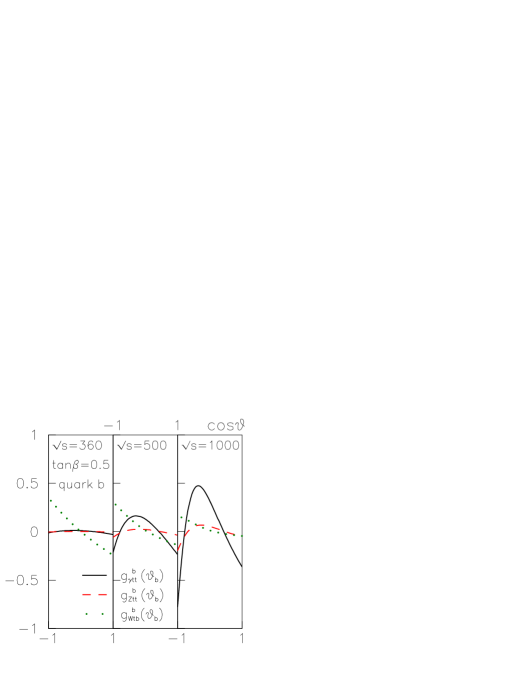
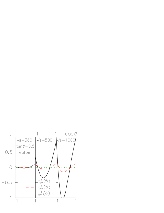
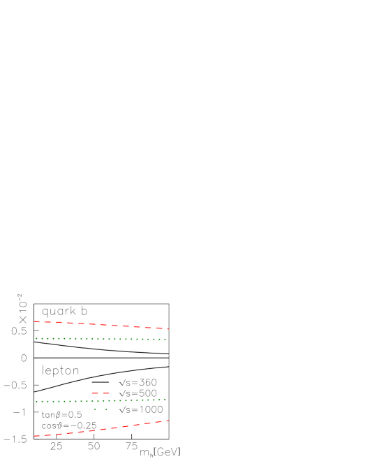
Adopting general formulas for the asymmetry from Ref. [45] and inserting form factors calculated here we plot the asymmetry in Figs.10, 11 as a function of $\cos\theta$ for bottom quarks and leptons, respectively. As before, the asymmetry can be decomposed into $\gamma t\bar{t}$, $Zt\bar{t}$ and $Wtb$ vertex contributions:

$${\cal A}_{CP}^{f}(\theta_{\!\scriptscriptstyle{f}})=g_{\gamma t\bar{t}}^{f}(\theta_{\!\scriptscriptstyle{f}})\ \Re D_{\gamma}+g_{Zt\bar{t}}^{f}(\theta_{\!\scriptscriptstyle{f}})\ \Re D_{Z}+g_{Wtb}^{f}(\theta_{\!\scriptscriptstyle{f}})\ \Re(f_{2}^{R}-\bar{f}_{2}^{L}).$$ (30)

It is seen that forward-backward directions are favored, however an experimental cut $|\cos\theta_{f}|<0.9$ should be imposed in the realistic experimental environment.

Figure 10: The coefficients functions $g$ defined by eq.(30) for the angular asymmetry, for final bottom quarks ($f=b$) as a function of $\cos\theta$ for $\sqrt{s}=$ 360 (left), 500 (middle) and 1000 GeV (right) for $\tan\beta=0.5$. The solid curve represents the coefficient $g_{\gamma t\bar{t}}^{f}(\theta_{\!\scriptscriptstyle{f}})$, dashed $g_{Zt\bar{t}}^{f}(\theta_{\!\scriptscriptstyle{f}})$ and dotted $g_{Wtb}^{f}(\theta_{\!\scriptscriptstyle{f}})$

Figure 11: The same as Fig.10 calculated for final leptons ($f=l$).

In order to illustrate the Higgs mass dependence we plot in Fig.12 the angular asymmetry both for $f=b$ and $f=l$ for chosen polar angle $\cos\theta=-0.25$. As expected the maximal effect could be reached for minimal Higgs mass $m_{h}=10\,{\rm GeV}$, $\sqrt{s}=500\,{\rm GeV}$ is the most suitable energy.

Figure 12: The Higgs mass dependence of the coefficient of $R_{i2}R_{i3}$ for the angular asymmetry defined by eq.(29) for $\sqrt{s}$=360 (solid), 500 (dashed), 1000 (dotted) GeV for a fixed polar angle $\cos\theta=-0.25$ and $\tan\beta=0.5$.

5.4 Integrated Angular Asymmetry

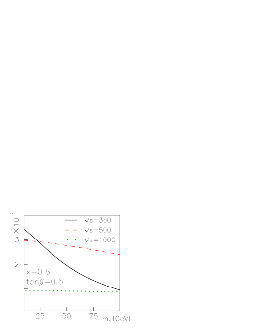
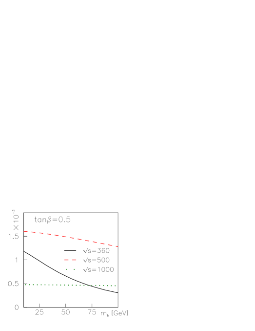
The angular distribution given in eq.(28) could be adopted to define an integrated version [41] of the angular asymmetry ${\cal A}_{CP}^{f}(\theta_{\!\scriptscriptstyle{f}})$:

$${\cal A}_{\scriptscriptstyle{CP}}^{\scriptscriptstyle{f}}(P_{e^{-}},P_{e^{+}})=\frac{{\displaystyle\int_{-c_{m}}^{0}\!d\cos\theta_{\!\scriptscriptstyle{f}}\frac{d\sigma^{+(*)}(\theta_{\!\scriptscriptstyle{f}})}{d\cos\theta_{\!\scriptscriptstyle{f}}}-\int_{0}^{+c_{m}}\!d\cos\theta_{\!\scriptscriptstyle{f}}\frac{d\sigma^{-(*)}(\theta_{\!\scriptscriptstyle{f}})}{d\cos\theta_{\!\scriptscriptstyle{f}}}}}{{\displaystyle\int_{-c_{m}}^{0}\!d\cos\theta_{\!\scriptscriptstyle{f}}\frac{d\sigma^{+(*)}(\theta_{\!\scriptscriptstyle{f}})}{d\cos\theta_{\!\scriptscriptstyle{f}}}+\int_{0}^{+c_{m}}\!d\cos\theta_{\!\scriptscriptstyle{f}}\frac{d\sigma^{-(*)}(\theta_{\!\scriptscriptstyle{f}})}{d\cos\theta_{\!\scriptscriptstyle{f}}}}},$$ (31)

where $P_{e^{-}}$ and $P_{e^{+}}$ are the polarizations of $e$ and $\bar{e}$ beams, $d\sigma^{+/-(*)}$ is referring to $f$ and $\bar{f}$ distributions respectively, and $c_{m}$ expresses the experimental polar-angle cut. In order to discuss possible advantages of polarized initial beams we are considering here dependence of the asymmetry on the polarization. Hereafter we will discuss the same polarization for $e$ and $\bar{e}$: $P\equiv P_{e^{-}}=P_{e^{+}}$.

Again we decompose the asymmetry as follows:

$${\cal A}_{CP}^{f}(P)=g_{\gamma t\bar{t}}^{f}(P)\ \Re D_{\gamma}+g_{Zt\bar{t}}^{f}(P)\ \Re D_{Z}+g_{Wtb}^{f}(P)\ \Re(f_{2}^{R}-\bar{f}_{2}^{L}).$$ (32)

In Table 2 we show the coefficient functions $g$ calculated for various energy and polarization choices assuming the polar angle cut $|\cos\theta_{\!\scriptscriptstyle{f}}|<0.9$, i.e. $c_{m}=0.9$ in eq.(31), both for leptons and bottom quarks . It could be seen that a positive polarization leads to higher coefficients $g_{\gamma t\bar{t}}^{f}$ and $g_{Zt\bar{t}}^{f}$. Since $\Re(D_{\gamma})>\Re(D_{Z})\gg\Re(f^{R}_{2}-\bar{f}^{L}_{2})$ that implies that maximal asymmetry could be reached for $P=+0.8$ and the dominant contribution is originating from $\Re(D_{\gamma})$. Since the number of events does not drop drastically when going from unpolarized beams to $P=+0.8$, it turns out that the positive polarization is the most suitable for testing the integrated angular asymmetry. It is clear from the table that the asymmetry for final leptons should be larger by a factor $3\div 4$ then the one for bottom quarks and their signs should be reversed.

$\sqrt{s}[\,{\rm GeV}]$	$P$	quark b						lepton
		$g_{\gamma t\bar{t}}^{b}(P)$		$g_{Zt\bar{t}}^{b}(P)$		$g_{Wtb}^{b}(P)$		$g_{\gamma t\bar{t}}^{l}(P)$		$g_{Zt\bar{t}}^{l}(P)$
360	0.0	0.	00844	0.	00106	0.	142	-0.	0162	-0.	00203
	0.8	0.	00983	-0.	00555	-0.	259	-0.	0493	0.	0278
	-0.8	0.	00758	0.	00510	0.	388	-0.	0106	-0.	00713
500	0.0	0.	113	0.	0136	0.	121	-0.	224	-0.	0270
	0.8	0.	131	-0.	0718	-0.	247	-0.	627	0.	343
	-0.8	0.	101	0.	0661	0.	347	-0.	149	-0.	0968
1000	0.0	0.	332	0.	0389	0.	0678	-0.	722	-0.	0845
	0.8	0.	422	-0.	225	-0.	167	-1.	55	0.	824
	-0.8	0.	284	0.	181	0.	194	-0.	507	-0.	322

Table 2: The energy and polarization dependence of the coefficients $g_{\gamma t\bar{t}}^{f}(P)$, $g_{Zt\bar{t}}^{f}(P)$ and $g_{Wtb}^{f}(P)$ defined in eq.(32) for leptons ($f=l$) and bottom quarks ($f=b$).

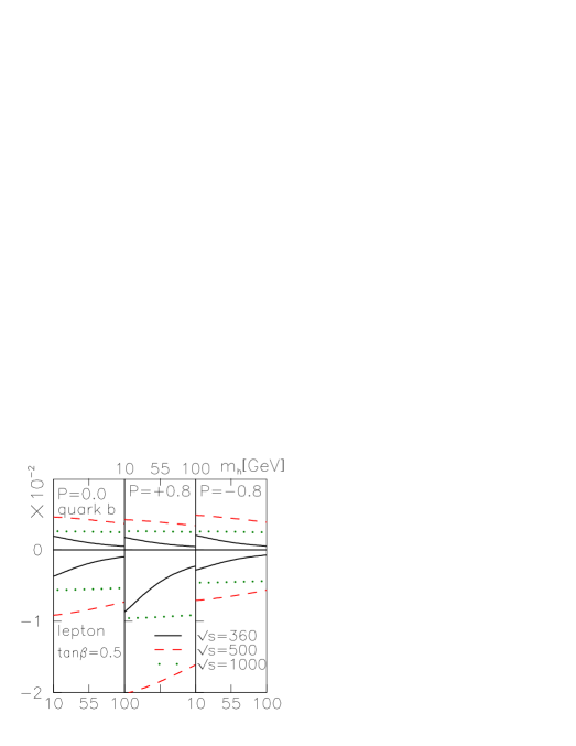
Using the general formula for the asymmetry from Ref. [41] and adopting results for the CP-violating form factors we plot ${\cal A}_{\scriptscriptstyle{CP}}^{\scriptscriptstyle{f}}(P_{e^{-}},P_{e^{+}})$ in Fig.13 as a function of the Higgs mass both for bottom quarks and leptons. It is clear that the largest asymmetry could be expected for $P_{e^{-}}=P_{e^{+}}=+0.8$ for final leptons at $\sqrt{s}=500\,{\rm GeV}$. With the maximal mixing, $R_{i2}R_{i3}=1/2$ the $1\%$ asymmetry could be expected for the Higgs boson with mass $m_{h}=10\div 20\,{\rm GeV}$. Since the statistical error expected [41] for the asymmetry is of the order of $5\times 10^{-3}$, we can conclude that the asymmetry ${\cal A}_{\scriptscriptstyle{CP}}^{\scriptscriptstyle{f}}(P_{e^{-}},P_{e^{+}})$ is the most promising one, leading to $2\sigma$ effect for light Higgs mass and $\tan\beta=0.5$. As it is seen form Fig.13 it is relevant to have polarized $e^{+}e^{-}$ beams.

Figure 13: The Higgs mass dependence of the coefficient of $R_{i2}R_{i3}$ for the angular asymmetry defined by eq.(31) for bottom quarks (upper) and leptons (lower) at $\sqrt{s}$=360 (solid), 500 (dashed), 1000 GeV (dotted) with unpolarized beams (left), $P=+0.8$ (middle) and $P=-0.8$ (right) for $\tan\beta=0.5$.

6 Summary and Conclusions

We have considered a general two-Higgs-doublet model with CP violation in the scalar sector. Mixing of the three neutral Higgs fields of the model leads to CP-violating Yukawa couplings of the physical Higgs bosons. CP-asymmetric form factors generated at the one-loop level of perturbation theory has been calculated within the model. Although in general the existing experimental data from LEP1 and LEP2 constraint the mixing angles of the three neutral Higgs fields, their combination relevant for CP violation is not bounded for small $\tan\beta$ which is the region of our interest. We have shown that the decay form factors are typically smaller then the production ones by 2-3 orders of magnitude. The dominant contribution to CP violation in the production is coming from $\gamma t\bar{t}$ coupling. Several energy and angular CP-violating asymmetries for the process $e^{+}e^{-}\to t\bar{t}\to l^{\pm}\cdots$ and $e^{+}e^{-}\to t\bar{t}\to\stackrel{{\scriptstyle{\scriptscriptstyle(-)}}}{{b}}\cdots$ has been considered using the form factors calculated within the two-Higgs-doublet model. It turned out that the best test of CP invariance would be provided by the integrated angular asymmetry ${\cal A}_{\scriptscriptstyle{CP}}^{\scriptscriptstyle{f}}(P_{e^{-}},P_{e^{+}})$ for positive polarizations of $e^{+}e^{-}$ beams. For one year of running at TESLA collider with the integrated luminosity $L=500\;{\hbox{fb}^{-1}}{\hbox{y}^{-1}}$ one could expect $2\sigma$ effect for the asymmetry for light Higgs boson and $\tan\beta=0.5$.

Acknowledgments

This work was supported in part by the Committee for Scientific Research (Poland) under grants No. 2 P03B 014 14 and No. 2 P03B 080 19.

A Appendix

A.1 1-Loop Integrals

Figure 14: Convention for momenta and mass labelling used.

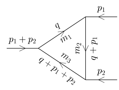
Here we will define 3-point one-loop integrals used in calculations of form factors. The convention for momenta and mass labelling is presented in Fig.14. The Passarino-Veltman functions [21] ${\mathbf{C}}$ are defined as follows:

$$\mu^{4-n} \int\frac{d^{n}k}{(2\pi)^{n}}\frac{1;k_{\mu};k_{\mu}k_{\nu}}{[k^{2}-m_{1}^{2}][(k+p_{1})^{2}-m_{2}^{2}][(k+p_{1}+p_{2})^{2}-m_{3}^{2}]}$$ (33)

$$=\frac{i}{16\pi^{2}}{\mathbf{C}}_{0;\mu;\mu\nu}(p_{1}^{2},p_{2}^{2},p^{2};m_{1}^{2},m_{2}^{2},m_{3}^{2}).$$

The vector and tensor integrals ${\mathbf{C}}_{\mu}$ and ${\mathbf{C}}_{\mu\nu}$ can be expanded into scalar coefficients and Lorentz covariants:

$${\mathbf{C}}^{\mu} = p_{1}^{\mu}{\mathbf{C}}_{11}+p_{2}^{\mu}{\mathbf{C}}_{12}$$ (34)

$${\mathbf{C}}^{\mu\nu} = p_{1}^{\mu}p_{1}^{\nu}{\mathbf{C}}_{21}+p_{2}^{\mu}p_{2}^{\nu}{\mathbf{C}}_{22}+(p_{1}^{\mu}p_{2}^{\nu}+p_{2}^{\mu}p_{1}^{\nu}){\mathbf{C}}_{23}+g^{\mu\nu}{\mathbf{C}}_{24}.$$ (35)

Imaginary part of ${\mathbf{C}}_{12}$ for certain sets of arguments is needed for the calculation of $\Re D_{\gamma}$ and $\Re D_{Z}$:

$$\Im{\mathbf{C}}_{12}(p_{t},p_{\bar{t}};m_{t},m_{h},m_{t})=\frac{\pi}{s\beta_{t}}\left[1-\frac{h^{2}}{\beta_{t}^{2}}\log\left(1+\frac{\beta_{t}^{2}}{h^{2}}\right)\right]\Theta(\sqrt{s}-2m_{t})$$

$$\Im{\mathbf{C}}_{12}(p_{t},p_{\bar{t}};m_{h},m_{t},m_{Z})=\frac{\pi}{s\beta_{t}^{2}}\times$$ (36)

$$\left\{\left[2t^{2}(1-h^{2}-z^{2})-h^{2}\beta_{t}^{2}\right]\frac{1}{\beta_{t}}\log\left(\frac{1-z^{2}-h^{2}-\beta_{t}\beta_{Z}}{1-z^{2}-h^{2}+\beta_{t}\beta_{Z}}\right)+\beta_{Z}\right\}\Theta(\sqrt{s}-m_{h}-m_{Z}),$$

for $h\equiv m_{h}/\sqrt{s}$, $\beta_{t}=\sqrt{1-4m_{t}^{2}/s}$ and $\beta_{Z}=\lambda(1,z^{2},h^{2})$, where $\lambda(a,b,c)$ is the standard kinematic function.

In order to calculate $\hbox{Re}(f^{R}_{2}-\bar{f}^{L}_{2})$ one needs an imaginary part of the following ${\mathbf{C}}_{22}$ function. Neglecting $m_{b}$ and defining $\hat{m}_{W}\equiv\frac{m_{W}}{\omega m_{t}}$ and $\hat{m}_{h}\equiv\frac{m_{h}}{\omega m_{t}}$ for $\omega=1-m_{W}^{2}/m_{t}^{2}$ one gets:

$$\Im{\mathbf{C}}_{22}(p_{W},p_{b},m_{W}^{2},m_{h}^{2},m_{b}^{2})=\frac{\pi\omega}{2m_{t}^{2}}\left\{\left[2\hat{m}_{h}^{2}(6\hat{m}_{W}^{2}+1)-(2\hat{m}_{W}^{2}+1)\right]+\right.$$

$$\left.-2\left[\hat{m}_{h}^{2}(6\hat{m}_{W}^{2}+1)+2\hat{m}_{W}^{2}\right]\hat{m}_{h}^{2}\log\left(1+\hat{m}_{h}^{-2}\right)\right\}.$$ (37)

A.2 Asymptotic Formulae

A.2.1 Production of $t\bar{t}$

For $h\equiv\frac{m_{h}}{\sqrt{s}}$ in the limit $\frac{h^{2}}{\beta_{t}^{2}}\ll 1$ one gets:

$$\Re D_{\gamma}=-\frac{t^{2}}{2\pi\beta_{t}}\frac{m_{t}^{2}}{v^{2}}A_{\gamma}b_{t}a_{t}\left[1+\frac{h^{2}}{\beta_{t}^{2}}\log\left(\frac{h^{2}}{\beta_{t}^{2}}\right)\right]\Theta(1-4t^{2})$$ (38)

$$\Re D_{Z}=-\frac{1}{2\pi\beta_{t}^{3}}\frac{m_{t}^{2}}{v^{2}}A_{Z}b_{t}\left\{a_{t}t^{2}\beta_{t}^{2}\left[1+\frac{h^{2}}{\beta_{t}^{2}}\log\left(\frac{h^{2}}{\beta_{t}^{2}}\right)\right]\Theta(1-4t^{2})+\right.\\ -C_{i}z^{2}\left[\beta_{t}(1-h^{2}-z^{2})+(2t^{2}(1-h^{2}-z^{2})-h^{2}\beta_{t}^{2})\log\left(\frac{1-\beta_{t}}{1+\beta_{t}}\right)\right]\\ \left.\Theta{}(1-h-z),\right\}$$ (39)

where $z\equiv m_{Z}/\sqrt{s}$ and $t\equiv m_{t}/\sqrt{s}$.

For $\frac{h^{2}}{\beta_{t}^{2}s}\gg 1$ one gets:

$$\Re D_{\gamma} = -\frac{t^{2}}{12\pi\beta_{t}}\frac{m_{t}^{2}}{v^{2}}A_{\gamma}b_{t}a_{t}\frac{\beta_{t}^{2}}{h^{2}}(3-2\frac{\beta_{t}^{2}}{h^{2}})\Theta(1-4t^{2})$$

$$\Re D_{Z} = -\frac{t^{2}}{12\pi\beta_{t}}\frac{m_{t}^{2}}{v^{2}}A_{Z}b_{t}a_{t}\frac{\beta_{t}^{2}}{h^{2}}(3-2\frac{\beta_{t}^{2}}{h^{2}})\Theta(1-4t^{2})$$ (40)

A.2.2 Decay of the Top Quark

In the limit $\hat{m}_{h}\equiv\frac{m_{h}}{\omega m_{t}}\ll 1$:

$$\Re(f_{2}^{R}|_{CPV})=\frac{g^{2}b_{b}C_{i}}{64\pi}\left(\frac{m_{b}}{m_{t}}\right)^{2}\hat{m}_{W}\left\{-(1+\frac{1}{2}\hat{m}_{W}^{-2})+\left[6+\hat{m}_{W}^{-2}+2\log(\hat{m}^{2}_{h})\right]\hat{m}^{2}_{h}\right\},$$ (41)

while for $\hat{m}_{h}\gg 1$:

$$\Re(f_{2}^{R}|_{CPV})=\frac{g^{2}b_{b}C_{i}}{64\pi}\left(\frac{m_{b}}{m_{t}}\right)^{2}\hat{m}_{W}^{-1}\hat{m}_{h}^{-2}\left[-(\hat{m}_{W}^{2}+\frac{1}{3})+(\frac{5}{6}\hat{m}_{W}^{2}+\frac{1}{4})\hat{m}^{-2}_{h}\right].$$ (42)

10

References

- [1] Abe, F. et al., Phys. Rev. Lett. 73 (1994) 225, hep-ex/9405005
- [2] Abachi, S. et al., Phys. Rev. Lett. 74 (1995) 2632, hep-ex/9503003
- [3] Kobayashi, M. and Maskawa, T., Prog. Theor. Phys. 49 (1973) 652
- [4] Gavela, M. B., Hernandez, P., Orloff, J., Pene, O., and Quimbay, C., Nucl. Phys. B430 (1994) 382, hep-ph/9406289
- [5] Huet, P. and Sather, E., Phys. Rev. D51 (1995) 379, hep-ph/9404302
- [6] Lee, T. D., Phys. Rev. D8 (1973) 1226
- [7] Weinberg, S., Phys. Rev. D42 (1990) 860, KEK-199005425
- [8] Branco, G. C. and Rebelo, M. N., Phys. Lett. B160 (1985) 117
- [9] Gunion, J. F., Haber, H. E., Kane, G. L., and Dawson, S., The Higgs Hunter’s Guide, Addison-Wesley Publishing Company, 1989
- [10] Han, T. and Jiang, J., (2000), hep-ph/0011271
- [11] Groom, D. E. et al., Eur. Phys. J. C15 (2000) 1
- [12] Bigi, I. I. Y. and Krasemann, H., Zeit. Phys. C7 (1981) 127
- [13] Kuhn, J. H.
- [14] Bigi, I. I. Y., Dokshitzer, Y. L., Khoze, V., Kuhn, J., and Zerwas, P., Phys. Lett. B181 (1986) 157
- [15] Czarnecki, A. and Krause, B., Phys. Rev. Lett. 78 (1997) 4339, hep-ph/9704355
- [16] Grzadkowski, B. and Keung, W.-Y., Phys. Lett. B319 (1993) 526, hep-ph/9310286
- [17] Chang, D., Keung, W.-Y., and Phillips, I., Nucl. Phys. B408 (1993) 286, hep-ph/9301259
- [18] Bernreuther, W., Schroder, T., and Pham, T. N., Phys. Lett. B279 (1992) 389
- [19] Grzadkowski, B. and Gunion, J. F., Phys. Lett. B287 (1992) 237
- [20] Atwood, D., Bar-Shalom, S., Eilam, G., and Soni, A., (2000), hep-ph/0006032
- [21] Passarino, G. and Veltman, M., Nucl. Phys. B160 (1979) 151
- [22] Guth, R. J. and Kuhn, J. H., Nucl. Phys. B368 (1992) 38
- [23] Branco, G. C., Lavoura, L., and Silva, J. P., CP violation, Oxford University Press, 1999
- [24] Hasuike, T., Hattori, T., and Wakaizumi, S., Phys. Rev. D58 (1998) 095008, hep-ph/9911526
- [25] Hasuike, T., Hattori, T., Hayashi, T., and Wakaizumi, S., Z. Phys. C76 (1997) 127, hep-ph/9611304
- [26] Affolder, T. et al., Phys. Rev. Lett. 84 (2000) 216, hep-ex/9909042
- [27] Cho, P. and Misiak, M., Phys. Rev. D49 (1994) 5894, hep-ph/9310332
- [28] Fujikawa, K. and Yamada, A., Phys. Rev. D49 (1994) 5890
- [29] Bernreuther, W., Nachtmann, O., Overmann, P., and Schroder, T., Nucl. Phys. B388 (1992) 53
- [30] Greub, C., (1999), hep-ph/9911348
- [31] Grzadkowski, B. and Pliszka, J., work in progress
- [32] Gunion, J. F., Grzadkowski, B., Haber, H. E., and Kalinowski, J., Phys. Rev. Lett. 79 (1997) 982, hep-ph/9704410
- [33] Abreu, P. et al., Eur. Phys. J. C12 (2000) 567
- [34] Abbiendi, G. et al., (2000), hep-ex/0007040
- [35] Chankowski, P. H., Krawczyk, M., and Zochowski, J., Eur. Phys. J. C11 (1999) 661, hep-ph/9905436
- [36] Gunion, J. F. and Grzadkowski, B., Phys. Lett. B243 (1990) 301
- [37] Haber, H. E. and Logan, H. E., Phys. Rev. D62 (2000) 015011, hep-ph/9909335
- [38] Abbiendi, G. et al., Eur. Phys. J. C7 (1999) 407, hep-ex/9811025
- [39] ALEPH, Searches for higgs bosons: preliminary combined results using lep data collected at energies up to 202 gev, ALEPH 2000-028 CONF 2000-023
- [40] Ackerstaff, K. et al., Eur. Phys. J. C5 (1998) 19, hep-ex/9803019
- [41] Grzadkowski, B. and Hioki, Z., Nucl. Phys. B585 (2000) 3, hep-ph/0004223
- [42] Grzadkowski, B. and Hioki, Z., Nucl. Phys. B484 (1997) 17, hep-ph/9604301
- [43] Brzezinski, L., Grzadkowski, B., and Hioki, Z., Int. J. Mod. Phys. A14 (1999) 1261, hep-ph/9710358
- [44] Grzadkowski, B. and Hioki, Z., Phys. Lett. B391 (1997) 172, hep-ph/9608306
- [45] Grzadkowski, B. and Hioki, Z., Phys. Lett. B476 (2000) 87, hep-ph/9911505
- [46] Rindani, S. D., Pramana 54 (2000) 791, hep-ph/0002006