Angular distributions in hard exclusive production of pion pairs

Abstract

Using the leading order amplitudes of hard exclusive electroproduction of pion pairs we have analyzed the angular distribution of the two produced particles. At leading twist a pion pair can be produced only in an isovector or an isoscalar state. We show that certain components of the angular distribution only get contributions from the interference of the $I=1$ and the (much smaller) $I=0$ amplitude. Therefore our predictions prove to be a good probe of isospin zero pion pair production. We predict effects of a measurable size that could be observed at experiments like HERMES. We also discuss how hard exclusive pion pair production can provide us with new information on the effective chiral Lagrangian.

I Introduction

The factorization theorem [1] states that the amplitude of the exclusive production process

$$\gamma^{\ast}_{L}+T\to F+T^{\prime}$$ (1)

at large invariant collision energy $\sqrt{s}\to\infty$, large virtuality of the (longitudinally polarized) photon $Q^{2}\to\infty$, fixed $Q^{2}/s$ (Bjorken limit), and with $-t,m_{T}^{2},m_{T^{\prime}}^{2},m_{F}^{2}\ll Q^{2}$ can be written in the form

$$\sum_{i,j}\int{\mathrm{d}}z{\mathrm{d}}x_{1}f_{i/T}^{T^{\prime}}(x_{1},x_{1}-x_{{\mathrm{B}j}},t)\,H_{ij}\Big{(}\frac{x_{1}}{x_{{\mathrm{B}j}}},Q^{2},z\Big{)}\,\Phi^{F}_{j}(z)+\mbox{power-suppressed corrections}\,,$$ (2)

where $H_{ij}$ is a hard part computable in pQCD as a series in $\alpha_{{\mathrm{s}}}$, $\Phi^{F}_{j}$ is the distribution amplitude of the hadronic state $F$, and $f_{i/T}^{T^{\prime}}$ is a $T\to T^{\prime}$ skewed parton distribution [1, 2, 3, 4] (for a review see [5]). Skewed parton distributions (SPD’s) are related to matrix elements of bilocal operators between states of different momentum. They are generalizations of the usual parton distributions which parameterize the diagonal matrix elements of the corresponding operators. Therefore hard exclusive electroproduction opens a new way to study the partonic structure of hadrons. Naturally, for the experimentally accessible range of $Q^{2}$ the size of the $1/Q$ suppressed power corrections can be rather large, the quantitative estimates of higher twist corrections are therefore in the focus of recent investigation [6]. Still, the formalism has been used to investigate exclusive production of single light mesons [1, 7, 8, 9, 10]. For the starting point of the present work it is important to note that the factorization theorem is not limited to the case where the produced hadronic state $F$ in reaction (1) is a one particle state provided that its invariant mass is small compared to $Q$ [11].

In the present paper we present a detailed analysis of hard exclusive electroproduction of two pions to leading order in the strong coupling constant $\alpha_{{\mathrm{s}}}$. In that case $\Phi^{F}_{j}$ in the expression (2) is a two-pion distribution amplitude ($2\pi$DA). At leading twist the pion pair can be produced in a state with isospin one or zero. For $I=1$ the process is dominated by the $\rho$ peak. (So in a certain sense our approach can be considered as an alternative description of $\rho$ production, which has been studied earlier using a distribution amplitude for the $\rho$ meson [1, 7, 8, 9, 10]). The description of pion pair production at small $x_{{\mathrm{B}j}}$ in terms of $2\pi$DA’s was considered in Ref. [12], where it was demonstrated that such a description allows us to determine the details of the partonic structure of the pion and the $\rho$ meson from data on the di-pion mass distributions in hard diffraction alone.

Here we are mainly interested in the production of $I=0$ pion pairs. It seems to be difficult to investigate isoscalar pair production by the measurement of total cross sections because identifying $\pi^{0}\pi^{0}$ production events would require detecting 4 correlated photons whereas $\pi^{+}\pi^{-}$ production is dominated by the isovector contribution due to the $\rho$ resonance (see our analysis in [13]). However, the angular distribution of the produced pion pairs contains components that depend only on the interference of the $I=0$ and the $I=1$ channel [13, 14]. Using specific models for the involved SPD’s and $2\pi$DA’s we predict effects of a measurable size and suggest the most favorable kinematic range for such measurements.

The interesting feature of hard exclusive production of pion pairs in an isoscalar state is that the pions are produced not only by a collinear $q\bar{q}$ pair but also (and in the same order in $1/Q$ and $\alpha_{{\mathrm{s}}}$) by two collinear gluons. This observation opens a possibility to access the gluon content of the isoscalar $\pi\pi$ states. In the analysis of the present work we shall assume that the elusive isoscalar $\pi\pi$ resonance $f_{0}(400-1200)$ has no anomalously large gluon contents as it was suggested e.g. in [15, 16]. The use of hard exclusive pion pair production for “gluonometry” of the low-lying isoscalar resonances will be considered elsewhere.

II Amplitudes and intensity densities

In this section we calculate the amplitude of hard two-pion electroproduction to leading order in $1/Q^{2}$ and $\alpha_{{\mathrm{s}}}$ in terms of SPD’s and $2\pi$DA’s and show how they are connected to the so called intensity densities which we define as

$$\langle P_{l}(\cos\theta)\rangle^{\pi\pi}:=\frac{\int_{-1}^{1}{\mathrm{d}}\cos\theta\,P_{l}(\cos\theta)\,\frac{{\mathrm{d}}\sigma^{\pi\pi}}{{\mathrm{d}}\cos\theta}}{\int_{-1}^{1}{\mathrm{d}}\cos\theta\,\frac{{\mathrm{d}}\sigma^{\pi\pi}}{{\mathrm{d}}\cos\theta}}\,.$$ (3)

FIG. 1.: Definition of the scattering angle $\theta$.

Here $\theta$ is defined as the scattering angle of the $\pi^{+}$ or one $\pi^{0}$ (for $\pi^{+}\pi^{-}$ or $\pi^{0}\pi^{0}$ production respectively) in the center of mass system of the two pions with respect to their total momentum e.g. in the laboratory system (see Fig. 1).

We consider the process

$$\gamma_{L}^{*}(q)+B_{1}(p)\to\pi\pi(q^{\prime})+B_{2}(p+\Delta)\,,$$ (4)

where a linear polarized virtual photon with momentum $q$ and a nucleon $B_{1}$ with momentum $p$ produce a final state with a baryon $B_{2}$ (a nucleon or a heavier state) with momentum $p^{\prime}=p+\Delta$ and a pion pair with total momentum $q^{\prime}$. Note that the amplitude for the corresponding production process with a transversally polarized virtual photon is $1/Q$ power suppressed (with $Q^{2}=-q^{2}$). Therefore the (sub-) process (4) with a longitudinally polarized photon is the only leading contribution to the electroproduction reaction $e^{-}(l)+B_{1}(p)\to\pi\pi(q^{\prime})+e^{-}(l-q)+B_{2}(p+\Delta)$. Using two light cone vectors $n$ and $\tilde{n}$ normalized such that

$$n\cdot(p+p^{\prime})=2\,,\hskip 28.45274pt\tilde{n}\cdot n=1$$ (5)

the relevant momenta can be expressed as

$$p^{\mu} = (1+\xi)\tilde{n}^{\mu}+(1-\xi)\frac{\bar{m}^{2}}{2}n^{\mu}-\frac{1}{2}\Delta_{\perp}^{\mu}$$ (6)

$$p^{\prime\mu} = (1-\xi)\tilde{n}^{\mu}+(1+\xi)\frac{\bar{m}^{2}}{2}n^{\mu}+\frac{1}{2}\Delta_{\perp}^{\mu}$$ (7)

$$q^{\mu} = -2\tilde{\xi}\tilde{n}^{\mu}+\frac{Q^{2}}{4\tilde{\xi}}n^{\mu}$$ (8)

with

$$\bar{m}^{2} = \frac{1}{2}\Bigl{(}m_{B_{1}}^{2}+m_{B_{2}}^{2}-\frac{t}{2}\Bigr{)}$$ (9)

$$\tilde{\xi} = \xi\Bigl{(}1-\frac{1}{Q^{2}}(q^{\prime 2}-t-4\xi^{2}\bar{m}^{2})\Bigr{)}+{\cal O}\Big{(}\frac{1}{Q^{4}}\Big{)}\,.$$ (10)

$\Delta_{\perp}$ is defined to be that spacelike component of the momentum transfer $\Delta$ which is transverse to the light cone vectors $n$ and $\tilde{n}$, $t$ is the momentum transfer squared $t=\Delta^{2}$, and $\xi$ is the skewedness parameter describing the longitudinal component of the momentum transfer

$$\xi=-\frac{1}{2}(n\cdot\Delta)\,,$$ (11)

which in the Bjorken limit $Q^{2}\to\infty$ can be expressed in terms of the Bjorken variable $x_{{\mathrm{B}j}}=\frac{Q^{2}}{2p\cdot q}$ as

$$\xi=\frac{x_{{\mathrm{B}j}}}{2-x_{{\mathrm{B}j}}}\,.$$ (12)

FIG. 2.: Examples of the three classes of leading order diagrams for hard exclusive pion pair production.

The leading order amplitude for the reaction (4) corresponds to diagrams of the type shown in Fig. 2 and has the form (see also [13, 14])

$$T^{\pi^{a}\pi^{b}} = \langle B_{2}(p^{\prime}),\pi^{a}\pi^{b}(q^{\prime})|J^{\mathrm{e}.m.}\cdot\varepsilon_{L}|B_{1}(p)\rangle$$ (13)

$$= -(e4\pi\alpha_{s})\frac{1}{2Q}\int_{-1}^{1}{\mathrm{d}}\tau\int_{0}^{1}{\mathrm{d}}z$$ (17)

$$\times\Biggl{\{}\frac{C_{F}}{N_{c}}\sum_{f,f^{\prime}}F_{ff^{\prime}}(\tau,\xi,t)\Phi_{f^{\prime}f}^{ab}(z,\zeta,m_{\pi\pi})\biggl{[}\frac{e_{f^{\prime}}}{z(\tau+\xi-{\mathrm{i}}\epsilon)}+\frac{e_{f}}{(1-z)(\tau-\xi+{\mathrm{i}}\epsilon)}\biggr{]}$$

$$\;\;-\frac{1}{N_{c}}\sum_{f}e_{f}F_{ff}(\tau,\xi,t)\Phi_{G}^{ab}(z,\zeta,m_{\pi\pi})\frac{1}{z(1-z)}\biggl{[}\frac{1}{\tau+\xi-{\mathrm{i}}\epsilon}-\frac{1}{\tau-\xi+{\mathrm{i}}\epsilon}\biggr{]}$$

$$\;\;+\frac{1}{2N_{c}}\sum_{f}e_{f}F_{G}(\tau,\xi,t)\Phi_{ff}^{ab}(z,\zeta,m_{\pi\pi})\frac{1}{z(1-z)}\biggl{[}\frac{1}{\tau+\xi-{\mathrm{i}}\epsilon}+\frac{1}{\tau-\xi+{\mathrm{i}}\epsilon}\biggr{]}\Biggr{\}}\,,$$

where $e_{f}$ is the electric charge of a quark of flavor $f$ in units of the proton charge $e$ and $\varepsilon_{L}^{\mu}$ is the longitudinal photon polarization vector

$$\varepsilon_{L}^{\mu}=\frac{2\tilde{\xi}}{Q}\tilde{n}^{\mu}+\frac{Q}{4\tilde{\xi}}n^{\mu}$$ (18)

($\Rightarrow\varepsilon_{L}^{\mu}=\frac{1}{Q}(q^{3},0,0,q^{0})$ in a frame with $n^{\mu}\propto(1,0,0,1)$ and $\tilde{n}^{\mu}\propto(1,0,0,-1)$). The functions $F_{ff^{\prime}}(\tau,\xi,t)$ and $F_{G}(\tau,\xi,t)$ are skewed parton distributions for quarks or gluons respectively defined as

$$F_{ff^{\prime}}(\tau,\xi,t) = \int\frac{{\mathrm{d}}\lambda}{2\pi}e^{{\mathrm{i}}\lambda\tau}\langle B_{2}(p^{\prime})|T\Big{[}\bar{\psi}_{f^{\prime}}\!\Big{(}\!-\!\frac{\lambda n}{2}\Big{)}{/n}\psi_{f}\!\Big{(}\frac{\lambda n}{2}\Big{)}\Big{]}|B_{1}(p)\rangle$$ (19)

$$F_{G}(\tau,\xi,t) = \frac{1}{\tau}\int\frac{{\mathrm{d}}\lambda}{2\pi}e^{{\mathrm{i}}\lambda\tau}n^{\mu}n^{\nu}\langle B_{2}(p^{\prime})|T\Big{[}F_{\mu}^{A\alpha}\!\Big{(}\!-\!\frac{\lambda n}{2}\Big{)}F^{A}_{\alpha\nu}\!\Big{(}\frac{\lambda n}{2}\Big{)}\Big{]}|B_{1}(p)\rangle\,.$$ (20)

The gluon color index $A$ is understood to be summed over. The two-pion distribution amplitudes

$$\Phi_{f^{\prime}f}^{ab}(z,\zeta,m_{\pi\pi}) := \int\frac{{\mathrm{d}}\lambda}{2\pi}e^{-{\mathrm{i}}\lambda z(q^{\prime}\cdot\tilde{n})}\langle\pi^{a}\pi^{b}|T\big{[}\bar{\psi}_{f}(\lambda\tilde{n}){/\tilde{n}}\psi_{f^{\prime}}(0)\big{]}|0\rangle$$ (21)

and

$$\Phi^{ab}_{G}(z,\zeta,m_{\pi\pi}) := \frac{1}{\tilde{n}\cdot q^{\prime}}\int\frac{{\mathrm{d}}\lambda}{2\pi}e^{-{\mathrm{i}}\lambda z(q^{\prime}\cdot\tilde{n})}\tilde{n}^{\mu}\tilde{n}^{\nu}\langle\pi^{a}\pi^{b}|T\big{[}F_{\mu}^{A\alpha}(\lambda\tilde{n})F^{A}_{\alpha\nu}(0)\big{]}|0\rangle$$ (22)

describe how a pion pair is produced by two quarks or gluons respectively. The variable $z$ is the fraction of the longitudinal (along the vector $n$) meson pair momentum $q^{\prime}=q-\Delta$ carried by one of the two partons. The variable $\zeta$ characterizes the distribution of the longitudinal component of $q^{\prime}$ between the two pions and is given in terms of the momentum $k^{a}$ of the pion $\pi^{a}$ and the total momentum of the pion pair $q^{\prime}$ by

$$\zeta=\frac{k^{a}\cdot\tilde{n}}{q^{\prime}\cdot\tilde{n}}\,.$$ (23)

Let us note that $\zeta$ is related to the angle $\theta$ defined above by

$$\beta\cos\theta=2\zeta-1\quad{\mathrm{w}ith}\quad\beta:=\sqrt{1-\frac{4m_{\pi}^{2}}{m_{\pi\pi}^{2}}}\,.$$ (24)

In the definitions (19) – (22) a gauge link of the form ${\cal P}[\exp({\mathrm{i}}g\int_{z_{2}}^{z_{1}}A_{\mu}{\mathrm{d}}z^{\mu})]$ with $A_{\mu}=\sum_{A}t^{A}A^{A}_{\mu}$ is implied to be inserted between the two operators at different space–time coordinates. Also we do not write out explicitly the scale dependence of the SPD’s and $2\pi$DA’s.

In the following we will restrict ourselves to the case where $B_{1}$ and $B_{2}$ both are proton states. Then the pion pair can be either $\pi^{+}\pi^{-}$ or $\pi^{0}\pi^{0}$. The $2\pi$DA’s (21) and (22) can be isospin decomposed and expressed in terms of only two independent quark $2\pi$DA’s corresponding to isospin $I=0$ and $I=1$ pair production respectively and one single gluon $2\pi$DA. For $\pi^{+}\pi^{-}$ production we have

$$\Phi^{\pi^{+}\pi^{-}}_{f^{\prime}f}(z,\zeta,m_{\pi\pi}) = \delta^{f^{\prime}f}\Phi^{I=0}(z,\zeta,m_{\pi\pi})+\tau_{3}^{f^{\prime}f}\Phi^{I=1}(z,\zeta,m_{\pi\pi})$$ (25)

$$\Phi^{\pi^{+}\pi^{-}}_{G}(z,\zeta,m_{\pi\pi}) = \Phi^{G}(z,\zeta,m_{\pi\pi})$$ (26)

and for $\pi^{0}\pi^{0}$ production

$$\Phi^{\pi^{0}\pi^{0}}_{f^{\prime}f}(z,\zeta,m_{\pi\pi}) = \delta^{f^{\prime}f}\Phi^{I=0}(z,\zeta,m_{\pi\pi})$$ (27)

$$\Phi^{\pi^{0}\pi^{0}}_{G}(z,\zeta,m_{\pi\pi}) = \Phi^{G}(z,\zeta,m_{\pi\pi})\,.$$ (28)

Taking into account the $C$-invariance of the underlying theory one can easily derive the following symmetry properties for the three $2\pi$DA’s:

$$\Phi^{I=0}(z,\zeta,m_{\pi\pi}) = -\Phi^{I=0}(1-z,\zeta,m_{\pi\pi})=\Phi^{I=0}(z,1-\zeta,m_{\pi\pi})$$ (29)

$$\Phi^{I=1}(z,\zeta,m_{\pi\pi}) = \Phi^{I=1}(1-z,\zeta,m_{\pi\pi})=-\Phi^{I=1}(z,1-\zeta,m_{\pi\pi})$$ (30)

$$\Phi^{G}(z,\zeta,m_{\pi\pi}) = \Phi^{G}(1-z,\zeta,m_{\pi\pi})=\Phi^{G}(z,1-\zeta,m_{\pi\pi})$$ (31)

Using the decompositions (25) – (28) and the symmetry relations (29), (30) the transition amplitudes (17) for $\pi^{+}\pi^{-}$ and $\pi^{0}\pi^{0}$ production and an elastically scattered proton target can be written in the form

$$T^{\pi^{+}\pi^{-}} = T^{I=0}+T^{I=1}$$ (32)

$$T^{\pi^{0}\pi^{0}} = T^{I=0}$$ (33)

with

$$T^{I=0} = -(e4\pi\alpha_{{\mathrm{s}}})\frac{C_{F}}{N_{c}}\frac{1}{12Q}\,\tilde{\Phi}^{I=0}\Bigl{(}2I_{u}^{-}-I_{d}^{-}\Bigr{)}$$ (34)

$$T^{I=1} = -(e4\pi\alpha_{{\mathrm{s}}})\frac{C_{F}}{N_{c}}\frac{1}{12Q}\,\tilde{\Phi}^{I=1}\Bigl{(}2I_{u}^{+}+I_{d}^{+}+\frac{3}{C_{F}}I_{G}\Bigr{)}\,.$$ (35)

Here $\tilde{\Phi}^{I=0}$ and $\tilde{\Phi}^{I=1}$ are functions of $m_{\pi\pi}$ and $\cos\theta$ defined as

$$\tilde{\Phi}^{I=0} = \int_{0}^{1}{\mathrm{d}}z\frac{(1-2z)\Phi^{I=0}(z,\zeta,m_{\pi\pi})-\frac{2}{C_{F}}\Phi^{G}(z,\zeta,m_{\pi\pi})}{z(1-z)}$$ (36)

$$\tilde{\Phi}^{I=1} = \int_{0}^{1}{\mathrm{d}}z\frac{\Phi^{I=1}(z,\zeta,m_{\pi\pi})}{z(1-z)}$$ (37)

and $I_{f}^{\pm}$, $I_{G}$ are the following integrals over SPD’s depending on $x_{{\mathrm{B}j}}$ and $t$:

$$I_{f}^{\pm} = \int_{-1}^{1}{\mathrm{d}}\tau F_{ff}(\tau,\xi,t)\biggl{[}\frac{1}{\tau+\xi-{\mathrm{i}}\epsilon}\pm\frac{1}{\tau-\xi+{\mathrm{i}}\epsilon}\biggr{]}$$ (38)

$$I_{G} = \int_{-1}^{1}{\mathrm{d}}\tau F_{G}(\tau,\xi,t)\biggl{[}\frac{1}{\tau+\xi-{\mathrm{i}}\epsilon}+\frac{1}{\tau-\xi+{\mathrm{i}}\epsilon}\biggr{]}$$ (39)

In the next section we will show that restricting the $z$-dependence of the $2\pi$DA’s to their asymptotic shapes but keeping the momentum fraction $M_{2}^{Q}$ carried by quarks in the pion (gluons have the momentum fraction $M_{2}^{G}=1-M_{2}^{Q}$) as a free parameter these functions take the form

$$\Phi^{I=0}(z,\zeta,m_{\pi\pi}) = -\frac{120M_{2}^{Q}}{N_{f}}z(1-z)(2z-1)\biggl{[}\frac{3C-\beta^{2}}{12}f_{0}(m_{\pi\pi})P_{0}(\cos\theta)-\frac{\beta^{2}}{6}f_{2}(m_{\pi\pi})P_{2}(\cos\theta)\biggr{]}$$ (40)

$$\Phi^{I=1}(z,\zeta,m_{\pi\pi}) = 6z(1-z)(2\zeta-1)F_{\pi}(m_{\pi\pi})$$ (41)

$$\Phi^{G}(z,\zeta,m_{\pi\pi}) = -60M_{2}^{G}z^{2}(1-z)^{2}\biggl{[}\frac{3C-\beta^{2}}{12}f_{0}(m_{\pi\pi})P_{0}(\cos\theta)-\frac{\beta^{2}}{6}f_{2}(m_{\pi\pi})P_{2}(\cos\theta)\biggr{]}\,,$$ (42)

where $f_{0}$ and $f_{2}$ are Omnès functions, $F_{\pi}(m_{\pi\pi})$ is the electromagnetic form factor of the pion, $N_{f}$ the number of light quark flavors, and $C=1+bm_{\pi}^{2}$ with $b=-1.7\,{\mathrm{G}eV}^{-2}$ is an integration constant estimated in the instanton model of the QCD vacuum [17]. Using these expressions the integrals (36) and (37) can be evaluated:

$$\tilde{\Phi}^{I=0} = \biggl{(}\frac{40M_{2}^{Q}}{N_{f}}+\frac{20M_{2}^{G}}{C_{F}}\biggr{)}\biggl{[}\frac{3C-\beta^{2}}{12}f_{0}(m_{\pi\pi})P_{0}(\cos\theta)-\frac{\beta^{2}}{6}f_{2}(m_{\pi\pi})P_{2}(\cos\theta)\biggr{]}$$ (43)

$$\tilde{\Phi}^{I=1} = 6\beta F_{\pi}(m_{\pi\pi})P_{1}(\cos\theta)$$ (44)

The differential cross section of the electroproduction process is given in terms of its $T$-matrix element $\tilde{T}^{\pi^{a}\pi^{a}}$ by

$$\frac{{\mathrm{d}}\sigma^{\pi^{a}\pi^{b}}}{{\mathrm{d}}x_{{\mathrm{B}j}}{\mathrm{d}}y{\mathrm{d}}t\,{\mathrm{d}}m_{\pi\pi}\,{\mathrm{d}}\cos\theta}=\frac{m_{\pi\pi}\beta}{8(4\pi)^{5}p\cdot l}\sum_{S^{\prime},s^{\prime}}|\tilde{T}^{\pi^{a}\pi^{b}}|^{2}\,,$$ (45)

where $l$ is the initial lepton momentum, $y$ is defined by $y=p\cdot q/p\cdot l$ and corresponds to the energy loss of the scattered lepton in the proton rest frame, and the sum is understood to run over the spin polarizations of the scattered nucleon and lepton. The $T$-matrix element of the electroproduction reaction $e^{-}(l)+B_{1}(p)\to\pi\pi(q^{\prime})+e^{-}(l-q)+B_{2}(p+\Delta)$ is related to the amplitude of the sub-process (4) calculated above by

$$\tilde{T}^{\pi\pi}=\bar{u}(l-q,s^{\prime})\gamma_{\mu}u(l,s)\varepsilon_{L}^{\mu}\frac{-e}{Q^{2}}T^{\pi\pi}\,.$$ (46)

For the spin sum one gets

$$\sum_{S^{\prime}s^{\prime}}|\tilde{T}^{\pi\pi}|^{2}=\frac{2e^{2}(1-y)}{p\cdot l\,x_{{\mathrm{B}j}}y^{3}}\sum_{S^{\prime}}|T^{\pi\pi}|^{2}\,.$$ (47)

Using (45) and (47) the intensity densities defined in (3) are obtained to be

$$\langle P_{l}(\cos\theta)\rangle^{\pi\pi}=\frac{\int{\mathrm{d}}x_{{\mathrm{B}j}}{\mathrm{d}}y{\mathrm{d}}t{\mathrm{d}}m_{\pi\pi}\,m_{\pi\pi}\beta(1-y)y^{-3}x_{{\mathrm{B}j}}^{-1}\int_{-1}^{1}{\mathrm{d}}\cos\theta P_{l}(\cos\theta)\sum_{S^{\prime}}|T^{\pi\pi}|^{2}}{\int{\mathrm{d}}x_{{\mathrm{B}j}}{\mathrm{d}}y{\mathrm{d}}t{\mathrm{d}}m_{\pi\pi}\,m_{\pi\pi}\beta(1-y)y^{-3}x_{{\mathrm{B}j}}^{-1}\int_{-1}^{1}{\mathrm{d}}\cos\theta\sum_{S^{\prime}}|T^{\pi\pi}|^{2}}\,.$$ (48)

The $\cos\theta$-integrals can be solved analytically, they only involve integrals over products of 3 Legendre polynomials as can be seen comparing the previous equation with (32) – (35), (43), and (44). The full expressions are rather lengthy and are shown in the appendix. Non-vanishing results are obtained for $\pi^{+}\pi^{-}$-production for $l=1,2,3,4$. Note that for $l=1$ and $l=3$ only the interference term $(T^{I=0})^{*}T^{I=1}+c.c.$ contributes to the nominator of Eq. (48). These two intensity densities are highly sensitive on the production amplitude for isoscalar pion pairs, a vanishing $I=0$ amplitude would imply that $\langle P_{1}(\cos\theta)\rangle^{\pi^{+}\pi^{-}}$ and $\langle P_{3}(\cos\theta)\rangle^{\pi^{+}\pi^{-}}$ are zero. For $\pi^{0}\pi^{0}$-production we can predict that only the intensity densities $\langle P_{2}(\cos\theta)\rangle^{\pi^{0}\pi^{0}}$ and $\langle P_{4}(\cos\theta)\rangle^{\pi^{0}\pi^{0}}$ do not vanish.

We have mentioned above that our analysis is valid only up to $1/Q$ power corrections, which are not necessarily negligible at realistic scales in experiments like HERMES. Therefore it is desirable to define quantities for which at least some power suppressed contributions are absent. Indeed we can exclude the basically uncontrolled contribution of transversally polarized photons taking an appropriate linear combination of $\langle P_{1}(\cos\theta)\rangle^{\pi\pi}$ and $\langle P_{3}(\cos\theta)\rangle^{\pi\pi}$. The analysis of [18] shows that the combination $\langle P_{1}(\cos\theta)\rangle^{\pi\pi}+\sqrt{7/3}\langle P_{3}(\cos\theta)\rangle^{\pi\pi}$ projects out the component of vanishing helicity of the final two pion state (see also appendix B of [19]). Assuming $s$-channel helicity conservation we can conclude that only longitudinal polarized photons contribute to this component.

III Two-pion distribution amplitudes

The two-pion distribution amplitudes defined in (21) and (22) describe the fragmentation of a pair of collinear partons (quarks or gluons) into the final pion pair [20]. Some properties of the $2\pi$DA’s were already presented in the previous section (Eqs. (25) – (31)). In this section we want to discuss further constraints for these functions that allow us to construct realistic models for them.

Following [17, 21] we decompose both quark and gluon $2\pi$DA’s in conformal and partial waves (see [17, 21]). For the quark $2\pi$DA’s the decomposition reads

$$\Phi^{I=0}(z,\zeta,m_{\pi\pi}) = 6z(1-z)\sum_{\scriptstyle n=1\atop\scriptstyle{\mathrm{o}dd}}^{\infty}\sum_{\scriptstyle l=0\atop\scriptstyle{\mathrm{e}ven}}^{n+1}B_{nl}^{I=0}(m_{\pi\pi})C_{n}^{3/2}(2z-1)P_{l}(\beta^{-1}(2\zeta-1))$$ (49)

$$\Phi^{I=1}(z,\zeta,m_{\pi\pi}) = 6z(1-z)\sum_{\scriptstyle n=0\atop\scriptstyle{\mathrm{e}ven}}^{\infty}\sum_{\scriptstyle l=1\atop\scriptstyle{\mathrm{o}dd}}^{n+1}B_{nl}^{I=1}(m_{\pi\pi})C_{n}^{3/2}(2z-1)P_{l}(\beta^{-1}(2\zeta-1))\,,$$ (50)

while for the gluon $2\pi$DA we have

$$\Phi^{G}(z,\zeta,m_{\pi\pi})=30z^{2}(1-z)^{2}\sum_{\scriptstyle n=0\atop\scriptstyle{\mathrm{e}ven}}^{\infty}\sum_{\scriptstyle l=0\atop\scriptstyle{\mathrm{e}ven}}^{n+2}A^{G}_{nl}(m_{\pi\pi})C^{5/2}_{n}(2z-1)P_{l}(\beta^{-1}(2\zeta-1)),$$ (51)

with the Legendre polynomials $P_{l}(x)$ and the Gegenbauer polynomials $C_{n}^{\mu}(x)$. The expansion of the $z$-dependence in Gegenbauer polynomials is chosen such that under evolution of the $2\pi$DA’s the coefficients $B_{nl}^{I=0}$, $B_{nl}^{I=1}$, and $A^{G}_{nl}$ are renormalized multiplicatively with mixing only between $B_{nl}^{I=0}$ and $A^{G}_{n-1,l}$ [22, 23]. With the choice of Legendre polynomials for the $\zeta$-expansion the above decomposition is directly related to the partial wave expansion of the resulting production amplitude for pion pairs.

The $2\pi$DA’s are related to the distribution amplitudes of a single pion $\varphi_{\pi}(z)$ by soft pion theorems of the form [17, 21]

$$\Phi^{I=0}(z,\zeta=1,m_{\pi\pi}=0) = \Phi^{I=0}(z,\zeta=0,m_{\pi\pi}=0)=0$$ (52)

$$\Phi^{I=1}(z,\zeta=1,m_{\pi\pi}=0) = -\Phi^{I=1}(z,\zeta=0,m_{\pi\pi}=0)=\varphi(z)$$ (53)

$$\Phi^{G}(z,\zeta=1,m_{\pi\pi}=0) = \Phi^{G}(z,\zeta=0,m_{\pi\pi}=0)=0\,.$$ (54)

Additional constrains are provided by the crossing relations between the quark and gluon $2\pi$DA’s and the corresponding (skewed and forward) parton distributions in the pion. For the derivation of the crossing relations see [17] (for quark $2\pi$DA’s) and [21] (for the gluon $2\pi$DA). Expressed in terms of the coefficients $B_{nl}^{I}$, and $A^{G}_{nl}$ they take the form

$$B_{n-1,n}^{I=0}(0) = \frac{2}{3}\frac{2n+1}{n+1}\int_{0}^{1}{\mathrm{d}}x\,x^{n-1}\frac{1}{N_{f}}\sum_{f}(q^{f}_{\pi}(x)+q^{\bar{f}}_{\pi}(x))$$ (55)

$$B_{n-1,n}^{I=1}(0) = \frac{2}{3}\frac{2n+1}{n+1}\int_{0}^{1}{\mathrm{d}}x\,x^{n-1}(q^{u}_{\pi^{+}}(x)-\bar{q}^{\bar{u}}_{\pi^{+}}(x))$$ (56)

$$A_{n-2,n}^{G}(0) = \frac{4}{5}\frac{2n+1}{(n+1)(n+2)}\int_{0}^{1}{\mathrm{d}}x\,x^{n-1}g_{\pi}(x)\,,$$ (57)

where $q^{f}_{\pi}(x)$, and $g_{\pi}(x)$ are the usual quark and gluon distributions in the pion. Using these relations one can easily derive the normalization of the $2\pi$DA’s $\Phi^{I=0}$ and $\Phi^{G}$ at $m_{\pi\pi}=0$:

$$\int_{0}^{1}{\mathrm{d}}z(2z-1)\Phi^{I=0}(z,\zeta,m_{\pi\pi}=0) = -\frac{4}{N_{f}}\ M_{2}^{Q}\zeta(1-\zeta)$$ (58)

$$\int_{0}^{1}{\mathrm{d}}z\Phi^{G}(z,\zeta,m_{\pi\pi}=0) = -2M_{2}^{G}\zeta(1-\zeta)\,.$$ (59)

Here $M_{2}^{Q}$ and $M_{2}^{G}$ are the momentum fractions carried by quarks or gluons respectively in the pion. The first moment of $\Phi^{I=1}$ can be determined by crossing even for arbitrary values of $m_{\pi\pi}$ and is expressed in terms of the electromagnetic pion form factor $F_{\pi}(m_{\pi\pi})$ in the following way:

$$\int_{0}^{1}{\mathrm{d}}z\Phi^{I=1}(z,\zeta,m_{\pi\pi}) = (2\zeta-1)F_{\pi}(m_{\pi\pi})\,.$$ (60)

This is due to the fact that crossing relates the moment on the left hand side of Eq. (60) to the first moment of the corresponding pion SPD which is given by the pion form factor.

Before studying the $m_{\pi\pi}$-dependence of $\Phi^{I=0}$ and $\Phi^{G}$ we want to discuss the asymptotic shape of the $2\pi$DA’s. In the asymptotic limit only the coefficients $B_{10}^{I=0}$, $B_{12}^{I=0}$, $B_{01}^{I=1}$, $A_{00}^{G}$, and $A_{02}^{G}$ do not vanish. Therefore the asymptotic expression for the isovector $2\pi$DA has the form [24]

$$\Phi^{I=1}(z,\zeta,m_{\pi\pi})=6z(1-z)(2\zeta-1)F_{\pi}(m_{\pi\pi})\,,$$ (61)

while taking into account the soft pion theorems (52), (54) and the normalization conditions (58), (59) we get for $\Phi^{I=0}$ and $\Phi^{G}$ at asymptotically large $Q^{2}$ and vanishing mass $m_{\pi\pi}$

$$\Phi^{I=0}(z,\zeta,m_{\pi\pi}=0) = -\frac{120M_{2}^{Q}}{N_{f}}z(1-z)(2z-1)\zeta(1-\zeta)$$ (62)

$$\Phi^{G}(z,\zeta,m_{\pi\pi}=0) = -60M_{2}^{G}z^{2}(1-z)^{2}\zeta(1-\zeta)\,.$$ (63)

The explicit form of the $Q^{2}$-dependence in LO implies that the linear combinations $A_{00}^{G}-C_{F}\frac{6}{5}B_{10}^{I=0}$ and $A_{02}^{G}-C_{F}\frac{6}{5}B_{12}^{I=0}$ die out at large $Q^{2}$ due to the mixing between the gluon and the quark $2\pi$DA. This can be used to fix the asymptotic values for $M_{2}^{Q}$ and $M_{2}^{G}$ to

$$M_{2}^{Q{\mathrm{(}asympt.)}} = \frac{N_{f}}{N_{f}+4C_{F}}$$ (64)

$$M_{2}^{G{\mathrm{(}asympt.)}} = \frac{4C_{F}}{N_{f}+4C_{F}}\,.$$ (65)

However, in order to be more general we do not restrict ourselves to these values but keep $M_{2}^{Q}$ as a free parameter.

The $m_{\pi\pi}$-dependence of the $2\pi$DA’s can be analyzed by means of dispersion relations [17]. A similar analysis can be found e.g. in Refs. [25, 26], where the effect of final state interactions on the decay of a light meson into two pions is investigated. In the region $m_{\pi\pi}^{2}<16m_{\pi}^{2}$ the imaginary part of a $2\pi$DA is related to the pion–pion scattering amplitude due to final state interactions by Watson’s theorem [27]. For $\Phi^{I=0}$ (In the analysis of $\Phi^{G}$ the line of argument is exactly the same) this relation can be written in the form

$$\mbox{Im}\{B_{nl}^{I=0}(m_{\pi\pi})\}=\sin(\delta_{l}^{0}(m_{\pi\pi}^{2})){\mathrm{e}}^{{\mathrm{i}}\delta_{l}^{0}(m_{\pi\pi}^{2})}B_{nl}^{I=0}(m_{\pi\pi})^{\ast}=\tan(\delta_{l}^{0}(m_{\pi\pi}^{2}))\mbox{Re}\{B_{nl}^{I=0}(m_{\pi\pi})\}\,,$$ (66)

where $\delta_{l}^{I}$ are the two pion phase shifts. From Eq. (66) the following $N$-fold subtracted dispersion relation for the coefficients $B_{nl}^{I}(m_{\pi\pi})$ can be derived:

$$B_{nl}^{I=0}(m_{\pi\pi})=\sum_{k=0}^{N-1}\frac{m_{\pi\pi}^{2k}}{k!}\frac{{\mathrm{d}}^{k}}{{\mathrm{d}}m_{\pi\pi}^{2k}}B_{nl}^{I=0}(0)+\frac{m_{\pi\pi}^{2N}}{\pi}\int_{4m_{\pi}^{2}}^{\infty}{\mathrm{d}}s\frac{\tan(\delta_{l}^{0}(s))\mbox{Re}\{B_{nl}^{I=0}(\sqrt{s})\}}{s^{N}(s-m_{\pi\pi}^{2}-i\epsilon)}\,.$$ (67)

Solutions of such dispersion relations were found long ago by Omnès [28] and can be written in the form

$$\frac{B_{nl}^{I=0}(m_{\pi\pi})}{B_{nl}^{I=0}(0)}=f_{l}(m_{\pi\pi})=\exp\Bigg{[}{\mathrm{i}}\delta_{l}^{0}(m_{\pi\pi}^{2})+\frac{m_{\pi\pi}^{2}}{\pi}\mbox{Re}\bigg{\{}\int_{4m_{\pi}^{2}}^{\infty}{\mathrm{d}}s\frac{\delta_{l}^{0}(s)}{s(s-m_{\pi\pi}^{2}-i\epsilon)}\bigg{\}}\Bigg{]}\,,$$ (68)

where $f_{l}(m_{\pi\pi})$ are the so called Omnès functions. By derivation, the solution (68) is valid only for $m_{\pi\pi}^{2}<16m_{\pi}^{2}$, however, the deviations due to inelastic pion–pion scattering are expected to be small up to rather high energies. In terms of the Omnès functions the (quasi-) asymptotic $2\pi$DA’s $\Phi^{I=0}$ and $\Phi^{G}$ take the form

$$\Phi^{I=0}(z,\zeta,m_{\pi\pi}) = -\frac{120M_{2}^{Q}}{N_{f}}z(1-z)(2z-1)\biggl{[}\frac{3C-\beta^{2}}{12}f_{0}(m_{\pi\pi})P_{0}(\cos\theta)-\frac{\beta^{2}}{6}f_{2}(m_{\pi\pi})P_{2}(\cos\theta)\biggr{]}$$ (69)

$$\Phi^{G}(z,\zeta,m_{\pi\pi}) = -60M_{2}^{G}z^{2}(1-z)^{2}\biggl{[}\frac{3C-\beta^{2}}{12}f_{0}(m_{\pi\pi})P_{0}(\cos\theta)-\frac{\beta^{2}}{6}f_{2}(m_{\pi\pi})P_{2}(\cos\theta)\biggr{]}\,.$$ (70)

The constant $C$ in Eqs. (69) and (70) plays the role of an integration constant in the Omnès solution of the corresponding dispersion relation. From the soft pion theorem it follows that $C=1+{\cal O}(m_{\pi}^{2})$. Using the instanton model for calculations of $B_{nl}(m_{\pi\pi})$ at low energies [17, 21] one finds the constant $C$ to be equal to:

$$C=1+bm_{\pi}^{2}+{\cal O}(m_{\pi}^{4})\quad{\mathrm{w}ith}\quad b\approx-1.7\,{\mathrm{G}eV}^{-2}\,.$$ (71)

In the section V we shall discuss the relation of the constant $C$ and the near threshold behavior of $f_{0}(m_{\pi\pi})$ to the effective chiral Lagrangian. The expressions (61), (69), and (70) are exactly those we have used for the $2\pi$DA’s in the analysis of the previous section.

IV Modeling the skewed parton distributions

The skewed parton distributions defined in Eqs. (19) and (20) can be decomposed into different Lorentz structures. Adopting the notation of [5] we can write

$$F_{ff}(\tau,\xi,t) = H_{f}(\tau,\xi,t)\,\bar{u}(p^{\prime},S^{\prime})/nu(p,S)+E_{f}(\tau,\xi,t)\,\bar{u}(p^{\prime},S^{\prime})\frac{{\mathrm{i}}\sigma_{\mu\nu}n^{\mu}\Delta^{\nu}}{2m_{N}}u(p,S)$$ (72)

$$F_{G}(\tau,\xi,t) = H_{G}(\tau,\xi,t)\,\bar{u}(p^{\prime},S^{\prime})/nu(p,S)+E_{G}(\tau,\xi,t)\,\bar{u}(p^{\prime},S^{\prime})\frac{{\mathrm{i}}\sigma_{\mu\nu}n^{\mu}\Delta^{\nu}}{2m_{N}}u(p,S)\,.$$ (73)

The SPD’s $H_{f}(\tau,\xi,t)$ and $H_{G}(\tau,\xi,t)$ are highly constrained by their forward limit whereas only little is known about the functions $E_{f}(\tau,\xi,t)$ and $E_{G}(\tau,\xi,t)$ (however, it is clear that their contribution vanishes when the skewedness $\xi$ goes to zero).

For our analysis we model the functions $H_{f}(\tau,\xi,t)$ and $H_{G}(\tau,\xi,t)$ using Radyushkin’s double distributions [4]. The SPD’s $H(\tau,\xi,t)$ are related to the so called nonforward parton distributions ${\cal F}_{\zeta}(X,t)$ by:

$$H_{f}(\tau,\xi,t) = \frac{1}{1+\xi}\biggl{[}\Theta(\tau+\xi){\cal F}^{f}_{\zeta}\Big{(}\frac{\tau+\xi}{1+\xi},t\Big{)}-\Theta(\xi-\tau){\cal F}^{\bar{f}}_{\zeta}\Big{(}\frac{\xi-\tau}{1+\xi},t\Big{)}\biggr{]}$$ (74)

$$\tau H_{G}(\tau,\xi,t) = \frac{1}{2}\biggl{[}\Theta(\tau+\xi){\cal F}^{G}_{\zeta}\Big{(}\frac{\tau+\xi}{1+\xi},t\Big{)}-\Theta(\xi-\tau){\cal F}^{G}_{\zeta}\Big{(}\frac{\xi-\tau}{1+\xi},t\Big{)}\biggr{]}$$ (75)

with $\zeta=\frac{2\xi}{1+\xi}$. The skewed parton distributions are obtained from the double distributions by the integral

$${\cal F}_{\zeta}(X,t)=\int_{0}^{{\mathrm{m}in}\{\frac{X}{\zeta},\frac{1-X}{1-\zeta}\}}{\mathrm{d}}yF(X-\zeta y,y;t)\,.$$ (76)

For the double distributions we adopt now the ansatz suggested by Radyushkin [29] $F(x,y;t=0)=q(x)\,\pi(x,y)$ (for quark distributions) and $F(x,y;t=0)=x\,G(x)\,\pi(x,y)$ (for gluon distributions), where $q(x)$ and $G(x)$ are the ordinary quark and gluon parton distributions in the nucleon and $\pi(x,y)$ is a profile function chosen to be $\pi(x,y)=6\,y(1-x-y)(1-x)^{-3}$ for quarks and $\pi(x,y)=30\,y^{2}(1-x-y)^{2}(1-x)^{-5}$ for gluons. The (forward) parton distributions are modeled using the MRS(A’) parameterizations of the reference [30] at $Q^{2}=4\,{\mathrm{G}eV}^{2}$ (see footnote ). For the $t$-dependence of the SPD’s we use a factorized ansatz [9, 10] motivated by sum rules that relate their first moments to form factors [3]. The quark SPD’s are constrained by

$$\int_{-1}^{1}{\mathrm{d}}\tau H_{f}(\tau,\xi,t)=F^{f/p}_{1}(t)$$ (77)

with the Pauli form factor $F_{1}$ of the proton with respect to the flavor $f$. The corresponding ansatz for the symmetric part of $H_{f}(\tau,\xi,t)$ is

$$\frac{1}{2}\Bigl{[}H_{f}(\tau,\xi,t)+H_{f}(-\tau,\xi,t)\Bigr{]}=\frac{1}{2}\Bigl{[}H_{f}(\tau,\xi,0)+H_{f}(-\tau,\xi,0)\Bigr{]}\frac{F^{f/p}_{1}(t)}{F^{f/p}_{1}(0)}\,.$$ (78)

We adopt a parameterization for the nucleon form factors taken from the appendix of [32] and take into account the relations

$$F_{1}^{u/p}=2F_{1}^{p}+F_{1}^{n}\,,\quad F_{1}^{d/p}=2F_{1}^{n}+F_{1}^{p}\,,$$ (79)

which are valid if the contribution of strange (and heavier) quarks to the nucleon form factor is neglected. Taking the first moment of $\tau H_{G}(\tau,\xi,t)$ we can analogously motivate the model

$$H_{G}(\tau,\xi,t)=H_{G}(\tau,\xi,0)\frac{F_{\theta}(t)}{F_{\theta}(0)}$$ (80)

with the gluon form factor of the proton defined by

$$\langle p^{\prime}|G_{\mu\lambda}(0)G^{\lambda}_{\;\nu}(0)|p\rangle=(2p_{\mu}p_{\nu}-\frac{1}{2}g_{\mu\nu}m_{N}^{2})F_{\theta}(t)\,.$$ (81)

For the gluon form factor we can adopt the parameterization of [33]:

$$F_{\theta}(t)=\frac{F_{\theta}(0)}{(1-t/(\alpha\mu^{2}))^{\alpha}}$$ (82)

with $\alpha=3$ and $\mu^{2}=2.6\,{\mathrm{G}eV}^{2}$. The same $t$-dependence we assume also for the antisymmetric part of $H_{f}(\tau,\xi,t)$ entering the integral $I_{f}^{+}$ (see Eq. (38)). The combination $H_{f}(\tau,\xi,t)-H_{f}(-\tau,\xi,t)$ is not constrained by the sum rule (77), however, we expect a behavior similar to the gluon SPD due to the fact that $H_{f}(\tau,\xi,t)-H_{f}(-\tau,\xi,t)$ and $H_{G}(\tau,\xi,t)$ mix when they are evolved.

In [34] it was shown that the SPD’s obtained by double distributions are not complete and that an additional term has to be added, the so called D-term. In our analysis we take into account this result by adding to the Radyushkin model result for $H_{f}(\tau,\xi,t)$ a term estimated from the chiral quark-soliton model. We write

$$H_{f}(\tau,\xi,0)=H_{f}^{{\mathrm{(}Radyushkin\ model)}}(\tau,\xi,0)+\Theta(\xi-|\tau|)\frac{1}{N_{f}}D(\tau/\xi)$$ (83)

taking for the function $D(x)$ the following numerical estimate

$$D(x)=-4\ (1-x^{2})\Bigl{[}C_{1}^{3/2}(x)+0.3\ C_{3}^{3/2}(x)+0.1\ C_{5}^{3/2}(x)\Bigr{]}$$ (84)

extracted from a calculation of the singlet quark SPD in the chiral quark-soliton model [35]. The same term with the opposite sign and multiplied with the corresponding form factor is taken as model for $E_{f}(\tau,\xi,t)$ in order to satisfy the sum rule [5]

$$\int_{-1}^{1}{\mathrm{d}}\tau\,\tau\sum_{f}\Bigl{[}H_{f}(\tau,\xi,t)+E_{f}(\tau,\xi,t)\Bigr{]}={\mathrm{i}ndependent\ of\ }\xi\,.$$ (85)

(Note that the part of $H_{f}(\tau,\xi,t)$ resulting from a double distribution automatically satisfies Eq. (85).)

V Probing the effective chiral Lagrangian in hard exclusive reactions

In this section we consider the case when the produced pion pairs have an invariant energy close to the threshold $m_{\pi\pi}=4m_{\pi}^{2}$. In this case the dependence of the intensity densities on $m_{\pi\pi}$ is related to the effective chiral Lagrangian (EChL) describing the interaction of soft pions with gravity. Therefore one can use data on hard exclusive pion pair production to probe this yet unknown part of the EChL.

Due to the QCD factorization theorem (2) one has a well defined separation of the short and large distance parts of the interaction. Since the large distance parts of the process are defined in terms of hadronic matrix elements of QCD quark and gluon operators which are independent of the hard scale (up to a logarithmic scale dependence which is controlled by well known evolution equations) one can apply the methods of effective chiral perturbation theory to describe properties of these matrix elements in a model independent way.

In the analysis below we make the assumption that in hard electroproduction of pion pairs the two pions are produced dominantly by the operators of the lowest conformal spin (index $n$ in Eqs. (49), (50), and (51)). This assumption is justified for large $Q^{2}$ since the contribution of operators with higher conformal spin logarithmically dies out with increasing $Q^{2}$ due to their larger anomalous dimensions. For the $I=1$ channel the lowest conformal spin corresponds to the vector current operator and for $I=0$ to the energy momentum tensor. Therefore using this assumption the constant $C$ in Eqs. (69) and (70) and the near threshold behavior of the functions $F_{\pi}(m_{\pi\pi})$, $f_{0}(m_{\pi\pi})$, and $f_{2}(m_{\pi\pi})$, which enter the expressions for the various intensity densities (see the appendix for a collection of formulae), are fixed by the EChL.

Let us write the relevant terms of the fourth order EChL describing the interactions of soft pions with electromagnetic fields and with gravity [36, 37]:

$${\cal L}^{(4)}=-{\mathrm{i}}L_{9}{\mathrm{T}r}\Big{[}F^{\mu\nu}\partial_{\mu}U\partial_{\nu}U^{\dagger}\Big{]}+L_{11}R\,{\mathrm{T}r}\Big{[}\partial_{\mu}U\partial^{\mu}U^{\dagger}\Big{]}+L_{12}R_{\mu\nu}{\mathrm{T}r}\Big{[}\partial^{\mu}U\partial^{\nu}U^{\dagger}\Big{]}+L_{13}R\ {\mathrm{T}r}\Big{[}mU+U^{\dagger}m\Big{]}+\ldots$$ (86)

Here $F^{\mu\nu}$ is the field strength of the photon field, $R_{\mu\nu}$ and $R$ are the Ricci tensor and the curvature scalar of an external gravitational field, and $U=exp(i\pi^{a}\lambda^{a}/f_{\pi})$ is the non-linear pseudo-Goldstone field. The ellipsis stands for the terms of the EChL that are not relevant for us here. Now we can use the results of the calculations in Refs. [36, 37] to express the constant $C$ and the near threshold behavior of the functions $F_{\pi}$, $f_{0}$, and $f_{2}$ in terms of the constants $L_{i}$ in the EChL (86). Let us first introduce the scale dependent constants $L_{i}^{r}(\mu)$ which appear after proper renormalization of ultra-violet divergences we have

$$L^{r}_{i}(\mu)=L_{i}-\Gamma_{i}\;\lambda\,,$$ (87)

$$\Gamma_{9}=\frac{1}{4},\ \Gamma_{11}=\frac{1}{4},\ \Gamma_{12}=0,\ \Gamma_{13}=\frac{2}{9}\,,$$ (88)

$$\lambda=\frac{\mu^{d-4}}{(4\pi)^{2}}\biggl{[}\frac{1}{d-4}-\frac{1}{2}\Bigl{(}\ln 4\pi+\Gamma^{\prime}(1)+1\Bigr{)}\biggr{]}\,,$$ (89)

for further details see Refs. [36, 37]. Using these definitions and the results of chiral perturbation theory [36, 38] we obtain for $F_{\pi}(m_{\pi\pi})$

$$F_{\pi}(m_{\pi\pi})=1+\frac{2m_{\pi\pi}^{2}}{f_{\pi}^{2}}L_{9}^{r}(\mu)+\frac{4m_{\pi}^{2}\!-m_{\pi\pi}^{2}}{96\pi^{2}}K_{\pi}(m_{\pi\pi})+\frac{4m_{K}^{2}\!-m_{\pi\pi}^{2}}{192\pi^{2}}K_{K}(m_{\pi\pi})-\frac{m_{\pi\pi}^{2}}{192\pi^{2}}\biggl{(}1\!+\!2\ln\frac{m_{\pi}^{2}}{\mu^{2}}\!+\!\ln\frac{m_{K}^{2}}{\mu^{2}}\biggr{)}\,,$$ (90)

where the standard loop integral is defined by

$$K_{P}(m_{\pi\pi})=\int_{0}^{1}{\mathrm{d}}x\;\ln\bigg{(}1-x(1-x)\frac{m_{\pi\pi}^{2}}{m_{P}^{2}}\bigg{)}\,.$$ (91)

The result for the constant $C$ and the near threshold behavior of $f_{0}(m_{\pi\pi})$ and $f_{2}(m_{\pi\pi})$ can be easily extracted from the results of Ref. [37]:

$$C = 1-\frac{m_{\pi}^{2}}{f_{\pi}^{2}}\biggl{[}8\Bigl{(}4L_{11}^{r}(\mu)+L_{12}^{r}(\mu)-2L_{13}^{r}(\mu)\Bigr{)}+\frac{1}{48\pi^{2}}\Bigl{(}5\ln\frac{\mu^{2}}{m_{\pi}^{2}}-\frac{1}{3}\ln\frac{\mu^{2}}{m_{\eta}^{2}}+2\ln\frac{\mu^{2}}{m_{K}^{2}}-\frac{106}{15}\Bigr{)}\biggr{]}$$ (92)

$$C\,f_{0}(m_{\pi\pi}) + \frac{\beta^{2}}{3}\Bigl{(}f_{2}(m_{\pi\pi})-f_{0}(m_{\pi\pi})\Bigr{)}=1+2\frac{m_{\pi\pi}^{2}}{f_{\pi}^{2}}\Bigl{(}4L_{11}^{r}(\mu)+L_{12}^{r}(\mu)\Bigr{)}-16\frac{m_{\pi}^{2}}{f_{\pi}^{2}}\Bigl{(}L_{11}^{r}(\mu)-L_{13}^{r}(\mu)\Bigr{)}$$ (94)

$$-\frac{2m_{\pi\pi}^{2}-m_{\pi}^{2}}{16\pi^{2}f_{\pi}^{2}}\bar{K}_{\pi}(m_{\pi\pi})-\frac{m_{\pi\pi}^{2}}{16\pi^{2}f_{\pi}^{2}}\bar{K}_{K}(m_{\pi\pi})-\frac{m_{\pi}^{2}}{48\pi^{2}f_{\pi}^{2}}\bar{K}_{\eta}(m_{\pi\pi})$$

$$f_{2}(m_{\pi\pi}) = 1-2L_{12}^{r}(\mu)\frac{m_{\pi\pi}^{2}}{f_{\pi}^{2}}$$ (95)

Here the function $\bar{K}_{P}(m_{\pi\pi})$ is defined by

$$\bar{K}_{P}(m_{\pi\pi})=\frac{2m_{P}^{2}+m_{\pi\pi}^{2}}{3m_{\pi\pi}^{2}}K_{P}(m_{\pi\pi})+\frac{1}{3}\Bigl{(}\ln\frac{m_{P}^{2}}{\mu^{2}}+\frac{4}{3}\Bigr{)}\,.$$ (96)

One sees that hard exclusive production of $\pi\pi$ pairs at invariant masses close to the threshold $m_{\pi\pi}=2m_{\pi}$ opens a possibility to measure the coefficients $L_{11-13}$ of the EChL. These coefficients cannot be accessed experimentally in low energy processes as for such experiments one would need a strong source of gravity. Let us note that the couplings in the EChL involving gravity are also of relevance for the description of a meson gas out of thermal equilibrium [39] (as e.g. in heavy ion collisions) as well as for the decay of a hypothetical light Higgs meson [40]. This simple example shows that hard exclusive processes have a big potential for studies of new properties of the EChL. In general, this kind of hard reactions allows to create low energy probes with quantum numbers that are not provided by nature or are hardly accessible.

VI Results and Discussion

In section II we have deduced analytical expressions for the cross sections and intensity densities in terms of skewed parton distributions of the nucleon, the electromagnetic pion form factor, the so called Omnès functions $f_{0}(m_{\pi\pi})$ and $f_{2}(m_{\pi\pi})$, and the momentum fraction $M_{2}^{Q}$ carried by the quark in the pion.

The results of section II show that $M_{2}^{Q}$ enters the expressions for cross sections and intensity densities only in the combination $40M_{2}^{Q}/N_{f}+20M_{2}^{G}/C_{F}=20/C_{F}+(40/N_{f}-20/C_{F})M_{2}^{Q}$. For $N_{f}=3$ this combination is only weakly dependent on the value of $M_{2}^{Q}$. Therefore we choose for the following analysis the asymptotic expression $M_{2}^{Q}=N_{f}/(N_{f}+4C_{F})$ and state that our predictions are insensitive to the exact value of this parameter reducing in this way the number of parameters of our result. Let us note that for this choice the contribution of the gluon $2\pi$DA to the isoscalar amplitude is exactly twice as large as the contribution from the quark $2\pi$DA.

For the numerical results shown in this section we use the models for the SPD’s of the previous section. The pion form factor $F_{\pi}(m_{\pi\pi})$ entering the isovector $2\pi$DA is modeled using its parameterization given in [42], which is in very good agreement with experimental data [43]. The Omnès functions contain information about the $\pi\pi$ resonances as well as about the non-resonant background. The function $f_{2}(m_{\pi\pi})$ is dominated by the $f_{2}(1270)$ resonance resulting in a peak at $m_{\pi\pi}=1.275\,{\mathrm{G}eV}$. In our analysis we use the expression (68) for $f_{2}(m_{\pi\pi})$ with the D-wave pion scattering phase shift $\delta_{2}^{0}$ given by the Breit–Wigner contribution of the $f_{2}(1270)$ resonance. For the the Omnès function $f_{0}(m_{\pi\pi})$ we use (except in Fig. 7) the Padé approximation suggested in [44].

As a first result we show in Fig. 3 the ratio of the differential cross sections for the production of pion pairs with isospin $I=0$ and $I=1$ as a function of the invariant mass of the two pions $m_{\pi\pi}$ at the three different $x_{{\mathrm{B}j}}$-values $x_{{\mathrm{B}j}}=0.1$, $x_{{\mathrm{B}j}}=0.2$, and $x_{{\mathrm{B}j}}=0.3$. The squared momentum transfer $t$ has been integrated from $-0.6\,{\mathrm{G}eV}^{2}$ to $-t_{{\mathrm{m}in}}=-m_{N}^{2}x_{{\mathrm{B}j}}^{2}/(1-x_{{\mathrm{B}j}})$. The plot shows that relatively large $I=0$ cross sections are to be expected at small $m_{\pi\pi}$ close to the threshold due to the S-wave contribution and around $1.3\,{\mathrm{G}eV}$ due to D-waves, which are dominated by the $f_{2}(1270)$ resonance. Near the $\rho$ resonance around $0.77\,{\mathrm{G}eV}$, however, the isoscalar contribution is negligible compared to the production of isovector pion pairs. The slight difference to our result in [13] is due to the inclusion of the gluon SPD, which contributes only to isovector pion pair production, as well as to the fact that we have integrated over a finite $t$-interval.

Figure 3 shows that the most favorable kinematic region to observe the isoscalar channel by the measurement of intensity densities in $\pi^{+}\pi^{-}$ production is in the two $m_{\pi\pi}$ regions above or below the $\rho$ resonance and at relatively large values of the Bjorken variable $x_{{\mathrm{B}j}}$.

This can also be seen from Figs. 4 and 5, where we show our results for the intensity densities $\langle P_{1}(\cos\theta)\rangle^{\pi^{+}\pi^{-}}$ and $\langle P_{3}(\cos\theta)\rangle^{\pi^{+}\pi^{-}}$ on the basis of $t$-integrated cross sections as functions of $x_{{\mathrm{B}j}}$ and $m_{\pi\pi}$. The integration interval for the variable $t$ is again as in the following figures $-0.6\,{\mathrm{G}eV}^{2}<t<-t_{{\mathrm{m}in}}$. Figure 5 shows that $\langle P_{3}(\cos\theta)\rangle^{\pi^{+}\pi^{-}}$ is sizable only in the $f_{2}(1270)$ resonance region. This results from the fact that this intensity density is proportional to the Omnès function $f_{2}(m_{\pi\pi})$ as can be seen in Eq. (112) in the appendix.

In Figs. 6 and 7 we show our results for the combination of intensity densities $\langle P_{1}(\cos\theta)\rangle^{\pi^{+}\pi^{-}}+\sqrt{7/3}\langle P_{3}(\cos\theta)\rangle^{\pi^{+}\pi^{-}}$ for $t$- and $x_{{\mathrm{B}j}}$- or $t$- and $m_{\pi\pi}$-integrated cross sections respectively as functions of $m_{\pi\pi}$ or $x_{{\mathrm{B}j}}$. The contribution of $\langle P_{3}(\cos\theta)\rangle^{\pi^{+}\pi^{-}}$ in this combination is relatively small, especially in the region of small $m_{\pi\pi}$-values near the threshold. The choice of the kinematic region is motivated by the above results and by the kinematic range of the HERMES experiment, where corresponding measurements can be done [45].

Let us mention that the expressions for the cross sections entering our results for the intensity densities depend on the variable $y=p\cdot q/p\cdot l$ only through the common factor $(1-y)/y^{3}$ in Eq. (47) as long as we neglect the scale dependence of the SPD’s. Therefore for comparison with experiments the cross sections can be taken as integrated over an arbitrary $y$-interval, a realistic choice could be $0.35<y<0.6$.

Especially in the region near the threshold $m_{\pi\pi}=0.28\,{\mathrm{G}eV}$ the predictions are very sensitive to the Omnès function $f_{0}(m_{\pi\pi})$. To illustrate this dependence we also show in Fig. 7 the result for the alternative parameterization of [26] for $f_{0}(m_{\pi\pi})$ (dotted line). We see that the process of hard exclusive pion pair production is sensitive to the mechanisms of the low-energy scattering of pions in the isoscalar channel and therefore can be used to obtain new information on the chiral dynamics in this channel.

We have checked that ignoring the D-term contribution to the quark SPD changes the results by about 10%. This may be taken as an estimate for the uncertainty of our predictions due to a lack of knowledge about the SPD’s, especially about the functions $E(\tau,\xi,t)$. Let us also note that NLO corrections in hard exclusive reactions, which are not included in the analysis of the present article, can be noticeable [21, 46].

So far we have restricted ourselves to electron–proton scattering. The corresponding results for a neutron target can easily be obtained by the interchange $I_{u}^{-}\leftrightarrow I_{d}^{-}$ and $I_{u}^{+}\leftrightarrow I_{d}^{+}$ in Eqs. (34) and (35) due to isospin symmetry. A detailed analysis shows that in this case the ratio of the amplitudes for isoscalar and isovector pion pair production is approximately one order of magnitude smaller than for a proton target. This is due to a cancelation of the contributions of u- and d-quark

SPD’s in Eq. (34) because the u-quark density in the neutron (corresponding to the d-quark density in the proton) is roughly half as large as the d-quark density. Consequently we can predict that also the intensity densities $\langle P_{1}(\cos\theta)\rangle^{\pi^{+}\pi^{-}}$ and $\langle P_{3}(\cos\theta)\rangle^{\pi^{+}\pi^{-}}$ are about one order of magnitude smaller for neutron targets. This observation might help to check the whole picture in experiments with deuteron targets. Such experiments could also help to disentangle the contributions of the different quark and gluon SPD’s.

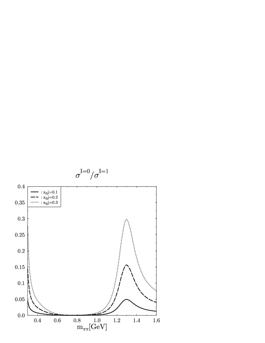
FIG. 3.: The ratio of the differential cross sections for isoscalar and isovector pion pair production at three different values for $x_{{\mathrm{B}j}}$ as a function of $m_{\pi\pi}$.

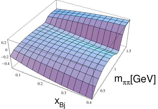
FIG. 4.: $\langle P_{1}(\cos\theta)\rangle^{\pi^{+}\pi^{-}}$ as a function of $x_{{\mathrm{B}j}}$ and $m_{\pi\pi}$.

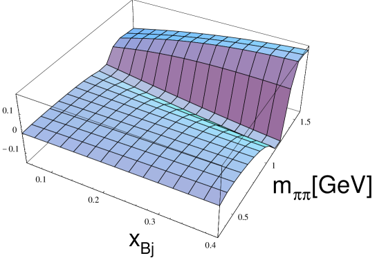
FIG. 5.: $\langle P_{3}(\cos\theta)\rangle^{\pi^{+}\pi^{-}}$ as a function of $x_{{\mathrm{B}j}}$ and $m_{\pi\pi}$.

FIG. 6.: $\langle P_{1}(\cos\theta)\rangle^{\pi^{+}\pi^{-}}+\sqrt{\frac{7}{3}}\langle P_{3}(\cos\theta)\rangle^{\pi^{+}\pi^{-}}$ as a function of $m_{\pi\pi}$ with cross sections integrated over $x_{{\mathrm{B}j}}$ from $0.05$ to $0.4$.

FIG. 7.: $\langle P_{1}(\cos\theta)\rangle^{\pi^{+}\pi^{-}}+\sqrt{\frac{7}{3}}\langle P_{3}(\cos\theta)\rangle^{\pi^{+}\pi^{-}}$ as a function of $x_{{\mathrm{B}j}}$ with cross sections integrated over $m_{\pi\pi}$ from the threshold to $0.6\,{\mathrm{G}eV}$. The dotted line shows the corresponding result obtained using the fit of [REFERENCES] instead of the Padé approximation for the Omnès function $f_{0}(m_{\pi\pi})$.

VII Summary

We have analyzed the angular distributions for exclusive electroproduction of pion pairs. Our analysis was based on the amplitudes at leading order in $1/Q^{2}$ and $\alpha_{{\mathrm{s}}}$. These amplitudes were expressed in terms of skewed parton distributions and two-pion distribution amplitudes, for which we have used realistic models. We have introduced intensity densities as Legendre moments of the two-pion angular distributions and we have shown that they are a good probe for the contribution of isoscalar pion pairs to the considered process. Our analytic results show that isoscalar pion pairs are mostly produced by two collinear gluons, which, in principle, opens a possibility to study the gluon content of the isoscalar $\pi\pi$ states. We predict sizable effects that could be measured at experiments like HERMES. As a promising kinematic range for a corresponding experiments we identified the $m_{\pi\pi}$-regions near the threshold and around the $f_{2}(1270)$ resonance and relatively large values of the Bjorken variable $x_{{\mathrm{B}j}}>0.2$. The $m_{\pi\pi}$-dependence should show a highly characteristic pattern. Our results are nearly parameter free such that experimental data would provide an excellent check for the whole formalism describing exclusive electroproduction processes with skewed parton distributions. In addition we have shown that studies of hard exclusive pion pair production near to the threshold open a new way to probe the effective chiral Lagrangian.

In this appendix are shown the full expressions for the $\cos\theta$-integrated absolute squares of the $T$-matrix elements, weighted with Legendre polynomials $P_{l}(\cos\theta)$, as they enter the intensity densities.

Using Eqs. (32) – (35), (43), and (44) we get

$$\int_{-1}^{1}{\mathrm{d}}\cos\theta\sum_{S^{\prime}}|T^{\pi^{+}\pi^{-}}|^{2} = \int_{-1}^{1}{\mathrm{d}}\cos\theta\sum_{S^{\prime}}\Bigl{(}|T^{I=0}|^{2}+|T^{I=1}|^{2}\Bigr{)}$$ (97)

$$\int_{-1}^{1}{\mathrm{d}}\cos\theta\sum_{S^{\prime}}|T^{\pi^{0}\pi^{0}}|^{2} = \int_{-1}^{1}{\mathrm{d}}\cos\theta\sum_{S^{\prime}}|T^{I=0}|^{2}$$ (98)

with

$$\int_{-1}^{1}{\mathrm{d}}\cos\theta\sum_{S^{\prime}}|T^{I=0}|^{2} = \frac{(e\pi\alpha_{{\mathrm{s}}})^{2}C_{F}^{2}}{18N_{c}^{2}}\frac{1}{p\cdot l\,x_{{\mathrm{B}j}}y}\sum_{S^{\prime}}\Bigl{|}2I_{u}^{-}-I_{d}^{-}\Bigr{|}^{2}\biggl{(}\frac{40M_{2}^{Q}}{N_{f}}+\frac{20M_{2}^{G}}{C_{F}}\biggr{)}^{2}$$ (100)

$$\times\Biggl{[}\frac{(3C-\beta^{2})^{2}}{72}|f_{0}(m_{\pi\pi})|^{2}+\frac{\beta^{4}}{90}|f_{2}(m_{\pi\pi})|^{2}\Biggr{]}$$

and

$$\int_{-1}^{1}{\mathrm{d}}\cos\theta\sum_{S^{\prime}}|T^{I=1}|^{2} = \frac{(e\pi\alpha_{{\mathrm{s}}})^{2}C_{F}^{2}}{18N_{c}^{2}}\frac{1}{p\cdot l\,x_{{\mathrm{B}j}}y}\sum_{S^{\prime}}\Bigl{|}2I_{u}^{+}+I_{d}^{+}+\frac{3}{C_{F}}I_{G}\Bigr{|}^{2}24\beta^{2}|F_{\pi}(m_{\pi\pi})|^{2}\,.$$ (101)

The other non-vanishing integrals are:

$$\int_{-1}^{1}{\mathrm{d}}\cos\theta\sum_{S^{\prime}}|T^{\pi^{+}\pi^{-}}|^{2}P_{1}(\cos\theta) = \frac{(e\pi\alpha_{{\mathrm{s}}})^{2}C_{F}^{2}}{18N_{c}^{2}}\frac{1}{p\cdot l\,x_{{\mathrm{B}j}}y}\biggl{(}\frac{40M_{2}^{Q}}{N_{f}}+\frac{20M_{2}^{G}}{C_{F}}\biggr{)}$$ (104)

$$\times 2{\mathrm{R}e}\Bigg{\{}\sum_{S^{\prime}}\Bigl{(}2I_{u}^{-}-I_{d}^{-}\Bigr{)}^{*}\Bigl{(}2I_{u}^{+}+I_{d}^{+}+\frac{3}{C_{F}}I_{G}\Bigr{)}$$

$$\qquad\times\Biggl{[}\frac{3C-\beta^{2}}{3}f_{0}(m_{\pi\pi})^{*}-\frac{4\beta^{2}}{15}f_{2}(m_{\pi\pi})^{*}\Biggr{]}\beta F_{\pi}(m_{\pi\pi})\Bigg{\}}$$

$$\int_{-1}^{1}{\mathrm{d}}\cos\theta\sum_{S^{\prime}}|T^{\pi^{+}\pi^{-}}|^{2}P_{2}(\cos\theta) = \frac{(e\pi\alpha_{{\mathrm{s}}})^{2}C_{F}^{2}}{18N_{c}^{2}}\frac{1}{p\cdot l\,x_{{\mathrm{B}j}}y}$$ (108)

$$\times\Biggl{\{}\sum_{S^{\prime}}\Bigl{|}2I_{u}^{-}-I_{d}^{-}\Bigr{|}^{2}\biggl{(}\frac{40M_{2}^{Q}}{N_{f}}+\frac{20M_{2}^{G}}{C_{F}}\biggr{)}^{2}$$

$$\qquad\times\Biggl{[}\frac{3C-\beta^{2}}{90}\beta^{2}{\mathrm{R}e}\Big{\{}f_{0}(m_{\pi\pi})^{*}f_{2}(m_{\pi\pi})\Big{\}}+\frac{\beta^{4}}{315}|f_{2}(m_{\pi\pi})|^{2}\Biggr{]}$$

$$\quad+\sum_{S^{\prime}}\Bigl{|}2I_{u}^{+}+I_{d}^{+}+\frac{3}{C_{F}}I_{G}\Bigr{|}^{2}\frac{144\beta^{2}}{35}|F_{\pi}(m_{\pi\pi})|^{2}\Biggr{\}}$$

$$\int_{-1}^{1}{\mathrm{d}}\cos\theta\sum_{S^{\prime}}|T^{\pi^{0}\pi^{0}}|^{2}P_{2}(\cos\theta) = \frac{(e\pi\alpha_{{\mathrm{s}}})^{2}C_{F}^{2}}{18N_{c}^{2}}\frac{1}{p\cdot l\,x_{{\mathrm{B}j}}y}\sum_{S^{\prime}}\Bigl{|}2I_{u}^{-}-I_{d}^{-}\Bigr{|}^{2}\biggl{(}\frac{40M_{2}^{Q}}{N_{f}}+\frac{20M_{2}^{G}}{C_{F}}\biggr{)}^{2}$$ (110)

$$\times\Biggl{[}\frac{3C-\beta^{2}}{90}\beta^{2}{\mathrm{R}e}\Big{\{}f_{0}(m_{\pi\pi})^{*}f_{2}(m_{\pi\pi})\Big{\}}+\frac{\beta^{4}}{315}|f_{2}(m_{\pi\pi})|^{2}\Biggr{]}$$

$$\int_{-1}^{1}{\mathrm{d}}\cos\theta\sum_{S^{\prime}}|T^{\pi^{+}\pi^{-}}|^{2}P_{3}(\cos\theta) = -\frac{(e\pi\alpha_{{\mathrm{s}}})^{2}C_{F}^{2}}{18N_{c}^{2}}\frac{1}{p\cdot l\,x_{{\mathrm{B}j}}y}\biggl{(}\frac{40M_{2}^{Q}}{N_{f}}+\frac{20M_{2}^{G}}{C_{F}}\biggr{)}$$ (112)

$$\times 2{\mathrm{R}e}\Bigg{\{}\sum_{S^{\prime}}\Bigl{(}2I_{u}^{-}-I_{d}^{-}\Bigr{)}^{*}\Bigl{(}2I_{u}^{+}+I_{d}^{+}+\frac{3}{C_{F}}I_{G}\Bigr{)}\frac{6\beta^{3}}{35}f_{2}(m_{\pi\pi})^{*}F_{\pi}(m_{\pi\pi})\Bigg{\}}$$

$$\int_{-1}^{1}{\mathrm{d}}\cos\theta\sum_{S^{\prime}}|T^{\pi^{+}\pi^{-}}|^{2}P_{4}(\cos\theta) = \int_{-1}^{1}{\mathrm{d}}\cos\theta\sum_{S^{\prime}}|T^{\pi^{0}\pi^{0}}|^{2}P_{4}(\cos\theta)$$ (113)

$$= \frac{(e\pi\alpha_{{\mathrm{s}}})^{2}C_{F}^{2}}{18N_{c}^{2}}\frac{1}{p\cdot l\,x_{{\mathrm{B}j}}y}\sum_{S^{\prime}}\Bigl{|}2I_{u}^{-}-I_{d}^{-}\Bigr{|}^{2}\biggl{(}\frac{40M_{2}^{Q}}{N_{f}}+\frac{20M_{2}^{G}}{C_{F}}\biggr{)}^{2}\frac{\beta^{4}}{315}|f_{2}(m_{\pi\pi})|^{2}\,.$$ (114)

REFERENCES

• [1] J. Collins, L. Frankfurt, and M. Strikman, Phys. Rev. D 56, 2982 (1997).
• [2] D. Müller et al., Fort. Phys. 42, 101 (1994).
• [3] X. Ji, Phys. Rev. D 55, 7114 (1997).
• [4] A. V. Radyushkin, Phys. Rev. D 56, 5524 (1997).
• [5] X. Ji, J. Phys. G 24, 1181 (1998).
• [6] A. V. Belitsky and A. Schäfer, Nucl. Phys. B 527, 235 (1998); M. Vänttinen, L. Mankiewicz, and E. Stein, Higher-twist contributions in exclusive processes, hep-ph/9810527; M. Vanderhaeghen, P. A. M. Guichon, and M. Guidal, Phys. Rev. D 60, 094017 (1999).
• [7] S. J. Brodsky, L. Frankfurt, J. F. Gunion, A. H. Mueller, and M. Strikman, Phys. Rev. D 50, 3134 (1994).
• [8] A. V. Radyushkin, Phys. Lett. B 385, 333 (1996).
• [9] L. Mankiewicz, G. Piller, and T. Weigl, Eur. Phys. J. C 5, 119 (1998); Phys. Rev. D 59, 017501 (1999).
• [10] M. Vanderhaeghen, P. A. M. Guichon, and M. Guidal, Phys. Rev. Lett. 80, 5064 (1998).
• [11] A. Freund, Phys. Rev. D 61, 074010 (2000).
• [12] B. Clerbaux and M. V. Polyakov, Nucl. Phys. A 679, 185 (2000).
• [13] B. Lehmann-Dronke, P. V. Pobylitsa, M. V. Polyakov, A. Schäfer, and K. Goeke, Phys. Lett. B 475, 147 (2000).
• [14] M. Diehl, T. Gousset, and B. Pire, Polarisation in deeply virtual meson production, hep-ph/9909445.
• [15] P. Minkowski and W. Ochs, The $J^{PC}=0^{++}$ Scalar Meson Nonet and Glueball of Lowest Mass, hep-ph/9905250.
• [16] S. Narison, On the Quark and Gluon Substructure of the $\sigma$ and other Scalar Mesons, hep-ph/0009108.
• [17] M. V. Polyakov, Nucl. Phys. B 555, 231 (1999).
• [18] R. L. Sekulin, Nucl. Phys. B 56, 227 (1973).
• [19] B. R. Martin, D. Morgan, and G. Shaw, Pion–Pion Interactions in Particle Physics, Academic Press, London (1976).
• [20] M. Diehl, T. Gousset, B. Pire, and O. V. Teryaev, Phys. Rev. Lett. 81, 1782 (1998).
• [21] N. Kivel, L. Mankiewicz, and M. V. Polyakov, Phys. Lett. B 467, 263 (1999).
• [22] G. P. Lepage and S. J. Brodsky, Phys. Lett. B 87, 359 (1979); A. V. Efremov and A. V. Radyushkin, Phys. Lett. B 94, 245 (1980).
• [23] M. K. Chase, Nucl. Phys. B 174, 109 (1980); Th. Ohrndorf, Nucl. Phys. B 186, 153 (1981); V. N. Baier and A. G. Grozin, Nucl. Phys. B 192, 476 (1981).
• [24] M. V. Polyakov and C. Weiss, Phys. Rev. D 59, 091502 (1999).
• [25] S. Raby and G. B. West, Phys. Rev. D 38, 3488 (1988).
• [26] J. F. Donoghue, J. Gasser, and H. Leutwyler, Nucl. Phys. B 343, 341 (1990).
• [27] K. M. Watson, Phys. Rev. 95, 228 (1954).
• [28] R. Omnès, Nuovo Cim. 8, 316 (1958).
• [29] A. V. Radyushkin, Phys. Rev. D 59, 014030 (1999).
• [30] A. D. Martin, R. G. Roberts, and W. J. Stirling, Phys. Lett. B 354, 155 (1995).
• [31] A. V. Belitsky, B. Geyer, D. Müller, and A. Schäfer, Phys. Lett. B 421, 312 (1998); A. V. Belitsky, D. Müller, L.  Niedermeier, and A. Schäfer, Phys. Lett. B 437, 160 (1998); Nucl. Phys. B 546, 279 (1999).
• [32] T. Ericson and W. Weise, Pions and Nuclei, Oxford University Press, (1988).
• [33] V. M. Braun, P. Gornicki, L. Mankiewicz, and A. Schäfer, Phys. Lett. B 302, 291 (1993).
• [34] M. V. Polyakov and C. Weiss, Phys. Rev. D 60, 114017 (1999).
• [35] V. Y. Petrov, P. V. Pobylitsa, M. V. Polyakov, I. Bornig, K. Goeke, and C. Weiss, Phys. Rev. D 57, 4325 (1998).
• [36] J. Gasser and H. Leutwyler, Nucl. Phys. B 250, 465 (1985).
• [37] J. F. Donoghue and H. Leutwyler, Z. Phys. C 52, 343 (1991).
• [38] J. Gasser, H. Leutwyler, Nucl. Phys. B 250, 517 (1985).
• [39] A. G. Nicola, Nonequilibrium Chiral Perturbation Theory and Disoriented Chiral Condensates, hep-ph/9910533.
• [40] B. Kubis and U.-G. Meißner, Nucl. Phys. A 671, 332 (2000).
• [41] N. Kivel and L. Mankiewicz, Power Corrections to the Process $\gamma\gamma^{*}\to\pi\pi$ in the Light-Cone Sum Rules Approach, hep-ph/0008168.
• [42] F. Guerrero and A. Pich, Phys. Lett. B 412, 382 (1997).
• [43] L. M. Barkov et al., Nucl. Phys. B 256, 365 (1985); S. D. Protopopescu et al., Phys. Rev. D 7, 1279 (1973).
• [44] J. F. Donoghue and B. R. Holstein, Phys. Rev. D 48, 137 (1993).
• [45] K. Ackerstaff et al., Nucl. Instrum. Meth. A 417, 230 (1998).
• [46] L. Mankiewicz, G. Piller, E. Stein, M. Vänttinen, and T. Weigl, Phys. Lett. B 425, 186 (1998); A. V. Belitsky, D. Müller, L. Niedermeier, and A. Schäfer, Phys. Lett. B 474, 163 (2000).