Bounds on Universal Extra Dimensions

We show that the bound from the electroweak data on the size of extra dimensions accessible to all the standard model fields is rather loose. These “universal” extra dimensions could have a compactification scale as low as 300 GeV for one extra dimension. This is because the Kaluza-Klein number is conserved and thus the contributions to the electroweak observables arise only from loops. The main constraint comes from weak-isospin violation effects. We also compute the contributions to the $S$ parameter and the $Zb\bar{b}$ vertex. The direct bound on the compactification scale is set by CDF and D0 in the few hundred GeV range, and the Run II of the Tevatron will either discover extra dimensions or else it could significantly raise the bound on the compactification scale. In the case of two universal extra dimensions, the current lower bound on the compactification scale depends logarithmically on the ultra-violet cutoff of the higher dimensional theory, but can be estimated to lie between 400 and 800 GeV. With three or more extra dimensions, the cutoff dependence may be too strong to allow an estimate.

1 Introduction

Extra dimensions accessible to standard model fields are of interest for various reasons. They could allow gauge coupling unification [1], and provide new mechanisms for supersymmetry breaking [2] and the generation of fermion mass hierarchies [3]. More recently it has been shown that extra dimensions accessible to the observed fields may lead to the existence of a Higgs doublet [4].

A number of studies indicate that if standard model fields propagate in extra dimensions, then they must be compactified at a scale $1/R$ above a few TeV [5]. These studies refer, however, to theories in which some of the quarks and leptons are confined to flat four-dimensional slices (branes). In the equivalent four-dimensional theory where the extra dimensions are accounted for by towers of heavy Kaluza-Klein (KK) states, the bound on $1/R$ is due to the tree level contributions of the KK modes to the electroweak observables.

In this paper we point out that extra dimensions accessible to all the standard model fields, referred to here as universal dimensions, may be significantly larger. The key element is the conservation of momentum in the universal dimensions. In the equivalent four-dimensional theory this implies KK number conservation. In particular there are no vertices involving only one non-zero KK mode, and consequently there are no tree-level contributions to the electroweak observables. Furthermore, non-zero KK modes may be produced at colliders only in groups of two or more. Thus, none of the known bounds on extra dimensions from single KK production at colliders or from electroweak constraints applies for universal extra dimensions.

The heavy KK modes contribute, though, at loop-level to the electroweak observables, so that some lower bound on $1/R$ can be set. In addition, there is a direct bound on $1/R$ from the non-observation of KK pair production at the Tevatron and LEP. After presenting some general features of universal extra dimensions in section 2, we compute the bound on their size from the electroweak data (section 3.) We then discuss the current direct bound on $1/R$ from collider experiments (section 4.) Our conclusions are summarized in section 5.

2 The Kaluza-Klein spectrum and interactions

Our starting point is the minimal standard model in $d=4+\delta$ space-time dimensions. The gauge, Yukawa and quartic-Higgs couplings have negative mass dimension, so this is an effective theory, valid below some scale $M_{s}$. We assume a compactification scale $1/R<M_{s}$ for the $\delta$ extra spatial dimensions. The upper bound on $1/R$ for the class of models being discussed is determined by the range of validity of the effective 4-dimensional Higgs theory. To avoid fine-tuning the parameters in the Higgs sector, $1/R$ should not be much higher than the electroweak scale. We study the experimental lower bound on $1/R$. Given that the gauge couplings and the top Yukawa coupling are of order one at the electroweak scale, the $d$-dimensional theory remains perturbative for a range of energies above $1/R$. The cutoff $M_{s}$ on the $d$-dimensional theory is expected to be no higher than the upper end of this range.

We use the generic notation $x^{\alpha},\;\alpha=0,1,...,3+\delta$ for the coordinates of the $(4+\delta)$-dimensional space-time, but we explicitly distinguish between the usual non-compact space-time coordinates, $x^{\mu},\,\mu=0,1,2,3$, and the coordinates of the extra dimensions, $y^{a},\,a=1,...,\delta$. The 4-dimensional Lagrangian can be obtained by dimensional reduction from the $(4+\delta)$-dimensional theory,

$${\cal L}(x^{\mu}) = \int d^{\delta}y\left\{-\sum_{i=1}^{3}\frac{1}{2\hat{g}_{i}^{2}}{\rm Tr}\left[F_{i}^{\alpha\beta}(x^{\mu},y^{a}){F_{i}}_{\,\alpha\beta}(x^{\mu},y^{a})\right]+{\cal L}_{\rm Higgs}(x^{\mu},y^{a})\right.$$ (2.1)

$$+ \left.\!\!\!\!i\left(\overline{{\cal Q}},\overline{{\cal U}},\overline{{\cal D}}\right)(x^{\mu},y^{a})\left(\Gamma^{\mu}D_{\mu}+\Gamma^{3+a}D_{3+a}\right)\left({\cal Q},{\cal U},{\cal D}\right)^{\top}(x^{\mu},y^{a})\right.$$

$$+ \left.\!\!\!\!\!\left[\overline{{\cal Q}}(x^{\mu},y^{a})\left(\hat{\lambda}_{\cal U}{\cal U}(x^{\mu},y^{a})i\sigma_{2}H^{*}(x^{\mu},y^{a})+\hat{\lambda}_{\cal D}{\cal D}(x^{\mu},y^{a})H(x^{\mu},y^{a})\right)+{\rm h.c.}\right]\right\}~{}.$$

Here $F^{\alpha\beta}_{i}$ are the $(4+\delta)$-dimensional gauge field strengths associated with the $SU(3)_{C}\times SU(2)_{W}\times U(1)_{Y}$ group, while $D_{\mu}=\partial/\partial x^{\mu}-{\cal A}_{\mu}$ and $D_{3+a}=\partial/\partial y^{a}-{\cal A}_{3+a}$ are the covariant derivatives, with ${\cal A}_{\alpha}=-i\sum_{i=1}^{3}\hat{g}_{i}{{\cal A}_{\alpha}^{r}}_{i}T^{r}_{i}$ being the $(4+\delta)$-dimensional gauge fields. The piece ${\cal L}_{\rm Higgs}$ of the $(4+\delta)$-dimensional Lagrangian contains the kinetic term for the $(4+\delta)$-dimensional Higgs doublet $H$, and the Higgs potential. The $(4+\delta)$-dimensional gauge couplings $\hat{g}_{i}$, and the Yukawa couplings collected in the $3\times 3$ matrices $\hat{\lambda}_{{\cal U},{\cal D}}$, have dimension (mass)^-δ/2.

The fields ${\cal Q},{\cal U}$ and ${\cal D}$ describe the $(4+\delta)$-dimensional fermions whose zero-modes are given by the 4-dimensional standard model quarks. A summation over a generational index is implicit in Eq. (2.1). For example, the 4-dimensional, third generation quarks may be written as ${\cal Q}^{(0)}_{3}\equiv(t,b)_{L},\,{\cal U}^{(0)}_{3}\equiv t_{R},\,{\cal D}^{(0)}_{3}\equiv b_{R}$. The kinetic and Yukawa terms for the weak-doublet and -singlet leptons, ${\cal L}$ and ${\cal E}$, are not shown for brevity.

The gamma matrices in $(4+\delta)$ dimensions, $\Gamma^{\alpha}$, are anti-commuting $2^{k+2}\times 2^{k+2}$ matrices, where $k$ is an integer such that $\delta=2k$ or $\delta=2k+1$. Chiral fermions exist only when $\delta$ is even, and correspond to the eigenvalues $\pm 1$ of $\Gamma^{4+\delta}$. Therefore, if the spacetime has an odd number of dimensions ($\delta=2k+1$), ${\cal Q},{\cal U},{\cal D},{\cal L},$ and ${\cal E}$ are vector-like $2^{k+2}$-component fermions, and the $(4+\delta)$-dimensional theory is automatically anomaly-free. For an even number of dimensions ($\delta=2k$) one may choose ${\cal Q},{\cal U},{\cal D},{\cal L}$ and ${\cal E}$ to be chiral $2^{k+1}$-component fermions. In order to have Yukawa couplings with the scalar Higgs field, the $SU(2)_{W}$-doublet fermions and the $SU(2)_{W}$-singlet fermions must have opposite chiralities. This guarantees that the unbroken $SU(3)_{C}$ and $U(1)_{\rm EM}$ are vector-like, hence anomaly free. The gravitational anomaly may easily be cancelled by gauge-singlet fermions. The $SU(2)_{W}$ and $U(1)_{Y}$ gauge groups are chiral, so there can be $(4+2k)$-dimensional anomalies involving the $SU(2)_{W}$ and $U(1)_{Y}$ gauge groups, but they can be cancelled by the Green-Schwarz mechanism [6]. For both odd and even $\delta$ the 4-dimensional anomalies cancel because the fermion content is chosen so that the effective theory at scales below $1/R$ is the 4-dimensional standard model.

In order to derive the 4-dimensional Lagrangian from Eq. (2.1), we must specify the compactification of the extra dimensions. The simplest choice is an $[(S^{1}\times S^{1})/Z_{2}]^{k}$ orbifold for $\delta=2k$, and an $[(S^{1}\times S^{1})/Z_{2}]^{k}\times(S^{1}/Z_{2})$ orbifold for $\delta=2k+1$. An orbifold of this type is a $\delta$-dimensional torus cut in half along each of the $y^{a}$ coordinates with odd $a$. Each component of a $d$-dimensional field that belongs to a representation of the 4-dimensional Lorentz group, $SO(3,1)$, must be either odd or even under the orbifold projection: $(y^{a},\,y^{a+1})\rightarrow(-y^{a},\,-y^{a+1})$ for even $a+1\leq 2k$, as well as $y^{2k+1}\rightarrow-y^{2k+1}$ for $\delta=2k+1$. An equivalent description of the compactification is a $\delta$-dimensional space with coordinates $0\leq y^{a}\leq\pi R$ for odd $a$ and $-\pi R\leq y^{a}\leq\pi R$ for even $a$, and boundary conditions such that each field or its derivatives with respect to the $y^{a}$’s vanish at the orbifold fixed points $y^{a}=0,\,\pm\pi R$. ($\Phi=0,\,\partial^{2}\Phi/\partial y^{a}\partial y^{b}=0$ for odd fields, and $\partial\Phi/\partial y^{a}=0$ for even fields at the orbifold fixed points.)

The Lagrangian (2.1) together with the boundary conditions completely specifies the theory. For $\delta=2$, the $SU(3)_{C}\times SU(2)_{W}\times U(1)_{Y}$ gauge fields are decomposed in KK modes as follows:

$${\cal A}_{\nu}(x^{\mu},y^{a}) = \frac{\sqrt{2}}{(2\pi R)^{\delta/2}}\left\{{\cal A}_{\nu}^{(0,0)}(x^{\mu})_{\begin{array}[]{c}\\ \end{array}}\right.+\sqrt{2}\sum_{j_{1},j_{2}}\left.{\cal A}_{\nu}^{(j_{1},j_{2})}(x^{\mu})_{\begin{array}[]{c}\\ \end{array}}\!\!\!\!\cos\left[\frac{1}{R}(j_{1}y^{1}+j_{2}y^{2})\right]\right\}~{},$$ (2.4)

$${\cal A}_{b}(x^{\mu},y^{a}) = \frac{2}{(2\pi R)^{\delta/2}}\sum_{j_{1},j_{2}}{\cal A}_{b}^{(j_{1},j_{2})}(x^{\mu})\,\sin\left[\frac{1}{R}(j_{1}y^{1}+j_{2}y^{2})\right]~{},$$ (2.5)

where the summation is over all integer values of the KK numbers $j_{1}$ and $j_{2}$ that satisfy $j_{1}+j_{2}\geq 1$, or $j_{1}=-j_{2}\geq 1$. The gauge fields polarized in the $x^{\nu},\,\nu=0,1,2,3$ directions are even under the orbifold transformation, so that the zero-modes correspond to the 4-dimensional standard model gauge fields. On the other hand, the gauge fields polarized along the coordinates $y^{b},\,b=1,2$ of the extra dimensions are odd under the orbifold transformation, so that their zero-modes are projected out and no massless scalar fields appear after dimensional reduction.

With boundary conditions in the $\delta=2$ compact dimensions chosen to give the appropriate chiral structure for the KK zero-modes, the KK decomposition for the top quark fields is given by

$${\cal Q}_{3}(x^{\mu},y^{a}) = \frac{\sqrt{2}}{(2\pi R)^{\delta/2}}\left\{(t,b)_{L}(x^{\mu})_{\begin{array}[]{c}\\ \end{array}}\right.+\sqrt{2}\sum_{j_{1},j_{2}}\left[P_{L}{{\cal Q}_{3}}_{L}^{(j_{1},j_{2})}(x^{\mu})\,\cos\left(\frac{1}{R}(j_{1}y^{1}+j_{2}y^{2})\right)\right.$$

$$+\left.\left.P_{R}{{\cal Q}_{3}}_{R}^{(j_{1},j_{2})}(x^{\mu})\,\sin\left(\frac{1}{R}(j_{1}y^{1}+j_{2}y^{2})\right)\right]\right\}~{},$$

$${\cal U}_{3}(x^{\mu},y^{a}) = \frac{\sqrt{2}}{(2\pi R)^{\delta/2}}\left\{t_{R}(x^{\mu})_{\begin{array}[]{c}\\ \end{array}}\right.+\sqrt{2}\sum_{j_{1},j_{2}}\left[P_{R}{{\cal U}_{3}}_{R}^{(j_{1},j_{2})}(x^{\mu})\,\cos\left(\frac{1}{R}(j_{1}y^{1}+j_{2}y^{2})\right)\right.$$ (2.10)

$$+\left.\left.P_{L}{{\cal U}_{3}}_{L}^{(j_{1},j_{2})}(x^{\mu})\,\sin\left(\frac{1}{R}(j_{1}y^{1}+j_{2}y^{2})\right)\right]\right\}~{},$$

where the range of values for $j_{1}$ and $j_{2}$ is the same as above, in Eq. (2.5). The third-generation weak-doublet quark, ${\cal Q}_{3}=({\cal Q}_{t},{\cal Q}_{b})$, and weak-singlet up-type quark, ${\cal U}_{3}$, are four-component chiral fermions in six dimensions so that their KK modes are 4-dimensional vector-like quarks, with the exception of the zero-modes which are chiral. The chiral projection operators that appear in the KK decomposition, $P_{L,R}=(1\mp\gamma_{5})/2$, are the 4-dimensional ones.

For $\delta=1$, the KK decomposition may be obtained from Eqs. (2.5) and (2.10) by setting $j_{2}=0,\,y^{2}=0$. In general, for $\delta=2k+1$ one may compactify one dimension as above and then compactify the remaining $k$ pairs of extra dimensions, with appropriate use of the higher dimensional chiral projection operators. For $\delta=2k$, the KK decomposition may also be obtained by iterating Eqs. (2.5) and (2.10) $k$ times. The other quark and lepton $d$-dimensional fields have similar KK-mode decompositions. The Higgs field must be even under the orbifold transformation. Only the Higgs zero-mode acquires an electroweak asymmetric vacuum expectation value (VEV) of $v/\sqrt{2}\approx 174$ GeV.

The heavy spectrum in four dimensions consists of KK levels characterized by the mass eigenvalues

$$M_{j}=\frac{p_{j}}{R}~{},$$ (2.11)

where $j\geq 1$, $p_{j+1}>p_{j}$, and $p_{j}$ is given by

$$j_{1}^{2}+...+j_{\delta}^{2}=p_{j}^{2}~{}.$$ (2.12)

The degeneracy of the $j$th KK level, $D_{j}$, is given by the number of solutions to this equation for $j_{1},...,j_{\delta}$. At each level there would be $D_{j}$ sets of fields, each of them including the $SU(3)_{C}\times SU(2)_{W}\times U(1)_{Y}$ gauge fields, three generations of vector-like quarks and leptons, a Higgs doublet, and $\delta$ scalars in the adjoint representations of $SU(3)_{C}\times SU(2)_{W}\times U(1)_{Y}$.

An essential observation is that the momentum conservation in the extra dimensions, implicitly associated with the Lagrangian (2.1), is preserved (as a discrete symmetry) by the above orbifold projection. In the case of fermions, this implies that there is no mixing among the modes of different KK levels. The zero-mode top-quark gets a mass from its Yukawa coupling exactly as in the 4-dimensional standard model. Given that each KK level includes a tower of both left- and right-handed modes for each of the $t_{L}$ and $t_{R}$ fields, there is a $2\times 2$ mass matrix for each top-quark KK level. The $D_{j}$ top-quark mass matrices of the $j$th KK level may be written in the weak eigenstate basis as

$$\left(\overline{{\cal U}}_{3}^{j},\overline{{\cal Q}}_{t}^{j}\right)\left(\begin{array}[]{c c}-M_{j}&m_{t}\\ m_{t}&M_{j}\end{array}\right)\left(\begin{array}[]{c}{\cal U}^{j}_{3}\\ {\cal Q}_{t}^{j}\end{array}\right)~{}.$$ (2.13)

Here, ${\cal Q}_{t}^{j}$ is a four-component field describing the $j$th KK modes associated with $t_{L}$. The diagonal terms are the masses induced by the kinetic terms in the $y^{a}$ directions, while the off-diagonal terms are the contributions from the Higgs VEV. The corresponding mass eigenstates, ${\cal U}_{3}^{\prime j}$ and ${\cal Q}_{t}^{\prime j}$, have the same mass,

$$M^{(j)}_{t}=\sqrt{M_{j}^{2}+m_{t}^{2}}~{}.$$ (2.14)

The weak eigenstate top KK modes are related to the mass eigenstates by

$$\left(\begin{array}[]{c}{\cal U}^{j}_{3}\\ {\cal Q}_{t}^{j}\end{array}\right)=\left(\begin{array}[]{c c}-\gamma_{5}\cos\alpha_{j}&\sin\alpha_{j}\\ \gamma_{5}\sin\alpha_{j}&\cos\alpha_{j}\end{array}\right)\left(\begin{array}[]{c}{\cal U}^{\prime j}_{3}\\ {\cal Q}^{\prime j}_{t}\end{array}\right)~{},$$ (2.15)

where $\alpha_{j}$ is the mixing angle,

$$\tan 2\alpha_{j}=\frac{m_{t}}{M_{j}}~{}.$$ (2.16)

The $b$-quark KK modes have an analogous structure due to the mixing between ${\cal D}_{3}^{j}$ (the left- and right-handed fields associated with $b_{R}$) and ${\cal Q}_{b}^{j}$ (the left- and right-handed fields associated with $b_{L}$). However, this mixing may be neglected up to corrections of order $(m_{b}/m_{t})^{2}$ compared with the mixing from the top-quark KK sector.

The interactions of the KK modes may be derived from the $d$-dimensional Lagrangian (2.1), using the KK decompositions shown in Eqs. (2.5) and (2.10), and by integrating over the extra dimensions. For the one-loop computations to be considered here, it is sufficient to know the vertices involving one or two zero-modes and two non-zero modes. In the remainder of this section we list the relevant terms of this type that appear in the 4-dimensional Lagrangian.

The top and bottom mass-eigenstate KK modes (i.e., the vector-like quarks ${\cal Q}_{t}^{\prime j},\,{\cal U}_{3}^{\prime j}$, ${\cal Q}_{b}^{j}$ and ${\cal D}_{3}^{j}$) have the following electroweak interactions with the $W^{\pm}$ and $Z$ zero-modes:

$${\cal L}_{W_{1}} = \frac{g}{2\cos\theta_{W}}Z_{\mu}\left[\left(\sin^{2}\alpha_{j}-\frac{4}{3}\sin^{2}\theta_{W}\right)\overline{{\cal U}}_{3}^{\prime j}\gamma^{\mu}{\cal U}_{3}^{\prime j}+\left(\cos^{2}\alpha_{j}-\frac{4}{3}\sin^{2}\theta_{W}\right)\overline{{\cal Q}}_{t}^{\prime j}\gamma^{\mu}{\cal Q}_{t}^{\prime j}\right.$$ (2.17)

$$\left.+\sin\alpha_{j}\cos\alpha_{j}\left(\overline{{\cal U}}_{3}^{\prime j}\gamma^{\mu}\gamma_{5}{\cal Q}_{t}^{\prime j}+{\rm h.c.}\right)+2g_{L}^{b}\overline{{\cal Q}}_{b}^{j}\gamma^{\mu}{\cal Q}_{b}^{j}+2g_{R}^{b}\overline{{\cal D}}_{3}^{j}\gamma^{\mu}{\cal D}_{3}^{j}\right]$$

$$+ \frac{g}{\sqrt{2}}\left[W^{+}_{\mu}\left(-\sin\alpha_{j}\overline{{\cal U}}_{3}^{\prime j}\gamma_{5}+\cos\alpha_{j}\overline{{\cal Q}}_{t}^{\prime j}\right)\gamma^{\mu}{\cal Q}_{b}^{j}+{\rm h.c.}\right]~{},$$

where

$$g_{L}^{b}=-\frac{1}{2}+\frac{1}{3}\sin^{2}\theta_{W}\;,\;\;g_{R}^{b}=\frac{1}{3}\sin^{2}\theta_{W}~{}.$$ (2.18)

The weak eigenstate neutral gauge bosons, ${W^{3}_{\mu}}^{j}$ and $B^{j}_{\mu}$ mix level by level in the same way as the neutral $SU(2)_{W}$ and hypercharge gauge bosons in the 4-dimensional standard model. The corresponding mass eigenstates, $Z_{\mu}^{j}$ and $A^{j}_{\mu}$, have masses $\sqrt{M_{j}^{2}+M_{Z}^{2}}$ and $M_{j}^{2}$, respectively. These heavy gauge bosons have interactions with one zero-mode quark and one $j$-mode quark (in the weak-eigenstate basis) identical with the standard model interactions of the zero-modes.

Likewise, there are interactions of one quark zero-mode and one quark $j$-mode with the $j$-mode of the scalars corresponding to the electroweak gauge bosons polarized along $y^{a}$, $W_{a+3}^{j},\,Z_{a+3}^{j},\,A_{a+3}^{j}$. For $\delta=1$, they may be written as follows:

$${\cal L}_{W_{2}} = \frac{e}{3}iA_{4}^{j}\left[2\cos\alpha_{j}\left(\overline{{\cal Q}}_{t_{R}}^{\prime j}t_{L}-\overline{{\cal U}}_{3_{L}}^{\prime j}t_{R}\right)-2\sin\alpha_{j}\left(\overline{{\cal U}}_{3_{R}}^{\prime j}t_{L}-\overline{{\cal Q}}_{t_{L}}^{\prime j}t_{R}\right)-\overline{{\cal Q}}_{b_{R}}^{j}b_{L}-\overline{{\cal D}}_{3_{L}}^{j}b_{R}\right]$$ (2.19)

$$+ \frac{g}{\cos\theta_{W}}iZ_{4}^{j}\left[\overline{{\cal Q}}_{t}^{\prime j}\left(c^{j}_{1_{V}}+c_{1_{A}}^{j}\gamma_{5}\right)t+\overline{{\cal U}}_{3}^{\prime j}\left(c_{2_{V}}^{j}+c_{2_{A}}^{j}\gamma_{5}\right)t+g_{L}^{b}{\cal Q}_{b_{R}}^{j}b_{L}+g_{R}^{b}\overline{{\cal D}}_{3_{L}}^{j}b_{R}\right]$$

$$+ \frac{g}{\sqrt{2}}i{W^{+}_{4}}^{j}\left(\cos\alpha_{j}\overline{{\cal Q}}_{t_{R}}^{\prime j}b_{L}-\sin\alpha_{j}\overline{{\cal U}}_{3_{R}}^{\prime j}b_{L}+\overline{t}_{L}{\cal Q}_{b_{R}}^{j}\right)+{\rm h.c.}$$

where

$$c_{1_{V,A}}^{j}=\pm\cos\alpha_{j}\left(\frac{1}{4}-\frac{1}{3}\sin^{2}\theta_{W}\right)-\frac{1}{3}\sin\alpha_{j}\sin^{2}\theta_{W}~{},$$ (2.20)

and $c_{2_{V,A}}^{j}$ are obtained by permuting $\sin\alpha_{j}$ and $\cos\alpha_{j}$ in the above expression. For $\delta=2$ the $W_{a+4}^{j},\,Z_{a+4}^{j},\,\gamma_{a+4}^{j}$ scalars have similar couplings, up to sign differences, while for $\delta\geq 3$ the gauge bosons polarized along each pair of extra dimensions couples to a different set of quark KK modes.

Each non-zero KK mode of the Higgs doublet, $H^{j}$, includes a charged Higgs and a neutral CP-odd scalar of mass $M_{j}$, and also a neutral CP-even scalar of mass $\sqrt{M_{j}^{2}+M_{h}^{2}}$. The interactions of the Higgs and gauge boson KK modes may also be obtained from the corresponding standard model interactions of the zero-modes by replacing two of the fields at each vertex with their $j$th KK mode.

3 Electroweak data versus extra dimensions

We study the sensitivity of the electroweak observables to the higher dimensional physics setting in at scale $1/R$. The largest contributions come from the KK modes associated with the top-quark, but there are also corrections due to the gauge and Higgs KK modes. QCD corrections are small and are neglected. The standard model in universal extra dimensions is described by four unknown parameters: the Higgs boson mass $M_{h}$, the compactification radius $R$, the cutoff scale $M_{s}$, and the number of extra dimensions $\delta$. The upper bound on the cutoff $M_{s}$ is determined in terms of $1/R$ and the value of the various couplings at this scale. The Higgs boson mass is bounded from above by the requirement that the Higgs quartic coupling, $\lambda_{h}$, does not blow up (from a perturbative point of view) at a scale significantly below $M_{s}$. We use this constraint ($M_{h}\begin{array}[]{c}\,\sim\vspace{-21pt}\\ <\end{array}250$ GeV [4]), and study the lower bound on $1/R$, concentrating on the observables that are most likely to yield severe constraints.

An important question is whether the electroweak observables can be computed within the framework of the effective, higher dimensional theory, that is, whether they are sensitive to the unknown physics at scale $M_{s}$ and above. We will show that in the case of one extra dimension we can reliably ignore the effects of KK modes heavier than the cut-off (see section 3.1). With two extra dimensions the KK modes give corrections to the electroweak observables that depend logarithmically on the cut-off, and in more extra dimensions the dependence is more sensitive (see section 3.2).

Given that the large $t-b$ mass splitting requires a hierarchy between the top and bottom Yukawa couplings which in turn induces weak isospin violation in the KK spectrum, the parameter

$$\Delta\rho\equiv\alpha T=\Delta\left(\frac{M_{W}}{M_{Z}\cos\theta_{W}}\right),$$ (3.1)

which measures the splitting in the $W$ and $Z$ masses due to physics beyond the standard model, is a prime suspect for constraining $1/R$.

The one-loop contribution to $\Delta\rho$ from one KK level associated with the $t$ and $b$ quarks follows from Eq. (2.17) and is given by

$$\alpha T_{j}^{t}=\frac{3m_{t}^{2}}{16\pi^{2}v^{2}}f_{T}\left(m_{t}^{2}/M_{j}^{2}\right)~{},$$ (3.2)

where $v=246$ GeV and

$$f_{T}(z) = 1-\frac{2}{z}+\frac{2}{z^{2}}\ln\left(1+z\right)$$ (3.3)

$$= \frac{2z}{3}\left[1-\frac{3z}{4}+\frac{3z^{2}}{5}+{\cal O}\left(z^{3}\right)\right]~{}.$$

The form of this contribution to $\Delta\rho$ is easy to understand. The factor $m_{t}^{2}/(4\pi v)^{2}$ arises from the definition of $\Delta\rho$ as the coefficient of the lowest-dimension, weak isospin-violating term in the electroweak chiral Lagrangian [8]. The additional factor $(m_{t}^{2}/M_{j}^{2})$ is present because the non-zero KK modes decouple in the large mass limit.

In addition to the top and bottom KK modes, the Higgs KK modes contribute to $\Delta\rho$ because the VEV of the zero-mode Higgs induces isospin violation in the couplings of the higher modes of the Higgs doublet. To leading order in $M_{h}^{2}/M_{j}^{2}$, one Higgs KK mode gives

$$\alpha T^{h}_{j}=-\left(\frac{\alpha}{4\pi\cos^{2}\theta_{W}}\right)\frac{5M_{h}^{2}+7M_{W}^{2}}{12M_{j}^{2}}$$ (3.4)

Finally, the KK electroweak gauge bosons also contribute, giving

$$\alpha T_{j}^{V}=-\left(\frac{\alpha}{4\pi\cos^{2}\theta_{W}}\right)\frac{(2\delta+11)M_{W}^{2}}{6M_{j}^{2}}~{}.$$ (3.5)

In each of these expressions, the factor $\alpha/\cos^{2}\theta_{W}$ is present because the hypercharge gauge interaction provides the weak-isospin symmetry breaking. The second factor is present because the higher KK modes decouple in the large mass limit.

The contribution to $T$ from all the KK modes is

$$T=\sum_{j=1}^{n_{\rm max}}D_{j}\left(T_{j}^{t}+T_{j}^{h}+T_{j}^{V}\right)~{}.$$ (3.6)

The upper limit $n_{\rm max}$ corresponds to the mass scale $M_{s}$ at which the effective $d$-dimensional theory breaks down. Note that the total number of contributing KK modes of a particular field is

$$N_{\rm KK}=\sum_{j=1}^{n_{\rm max}}D_{j}~{}.$$ (3.7)

Using the experimental values for $M_{W}$, $M_{Z}$, $m_{t}$, and $\alpha$, the $T$ parameter may be written in the form

$$T\approx 0.76\sum_{j=1}^{n_{\rm max}}D_{j}\frac{m_{t}^{2}}{M_{j}^{2}} \!\!\!\!\!\left\{1-0.81\frac{m_{t}^{2}}{M_{j}^{2}}+0.65\frac{m_{t}^{4}}{M_{j}^{4}}+{\cal O}\left(m_{t}^{6}/M_{j}^{6}\right)\right.$$ (3.8)

$$\left.-0.057\frac{M_{h}^{2}}{m_{t}^{2}}\left[1+{\cal O}\left(M_{h}^{2}/M_{j}^{2}\right)\right]\right\}~{},$$

where $m_{t}\approx 175$ GeV. The error here is about 10% due to uncertainties in $m_{t}$, higher terms in $M_{h}$, and the range of values of $\delta$ being considered. The current upper bound on $T$ is approximately 0.4 at 95% CL for $M_{h}\begin{array}[]{c}\,\sim\vspace{-21pt}\\ <\end{array}250$ GeV (and is somewhat relaxed for larger $M_{h}$ [9].) The experimental bound on $1/R$ is a function of the KK spectrum, which depends on the number of extra dimensions. We return to this estimate in section 3.1.

In addition to the $T$ parameter, the corrections from new physics to the electroweak gauge boson propagators are encoded in the $S$ parameter defined by:

$$S\equiv-\frac{8\pi}{M_{Z}^{2}}\left(\Pi_{3Y}(M_{Z}^{2})-\Pi_{3Y}(0)\right)\\ ~{},$$ (3.9)

where $\Pi_{3Y}(q^{2})$ is the vacuum polarization induced by non-standard physics (note that the gauge couplings are factored out according to the definition for hypercharge where $Y\equiv 2(Q-T_{3})$). The $S$ parameter gets a one-loop contribution from each top-quark KK level:

$$S_{j}^{t}=-\frac{1}{2\pi}\int_{0}^{1}dx\left\{3\frac{m_{t}^{2}}{M_{Z}^{2}}\ln\left[1-\frac{x(1-x)M_{Z}^{2}}{M_{j}^{2}+m_{t}^{2}}\right]+2x(1-x)\ln\left[1+\frac{m_{t}^{2}}{M_{j}^{2}-x(1-x)M_{Z}^{2}}\right]\right\}~{}.$$ (3.10)

Assuming that $M_{j}^{2}\gg m_{t}^{2}$, this expression takes the form

$$S_{j}^{t}\approx\frac{1}{12\pi}\frac{m_{t}^{2}}{M_{j}^{2}}\left[1-\frac{m_{t}^{2}}{M_{j}^{2}}\left(2+\frac{M_{Z}^{2}}{10m_{t}^{2}}\right)+\frac{m_{t}^{4}}{M_{j}^{4}}\left(\frac{7}{3}-\frac{M_{Z}^{2}}{5m_{t}^{2}}+\frac{3M_{Z}^{4}}{70m_{t}^{4}}\right)+{\cal O}\left(m_{t}^{6}/M_{j}^{6}\right)\right]~{}.$$ (3.11)

The Higgs KK mode contribution to $S$ is given, to leading order in $M_{h}^{2}/M_{j}^{2}$, by

$$S_{j}^{h}=\frac{M_{h}^{2}+\left(-3-2\cos\theta_{W}^{2}\right)M_{Z}^{2}}{24\pi M_{j}^{2}}~{},$$ (3.12)

while the gauge boson KK modes do not contribute. Using the experimental values for $M_{Z}$, $m_{t}$, and $\cos\theta_{W}$, the total contribution to $S$ may be written in the form

$$S=\sum_{j=1}^{n_{\rm max}}D_{j}\left(S_{j}^{t}+S_{j}^{h}\right)$$

$$\!\!\!\!\approx 10^{-2}\sum_{j=1}^{n_{\rm max}}D_{j}\frac{m_{t}^{2}}{M_{j}^{2}}\;\; \!\!\!\!\!\!\!\!\left\{1-5.4\frac{m_{t}^{2}}{M_{j}^{2}}+6.0\frac{m_{t}^{4}}{M_{j}^{4}}+{\cal O}(m_{t}^{6}/M_{j}^{6})\right.$$ (3.13)

$$\left.+1.3\frac{M_{h}^{2}}{m_{t}^{2}}\left[1+{\cal O}(M_{h}^{2}/M_{j}^{2})\right]\right\}~{},$$

where $m_{t}\approx 175$ GeV. This result is smaller by almost two orders of magnitude than the one for $T$, assuming that the series in $m_{t}^{2}/M_{j}^{2}$ and $M_{h}^{2}/M_{j}^{2}$ are convergent. Given that the bounds on $S$ and $T$ are comparable ($S\begin{array}[]{c}\,\sim\vspace{-21pt}\\ <\end{array}0.2$ at 95% CL), we see that once the bound on $1/R$ from $T$ is satisfied there is no relevant constraint from $S$. This is not surprising because the quark KK modes are vector-like fermions and therefore contribute to $S$ only if their masses violate the custodial symmetry, which leads to a large $T$.

Another potential constraint on $1/R$ arises due to the one-loop corrections of the KK modes to the $Z\rightarrow b\bar{b}$ branching ratio. The vertex correction is usually encoded in the quantity

$$\Delta R_{b}=2R_{b}(1-R_{b})\frac{g_{L}^{b}\Delta g_{L}^{b}+g_{R}^{b}\Delta g_{R}^{b}}{(g_{L}^{b})^{2}+(g_{R}^{b})^{2}}$$ (3.14)

where $R_{b}$ is the ratio of the $Z$ decay widths into $b\bar{b}$ and hadrons, while $g_{L,R}^{b}$ appear in the standard model $Zb\bar{b}$ couplings at tree-level, and are given in Eq. (2.18).

The contribution to $\Delta g_{L}^{b}$ due to top-quark KK modes, for $M_{j}^{2}\gg m_{t}^{2}$, is given by:

$$\Delta g_{L}^{b} = \frac{\alpha}{4\pi}\left(\frac{1}{2\sin^{2}\theta_{W}}-1\right)\sum_{j=1}^{n_{\rm max}}D_{j}\frac{m_{t}^{2}}{M_{j}^{2}}$$ (3.15)

$$\approx 7.2\times 10^{-4}\sum_{j=1}^{n_{\rm max}}D_{j}\frac{m_{t}^{2}}{M_{j}^{2}}~{}.$$

There are also corrections from Higgs and gauge boson KK modes, but they are significantly smaller. The contribution to $\Delta g_{R}^{b}$ is suppressed by $m_{b}^{2}/M_{j}^{2}$ and may also be neglected. The standard model prediction is $R_{b}^{\rm SM}=0.2158$, so that $\Delta R_{b}\approx-0.77\Delta g_{L}^{b}$, while the measured value is $R_{b}^{\rm exp}=0.21653\pm 0.00069$ [10]. Notice that the correction to $R_{b}$ from the KK modes has the wrong sign, and therefore is tightly constrained. The $2\sigma$ bound is $\Delta R_{b}>-7\times 10^{-4}$, which gives $\Delta g_{L}^{b}<9.4\times 10^{-4}$. One can then derive a bound for $\sum D_{j}/M_{j}^{2}$, but it is easy to see (for $M_{j}^{2}\gg m_{t}^{2}$) that this is less severe than the bound imposed by the $T$ parameter.

The shift in $g_{L}^{b}$ also affects the left-right asymmetry measured by SLD, which depends on

$$A_{b}\equiv\frac{(g_{L}^{b})^{2}-(g_{R}^{b})^{2}}{(g_{L}^{b})^{2}+(g_{R}^{b})^{2}}~{}.$$ (3.16)

The correction due to the KK modes is given by $\Delta A_{b}\approx-0.29\Delta g_{L}^{b}$. Using the SM prediction, $A_{b}^{\rm SM}=0.935$, and the measured value $A_{b}^{\rm exp}=0.922\pm 0.023$ [10], one can easily check that this constraint is much looser than the one from $R_{b}$.

We expect that all other electroweak observables impose no stronger constraints on $1/R$ than the one from the $T$ parameter.

3.1 Bounds on one universal extra dimension

We consider first the case of a single extra dimension. Then $D_{j}=1$ and $M_{j}=j/R$, with $R$ the compactification radius, so that the summations over KK modes in Eq. (3.8) are convergent. Extending the sums to $n_{\rm max}\gg 1$ gives

$$T\approx 1.2(m_{t}R)^{2}\left[1-0.53(m_{t}R)^{2}+0.40(m_{t}R)^{4}+{\cal O}\left(m_{t}^{6}R^{6}\right)\right]~{}.$$ (3.17)

The current upper bound on isospin breaking effects, $T\begin{array}[]{c}\,\sim\vspace{-21pt}\\ <\end{array}0.4$, yields a lower bound on the compactification scale:

$$\frac{1}{R}\begin{array}[]{c}\,\sim\vspace{-21pt}\\ >\end{array}300\;{\rm GeV}~{}.$$ (3.18)

The $S$ parameter and other electroweak observables also involve convergent KK mode sums in the 5-dimensional case. As discussed above, they are less constraining than the $T$ parameter.

The convergence of each of these mode sums indicates that the electroweak observables can indeed be computed reliably within the effective 5-dimensional theory, relevant below the cutoff $M_{s}$. The convergence of the computations can be understood by recalling that each is effectively a 5-dimensional integral – a 4-dimensional integral plus a KK mode sum. The convergence of the corresponding 4-dimensional integrals for the electroweak observables is well known, and this is not changed with only a single additional dimension.

The reliability of these computations and the consequent lower bound $1/R\begin{array}[]{c}\,\sim\vspace{-21pt}\\ >\end{array}300\;{\rm GeV}$ can be checked by examining higher order corrections in the effective 5-dimensional theory. In the limit $M_{s}\gg 1/R$, the 5-dimensional couplings become strong at the cutoff, and there are potentially large corrections to the one-loop result. Consider the two loop corrections, for example. The integrals are now logarithmically divergent, but there are two additional powers of a 5-dimensional coupling, each of which is proportional to $1/\sqrt{M_{s}}$. Thus these corrections have a suppression factor of $1/(RM_{s})$ relative to the one-loop estimate. Higher loops can all be seen to be of this order, meaning that within the effective 5-dimensional theory the corrections to the one-loop results can only be estimated. Nevertheless, they are all suppressed by the factor $1/(RM_{s})$, indicating the same for the unknown physics above $M_{s}$. When $M_{s}$ is well below the scale where the 5-dimensional couplings become strong, the higher loops may be ignored. The unknown physics above the cutoff induces effective operators in the $d$-dimensional theory suppressed by powers of $M_{s}$. After dimensional reduction the corresponding 4-dimensional operators are further suppressed by powers of $1/(RM_{s})$.

To estimate the largest value of $M_{s}$ below which the theory is perturbative, we note that the loop expansion parameters can be written in the form

$$\epsilon_{i}=N_{i}\frac{\alpha_{i}(M_{s})}{4\pi}N_{\rm KK}(M_{s})~{},$$ (3.19)

where the $\alpha_{i}$ are the 4-dimensional standard model gauge couplings, the index $i=1,2,3$ labels the $U(1)_{Y}$, $SU(2)_{W}$ and $SU(3)_{C}$ groups, $N_{i}=1,2,3$ is the corresponding number of colors, and $N_{\rm KK}(M_{s})$ is the number of KK modes below $M_{s}$. The value of $M_{s}$ at which these parameters become of order unity is the largest cutoff consistent with a perturbative effective theory. Each of the $D_{j}$ sets of fields within one KK level contributes to the one-loop coefficients of the three $\beta$ functions an amount $(81/10,\,4/3,\,-5/2)$. Although the 4-dimensional $SU(3)_{C}$ coupling becomes more asymptotically free above each KK level, the $d$-dimensional $SU(3)_{C}$ interaction becomes non-perturbative in the ultraviolet before the other gauge interactions. The $\epsilon_{3}$ parameter becomes of order unity, indicating breakdown of the effective theory, at roughly $10$ TeV. The KK modes above that scale, as well as operators induced by other physics above the cutoff, give negligible contributions to the electroweak observables.

3.2 Two or more universal extra dimensions

For $d\geq 6$, the $T$ and $S$ parameters, and other electroweak observables become cutoff dependent. The KK mode sums diverge in the limit $N_{\rm KK}\rightarrow\infty$ because the KK spectrum is denser than the 5-dimensional case. This can again be seen by noting that the 4-dimensional integrals plus the KK mode sums are effectively $d$-dimensional integrals. The electroweak observables ($S,T,...$), convergent in four and five dimensions at one loop, become logarithmically divergent at $d=6$ and more divergent in higher dimensions. The degeneracies $D_{j}$ and masses $M_{j}$ of the KK modes are listed for a toroidal compactification in Ref. [7], and are smaller by a factor of two in the case of the orbifold considered here.

Consider the case $d=6$. The electroweak observables are logarithmically divergent at the one loop level, indicating that within the framework of the effective $d$-dimensional electroweak theory, they are unknown parameters to be fit to experiment. This is reinforced by the higher loop estimates which are all of this order if the cutoff is taken to be as large as possible – where the effective $d$-dimensional theory becomes strongly coupled. In this case, the electroweak observables are directly sensitive to the new physics at scales $M_{s}$ and above. It is possible, on the other hand, that the cutoff is smaller or that the higher order estimates are such that the one loop, logarithmic terms dominate. Then the computations (3.8), (3.13), etc., enhanced relative to the 5-dimensional case by a large logarithm, can be used to put a rough lower bound on $1/R$.

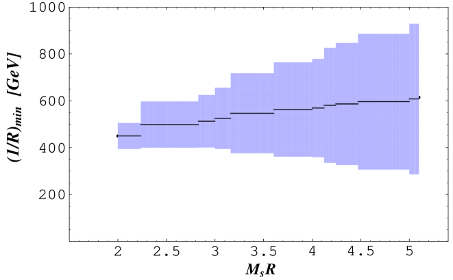
Figure 1: The lower bound on the compactification scale as a function of the cut-off, for $\delta=2$ extra dimensions. The vertical size of the shaded area is given by the loop expansion parameter, $N_{c}\alpha_{3}(M_{s})N_{\rm KK}(M_{s})/(4\pi)$, times the one-loop bound, and is a measure of the theoretical uncertainty. For $M_{s}R\begin{array}[]{c}\,\sim\vspace{-21pt}\\ >\end{array}5$ the standard model interactions become non-perturbative, impeding a reliable estimate of the electroweak observables.

In Fig. 1 we show the dependence of this lower bound on the ratio between the cut-off $M_{s}$ and the compactification scale. Assuming that the theory above $M_{s}$ is custodially symmetric, the one-loop contribution to the $T$ parameter is reliable as long as the theory remains perturbative, roughly for $M_{s}R\begin{array}[]{c}\,\sim\vspace{-21pt}\\ <\end{array}5$. The KK contributions to the one-loop coefficients of the $U(1)_{Y}$, $SU(2)_{W}$ and $SU(3)_{C}$ $\beta$ functions are now $(81/10,\,11/6,\,-2)$, but again the $d$-dimensional $SU(3)_{C}$ interaction becomes non-perturbative in the ultra-violet before the other gauge interactions. The theoretical uncertainty due to higher loops may be estimated in terms of the $\epsilon_{3}$ loop expansion parameter. Fig. 1 shows that the lower bound on $1/R$ is increased by roughly a factor of two compared to the 5-dimensional case, to approximately $400-800$ GeV.

For $d\geq 7$, the cutoff dependence is more severe. The one-loop estimate (3.8) for the $T$ parameter, for example, is enhanced by the factor $(RM_{s})^{d-6}$ relative to the 5-dimensional estimate. Higher loop estimates are of the same order if the ultraviolet cutoff, $M_{s}$, is above the scale where the couplings become nonperturbative. Clearly, no reliable estimate is possible in this case. For smaller $M_{s}$, the one-loop result has a strong dependence on the cutoff, but otherwise the corrections are smaller because the higher-dimensional operators have coefficients suppressed by $1/(M_{s}R)^{\delta}$.

4 Prospects for discovering Kaluza-Klein modes

We have shown that in the case of one universal extra dimension, accessible to all the standard model fields, the fit to the electroweak data allows KK excitations as light as 300 GeV. Such a low bound raises the tantalizing possibility of discovering KK states in the upcoming collider experiments.

If the KK number conservation is exact (that is, there is no additional interaction violating the momentum conservation in extra dimensions,) some of the KK excitations of the standard model particles will be stable. The heavy-generation fermion KK modes can decay to light generation fermion KK modes, e.g., $b^{(1)}\to s^{(1)}(d^{(1)})\,+\,\gamma$, and the $W,Z$ gauge boson KK modes can decay to lepton KK modes and neutrinos, $W^{(1)}(Z^{(1)})\to\ell^{(1)}(\nu^{(1)})\,+\,\nu$. The KK modes of the photon, gluon, and the lightest generation fermions are stable and degenerate in mass, level-by-level, to a very good approximation. Heavy stable charged particles will cause cosmological problems if a significant number of them survive at the time of nucleosynthesis [11]. For example, they will combine with other nuclei to form heavy hydrogen atoms. Searches for such heavy isotopes put strong limits on their abundance. Various cosmological arguments exclude these particles with masses in the range of 100 GeV to 10 TeV, unless there is a low scale inflation that dilutes their abundance [12, 13]. The cosmological problems can be avoided if there exist some KK-number-violating interactions so that the non-zero KK states can decay. The lifetime depends on the strengths of these KK number violating interactions, which are usually suppressed by the cutoff scale and/or the volume factor of the extra dimensions. For collider searches, there is no difference between a stable particle and a long-lived particle which decays outside the detector. We first assume that the KK states are stable or long-lived. The case in which the KK states decay promptly will then be considered when we discuss the possible KK number violating interactions.

4.1 Stable or Long-Lived KK Modes

Because of the KK number conservation, the KK states have to be produced in pairs or higher numbers. They can only be produced at LEP if their masses are less than $E_{\rm CM}/2,\,\sim 100$ GeV. The current lower bound on the size of the extra dimensions is set by the CDF and D0 experiments based on the Run I of the Tevatron. The largest production cross-section is that for KK quarks and gluons. After being produced, they will hadronize into integer-charged states. Because of the large mass, they will be slowly moving and the signatures are highly ionizing tracks.

For one extra dimension of radius $R$, the number of the quark KK modes at each level is twice that of zero-modes, so neglecting the light quark masses, there are six KK quarks of electric charge $-1/3$ and mass $1/R$, four KK quarks of electric charge $2/3$ and mass $1/R$, and two KK top-quarks of mass $\sqrt{1/R^{2}+m_{t}^{2}}$. Therefore, the production cross section for a pair of charged tracks is roughly ten times higher than the one for a $q\bar{q}$ pair of quarks of mass $1/R$, $\sigma_{q\bar{q}}(1/R)$. For $1/R=300$ GeV, $\sigma_{q\bar{q}}(1/R)\approx 0.1$ pb [14].

The current lower mass limits on heavy stable quarks are 195 GeV for charge 1/3 and 220 GeV for charge 2/3 [15]. The reach in mass would be approximately the same for two charge-1/3 quarks as for one charge-2/3 quark. Hence, the current bound on $1/R$ may be approximated as the mass limit on a charge-2/3 quark, but with a production cross section about seven times larger. A dedicated study, beyond the scope of this paper, is required to find this bound precisely. However, by naively extrapolating the mass reach given in [15], we estimate the lower direct bound on $1/R$ to be in the $300-350$ GeV range.

It is remarkable that the direct lower bound on $1/R$ competes with or even exceeds the indirect bound set by the electroweak precision measurements. This should be contrasted with the case of non-universal extra dimensions, where the non-conservation of the KK number makes the indirect bound on $1/R$ stronger than the direct one by a factor of five or so. Thus, Run II at the Tevatron will either discover an universal extra dimension or else it will significantly increase the lower bound on compactification scale.

4.2 Short-Lived KK Modes

As mentioned above, the KK states can decay into ordinary standard model particles if KK number violating effects are present. Such violations of the KK number can occur naturally. For example, the space in which the standard model fields propagate may be a thick brane embedded in a larger space in which gravitons propagate. In this case, the standard model KK excitations can decay into standard model particles plus gravitons going out of the thick brane (or other neutral fields that can propagate outside the thick brane). The unbalanced momentum in extra dimensions can be absorbed by the thick brane. The lifetime depends on the strength of the coupling to the particle going out of the brane and the density of its KK modes (which depends on the volume of the space outside the thick brane). If the KK states produced at the colliders decay promptly inside the detector, the signatures will involve missing energy and will be similar to supersymmetry. We assume that the KK number violating interactions are not large enough to induce a significant single-KK-state production cross section.

For the KK quark and gluon searches, the signature is multi-jets plus missing energy, similar to the squarks and gluinos. At the Tevatron Run I, the lower limits of the squark and gluino mass for the equal mass case are 225 GeV at CDF [16, 17] and 260 GeV at D0 [18, 17]. The production cross-sections of the KK quarks and gluons are similar to those of the squarks and gluinos. The distributions of the jet energies and the missing transverse energy however will depend on the masses of the KK gravitons, i.e., the size of the space outside the thick brane. We expect that the reaches in KK quarks and gluons are comparable to those for squarks and gluinos in supersymmetric models. Run II of the Tevatron is expected to probe squark and gluino masses up to 350–400 GeV [17], so it could also probe KK quarks and gluons beyond the current indirect limit in this scenario. To distinguish the KK states from supersymmetry, however, would require more detailed studies.

Another possibility for KK number violation is that there exist some localized interactions of the standard model fields at a 3+1 dimensional subspace (3-brane) on the boundary or parallel to the boundary. In the effective $d$-dimensional theory, these would take the form of higher dimensional operators suppressed by powers of the cutoff $M_{s}$. Some examples are

$$\int dx^{4}dy\delta(y-y_{0})\frac{\lambda}{M_{s}}\overline{\Psi}\not{\!\!D}\Psi~{},$$

$$\int dx^{4}dy\delta(y-y_{0})\frac{\lambda^{\prime}}{M_{s}^{5/2}}\overline{\Psi}\sigma_{\alpha\beta}F^{\alpha\beta}\Psi~{},$$

$$\int dx^{4}dy\delta(y-y_{0})\frac{\lambda^{\prime\prime}}{M_{s}^{4}}(\overline{\Psi}\Gamma_{A}\Psi)(\overline{\Psi}\Gamma^{A}\Psi),$$ (4.1)

where $\Psi$, $F^{\alpha\beta}$ are five-dimensional standard model fermion and gauge fields, and $\Gamma_{A}$ is some combination of the $\gamma$ matrices. The first contributes to the kinetic terms of the KK states, so the KK mass spectrum would be modified after re-diagonalizing and rescaling the kinetic terms into the canonical form [19]. The corrections (4.1) are suppressed by $M_{s}$ and we assume that the coefficients ($\lambda,\,\lambda^{\prime},\,\lambda^{\prime\prime},...$) are small enough so that these operators do not affect our analysis of electroweak observables. However, they could be sufficiently large to allow decays within the detector of the pair-produced KK modes. The decay channels depend on which KK number violating interactions are present. We discuss the simplest two-body decays which can be induced by, e.g., the first two interactions in eq. (4.2).

If the interactions involving the gluon field dominate, the KK quarks and gluons decay into jets. The signals would be multi-jets which are difficult to extract from the QCD backgrounds at the Tevatron. However, if the interactions involving the electroweak gauge bosons are large enough so that the decay of the KK quarks into electroweak gauge bosons and quark zero-modes has a significant branching ratio, we can invoke the searches for the heavy quarks. For the decay into the $W$ bosons, the signal is similar to the top quark. One can use the measurements of the top quark production cross section at the Tevatron [20, 21] to put limits on the new heavy quarks. In Ref. [22], Popovic and Simmons derived the bounds $\sigma^{q_{H}}(B_{W})^{2}<7.8\,{\rm pb}\,(12.0\,{\rm pb})$ at D0 (CDF), where $\sigma^{q_{H}}$ is the cross-section for the heavy quark production, and $B_{W}$ is the branching ratio for the heavy quark decaying to the $W$ boson and an ordinary quark. Applying this result, we have $1/R\begin{array}[]{c}\,\sim\vspace{-21pt}\\ >\end{array}200$ GeV for $B_{W}\sim 50\%$. There is also a search for the fourth generation $b^{\prime}$ quark through the decay mode $ZZb\bar{b}$ at CDF, which excluded the $b^{\prime}$ quark mass between 100 and 199 GeV if the branching ratio is 100% [23]. This can also apply to the KK states of the $b$ quark. In Run II at the Tevatron, the decays of quark KK modes into a quark zero-mode and a photon may be also significant. Other processes, potentially relevant for Run II, include the electroweak production of a pair of lepton KK modes with each of them subsequently decaying into a lepton zero-mode and a photon or a $W^{\pm}$, and the production of a pair of KK modes of the electroweak gauge bosons leading to a four-lepton signal. In general, the direct bounds on $1/R$ are weaker and model dependent in this case.

With more extra dimensions the production cross section is higher because of the multiplicity of KK modes. For example, with two extra dimensions there are twice as many KK modes of mass $1/R$ than in the case of one extra dimension. However, the indirect bounds may also be significantly higher. It is not clear whether they are within the reach of Run II. The sensitivity of the LHC, though, should be impressive, above a few TeV.

5 Summary

We have examined the experimental consequences of higher dimensional theories in which all the standard model fields propagate in the extra dimensions. With these “universal” extra dimensions, contributions to precision electroweak observables arise first at the one-loop level. In the case of a single extra dimension, where the one-loop computations can be done reliably within the framework of the effective 5-dimensional standard model, the electroweak observables were estimated to allow a compactification scale as low as $300$ GeV. We then noted that the current lower bound from direct production experiments is set by CDF and D0 to be in the few-hundred GeV range. Thus Run II at the Tevatron will either see evidence for the extra dimensions or significantly raise the lower bound on the compactification scale.

In the case of two universal extra dimensions, the electroweak observables become logarithmically sensitive, at one loop, to the cutoff on the effective 6-dimensional theory. If the cutoff is taken to be as large as possible, where this effective theory becomes strongly coupled, then the theory cannot be used to compute reliably the electroweak observables. If, on the other hand, the cutoff is lower, with no important contributions to the electroweak observables from higher scales, then the observables may be estimated reliably at the one-loop level. As indicated in Fig. 1, with $M_{s}R\leq 5$, the lower bound on the compactification scale is estimated to be between $400$ GeV and $800$ GeV.

Besides opening the possibility of experimental detection of universal extra dimensions in the near future, the lower bound on the compactification scale discussed here suggests that physics in extra dimensions may be responsible for electroweak symmetry breaking. For example, standard model gauge interactions may produce a bound-state Higgs doublet in six dimensions [4] without excessive fine-tuning.

Acknowledgements:  We would like to thank Mike Albrow, Zacharia Chacko, Lance Dixon, Jonathan Feng, Sheldon Glashow, Kevin Lynch, Eduardo Ponton, Marko Popovic, Erich Poppitz, Martin Schmaltz, Elizabeth Simmons, Matt Strassler, and Neal Weiner for helpful conversations and comments. The work of T. Appelquist and B. A. Dobrescu was supported by DOE under contract DE-FG02-92ER-40704. H.-C. Cheng is supported by the Robert R. McCormick Fellowship and by DOE Grant DE-FG02-90ER-40560.

References

- [1] K.R. Dienes, E. Dudas and T. Gherghetta, “Extra spacetime dimensions and unification,” Phys. Lett. B436, 55 (1998) hep-ph/9803466.
- [2] I. Antoniadis, “A Possible New Dimension At A Few TeV,” Phys. Lett. B246, 377 (1990).
- [3] N. Arkani-Hamed and M. Schmaltz, “Hierarchies without symmetries from extra dimensions,” Phys. Rev. D61, 033005 (2000) hep-ph/9903417.
- [4] N. Arkani-Hamed, H.-C. Cheng, B. A. Dobrescu and L. J. Hall, “Self-breaking of the standard model gauge symmetry,” Phys. Rev. D62, 096006 (2000) hep-ph/0006238.
-
[5]
W. J. Marciano, “Precision electroweak
measurements and ’new physics’,” hep-ph/9902332 and “Fermi
constants and ’new physics’,” Phys. Rev. D60, 093006
(1999), hep-ph/9903451;
P. Nath and M. Yamaguchi, “Effects of extra space-time dimensions on the Fermi constant,” Phys. Rev. D60, 116004 (1999), hep-ph/9902323;
M. Masip and A. Pomarol, “Effects of SM Kaluza-Klein excitations on electroweak observables,” Phys. Rev. D60, 096005 (1999), hep-ph/9902467;
T. G. Rizzo and J. D. Wells, “Electroweak precision measurements and collider probes of the standard model with large extra dimensions,” Phys. Rev. D61, 016007 (2000), hep-ph/9906234;
A. Strumia, “Bounds on Kaluza-Klein excitations of the SM vector bosons from electroweak tests,” Phys. Lett. B466, 107 (1999), hep-ph/9906266;
R. Casalbuoni, S. De Curtis, D. Dominici and R. Gatto, “SM Kaluza-Klein excitations and electroweak precision tests,” Phys. Lett. B462, 48 (1999), hep-ph/9907355;
C. D. Carone, “Electroweak constraints on extended models with extra dimensions,” Phys. Rev. D61, 015008 (2000), hep-ph/9907362;
A. Delgado, A. Pomarol and M. Quiros, “Electroweak and flavor physics in extensions of the standard model with large extra dimensions,” JHEP 0001, 030 (2000), hep-ph/9911252. - [6] M. B. Green and J. H. Schwarz, “Anomaly Cancellation In Supersymmetric D=10 Gauge Theory And Superstring Theory,” Phys. Lett. B149, 117 (1984).
- [7] H.-C. Cheng, B. A. Dobrescu and C. T. Hill, “Gauge coupling unification with extra dimensions and gravitational scale effects,” Nucl. Phys. B573, 597 (2000), hep-ph/9906327.
- [8] T. Appelquist and G. Wu, “The Electroweak chiral Lagrangian and new precision measurements,” Phys. Rev. D48, 3235 (1993), hep-ph/9304240.
- [9] R. S. Chivukula, C. Holbling and N. Evans, “Limits on a composite Higgs boson,” Phys. Rev. Lett. 85, 511 (2000), hep-ph/0002022.
-
[10]
The LEP Electroweak Working Group,
http://lepewwg.web.cern.ch/LEPEWWG/plots/summer2000/ -
[11]
A. De Rujula, S. L. Glashow and
U. Sarid, “Charged Dark Matter,” Nucl. Phys. B333, 173
(1990);
S. Dimopoulos, D. Eichler, R. Esmailzadeh and G. D. Starkman, “Getting A Charge Out Of Dark Matter,” Phys. Rev. D41, 2388 (1990);
R. S. Chivukula, A. G. Cohen, S. Dimopoulos and T. P. Walker, “Bounds On Halo Particle Interactions From Interstellar Calorimetry,” Phys. Rev. Lett. 65, 957 (1990);
A. Gould, B. T. Draine, R. W. Romani and S. Nussinov, “Neutron Stars: Graveyard Of Charged Dark Matter,” Phys. Lett. B238, 337 (1990). - [12] L. Randall and S. Thomas, “Solving the cosmological moduli problem with weak scale inflation,” Nucl. Phys. B449, 229 (1995), hep-ph/9407248.
- [13] D. H. Lyth and E. D. Stewart, “Thermal inflation and the moduli problem,” Phys. Rev. D53, 1784 (1996), hep-ph/9510204.
- [14] R. K. Ellis, “Rates for top quark production,” Phys. Lett. B259, 492 (1991).
- [15] A. Connolly [CDF collaboration], “Search for long-lived charged massive particles at CDF,” Talk at the American Physical Society (APS) Meeting of the Division of Particles and Fields (DPF 99), Los Angeles, CA, Jan 5-9, 1999, hep-ex/9904010.
- [16] J. P. Done [CDF collaboration], Talk at the American Physical Society Centennial Meeting, Atlanta, GA, March 20–26, 1999.
- [17] S. Abel et al. [SUGRA Working Group Collaboration], “Report of the SUGRA working group for run II of the Tevatron,” hep-ph/0003154.
- [18] B. Abbott et al. [D0 Collaboration], “Search for squarks and gluinos in events containing jets and a large imbalance in transverse energy,” Phys. Rev. Lett. 83, 4937 (1999), hep-ex/9902013.
- [19] R. Barbieri, L. J. Hall and Y. Nomura, “A Constrained Standard Model from a Compact Extra Dimension,” hep-ph/0011311.
- [20] S. Abachi et al. [D0 Collaboration], “Measurement of the top quark pair production cross section in p anti-p collisions,” Phys. Rev. Lett. 79, 1203 (1997), hep-ex/9704015.
- [21] F. Abe et al. [CDF Collaboration], “Measurement of the top quark mass and t anti-t production cross section from dilepton events at the Collider Detector at Fermilab,” Phys. Rev. Lett. 80, 2779 (1998), hep-ex/9802017.
- [22] M. B. Popovic and E. H. Simmons, “Weak-singlet fermions: Models and constraints,” Phys. Rev. D62, 035002 (2000), hep-ph/0001302.
- [23] T. Affolder et al. [CDF Collaboration], “Search for a fourth-generation quark more massive than the Z0 boson in p anti-p collisions at = 1.8 TeV,” Phys. Rev. Lett. 84, 835 (2000), hep-ex/9909027.