Polarized Proton Nucleus Scattering

Abstract

We show that, to a very good approximation, the ratio of the spin-flip to the non-flip parts of the elastic proton-nucleus amplitude is the same as for proton-nucleon scattering at very high energy. The result is used to do a realistic calculation of the analyzing power $A_{N}$ for $pC$ scattering in the Coulomb-nuclear interference (CNI) region of momentum transfer.

1. Nuclear modification of the spin amplitudes: optical model for large nuclei

It is important, especially for the purposes of polarimetry, to have an estimate of the small momentum transfer spin-flip $pA$ scattering in terms of that for $pp$ elastic scattering [1]. That is the purpose of this paper. We focus on the analyzing power for the proton $A_{N}$, which is the asymmetry between scattering of the proton polarized up versus down with regard to the scattering plane. Since this is known to be small, as are the other spin-dependent amplitudes for $pp$ elastic scattering, if we work to lowest order in this amplitude we can disregard the spin of the nucleons within the nucleus.

We are left with only two spin amplitudes in $pp$ elastic scattering

$$f(q)=f_{o}(q)+\vec{\sigma}\,\cdot\frac{\vec{k}\times\vec{k}^{\prime}}{|\vec{k}\times\vec{k}^{\prime}|}\ f_{s}(q)\ ,$$ (1)

where $\vec{k}$ and $\vec{k}^{\prime}$ are the initial and final nucleon momenta in c.m., $\vec{\sigma}$ are the Pauli matrices, $f_{o}(q)$ and $f_{s}(q)$ are the non-flip and spin-flip amplitudes. These correspond, up to a constant normalization factor, to the $pp$ amplitudes $\phi_{+}=(\phi_{1}+\phi_{3})/2$ and $\phi_{5}$, respectively [2]. $\vec{q}=\vec{k}-\vec{k}^{\prime}$ is the vector of momentum transfer; it is normal to $\vec{k}$ for small angle scattering. The normalization of the amplitudes is fixed by the relation,

$$2\ f_{o}(0)=i\sigma^{NN}_{tot}(1-i\rho)\ ,$$ (2)

where $\sigma_{\rm tot}$ is the $pp$ total cross section, which is taken to be the same as the $pn$ cross section at high energy, and $\rho$ is the forward ratio of real to imaginary parts of the elastic amplitudes.

We transform these to impact parameter $b$-space via

$$f(q)=\int d^{2}b\,e^{i\vec{q}\cdot\vec{b}}\,(\tilde{f}_{o}(b)+i\,\vec{\sigma}\cdot(\hat{b}\times\hat{k})\,\tilde{f}_{s}(b)).$$ (3)

Correspondingly, we denote the elastic proton-nucleus amplitudes by $F_{o}(q)$ and $F_{s}(q)$; they are related by Fourier transform to the partial amplitude $\tilde{F}_{o,s}(b)$ in impact-parameter representation, just as in Eq. (3).

In the eikonal approximation [3] the proton-nucleus amplitude is expressed through the eikonal $\chi(\vec{b})$ by

$$\tilde{F}(b)=i\,(1-e^{\chi(b)})\ ,$$ (4)

where for large nuclei

$$\chi(\vec{b})=i\,\int d^{2}s\,\left[\tilde{f}_{o}(s)+i\,\vec{\sigma}\cdot(\hat{s}\times\hat{k})\,\tilde{f}_{s}(s)\right]\ T(\vec{b}-\vec{s})\ .$$ (5)

Here $\hat{k}$ and $\hat{s}$ are the unit vectors directed along $\vec{k}$ and $\vec{s}$ respectively. $T(b)$ is the nuclear thickness function,

$$T_{A}(b)=\int\limits_{-\infty}^{\infty}dz\,\rho_{A}(b,z)\ ,$$ (6)

and $\rho_{A}(b,z)$ is the nuclear density which depends on $b$ and and the longitudinal coordinate $z$.

If the radius of the nucleus substantially exceeds the radius of interaction, the latter can be neglected calculating the non-flip eikonal,

$$\chi_{o}(b)\approx i\,T_{A}(b)\,\int d^{2}s\,\tilde{f}_{o}(s)=i\,T_{A}(b)f_{o}(0)\ ,$$ (7)

which is the usual approximation. For the spin-flip eikonal, however, such an approximation leads to zero result. Indeed, the “spin-orbit coupling” $\vec{\sigma}\cdot(\vec{s}\times\vec{k})$ leads to cancelation on integration over $\vec{s}$. The lowest order nonvanishing approximation is

$$T_{A}(\vec{b}-\vec{s})\approx T_{A}(b)-\vec{s}\cdot\vec{\nabla}_{b}\,T_{A}(b).$$ (8)

The corresponding eikonal is

$$\chi_{s}(b) = -\frac{1}{2}\,\sigma\cdot(\hat{k}\times\nabla_{b})T_{A}(b)\int d^{2}s\,s\,\tilde{f}_{s}(s)$$

$$= \sigma\cdot(\hat{k}\times\nabla_{b})T(b)\left.\frac{df_{s}(q)}{dq}\right|_{q=0}\,.$$

The spin-flip amplitude vanishes as $\sqrt{-t}$ in the forward direction, and so it can be represented as

$$f_{s}(q)=\mu_{P}(q)\,\frac{q}{2m_{N}}\,f_{o}(q)\ ,$$ (10)

where, for the strong interaction part of the amplitude, $\mu_{P}(q)$ is a complex function which is regular as $t\to 0$. Therefore

$$\chi(b)=\left[1+\frac{i\,\mu_{P}(0)}{2m_{N}}\,\vec{\sigma}\cdot(\hat{k}\times\nabla_{b})\right]\,i\,f_{o}(0)\,T_{A}(b)\ .$$ (11)

From this, the amplitude for polarized proton - nucleus elastic scattering in optical approximation and the first order in $\mu_{P}$ reads,

$$F_{o}(q)=i\,\int d^{2}b\,e^{i\,\vec{q}\cdot\vec{b}}\,\left(1-e^{i\,f_{o}(0)\,T_{A}(b)}\right)$$ (12)

$$F_{s}(q)=\,\frac{\mu_{P}(0)\,f_{o}(0)}{m_{N}}\,\int d^{2}b\,e^{i\,\vec{q}\cdot\vec{b}}\,(\hat{q}\cdot\nabla_{b})T_{A}(b)\,e^{i\,f_{o}(0)\,T_{A}(b)}$$ (13)

Integrating this expression by parts we arrived at a surprising result,

$$F_{s}(q) = i\,\mu_{P}(0)\,\frac{q}{2m_{N}}\,\int d^{2}b\,e^{i\,\vec{q}\cdot\vec{b}}\,\left(1-e^{if_{o}(0)T_{A}(b)}\right)$$ (14)

$$= \mu_{P}(0)\,\frac{q}{2m_{N}}\,F_{o}(q)\ :$$

both the non-flip and the spin-flip parts of the elastic amplitude have the same nuclear form factor $F_{o}(q)\,$!

This is not a trivial conclusion since the homogeneous central nuclear region does not contribute to the spin-flip amplitude, which according to Eq.(8) is proportional to the derivative of nuclear thickness, i.e. gains its value only from the nuclear periphery. On the contrary, the non-flip part of the amplitude is large at $b<R_{A}$ and small at the nuclear edge. This is compensated for partially by the fact that the derivative near the nuclear surface is large, proportional to the nuclear radius $R_{A}$, and partially due to the variation of the phase factor around the periphery which yields on integration a factor $iqR_{A}$. Therefore, $F_{s}$ has the same $A$ dependence as $F_{o}$, i.e. $A^{2/3}$. Furthermore, their relative phase is independent of $q$.

This result requires that the nuclear size be much larger than the slopes for $pp$ scattering; i.e. $R_{A}^{2}\gg 2B_{o}$ and $R_{A}^{2}\gg 2B_{s}$. Since $2B_{o}$ is about $20\,GeV^{-2}$ and $R_{A}^{2}$ ranges from about $50\,GeV^{-2}$ to $500\,GeV^{-2}$ from $He$ to $Pb$ [4], this strong inequality is not satisfied over much of the periodic table and corrections need to be taken into account.

2. Finite size corrections and a little theorem

The presentation in previous section was maximally simplified for the sake of clarity. Some corrections need to be discussed. In the case of smaller nuclei, one should use more accurate approximations. Again, following Glauber [3], for a nucleus of $A$ nucleons with wave function in coordinate space $u(x_{1},\dots x_{A})$ the amplitude for $pA$ elastic scattering is given by

$$F(q)=i\int d^{2}b\,e^{i\vec{q}\cdot\vec{b}}\left\{\int d^{3}x_{1}\dots d^{3}x_{A}|u(x_{1},\dots x_{A})|^{2}\left[1-\prod_{j}(1+i\tilde{f}(\vec{b}-\vec{s}_{j})\right]\right\}$$ (15)

where $s_{j}$ is the transverse component of $x_{j}$. We assume that the $pp$ and $pn$ amplitudes are the same at the energy of interest and continue to neglect the spin of the nucleons within the nucleus.

For a specific nucleus with known wave-function one could do this numerically with an assumed form for the scattering amplitudes $f$. We will do this for an interesting case shortly. Before doing so we will prove a theorem which yields a very general result for a special case. Let us assume that Eq. (10) is valid with $\mu_{P}$ independent of $q$. This is true in some models and likely not to be too far wrong. Then it is easy to show that

$$\tilde{f}_{s}(b)=\frac{\mu_{P}}{2m_{N}}\frac{d\tilde{f}_{o}(b)}{db}.$$ (16)

Then we have

$$\frac{\mu_{P}}{2m_{N}}\frac{\partial}{\partial b}\,\left[1-\prod_{j}(1+i\tilde{f}(\vec{b}-\vec{s}_{j})\right] = -i\,\frac{\mu_{P}}{2m_{N}}\sum_{i}\frac{\partial\tilde{f}_{i}(\vec{b}-\vec{s}_{i})}{\partial b}\prod_{j\neq i}\Bigl{[}1+i\,\tilde{f}(\vec{b}-\vec{s}_{j})\Bigr{]}$$ (17)

$$= -i\,\sum_{i}(\hat{b}\cdot\widehat{b-s_{i}})\tilde{f}_{s}(b-s_{i})\prod_{j\neq i}\Bigl{[}1+i\,\tilde{f}(b-s_{j})\Bigr{]}.$$

Now expand Eq. (15) keeping linear terms in $f_{s}$, take the trace with $\vec{\sigma}\cdot\hat{b}\times\hat{k}/2$ of the factor in brackets; this operation will produce the argument of the integral for $i\tilde{F}_{s}(b)$. This is easily seen to match the structure given in Eq.(17). Thus

$$\tilde{F}_{s}(b)=\frac{\mu_{P}}{2m_{N}}\frac{d\tilde{F}_{o}(b)}{db},$$ (18)

and by the inverse of the process used to obtain Eq.(17) we obtain as a theorem, with very weak assumptions on the nuclear structure,

$$F_{s}(q)=\frac{\mu_{P}}{2m_{N}}F_{o}(q).$$ (19)

The result obtained in Section 1 may be seen as a special case of this since for $R_{A}^{2}\gg 2B_{o}$ and $R_{A}^{2}\gg 2B_{s}$ the two amplitudes have effectively the same shape in $q$ over the relevant range.

Long ago Bethe [5] carried out calculations with similar goals to ours for low-energy, potential scattering. He cites there the analogous result to Eq. (14) as obtained by Köhler and by Levintov [6], demonstrating how widely applicable this relation is. See also [7].

We test the robustness of this result by evaluating Eq. (18) numerically for $H\!e^{4}$, dropping the assumptions that the slopes of the non-flip and flip amplitudes are the same and that the nucleus is large. We adopt the independent particle wave function

$$u(x_{1},x_{2},x_{3},x_{4})=\prod_{i}u(x_{i})$$ (20)

with

$$u(x)=Ne^{-\frac{x^{2}}{2R_{A}^{2}}}$$ (21)

for each of the 4 nucleons in the nucleus. We follow the method used by Bassel and Wilkin [8] many years ago for calculating the non-flip amplitude. Their results agree rather well with data at low energy up to about the first diffraction dip so it should be a useful indicator of the robustness of this result. As before we calculate to first order in $f_{s}$. We use the exponential forms for the scattering amplitude near $t=0$, neglecting the real parts; this should be sufficiently accurate for the small-$t$ predictions:

$$2f_{o}(q) = i\,\sigma_{\rm tot}e^{-\frac{q^{2}R_{o}^{2}}{4}}$$ (22)

$$2f_{s}(q) = i\,\frac{\mu_{P}}{2m_{N}}\,\sigma_{\rm tot}\,e^{-\frac{q^{2}R_{s}^{2}}{4}}.$$

Define $F_{s}^{\rm red}$ by $F_{s}(q)=q\,\mu_{P}/2\,m_{N}\,F_{s}^{\rm red}(q)$. We will use the parameters $R_{A}^{2}=50\,GeV^{-2}$ [4], $R_{o}^{2}=24\,GeV^{-2}$ [1] and will vary $R_{s}$ from small values up to $1.4\,R_{o}$. In Fig.1 the results of this calculation are displayed by plotting $F_{s}^{\rm red}(0)/F_{o}(0)$ as a function of $R_{s}/R_{o}$.

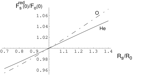
Figure 1: The ratio of the reduced nuclear spin-flip amplitude to the non-flip amplitude at $t=0$ as a function of the ratio of the square-root of the slopes $R_{s}/R_{o}$ for $H\!e^{4}$ and $O^{16}$.

We see that it goes through 1 at $R_{s}=R_{o}$ as required by our theorem and that it varies by less than about $\pm 5\%$ over this rather large range of variation for the slopes. Thus, within the approximations of standard multiple scattering theory we can be confident that the ratio of flip to non-flip for $pA$ scattering will be reasonably close to that for $pp$ scattering.

We have carried through the same calculation for $O^{16}$ using again the wave-functions of [8]. The results are also shown in Fig.1. The sensitivity to $R_{s}/R_{0}$ is slightly greater than for $H\!e^{4}$, but still not very large. In order to estimate how this goes as the nuclei grow we have modeled the problem with all Gaussian wave functions with radius growing as $A^{1/3}$ and taken the derivative with respect to $R_{s}/R_{0}$ of the amplitude at $t=0$ and $R_{s}/R_{0}=1$. This is shown as a function of $A$ over a very wide range in Fig.2. We see that the maximum correction occurs near oxygen, but the effect falls off very slowly with $A$ and is still a few percent at lead.

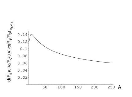
Figure 2: The derivative of the ratio of the reduced nuclear spin-flip amplitude to the non-flip amplitude at $t=0$ and $R_{s}/R_{0}=1$ as a function of the nuclear number A.

3. Inelastic shadowing

A potentially serious correction to these calculations, especially at higher energy, is inelastic shadowing. In the Glauber-type calculations only multiple elastic scattering is taken into account, whereas diffractive production of excited states which rescatter back into the proton state should also be taken into account. This was emphasized by Gribov long ago [9]. Furthermore, there is experimental evidence in the non-flip scattering that inelastic shadowing is important at high energy [10]. One does not have the knowledge of inelastic spin-flip scattering in the hadronic basis in order to do a direct phenomenological calculation of this correction.

An effective way to think about these corrections in all orders is to switch to the basis of interaction eigenstates in which the amplitude matrix is diagonal [11]. In QCD such a basis is given by the color-dipole light-cone representation [12] widely used nowadays. Thus, Eq.(5) should be replaced by

$$\tilde{F}(b)=i\,\left\langle 1-e^{\chi(b)}\right\rangle\ ,$$ (23)

where the eigenvalue of the amplitude is averaged over all eigenstates (in QCD they are the Fock components with definite transverse separations). On the contrary, in the Glauber approximation only the exponent in Eq.(5) would be averaged ($\chi\Rightarrow\langle\chi\rangle$). The difference between these two ways of averaging is just the Gribov’s inelastic correction [11, 12].

The eigenstate representation for inelastic corrections is rather simple and allows to sum up all of them in all orders. However, it needs quite high energies to prevent the eigenstates from mixing (in the dipole picture the parton separations should be frozen for the time of propagation through the nucleus). At medium high energies this condition is not met and the amount of inelastic shadowing shrinks. This is controlled by the longitudinal nuclear form factor [13],

$$F^{2}_{A}(q_{\scriptscriptstyle L})=\frac{1}{A\,\langle T_{A}\rangle}\int d^{2}b\,\left|\int\limits_{-\infty}^{\infty}dz\,\rho_{A}(b,z)\,e^{{\displaystyle i\,q_{\scriptscriptstyle L}z}}\right|^{2}\ ,$$ (24)

where

$$\langle T_{A}\rangle={1\over A}\int d^{2}b\,T_{A}^{2}(b)$$ (25)

is the mean nuclear thickness; $q_{L}=(M^{2}-m_{N}^{2})/2E_{p}$, $E_{p}$ is the proton lab frame energy and $M$ is the the mass of the diffractively excited proton, which one should integrate over. Calculations and data [10] show that the inelastic corrections are quite small at the AGS energies and the Glauber approximation works pretty well.

On the contrary, at the high energies of RHIC one can rely on the opposite limit of frozen eigenstates (23), or $F^{2}_{A}(q_{L})=1$. Correspondingly, this modification of the amplitude should be applied to the non-flip spin amplitude Eq. (12) and to the spin-flip amplitude Eq. (13) and the upper line of (14). The result for the spin-flip amplitude is not obvious since $\mu_{P}$ may correlate to eigenstates and should be involved into the averaging.

For the lowest Fock component of the proton, $|3q\rangle$, we expect that averaging of $\mu_{P}$ weighted with the wave function squared decouples from averaging of the exponential in the upper row of Eq. (14). This is certainly true if the spin-flip part originates solely from the anomalous color magnetic moment of the quark [14]. However, it can also be a result of the Melosh spin rotation effect. Although helicity is invariant relative to a longitudinal Lorentz boost, the proton and the quark helicities are defined relative to different axes because of the transverse motion of the quarks. It turns out, however, that the spin rotation corrections cancel if the radial part of the proton wave function is symmetric. Only if the proton wave function is dominated by configurations with a small diquark does the proton-Pomeron vertex acquire a spin-flip part $\mu_{P}$ [15]. It is sensitive to the smallest size in the proton (diquark), while $f_{0}(0)$ in the exponent in Eq.(14) is sensitive to the largest inter-quark spacing in the proton. Therefore, integrations over these two distances factorize and the relation Eq.(14) is preserved.

One can also look at this problem from the point of view of the triple-Regge phenomenology and evaluate the corrections. The Fock state $|3q\rangle$ of the proton and the higher components $|3q\,nG\rangle$ in which the slowest parton is a valence quark correspond to the triple Regge graph PPR shown in Fig. 3.

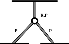
Figure 3: The triple-Regge graph, where a unitarity cut of the upper leg corresponds to the $|3q\rangle$ (PPR) or $|3q\,nG\rangle$ (PPP) Fock components.

The leading Reggeons $R=\omega,\ f$ are known to have a small spin-flip amplitude, and there is a danger that they may affect the eikonal relation Eq.(14) via corresponding inelastic corrections.

On expanding the exponential in Eq. (23) one finds the relative inelastic correction in the lowest order for the non-flip amplitude [13],

$$-\,\frac{\Delta\tilde{F}(b)}{\tilde{F}(b)}={1\over 4}\,\langle T_{A}\rangle\,\left(\frac{d\sigma_{sd}/dt}{d\sigma_{el}/dt}\right)_{t=0}\ ,$$ (26)

where $\langle T_{A}\rangle$ is the mean nuclear thickness function defined in Eq.(25).

The forward single diffractive $pp\to pX$ cross section corresponding to the $PPR$ contribution integrated over effective mass of the produced system $X$ reads, [16]

$$\left.\frac{d\sigma^{PPR}_{sd}}{dt}\right|_{t=0}=2\,G_{PPR}(0)\,\sqrt{\frac{s_{0}}{M_{0}^{2}}}\ ,$$ (27)

where the triple-Regge coupling $G_{PPR}(0)=2-3\,{\rm mb/GeV}^{2}$ was fitted to data in [16]; $s_{0}=1\,GeV^{2}$; $M_{0}\sim 1\,GeV$ is the bottom limit for integration over masses.

Thus, the energy independent fraction of low-mass diffractive excitation of (the PPR term) relative to the elastic cross section is,

$$\left(\frac{d\sigma^{PPR}_{sd}/dt}{d\sigma_{el}/dt}\right)_{t=0}\approx 0.06\ .$$ (28)

The corresponding inelastic correction Eq.(26) grows $\propto A^{1/3}$ and ranges from about $1\%$ for carbon to about $2\%$ for lead. These values demonstrate that a possible deviation from relation Eq.(14) caused by inelastic correction related to the $PPR$ triple-Reggeon term, or the $|3q\rangle$ Fock component of the proton, is expected to be very small. This estimate also confirms that the approximation of lowest order in multiple scattering expansion in Eq.(26) is rather accurate for all nuclei.

The higher order Fock components $|3q\,nG\rangle$ in which the parton carrying the least fraction of the light-cone momentum is a gluon, correspond to triple-Pomeron term $PPP$. We do not expect any substantial deviation from relation Eq.(14) due to the related inelastic corrections either. Indeed, radiation of a gluon with small fraction $x\ll 1$ of the light-cone momentum does not flip the quark helicity [17], the same as the $t$-channel gluons in the Pomeron. One can reformulate this statement in terms of the standard Regge phenomenology.

One way of doing this is to use the fan diagrams introduced by Schwimmer [18], and further developed recently by Bondarenko et al. [19]. The approximations used are best justified for large nuclei, and it is not clear at present how accurate the results are quantitatively. Nevertheless, we apply it to the problem at hand. The typical fan diagram is shown in Fig.4.

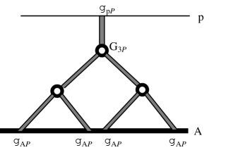
Figure 4:

Typical Pomeron fan diagram. $g_{AP}(b)=A\frac{g_{{\rm p}P}}{\pi R_{A}^{2}s_{0}}\exp(-b^{2}/R_{A}^{2})$

The crucial feature is that the incident proton couples to a single Pomeron, which is taken to be a pole a small amount $\Delta$ above 1. This then branches into a fan of Pomerons, via the triple Pomeron coupling $G_{3P}$, which then couple to the nucleus. In order to sum these graphs, the $q^{2}$-dependence of the propagators and the various vertices (except the coupling to the nucleus) is neglected with regard to the rapid $q^{2}$ dependence coming from the nucleon form factor. The sum of these graphs in the form given by [19] is

$$\tilde{F}^{\rm fan}_{o}(b)=i(s/s_{0})^{\Delta}\,(A/2\pi R_{A}^{2})\,\frac{g_{pP}^{2}}{1+\kappa_{A}(b)}e^{-b^{2}/R_{A}^{2}},$$ (29)

where

$$\kappa_{A}(b)=g_{AP}(b)\,G_{3P}\,\frac{(s/s_{0})^{\Delta}-1}{\Delta}.$$ (30)

$g_{{\rm p}P}$ denotes the Pomeron non-flip coupling to the proton which is constant in this approximation. By factorization of the Pomeron coupling, the spin-flip coupling is $g_{s}(q)=\mu_{P}\,(q/{2m_{N}})g_{{\rm p}P}$. Therefore to this approximation the relation $F_{s}(q)=\mu_{P}\,(q/{2m_{N}})\,F_{o}(q)$ is trivially maintained. Correspondingly,

$$\tilde{F}_{s}^{\rm fan}(b)=(\mu_{P}/{2m_{N}})\,\frac{d\tilde{F}_{o}^{\rm fan}(b)}{db}.$$ (31)

It may be that this approximation is improved by eikonalizing it in the usual way [18, 19]:

$$\tilde{F}^{\rm fan}\to-i\,\chi(b).$$ (32)

This improved approximation, call it $\tilde{F}^{\rm eik}(q)$ then clearly satisfies

$$\tilde{F}_{s}^{\rm eik}(b) = (\mu_{P}/2m_{N})\,\frac{d\tilde{F}_{o}^{\rm fan}(b)}{db}e^{i\,\tilde{F}_{o}^{\rm fan}(b)}$$

$$= i\,(\mu_{P}/2m_{N})\,\frac{d(1-e^{i\,\tilde{F}_{o}^{\rm fan}(b)})}{db}$$

$$= \frac{d\tilde{F}_{o}^{\rm eik}(b)}{db},$$

and so the relation is preserved in this approximation as well [7]. Only the inelastic corrections related to small mass excitation, or $PPR$ triple-Regge term, cannot be included in eikonalization, but they are found above to be small.

It is clear from these estimates that the relation Eq. (18) is very robust; however, we know from Section 2 that it cannot be exact. The inelastic corrections important at high energies are more poorly under control and it would be desirable to eventually have better estimates of these.

4. Polarized proton-nucleus scattering and the spin-flip Pomeron amplitude

In this section we will use the results of the preceding sections, in particular Eq(14), to calculate the analyzing power $A_{N}$ for $pA$ scattering in the small $t$ region, $|t|\leq 0.1{\rm GeV}/c^{2}$. Since $\mu_{P}$ is not disturbed by nuclear effects, one can use elastic $pA$ scattering to determine this parameter. Although many experimental and theoretical results restrict $\mu_{P}$ to be less than about $0.1-0.2$ [1](see also [20]), none of them is strong enough or sufficiently reliable. A promising way to fix $\mu_{P}$ from data is to measure the analyzing power $A_{N}$ of scattering of protons with known polarization off protons [15, 21] or nuclei [22] in the Coulomb-nucleus interference region of $q^{2}$ [23]. Hunting for the spin-flip part of the Pomeron amplitude it is important to disentangle it from the contribution of secondary Reggeons which is still quite important at medium high energies. This is an important advantage of nuclear targets which either completely eliminate the main source of the spin-flip amplitude if the nucleus is isoscalar, the isovector Reggeons $\rho$ and $a_{2}$, or suppress them by $1/A$.

The $t$ - dependence of $A_{N}$ in polarized elastic $p-A$ scattering in the CNI region is similar to that in $pp$ scattering. In particular, they both have a distinctive peak in the neighborhood of $t=-.002{\rm GeV}/c^{2}$. However, the spin asymmetry as function of $t=-q^{2}$ is substantially modified by nuclear effects [22] compared to $pp$ scattering over the range we are interested in here [23, 2, 1]. In the notation of [1],

$$\frac{16\,\pi}{(\sigma^{pA}_{tot})^{2}}\,\frac{d\,\sigma_{pA}}{d\,t}\,A^{pA}_{N}(t)=\frac{\sqrt{-t}}{m_{N}}\,F_{A}^{h}(t)\,\biggl{\{}F_{A}^{em}(t)\,\frac{t_{c}}{t}\,\Bigl{[}(\mu_{p}-1)(1-\delta_{pA}\,\rho_{pA})$$ (34)

$$- 2\,({\rm Im}\,r^{pA}_{5}-\delta_{pA}\,{\rm Re}\,r^{pA}_{5})\Bigr{]}-2\,F_{A}^{h}(t)\Bigl{(}{\rm Re}\,r^{pA}_{5}-\rho_{pA}\,{\rm Im}\,r^{pA}_{5}\Bigr{)}\biggr{\}}\ ,$$

where

$$\frac{16\,\pi}{(\sigma^{pA}_{tot})^{2}}\,\frac{d\,\sigma_{pA}}{d\,t} = \left(\frac{t_{c}}{t}\right)^{2}\,\Bigl{[}F_{A}^{em}(t)\Bigr{]}^{2}-2\,(\rho_{pA}+\delta_{pA})\,\frac{t_{c}}{t}\,F_{A}^{h}(t)\,F_{A}^{em}(t)\,$$ (35)

$$+ \left(1+\rho_{pA}^{2}-\frac{t}{m_{p}^{2}}\,|r^{pA}_{5}|^{2}\right)\,\Bigl{[}F_{A}^{h}(t)\Bigr{]}^{2}\ .$$

Here $t_{c}=-8\pi Z\alpha/\sigma^{pA}_{tot}$; $r_{5}=\mu_{P}(i+\rho)/2$ and, from Eq(14), $r_{5}^{pA}=\mu_{P}(i+\rho_{pA})/2$. $F_{A}^{h}(t)$ and $F_{A}^{em}(t)$ denote the hadronic and electromagnetic form factors, which we will calculate. (We neglect the difference between the Dirac and Pauli form factors of the proton which contribution to the asymmetry is negligibly small.) They have significant $t$-dependence, as does $\rho_{pA}$ the ratio of the real- to imaginary-part of the $pA$ non-flip amplitude, over the range of interest here. Finally, $\delta_{pA}$ denotes the so-called Bethe phase [5, 24]; we will use a recently improved calculation [25]. Although it is higher order in $\alpha$ it has an important effect at the level we are calculating.

The method we use should be applicable to many nuclei (see [22, 26]); here we will work it out in detail for carbon and use a realistic harmonic oscillator parameterization for the nuclear density,

$$\rho_{C}(r)=\left({a\over\pi}\right)^{\frac{3}{2}}\,\left(2+\frac{8}{3}\,a\,r^{2}\right)\,\exp{(-a\,r^{2})}\ ,$$ (36)

where $a=0.0143\,GeV^{2}$ [27]. It is normalized as $\int{d^{3}r\rho_{C}(r)}=6$. In the second parenthesis, the first term corresponds to the two s-wave protons and the second term to the four p-wave protons. $F_{A}^{em}(t)$ is obtained by the Fourier transform of this density, normalized to $F_{A}^{em}(0)=1$.

Using the harmonic-oscillator wave functions that give this density in Eq. (15) we obtain for the $pA$ non-flip amplitude

$$F^{C}_{0}(q) = i\,\int d^{2}b\,e^{i\vec{q}\cdot\vec{b}}\,\left\{1-\left[1-\frac{a\,\sigma_{tot}\,(1-i\,\rho)}{2\pi(1+2B_{NN}\,a)}\exp\left(-\frac{a\,b^{2}}{1+2B_{NN}\,a}\right)\right]^{4}\right.$$ (37)

$$\times \left.\left[1-\frac{a\,\sigma_{tot}\,(1-i\rho)}{2\pi(1+2B_{NN}\,a)}\,\left(1-\frac{2}{3(1+2B_{NN}\,a)}+\frac{2a\,b^{2}}{3(1+2B_{NN}\,a)^{2}}\right)\right.\right.$$

$$\times \left.\left.\exp\left(-\frac{a\,b^{2}}{1+2B_{NN}\,a}\right)\right]^{8}\right\}$$

[8]. This amplitude provides both imaginary and real part of the amplitude. Thus,

$$\rho_{pC}(q)={\rm Re}F^{C}_{0}(q)/{\rm Im}F^{C}_{0}(q).$$ (38)

The hadronic form factor $F_{A}^{h}(t)$ is given by

$$F_{A}^{h}(t)={\rm Im}F^{C}_{0}(q)/{\rm Im}F^{C}_{0}(0).$$ (39)

In calculating Eq. (37) we have taken account of the following effect: in going from the charge form factors to the wave-functions we must recognize that the proton em form factors are already included in the nuclear em form-factors. The integration in Eq. (37) over the assumed Gaussian form for the amplitude, with slope $B$ in GeV^-2, corresponding to a proton radius of $\sqrt{2B}$, effectively replaces the nuclear radius squared $R_{A}^{2}\Rightarrow R_{A}^{2}+2B$. In order to avoid including the proton size twice, we correct this for the means square charge radius of the proton,

$$B_{NN}\Rightarrow B-{1\over 3}\,\langle r^{2}_{ch}\rangle\ .$$ (40)

so we use the reduced slope $B_{NN}=5.0\,{\rm GeV}^{2}$ instead of the observed hadronic slope. This is a small effect because the nuclear radius is so much bigger.

The Coulomb phase $\delta_{pA}$ in Eq(34) and Eq(35) can be found using the result of recent calculations [25], which in a good approximation takes an especially simple form,

$$\delta_{pA}(q)=\alpha Z_{1}Z_{2}\,e^{2w}\,\Bigl{[}2\,E_{1}(2w)-E_{1}(w)\Bigr{]}\ ,$$ (41)

where $w={1\over 4}q^{2}B_{pA}$ with $B_{pA}$ the slope of the $pA$ diffraction peak.

Using these results we calculate for $E_{p}=22$ GeV, appropriate for the recent AGS experiment E950, and show in Fig. 5 both $\rho_{pA}(q^{2})$ and $F_{A}^{h}(q^{2})/F_{A}^{em}(q^{2})$ over the very small $t$-range. We used $\sigma_{\rm tot}=39$ mb at this energy and the parameterization from [28] for energy dependence of the real amplitude of elastic proton-deuteron scattering, $\rho_{pD}(s_{pN})=-0.45+0.07\,\ln(s_{pN})$.

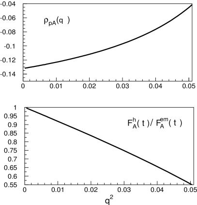
Figure 5: The upper panel: ratio of real to imaginary parts of the elastic amplitude for proton-carbon scattering calculated with Eq. (37). The bottom panel: Ratio of the hadronic and electromagnetic form factors as function of $t=-q^{2}$.

Note that $\rho_{pC}(q^{2})$ steeply decreases with $|t|$. As usual we employ the relation $B_{pA}\gg B$ for the proton which allows us to use in Eq. (37) the $pN$ $\rho$ value at $t=0$. The $t$-dependence of $\rho_{pC}$ shown in Fig. 5 is a result of nuclear effects. Likewise, the hadronic form factor is seen to drop off much faster than the em form factor. Both of these nuclear properties will be seen to have a significant effect on $A_{N}$, especially for the larger values of $q^{2}$ in this range.

Now we are in position to calculate the CNI asymmetry for elastic proton-nucleus scattering. First we calculate $A_{N}(t)$ assuming no hadronic spin-flip and fixing $\rho_{pC}=\delta_{pC}=0$. The result is depicted by dotted curve in Fig. 6.

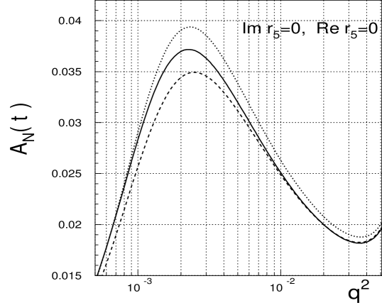
Figure 6: Asymmetry in polarized proton scattering on carbon in the Coulomb-nuclear region of momentum transfer. All curves are calculated using Eqs. (34)-(38) with $|r_{5}|=0$. The dotted curve corresponds to $\rho_{pC}=\delta_{pC}=0$. The dashed curve is calculated with $\rho_{pC}$ shown in Fig. 5 and $\delta_{pC}=0$. The solid curve includes effects of both $\rho_{pC}$ and $\delta_{pC}=0$.

The dashed curve includes $\rho_{pC}$ calculated with Eq. (38), but with $\delta_{pC}=0$. The solid curve shows the full calculation including both $\rho_{pC}$ and $\delta_{pC}$ calculated with Eq (38) and Eq (41). We keep ${\rm Re}~{}r_{5}=0$ in all calculations. We see that the asymmetry is quite sensitive to the values of both $\rho_{pC}$ and $\delta_{pC}$; however they contribute with opposite signs at small $t$ and partially cancel.

We next examine the behavior of $A_{N}(t)$ at larger $q^{2}$ including the region of the minimum in the hadronic form factor of $C^{12}$. This is shown in Fig. 7 for several reasonable values of $r_{5}$.

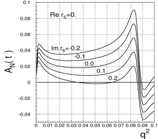
Figure 7: The same as in Fig. 6, with ${\rm Re}~{}r_{5}=0$, but ${\rm Im}~{}r_{5}=-0.2,\ -0.1,\ 0,\ 0.1,\ 0.2$. The $\rho_{pC}(q)$ and $\delta_{pC}(q)$ are included as calculated with Eqs. (38) and (41).

In spite of smallness of the Coulomb amplitude at such large $q^{2}$ the hadronic non-flip amplitude passes through zero near 0.09 GeV² and is equal to the electromagnetic near the zero position. This is why $A_{N}(t)$ reaches both a maximum and a minimum in this region.

Fig. 7 also shows that the asymmetry $A_{N}(t)$ is a sensitive function of ${\rm Im}~{}r_{5}$. This property was suggested in [15] as a unique way to measure the spin-flip part of the Pomeron amplitude. This value usually escapes observation since one does not expect a large phase shift between the spin-flip and non-flip part of the Pomeron amplitude. Such an experiment needs a polarized proton beam of known polarization (like in E950 experiment). On the other hand, if one needs to measure the polarization of a beam the unknown spin-flip hadronic amplitude can spoil the CNI method of polarimetry [21]. As soon as the E950 experiment at BNL provides information about $r_{5}$, one can use it for polarimetry at high energies at RHIC.

5. Summary

Proton-nucleus elastic scattering in the CNI region seems to be a better tool to measure the spin-flip part of the Pomeron amplitude than $pp$ because the main source of the spin-flip, the isovector Reggeons, is excluded (for an isoscalar nucleus like $C^{12}$) or suppressed by $1/A$. Therefore, one can perform measurements at rather low energies.

The observation made in this paper that the spin-flip fraction of the amplitude $\mu_{P}$ is nearly $A$-independent is very important for the method since it allows the application of results of measurements in $pA$ collisions to the $pp$ case. We have estimated the corrections to this statement caused by possible $t$-dependence of $\mu_{P}$ or by inelastic shadowing corrections and found these effects to be small.

We have predicted the asymmetry $A_{N}(t)$ at small $t$ in the kinematic region corresponding to the forthcoming data from the E950 experiment at BNL for proton-carbon elastic scattering with various assumptions about $\mu_{P}$. The real part of the $pC$ elastic amplitude and the Coulomb phase have been calculated and incorporated into our predictions. Comparison of E950 data is expected to provide the first determination of the spin properties of the Pomeron.

As soon as the spin-flip part of the Pomeron amplitude is known, one can use the CNI method as a reliable polarimeter for polarized proton beams at RHIC.

References

- [1] N.H. Buttimore, B.Z. Kopeliovich, E. Leader, J. Soffer, T.L. Trueman, Phys. Rev. D59, 114010 (1999).
- [2] N.H. Buttimore, E. Gotsman, E. Leader, Phys. Rev. D18 694 (1978).
- [3] R.J. Glauber, In: Lectures in Theor. Phys., v. 1, ed. W.E. Brittin and L.G. Duham. NY: Intersciences, 1959.
- [4] H. deVries et al, Nuc. Data Tables 36, 495 (1987).
- [5] H.A. Bethe, Ann. Phys. 3, 190 (1958).
- [6] H.S. Köhler, Nucl. Phys. 1, 433 (1956); I.I. Levintov, Doklady Akad. Nauk U.S.S.R. 107, 240 (1956); 30, 987 (1956) [Soviet Phys. JETP 3, 796 (1956)].
- [7] C. Bourrely, J. Soffer and D. Wray, Nucl. Phys. 87B, 32 (1975);91B, 33 (1975); C. Bourrely, E. Leader and D. Wray, Il Nuovo Cimento 35A, 559 (1976).
- [8] R.H. Bassel and C. Wilkin, Phys. Rev. 174, 1179 (1968).
- [9] V.N. Gribov, Sov. Phys. JETP 29, 483 (1969).
- [10] P.V.R. Murthy et al., Nucl. Phys. B92, 269 (1975).
- [11] B.Z. Kopeliovich and L.I. Lapidus, Pis’ma Zh. Eksp. Teor. Fiz., 28, 664 (1978) [Phys. JETP Lett. 28, 614 (1978)].
- [12] Al.B. Zamolodchikov, B.Z. Kopeliovich and L.I. Lapidus, Pis’ma Zh. Eksp. Teor. Fiz., 33, 612 (1981) [JETP Lett. 33, 565 (1981)].
- [13] V. Karmanov and L.A. Kondratyuk, Pis’ma Zh. Eksp. Teor. Fiz., 18, 179 (1973) [JETP Lett. 18, 266 (1973)].
- [14] B.Z. Kopeliovich, ’Polarisation Phenomena at High Energies and Low Momentum Transfer’, in Proc. of the Symposium ”Spin in high-energy physics”, ed. L.I. Lapidus, Dubna, 1982, p.97
- [15] B.Z. Kopeliovich and B.G. Zakharov, Phys. Lett. B226, 156 (1989).
- [16] Yu.M. Kazarinov, B.Z. Kopeliovich, L.I. Lapidus and I.K. Potashnikova, Zh. Eksp. Teor. Fiz., 70, 1152 (1976) [JETP 43, 598 (1976)].
- [17] B.Z. Kopeliovich, A. Schaefer, A.V. Tarasov, Phys. Rev. C59, 1609 (1999).
- [18] A. Schwimmer, Nuc. Phys. B94 445 (1975).
- [19] S. Bondarenko, E. Gotsman, E. Levin and U. Maor, hep-ph/0001260.
- [20] A.F. Martini and E. Predazzi, Pomeron contribution to Spin-flip, hep-ph/0012016
- [21] T.L. Trueman, CNI Polarimetry and the Hadronic Spin Dependence of pp Scattering, hep-ph/9610429
- [22] B.Z. Kopeliovich, High-Energy Polarimetry at RHIC, hep-ph/9801414
- [23] B.Z. Kopeliovich and L.I. Lapidus, Yad. Phys. 19, 218 (1974) [Sov. J. Nucl. Phys. 19, 114 (1974)].
- [24] R.N. Cahn, Z. Phys. C15, 253 (1982).
- [25] B.Z. Kopeliovich and A.V. Tarasov, Phys. Lett. B497, 44 (2001).
- [26] C. Bourrely and J. Soffer, Phys. Let. B442, 479 (1998).
- [27] I. Sick and J.S. McCarthy, Nucl.Phys. bf A150, 631 (1970).
- [28] E. Jenkins et al., Phys. Rev. Lett. 41, 217 (1978).