Energy Spectra of Reactor Neutrinos at KamLAND

Abstract

The upcoming reactor neutrino experiment, KamLAND, has the ability to explore the Large Mixing Angle (LMA) solution to the solar neutrino problem. Here, we investigate the precision to which KamLAND should be able to measure these parameters, utilizing the distortion of the energy spectrum of reactor neutrinos. Incomplete knowledge of the fuel composition of the reactors will lead to some error on this measurement. We estimate the size of this effect.

I Introduction

For a long time we have been aware that there is a deficit of neutrinos emanating from the sun. An apparent solution to this problem is the phenomenon of neutrino oscillations[1]. Particularly in light of the compelling atmospheric neutrino data from SuperKamiokande[2], we fully expect solar neutrinos to oscillate. Oscillations between two flavors can be described effectively by two parameters: the mass difference, $\Delta m^{2}$, and a mixing angle, $\tan^{2}\theta$. There are four regions in the $\Delta m^{2}$, $\tan^{2}\theta$ plane that explain the observed data on neutrinos from the sun. KamLAND is designed to explore one of these regions, the Large Mixing Angle (LMA) solution, through the detection of reactor neutrinos.

KamLAND [3] is an experiment to be located at the old Kamiokande site in the Kamioka mine in Japan. This location is of key importance to this experiment, as it is situated in the vicinity of 16 nuclear power plants which will contribute a significant neutrino flux. KamLAND consists of approximately 1 kiloton of liquid scintillator that will detect reactor neutrinos through the reaction:

$$p+\overline{\nu}_{e}\rightarrow n+e^{+}.$$ (1)

The positron is then detected when it scintillates and when it annihilates an electron. This annihilation, in delayed coincidence with the $\gamma$-ray from neutron capture, represents an easily recognizable signal.

In this letter, we assume that the solution to the solar neutrino problem is in the LMA region. We explore the accuracy to which the KamLAND experiment can utilize the reaction of Eq. (1) to measure the parameters of a LMA solution. In section II we review the basic procedure for computing the spectrum of neutrinos created at reactors. In section III, we review how to compute the expected number of events at KamLAND. In IV, we describe the results of an analysis of the energy spectrum of the detected neutrinos. Next, in section V we address the question of systematic errors associated with an incomplete knowledge of the incident neutrino spectrum. Finally, we conclude with a brief discussion of other possible systematics to be investigated. We also briefly mention some of the implications of this measurement for future neutrino experiments.

II Determination of Energy Spectrum

Because the mixing angle of $\nu_{e}$ in the mass gap responsible for the atmospheric neutrino oscillations is constrained to be small from CHOOZ reactor neutrino experiment [4], the solar and atmospheric oscillations decouple to a very good approximation. In this approximation, the important equation for the analysis of reactor neutrino oscillation becomes:

$$P(\overline{\nu}_{e}\rightarrow\overline{\nu}_{e})=1-\sin^{2}2\theta\,\sin^{2}\Bigl{(}\frac{1.27\Delta m^{2}(\mbox{eV${}^{2}$})L(\mbox{km})}{E(\mbox{GeV})}\Bigr{)}.$$ (2)

One of the advantages of the KamLAND design is that it is expected to have good energy resolution. An energy resolution of $\frac{\sigma(E)}{E}=\frac{10\%}{\sqrt{E}}$ or better is anticipated, where $E$ is measured in MeV [3]. As a result, if there are oscillations, one might hope to utilize the $E$ dependence of Eq. (2) to assist in making an accurate measurement of the oscillation parameters.

Of course, in order to take advantage of this energy dependence, one must have knowledge of the energy dependence of the incident neutrinos. That is to say, one is required to have a good knowledge of the unoscillated spectrum. We discuss the determination of this spectrum here.

A number of short baseline experiments [5] have measured the energy spectrum of reactors at distances where oscillatory effects should be completely negligible. A phenomenological parameterization of these spectra exists [6], which depends on the isotope involved. Namely, Vogel and Engel find that:

$$\frac{dN_{\nu}}{dE_{\nu}}=e^{a_{0}+a_{1}E_{\nu}+a_{2}E_{\nu}},$$ (3)

where the fitted values of the parameters $a_{i}$ are reproduced from [6] in Table I. This spectrum is given in units of $\frac{\overline{\nu}_{e}}{\rm MeV-fission}$. Therefore, given this spectrum, it remains to determine how many fissions of each isotope there are. For a given reactor site, this will depend on three factors:

1. The thermal power of that reactor.

2. The isotopic composition of the reactor fuel.

3. The amount of thermal power emitted during the fissioning of a nucleus of a given isotope.

.

TABLE I.: Parameters for $\frac{dN_{\nu}}{dE_{\nu}}$ parameterization. The resulting spectrum is given in units of $\overline{\nu}_{e}$/MeV-fission.

Isotope	235U	239Pu	238U	241Pu
$a_{0}$	0.870	0.896	0.976	0.793
$a_{1}$	-0.160	-0.239	-0.162	-0.080
$a_{2}$	-0.0910	-0.0981	-0.0790	-0.1085

FIG. 1.: The time dependent composition of reactor fuel. Taken from reference [9].

For convenience, we reproduce the relevant reactor characteristics in Table II. The maximum thermal power is given in the table. This addresses the first point above. Isotopic composition is a somewhat complicated issue, and we will investigate it more fully in section V. For the present, let us simply note that, in general, the time composition of the fuel varies roughly as in Fig. 1. For the analysis of section IV, we take all reactors as having a composition varying as in this figure. We assume that at the end of the 7 month cycle shown, the composition reverts back initial levels (refueling). Finally, for point three, we note that the thermal energy, $\epsilon_{i}$ associated with the fissioning of a given nucleon is known [7]. The relevant values are displayed in Table III. With these pieces of information, we are able to determine the neutrino spectrum emitted from each reactor, $S(i,t,E)$. Here, $i$ labels the reactor.

TABLE II.: Reactor parameters. Reproduced from reference [3].

Reactor Site	Distance (km)	Max. Thermal Power (GW)
Kashiwazaki	160	24.6
Ohi	180	13.7
Takahama	191	10.2
Hamaoka	213	10.6
Tsuruga	139	4.5
Shiga	81	1.6
Mihama	145	4.9
Fukushima-1	344	14.2
Fukushima-2	344	13.2
Tokai-II	295	3.3
Shimane	414	3.8
Ikata	561	6.0
Genkai	755	6.7
Onagawa	430	4.1
Tomari	784	3.3
Sendai	824	5.3

TABLE III.: Energy per fission of isotopes that make significant contributions to the thermal power of a reactor.

Fissioning Isotope	235U	239Pu	238U	241Pu
Energy Per Isotope (MeV)	201.7	205.0	210.0	212.4

III Determination of Expected Number of Events

Now that we have the initial spectrum in hand, we review how one finds the expected number of events at KamLAND. To determine the number of neutrinos detected at KamLAND, one must convolve the cross section, $\sigma(E_{v})$, for the reaction shown in Eq. (1) with the reactor spectra, $S(i,t,E)$. To lowest order the cross section is [10]:

$$\sigma(E_{\nu})=\frac{2\pi^{2}}{m_{e}^{5}f\tau_{n}}p_{e}E_{e}.$$ (4)

Here $f=1.69$ is the integrated Fermi function for neutron $\beta$-decay, $m_{e}$ is the mass of the electron, $E_{e}$ is the electron energy, and $p_{e}$ is the electron momentum. The energy of the electron, to lowest order, is given by [10]:

$$E_{e}=E_{\nu}-1.293\;\mbox{MeV}.$$ (5)

That is to say, the energy of the electron is basically the energy of the incident neutrino minus the proton-neutron mass difference. In our numerical calculations, we used the cross section which takes into account the nucleon recoil, which may be found in [11].

The expected number of events at KamLAND is given by:

$$N(t,E_{\nu},\Delta m^{2},\sin^{2}2\theta)$$ (7)

$$=\sum_{i}\frac{S(i,t,E_{\nu})}{4\pi d_{i}^{2}}\sigma(E_{\nu})P(\Delta m^{2},\sin^{2}2\theta).$$

Here, $P$ is the probability from Eq. (2), $\sigma(E_{\nu})$ is the full cross section analogous to Eq. (5), and $S(i,t,E_{\nu})$ is the initial energy spectrum, to be calculated as described above. The values of the distances can also be found in Table II.

IV Results

With the expected number of events in hand, it is only a matter of a simple $\chi^{2}$ analysis to fit for the oscillation parameters. In this section, we ignore background effects. To estimate the precision to which KamLAND could measure the oscillation parameters, we assumed a 3 kt-year exposure where all reactors operated at 78% of their maximum capacity. It was assumed that the fuel composition of each reactor varied as shown in Fig. 1. Perfect detector efficiency was assumed. To lowest order, this is not a bad assumption, given the recognizable delayed coincidence signal. The measurements that KamLAND could be expected to perform with these assumptions are shown in Fig. 2. Contours were generated by finding the minimum $\chi^{2}$, and then calculating the confidence levels for two degrees of freedom ($\tan^{2}\theta$ and $\Delta m^{2}$). Data were binned in $0.5$ MeV bins. The fit was done for visible energies between $E_{\it visible}=1.22$ MeV and $E_{\it visible}=7.0$ MeV. The first bin is smaller, since our parameterization of the incident spectra is only good above $E_{\nu}=2$ MeV. The cutoff at high energies is to avoid the low statistics bins, where there is not much statistical discrimination, and Poisson statistics would be necessary.

Since the oscillations in this case depend on the mixing angle only through $\sin^{2}2\theta$, there is a two-fold degeneracy in the measurement (hence the reflection symmetry about $\tan^{2}\theta=1$). However, the LMA solution, which is overlayed, does not posses such a symmetry, so it is necessary to plot against $\tan^{2}\theta$ and not $\sin^{2}2\theta$ [12].

From the figure, it is clear that KamLAND is able to make a very accurate measurement of the $\Delta m^{2}$ parameter in particular. To see why this is so, it is instructive to look at the quantity:

$$R=\frac{\#\mbox{Observed}}{\#\mbox{No Oscillation}}.$$ (8)

Plots of this quantity are shown in Fig. 3. This should essentially be the oscillation probability. By determining the position of the dip in the oscillation, one is able to determine the value of $\Delta m^{2}$. From the figure, one can see that the location of the dip can be well determined by KamLAND if the oscillations parameters lie in the LMA solution to the solar neutrino problem.

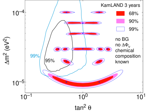
FIG. 2.: The expected measurement of $\Delta m^{2}$ and $\tan^{2}\theta$. Contours for 68%, 90% and 99% CL are shown.The LMA solution to the solar neutrino problem is overlayed [8].

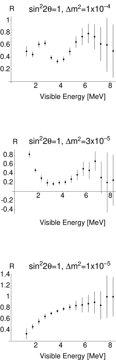
FIG. 3.: The ratio, R, of the number of events seen, to the number of events expected if there were no oscillations. The error bars are statistical.

V Fuel Composition Effects

Let us now address the question of the effect of the fuel composition. To calculate the evolution of the different components of reactor fuel is a complicated business. KamLAND expects to obtain the time dependent compositions from the power companies involved. This section serves to demonstrate that this is an important piece of information for this experiment.

To estimate the effect that an incomplete knowledge of the fuel composition would have on the measurement, we took the extreme cases. We look at the neutrino spectrum that would result from taking the composition to be as illustrated in Fig. 2, we refer to this as the “true composition.” We then tried to fit the observed data that were generated from the true composition with the expected number of events from three different compositions:

1. The true composition,

2. A composition that stays constant and equal to the composition at $t=0$,

3. A composition that stays constant and equal to the composition at $t=220$ days.

The different spectra are shown in Fig. 4. Although the basic shapes are relatively consistent, there are important differences, as can be seen by examining Fig. 5, where we plot the difference between the spectra, normalized to the average spectrum. At the higher energies, differences in the initial and final spectra can reach over 15%.

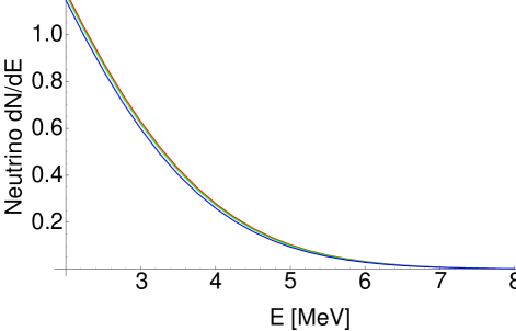
FIG. 4.: Neutrino spectra generate using the initial, final and average fuel composition.Although the differences here are somewhat difficult to discern, they are move easily visible in Fig. 5.

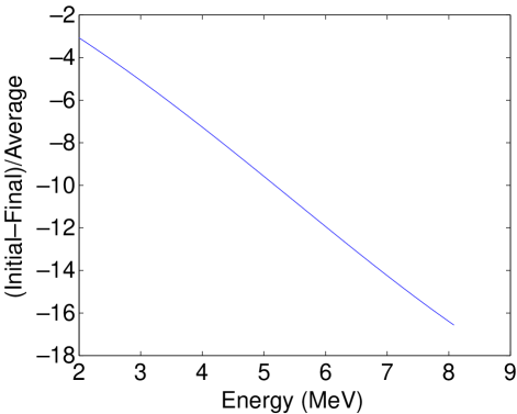
FIG. 5.: Here we have plotted the percentage difference in the initial and final spectra. More precisely, we have plotted the 100 times the difference between the initial and final spectra, divided by the average spectrum.

The difference between the three fits done in this way should give an estimate of the systematic error involved. A contour plot showing the measurements in the ($\tan^{2}\theta$, $\Delta m^{2}$) plane is shown in Fig. 6. Although the values of the measured quantities are not drastically affected, particularly in the cases of moderate $\Delta m^{2}$, fuel composition clearly is an important systematic error to be considered. It is also of interest to see how incorrect assumptions about fuel composition degrades the fit. We show the $\chi^{2}$ for 10 degrees of freedom in Table IV. In particular, the $\chi^{2}$ is not nearly as good for the fits with the final spectrum.

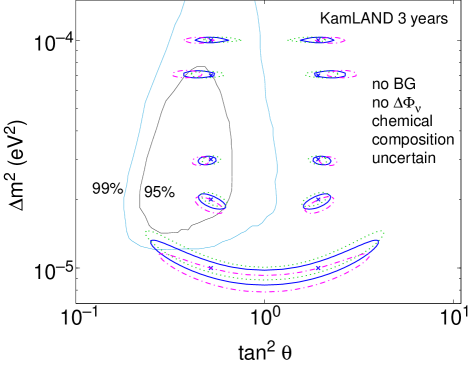
FIG. 6.: 90 % confidence level contours for measurements of $\Delta m^{2}$ and $\tan^{2}\theta$. The contours were generated by varying the assumptions about the composition of the fuel. For further explanation, see the text.

TABLE IV.: The fits corresponding to three different fuel compositions. For each point in ($\Delta m^{2}$,$\tan^{2}\theta$) space, the events incident on KamLAND were generated with a time dependent (T) composition. Fits were done with the time dependent (T), initial (I), and final (F), composition.

Comp.	$\Delta m^{2}$	$\tan^{2}\theta$	Fit $\Delta m^{2}$	Fit $\tan^{2}\theta$	$\chi^{2}$ (10 dof)
T	$1\times 10^{-5}$	0.52, 1.92	$9.5\times 10^{-6}$	0.64, 1.55	12.89
I	$1\times 10^{-5}$	0.52, 1.92	$1.1\times 10^{-5}$	0.43, 2.30	9.64
F	$1\times 10^{-5}$	0.52, 1.92	$8.7\times 10^{-6}$	0.80, 1.24	21.67
T	$2\times 10^{-5}$	0.52, 1.92	$1.9\times 10^{-5}$	0.54, 1.87	12.42
I	$2\times 10^{-5}$	0.52, 1.92	$2.0\times 10^{-5}$	0.53, 1.87	9.50
F	$2\times 10^{-5}$	0.52, 1.92	$1.9\times 10^{-5}$	0.50, 2.01	18.26
T	$3\times 10^{-5}$	0.52, 1.92	$3.0\times 10^{-5}$	0.50, 2.01	12.17
I	$3\times 10^{-5}$	0.52, 1.92	$3.0\times 10^{-5}$	0.51, 1.94	10.2
F	$3\times 10^{-5}$	0.52, 1.92	$3.0\times 10^{-5}$	0.46, 2.16	16.19
T	$7\times 10^{-5}$	0.52, 1.92	$7.2\times 10^{-5}$	0.45, 2.23	10.73
I	$7\times 10^{-5}$	0.52, 1.92	$7.0\times 10^{-5}$	0.50, 2.01	11.96
F	$7\times 10^{-5}$	0.52, 1.92	$7.2\times 10^{-5}$	0.39, 2.58	11.57
T	$1\times 10^{-4}$	0.52, 1.92	$1.0\times 10^{-4}$	0.51, 1.94	12.96
I	$1\times 10^{-4}$	0.52, 1.92	$1.0\times 10^{-4}$	0.58, 1.72	8.58
F	$1\times 10^{-4}$	0.52, 1.92	$1.0\times 10^{-4}$	0.45, 2.23	21.87

VI Flux Uncertainty Effects

Finally, we relax our assumption that KamLAND will have complete knowledge of the overall flux normalization. We assume that the flux is known with a three percent error, consistent with the size of the errors in the $\beta$-spectroscopy experiment at the Gösgen reactor [9]. We then can compute a $\chi^{2}$, that takes this uncertainty into account. In particular, we write:

$$\chi^{2}={\rm min}\left(\chi^{2}_{bins}+\frac{(N-1.0)^{2}}{\sigma_{N}^{2}}\right).$$ (9)

Here, $\sigma_{N}^{2}=.03^{2}$. We vary the possible normalizations, $N$, and take the minimum of the right hand side. Of course, the $\chi^{2}_{bins}$ is a function of $N$ as well, as the theoretical prediction depends on the incident flux. Note, in general, this procedure will provide a smaller $\chi^{2}$, at each set of oscillation parameters, resulting in larger contours. From Fig. 7, we can see that the contours are enlarged slightly. In particular, the uncertainty in the overall flux causes a slight degradation of the measurement of the mixing angle. This is a well-known and important effect. For completeness, we tabulate the values of $\chi^{2}$ in Table V.

TABLE V.: The fits corresponding to three different fuel compositions. For each point in ($\Delta m^{2}$,$\tan^{2}\theta$) space, the events incident on KamLAND were generated with a time dependent composition. Fits were done either allowing the overall flux to float (Float), or keeping it fixed at the predicted value. (Fixed).

Comp.	$\Delta m^{2}$	$\tan^{2}\theta$	Fit $\Delta m^{2}$	Fit $\tan^{2}\theta$	$\chi^{2}$ (10 dof)
Fix	$1\times 10^{-5}$	0.52, 1.92	$9.5\times 10^{-6}$	0.56, 1.55	12.89
Float	$1\times 10^{-5}$	0.52, 1.92	$1.0\times 10^{-5}$	0.56, 1.79	12.38
Fix	$2\times 10^{-5}$	0.52, 1.92	$1.9\times 10^{-5}$	0.54, 1.87	12.42
Float	$2\times 10^{-5}$	0.52, 1.92	$2.0\times 10^{-5}$	0.54, 1.87	12.06
Fix	$3\times 10^{-5}$	0.52, 1.92	$3.0\times 10^{-5}$	0.50, 2.01	12.17
Float	$3\times 10^{-5}$	0.52, 1.92	$3.0\times 10^{-5}$	0.51, 1.94	11.88
Fix	$7\times 10^{-5}$	0.52, 1.92	$7.2\times 10^{-5}$	0.45, 2.23	10.73
Float	$7\times 10^{-5}$	0.52, 1.92	$7.0\times 10^{-5}$	0.61, 1.63	9.74
Fix	$1\times 10^{-4}$	0.52, 1.92	$1.0\times 10^{-4}$	0.51, 1.94	12.96
Float	$1\times 10^{-4}$	0.52, 1.92	$1.0\times 10^{-4}$	0.58, 1.71	11.71

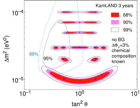
FIG. 7.: The contours that arise from including the flux uncertainty in the $\chi^{2}$.

VII Experimental Systematics

Although we are not in a position to make a quantitative study of the experimental systematics at KamLAND, a few brief comments are possible. First of all, in the preceding analysis, we have neglected the contribution from the backgrounds. In the reactor experiment, there is a distinctive delayed neutron-capture signature, which results in a substantial reduction of backgrounds. The background level was conservatively estimated to be 20:1 [3] (i.e., probably an overestimate). It is not so unreasonable to ignore the backgrounds. Moreover, one expects that backgrounds will be a relatively steeply falling function of energy. So, if the energy where the interesting oscillation effects occur is high enough, then the assumption of no backgrounds is even safer. This happens at the larger $\Delta m^{2}$ values, as can clearly be seen from Eqn. (2). In addition, KamLAND hopes to get a handle on the backgrounds by utilizing the fact that power usage, and hence neutrino flux, varies seasonally [3]. The amount of power produced over time will be available from the power companies.

We would like to briefly mention other possible sources of systematic uncertainties. As mentioned earlier in the paper, there is an issue of the energy resolution of the detector. This could smear out the location of the “dip” that is so nicely seen, in Fig. 3(a). However, the resolution expected is better than the size of the bins and hence is not expected to affect the results. A more difficult issue would be to accurately callibrate the energy measurement of the detector of this size. There are plans to do so; see [3]. There will be a source of backgrounds from geological neutrinos in the 2-3 MeV region which may or may not be important. However, a simple energy cut should remove them completely.

VIII Conclusions

The KamLAND reactor neutrino experiment should allow for an accurate measurement of $\Delta m^{2}$, as long as the solution to the solar neutrino problem is in the LMA region. Incomplete knowledge of the fuel composition at the reactors will represent an important source of experimental error. In this letter, we assumed perfect detector efficiency, and that backgrounds were well understood. It is interesting to note that the precision to which KamLAND is able to measure $\Delta m^{2}$ may effect the ability of a muon source neutrino factory to extract information about the CP violating phase in the MNS matrix. CP violation is an phenomenon that requires at least three generations, the effects of the sub-leading oscillation is crucial, and the matter effect needs to be accurately subtracted in order to determine $\delta_{CP}$. The measurements at KamLAND should prove crucial for this purpose.

IX Acknowledgements

This was supported in part by the Director, Office of Science, Office of High Energy and Nuclear Physics, Division of High Energy Physics of the U.S. Department of Energy under Contract DE-AC03-76SF00098 and in part by the National Science Foundation under grant PHY-95-14797. AP is also supported by a National Science Foundation Graduate Fellowship.

Note Added

During the final preparation of this manuscript, we became aware of papers on a similar topic [13, 14]. Both of them discussed how accurately KamLAND will determine the oscillation parameters. Ref. [13] further included the three-generation mixing effects, while Ref. [14] studied $\Delta m^{2}>2\times 10^{-4}$ eV² as well. Neither of them discusses the effect of fuel composition and overall flux normalization quantitatively, however. Other conclusions appear to be consistent.

REFERENCES

- [1] Z. Maki, M. Nakagawa, and S. Sakata, Prog. Theor. Phys. 28, 870 (1962). B. Pontecorvo. Zh. Eksp. Teor. Fiz. 52, 1717 (1967).
- [2] Super-Kamiokande Collaboration (Y. Fukuda et al.), Phys. Lett. B B436, 33 (1998).
- [3] “Proposal for US Participation in KamLAND,” March 1999, http://kamland.lbl.gov/KamLAND.US.Proposal.pdf
- [4] M. Apollonio et al. Phys. Lett. B466, 415 (1999) [hep-ex/9907037].
- [5] A.A. Hahn et al.Phys. Lett. B 218, 365 (1989). K. Schreckenbach et al.Phys. Lett. B 160, 325 (1985).
- [6] P. Vogel and J. Engel. Phys. Rev. D 39, 3378 (1989).
- [7] F. Boehm and P.Vogel. The Physics of Massive Neutrinos. (New York: Cambridge University Press) 1992.
- [8] LMA contour taken from C. Gonzalez-Garcia at http://ific.uv.es/∼penya/2nu.html.
- [9] G. Zacek, et al., Phys. Rev. D 34, 2621 (1986).
- [10] P. Vogel. Phys. Rev. D 29, 1918 (1984).
- [11] P. Vogel. and J.F. Beacom. Phys. Rev. D 60, 053003 (1999).
- [12] A. de Gouvea, A. Friedland and H. Murayama. Phys. Lett. B490, 125 (2000) [hep-ph/0002064].
- [13] V. Barger, D. Marfatia, and B. Wood. hep-ph/0011251.
- [14] R. Barbieri and A. Strumia, hep-ph/0011307.