Abstract

Lattice measurements of the Pisa group (A.Di Giacomo et al., hep-lat/9603018) are analyzed numerically and parameters of correlation functions are extracted from the data – both below and above deconfinement temperature $T_{c}$. Gluon condensate is found for six temperatures in the interval 0.956 $T_{c}$ – 1.131 $T_{c}$ and field distributions in deconfined phase are obtained.

1 Introduction

Study of field distributions around static quarks has a long history. The information obtained both analytically and on the lattice has an important meaning in several respects. Firstly, it demonstrates clearly the appearance of the QCD string between the charges in the confining phase and the detailed contents of the fields in this string; e.g., the string consists mainly of longitudinal color-electric field. Secondly, since the string enters in many dynamical quantities, such as static interquark potential, spin-dependent forces for heavy quarkonia etc., one can easily compute these quantities from the string field distributions.

Finally, and this is the purpose of the present paper, the phenomenon of deconfinement is not fully understood from the point of view of the string and field distributions.

What actually happens when temperature $T$ exceeds the critical value – the string disappears or distribution of fields drastically change, so that to compensate the string tension?

Happily there exist numerical lattice measurements of field correlators near the critical temperature $T_{c}$, made by the Pisa group [1], where both electric and magnetic correlators are found with good accuracy. These data clearly demonstrate the strong suppression of color-electric component above $T_{c}$ and persistence of color-magnetic components.

The purpose of the present paper is twofold. First, we reanalyze the data of [1] in terms of correlators $D^{\mathrm{E,B}}$ and $D_{1}^{\mathrm{E,B}}$ which are better understood from the point of view of perturbative and nonperturbative contributions [2]. There was e.g. shown that the string tension $\sigma$ (”conventional” electric or ”spatial” magnetic) is expressed directly through the $D^{\mathrm{E,B}}$ but not the $D_{1}^{\mathrm{E,B}}$. Given the simple assumption of behavior $D^{\mathrm{E,B}}(x)$ and $D_{1}^{\mathrm{E,B}}(x)$ in all region of distances $x$ between correlation points, we obtain the behavior of gluon condensate near the $T_{c}$ (which is defined by $D^{\mathrm{E,B}}(0)$ and $D_{1}^{\mathrm{E,B}}(0)$). Second, using the obtained $D^{\mathrm{E,B}}(x)$ and $D_{1}^{\mathrm{E,B}}(x)$, we calculate the color field distributions around static quarks in the deconfined phase. We perform these calculations using the connected probe [3] in the framework of Field Correlator Method (FCM) [4,5]. We study in detail two possible from the deconfinement point of view regimes, corresponding to two forms of $D(x)$, extracted from lattice data [1]. In the first one the string disappears and in the second (less appealing physically, but more supported by the lattice data) the string becomes a coaxial cable with the empty core.

The paper is organized as follows.

In Section 2 a short description is given of our fitting procedure of magnetic correlators at any $T$ and the electric correlators at $T<T_{c}$, while in Section 3 more prolonged one is given for electric correlators at $T>T_{c}$. The Section 4 is devoted to the behaviour of the gluonic condensate below and above $T_{c}$. In Section 5 the detailed equations for the field distributions around deconfined quark and antiquark are given and illustrated graphically. In the concluding section results of the paper are summarized and discussed.

2 Fitting data with nonzero string tension

In this section we consider magnetic correlators in all temperature region and electric correlators at $T<T_{c}$ since both of them produce (e.g., spatial) nonzero string tension. We fit the data [1] using the method of least squares [6]. To begin with, we express the functions $D_{||}(x),~{}D_{\bot}(x)$ through the $D(x),~{}D_{1}(x)$ and represent the lasts as sums of nonperturbative (NP) and perturbative (P) (diverging at zero) contributions. This is the procedure used by A.Di Giacomo et al.[7] when analyzing the correlation functions at zero temperature. The difference is that we should distinguish electric and magnetic correlators due to the fact that the finite temperature theory has only the $O(3)\times O(1)$ symmetry.

We fit distributions of

$$D_{||}^{\mathrm{E,B}}(x)=D^{\mathrm{E,B}}(x)+D_{1}^{\mathrm{E,B}}(x)+\frac{x}{2}\frac{\partial D_{1}^{\mathrm{E,B}}(x)}{\partial x}$$ (1)

and

$$D_{\bot}^{\mathrm{E,B}}(x)=D^{\mathrm{E,B}}(x)+D_{1}^{\mathrm{E,B}}(x)$$ (2)

electric and magnetic correlation functions in the range from 0.4 to 1 fm. All points are measured at $x_{4}=0$. In this section we parameterize the functions as follows:

$$D(x)=A\exp(-x/\lambda_{A})+\frac{a}{x^{4}}\exp(-x/\lambda_{a}),$$ (3)

$$D_{1}(x)=B\exp(-x/\lambda_{B})+\frac{b}{x^{4}}\exp(-x/\lambda_{b}).$$ (4)

Fitting the magnetic functions (which are close to exponentials), we set in (3),(4) $\lambda_{a}=\lambda_{b}=\lambda_{B}$, thus using $k=6$ fitting parameters. Given $N=12$ number of data, we have as a result $n=N-k=6$ number of degrees of freedom. The results are shown in Table 1. One-standard-deviation errors $\Delta\alpha_{i}$ are determined from the equation $\chi^{2}(\alpha_{1},...,\alpha_{i}+\Delta\alpha_{i},...,\alpha_{k})=\chi^{2}(\alpha_{1},...,\alpha_{i},...,\alpha_{k})+\Delta\chi^{2}_{k}$, where $\alpha_{i}$ are fitted parameters and $\Delta\chi^{2}_{1}=1$, $\Delta\chi^{2}_{4}=4.75$, $\Delta\chi^{2}_{6}=7$ [6].

Preliminary fitting of electric data at $T=0.956T_{c}$ with parameters of (3),(4) gave unacceptable big $\chi^{2}$ due to the end points of $D^{\mathrm{E}}_{||}$ and $D^{\mathrm{E}}_{\bot}$; $\lambda_{A},~{}\lambda_{a}$, and $\lambda_{b}$ were found close to each other. Therefore we had removed mentioned points and set $\lambda_{A}=\lambda_{a}=\lambda_{b}$ to get the reasonable fit (Table 2).

Preliminary fitting of electric data at $T=0.978T_{c}$ have shown that $\chi^{2}$ is also too big and besides that $\lambda_{A}$ is close to $\lambda_{b}$ and $\lambda_{B}$ to $\lambda_{a}$. Therefore we set $\lambda_{b}=\lambda_{A}$ and $\lambda_{a}=\lambda_{B}$. To improve $\chi^{2}$, we enlarge two times the error of the last point of $D_{||}^{E}$ (Fig. 1). One can make sure from Figure 1 that this point is largely off the exponential curve, which may be connected to the lattice size effects. The results of fitting are shown in Table 2.

3 Fitting electric data in the deconfinement region

$D^{\mathrm{E}}_{||}$ above $T_{c}$ has a drop that is presumably related with the deconfinement transition, when the string tension of area law asymptotics of Wilson loop for static quarks disappears. In gaussian approximation of FCM [5] we get

$$\sigma=\frac{1}{2}\int dx_{1}dx_{4}D^{\mathrm{E,NP}}(x_{1},x_{4})=0.$$ (5)

In this region we should alter the form of $D$ (3) to justify (5). It is naturally to set

$$D^{\mathrm{NP}}(x)\equiv 0.$$ (6)

(We omit subscript ”E” here and in what follows in this section.) As we shall see below, this form assures reasonably well fit of data. Let us propose another form of $D$ to ensure good fitting of data. We suppose now more constrained $O(4)$ symmetry: $D(\mbox{\boldmath${\rm x}$}^{2},x_{4}^{2})=D(\mbox{\boldmath${\rm x}$}^{2}+x_{4}^{2})\equiv D(x^{2})$ to get

$$\sigma=\frac{\pi}{2}\int_{0}^{\infty}dx^{2}D^{\mathrm{NP}}(x^{2})=\frac{\pi}{2}\int_{0}^{\infty}dx^{2}D^{\mathrm{NP}}_{||}(x^{2})=0.$$ (7)

To better reproduce the mentioned drop of data, we set $D^{\mathrm{NP}}_{||}(x)\equiv 0$, i.e.,

$$D^{\mathrm{NP}}(x)=-D_{1}^{\mathrm{NP}}(x)-\frac{x}{2}\frac{\partial D_{1}^{\mathrm{NP}}(x)}{\partial x},$$ (8)

leaving meanwhile $D_{1}$ in form (4) intact.

So far we have adopted two forms of $D(x)$:

$$D(x)=\frac{a}{x^{4}}\exp(-x/\lambda_{a});$$ (9)

$$D(x)=B(\frac{x}{2\lambda_{B}}-1)\exp(-x/\lambda_{B})-\frac{a}{x^{4}}\exp(-x/\lambda_{a}).$$ (10)

We fit data on $D_{||}$ and $D_{\bot}$ at $T=1.011T_{c}$ in two ways, using (a): functions (9),(4) and (b): (10),(4). Having in mind the small number of data we set $\lambda_{a}=\lambda_{b}=\lambda_{B}$ to have $k=4$. Given $N=9$, we obtain $n=5$ (Table 3). We see from the Table 3 the somewhat reasonable $\chi^{2}/n=1.7$ in case (a) and excellent $\chi^{2}/n=1.05$ in case (b).

At higher temperatures there are only two measurements of $D_{||}$, with values significantly less even than the errors of corresponding points of $D_{\bot}$. This circumstance allows us to subdivide the fitting procedure in two stages. At the first stage we fit the difference $D_{\bot}-D_{||}$ (cf. (1),(2)) by $-x^{2}\partial D_{1}/\partial x^{2}$ (cf. (4)), and extract parameteres ($B,\lambda_{B},b,\lambda_{b}$). At the second stage we fit $D_{\bot}$, reproducing it (in two ways, due to two cases of $D$) by the sum of $D$ and $D_{1}$ with parameters extracted from the first fit; $D$ is taken in forms (9) and (10) with $\lambda_{a}=\lambda_{b}$ in both cases, and only parameter $a$ is allowed to vary (Table 4, Fig. 2). One-standard-deviation errors are determined as described above, with $k=4$ at the first stage and $k=1$ at the second stage of fitting. In the Table 4 the second–stage–fitting results are separated by horizontal line; $\chi_{1,2}^{2}$ refer to the first and second stages correspondingly.

As $D_{\bot}-D_{||}\approx D_{\bot}$, at the first stage we actually fit the data by

$$D_{\bot}(x)=\frac{Bx}{2\lambda_{B}}\exp(-x/\lambda_{B})+\frac{2b}{x^{4}}(1+\frac{x}{4\lambda_{b}})\exp(-x/\lambda_{b})$$ (11)

and at the second stage in case (a) by

$$D_{\bot}(x)=B\exp(-x/\lambda_{B})+\frac{a+b}{x^{4}}\exp(-x/\lambda_{b})$$ (12)

and in case (b) by

$$D_{\bot}(x)=\frac{Bx}{2\lambda_{B}}\exp(-x/\lambda_{B})+\frac{a+b}{x^{4}}\exp(-x/\lambda_{b}),$$ (13)

with all parameters of (12),(13) except $a$ fixed by the first stage. One could see that (13) well reproduces (11) at $a=b$ and any $B$ and $\lambda_{B}$, for $x\ll 4\lambda_{b}$, i.e., in all measured region $0.4$ fm$<x<1$ fm (see Table 4).

4 Temperature dependence of the gluon condensate

The gluon condensate is defined as

$$G_{2}=\frac{\alpha_{s}}{\pi}\langle F_{\mu\nu}^{a}F_{\mu\nu}^{a}\rangle,$$ (14)

where $\alpha_{s}$ is the strong coupling constant, $F_{\mu\nu}^{a}$ are the gauge field strengths taken at the point $x=0$ and the averaging is performed over all vacuum configurations. At zero temperature the FCM reads

$$\frac{g^{2}}{N_{c}}\langle F_{\rho\sigma}^{a}(x^{\prime})(T^{a})^{\alpha}_{\beta}\Phi^{\beta}_{\gamma}(x^{\prime},x)F_{\mu\nu}^{b}(x)(T^{b})^{\gamma}_{\delta}\Phi^{\delta}_{\alpha}(x,x^{\prime})\rangle=$$

$$(\delta_{\rho\mu}\delta_{\sigma\nu}-\delta_{\rho\nu}\delta_{\sigma\mu})(D(h^{2})+D_{1}(h^{2}))+$$

$$(h_{\mu}h_{\rho}\delta_{\nu\sigma}-h_{\mu}h_{\sigma}\delta_{\nu\rho}-h_{\rho}h_{\nu}\delta_{\mu\sigma}+h_{\nu}h_{\sigma}\delta_{\mu\rho})\frac{\partial D_{1}(h^{2})}{\partial h^{2}},$$ (15)

where $h\equiv x-x^{\prime}$;  $\alpha$,…,$\delta$ are color indices. At $x=x^{\prime}=0$ one uses in (15) $\mathrm{tr}T^{a}T^{b}=\frac{1}{2}\delta^{ab}$ and gets

$$\frac{g^{2}}{2N_{c}}\langle F_{\mu\nu}^{a}F_{\mu\nu}^{a}\rangle=12(D(0)+D_{1}(0)).$$ (16)

In what follows we shall use the zero temperature lattice results [7]:

$$D^{\mathrm{NP}}(0)=3.3\times 10^{8}\Lambda^{4}_{L}=129~{}\mathrm{fm}^{-4},~{}D_{1}^{\mathrm{NP}}(0)=0.7\times 10^{8}\Lambda^{4}_{L}=27~{}\mathrm{fm}^{-4},$$ (17)

where $\Lambda_{L}=0.025$ fm^-1 is the fundamental constant of QCD in lattice renormalization scheme; its value is extracted from the string tension.

At finite temperature one derives from (15)

$$\frac{g^{2}}{2N_{c}}\langle E_{i}^{a}(0)E_{i}^{a}(0)\rangle=3(D^{\mathrm{E}}(0)+D_{1}^{\mathrm{E}}(0)),$$ (18)

$$\frac{g^{2}}{2N_{c}}\langle B_{i}^{a}(0)B_{i}^{a}(0)\rangle=3(D^{\mathrm{B}}(0)+D_{1}^{\mathrm{B}}(0)),$$ (19)

where $E_{i}\equiv F_{0i}$ and $B_{i}\equiv\frac{1}{2}\epsilon_{ilm}F_{lm}$. Note that at finite temperature $D^{\mathrm{E}}$ and $D^{\mathrm{B}}$ acquire subscripts for symmetry breaking $O(4)\longrightarrow O(3)\times O(1)$ reason. We have to distinguish electric and magnetic contributions to condensate:

$$\langle F_{\mu\nu}^{a}F_{\mu\nu}^{a}\rangle=\langle F^{2}\rangle_{\mathrm{el}}+\langle F^{2}\rangle_{\mathrm{magn}},$$ (20)

where

$$\langle F^{2}\rangle_{\mathrm{el}}\equiv\langle F_{0i}^{a}F_{0i}^{a}\rangle+\langle F_{i0}^{a}F_{i0}^{a}\rangle=2\langle E_{i}^{a}E_{i}^{a}\rangle,$$ (21)

$$\langle F^{2}\rangle_{\mathrm{magn}}\equiv\frac{1}{4}\epsilon_{ijk}\epsilon_{ijk}\langle F_{jk}F_{jk}\rangle+\frac{1}{4}\epsilon_{ijk}\epsilon_{ijk}\langle F_{kj}F_{kj}\rangle=2\langle B_{i}^{a}B_{i}^{a}\rangle$$ (22)

Substituting (16), (18)–(22) into (14), one obtains that normalized gluonic condensate is

$$\frac{G_{2}(T)}{G^{0}_{2}}=\frac{D^{\mathrm{E,NP}}(0)+D_{1}^{\mathrm{E,NP}}(0)+D^{\mathrm{B,NP}}(0)+D_{1}^{\mathrm{B,NP}}(0)}{2(D(0)+D_{1}(0))},$$ (23)

where $G_{2}(T)$ is the gluon condensate at temperature $T$; $G^{0}_{2}\equiv G_{2}(0)$.

According to our fitting, magnetic condensate is $D^{\mathrm{B,NP}}(0)+D_{1}^{\mathrm{B,NP}}(0)=A+B$, with $A,B$ taken from Table 1. Electric condensate at temperature $T<T_{c}$ is $D^{\mathrm{E,NP}}(0)+D_{1}^{\mathrm{E,NP}}(0)=A+B$, with $A,B$ taken from Table 2. At $T>T_{c}$ in case (a) $D^{\mathrm{E,NP}}(0)=0$, $D_{1}^{\mathrm{E,NP}}(0)=B$, with $B$ taken from Tables 3,4, and in case (b) $D^{\mathrm{E,NP}}(0)+D_{1}^{\mathrm{E,NP}}(0)=0$.

The behavior of the condensate and that of its electric and magnetic constituents with temperature are shown in Tables 5,6. Data on the whole condensate from these Tables are plotted in Fig. 3. We see that at $T<T_{c}$ the value of the condensate is close to its zero temperature value. At $T>T_{c}$ in the case (a) there is a fast growth of condensate. We will discuss its physical meaning in the concluding section. In the case (b) the condensate value is about half of its zero temperature value.

5 Field distributions around deconfined quarks

In this section we consider NP part of gluodynamical field generated by static $Q\bar{Q}$ sources, using the connected probe [3,8]. There was shown that the only nonzero components in this system are longitudinal (along quark axis) and transverse electric fields $E_{1}(x_{1},x_{2})$ and $E_{2}(x_{1},x_{2})$, where $x_{1}$ is coordinate along quark axis and $x_{2}$ – distance to the axis.

In case (a), when $D^{\mathrm{NP}}\equiv 0$, NP part of $D_{1}$ is $D_{1}=B\exp(-x/\lambda)$, where $x=\sqrt{x_{1}^{2}+x_{2}^{2}+x_{4}^{2}}$ (due to axial symmetry we may set $x_{3}\equiv 0$), $\lambda$ means $\lambda_{B}$. Here and in what follows we omit subscript ”E”. From the equations of [8]

$$\langle E_{1}(x_{1},x_{2})\rangle_{Q\bar{Q}}^{(a)}=\int_{0}^{R}dx_{1}^{\prime}\int_{-\infty}^{\infty}dx_{4}^{\prime}\left(D_{1}(h^{2})+(h_{1}^{2}+h_{4}^{2})\frac{\partial D_{1}(h^{2})}{\partial h^{2}}\right)=$$

$$B(x_{1}\sqrt{x_{1}^{2}+x_{2}^{2}}K_{1}(\sqrt{x_{1}^{2}+x_{2}^{2}}/\lambda)-(x_{1}-R)\sqrt{(x_{1}-R)^{2}+x_{2}^{2}}K_{1}(\sqrt{(x_{1}-R)^{2}+x_{2}^{2}}/\lambda)),$$ (24)

$$\langle E_{2}(x_{1},x_{2})\rangle_{Q\bar{Q}}=\int_{0}^{R}dx_{1}^{\prime}\int_{-\infty}^{\infty}dx_{4}^{\prime}h_{1}h_{2}\frac{\partial D_{1}(h^{2})}{\partial h^{2}}=$$

$$Bx_{2}(\sqrt{x_{1}^{2}+x_{2}^{2}}K_{1}(\sqrt{x_{1}^{2}+x_{2}^{2}}/\lambda)-\sqrt{(x_{1}-R)^{2}+x_{2}^{2}}K_{1}(\sqrt{(x_{1}-R)^{2}+x_{2}^{2}}/\lambda)),$$ (25)

where $K_{1}$ is McDonald function. The total field is

$$\langle\mbox{\boldmath${\rm E}$}\rangle^{2}=\langle E_{1}\rangle^{2}+\langle E_{2}\rangle^{2}.$$ (26)

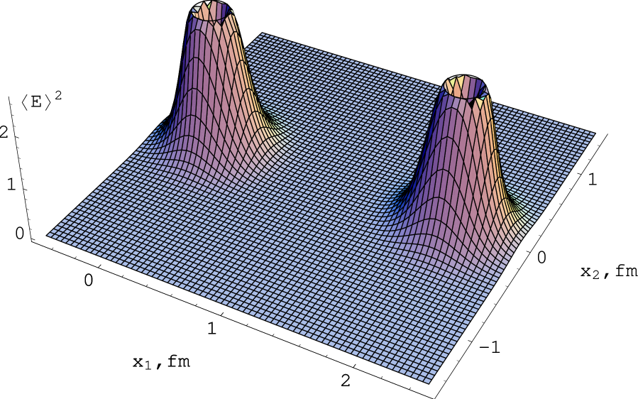
Figure 4: The total field distribution $\langle\mbox{\boldmath${\rm E}$}(x_{1},x_{2})\rangle^{2}$, measured in fm^-4, in case (a) at $T=1.070T_{c}$. $x_{1}$ and $x_{2}$ are measured in fm. $Q\bar{Q}$ separation $R=2$ fm.

In Fig. 4 we plot $\langle\mbox{\boldmath${\rm E}$}(x_{1},x_{2})\rangle^{2}$ distribution with parameters corresponding to the case $T=1.070T_{c}$ and $R=2$ fm. We observe two ”volcanoes” with quarks hidden in their bottoms. These two spherically symmetrical in coordinate space distributions are defined as

$$E(r)=Br^{2}K_{1}(r/\lambda),$$ (27)

where $r$ is a distance from quark or antiquark. The field at quark and antiquark positions is zero and linearly rises at small $r$. Maximal value of field is

$$E^{\max}=E(1.33\lambda)=0.63B\lambda^{2}.$$ (28)

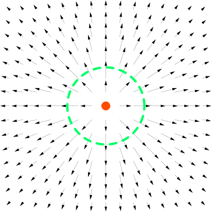
Figure 5: Vector distribution of $\langle\mbox{\boldmath${\rm E}$}(x_{1},x_{2})\rangle$ in case (a). $-0.5$ fm$<x_{1}<0.5$ fm,  $-0.5$ fm$<x_{2}<$0.5 fm. Quark position is marked with disk. Points of maximal value of field are marked with dashed circle of radius $1.33\lambda$.

In Fig. 5 the vector field distribution $\langle\mbox{\boldmath${\rm E}$}(x_{1},x_{2})\rangle$ is shown in the vicinity of the quark.

In the case (b) the transverse part of the field, $E_{2}$, remains the same (25). Let us calculate using (8) the longitudinal part of the field, $E_{1}$:

$$\langle E_{1}(x_{1},x_{2})\rangle_{Q\bar{Q}}^{(b)}=\int_{0}^{R}dx_{1}^{\prime}\int_{-\infty}^{\infty}dx_{4}^{\prime}\left(D(h^{2})+D_{1}(h^{2})+(h_{1}^{2}+h_{4}^{2})\frac{\partial D_{1}(h^{2})}{\partial h^{2}}\right)=$$

$$=\int_{x_{1}-R}^{x_{1}}dh_{1}\int_{-\infty}^{\infty}dh_{4}(-h_{2}^{2})\frac{\partial D_{1}}{\partial h^{2}}=\int_{x_{1}-R}^{x_{1}}dh_{1}\int_{0}^{\infty}dh_{4}\frac{h_{2}^{2}}{h\lambda}D_{1}=$$

$$=\frac{Bx_{2}^{2}}{\lambda}\int_{x_{1}-R}^{x_{1}}dh_{1}K_{0}(\sqrt{h_{1}^{2}+x_{2}^{2}}/\lambda).$$ (29)

In Fig. 6 we plot (29) for $T=1.070T_{c}$ and $R=2$ fm to observe the ”double quasistring”. The quasistring profile, $E_{1}(x_{2})\equiv\langle E_{1}(R/2,x_{2})\rangle_{Q\bar{Q}}^{(b)}$ at $R\to\infty$, is

$$E_{1}(x_{2})=\pi Bx_{2}^{2}\exp(-|x_{2}|/\lambda).$$ (30)

The field in the centre of quasistring is absent. The maximal value of the field is

$$E_{1}^{\max}=E_{1}(2\lambda)=1.7B\lambda^{2}.$$ (31)

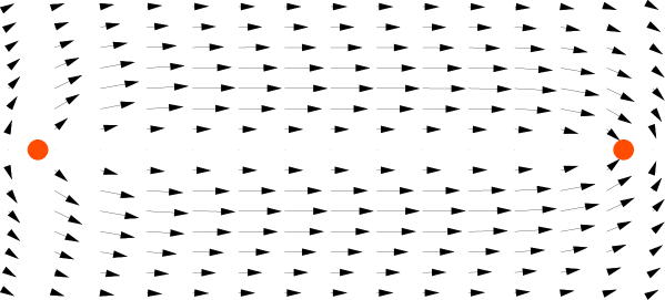
Figure 7: Vector distribution of $\langle\mbox{\boldmath${\rm E}$}(x_{1},x_{2})\rangle$ in case (b). Positions of $Q$ and $\bar{Q}$ are marked with disks. $-0.1$ fm$<x_{1}<$2.1 fm, $-0.5$ fm$<x_{2}<$0.5 fm.

In the coordinate space the quasistring resembles coaxial cable with empty core and tube shell. In Fig. 7 we plot $\langle\mbox{\boldmath${\rm E}$}(x_{1},x_{2})\rangle^{(b)}$ distribution around $Q$ and $\bar{Q}$.

6 Conclusions

Results of our paper based on the analysis of the lattice data on correlation functions at finite $T$ [1] give a full support of the dynamical picture of deconfinement, which was first suggested in [9].

Namely, confining and deconfining phases according to [9] differ first of all in the vacuum fields, i.e., in the value of the condensate and in the field correlators. It was argued in [9] that color magnetic correlators and their contribution to the condensate are kept intact across the temperature phase transition, while the confining electric part abruptly disappears above $T_{c}$. Both features are present in [1] and in the results of the present paper. Indeed, one can see from Tables 5,6, that the magnetic part of condensate is roughly constant around $T_{c}$. The role of magnetic field above $T_{c}$ was mentioned repeatedly in the literature, see recent lattice reviews [10], it reveals itself in particular in creating nonzero spatial string tension [9] and so-called screening hadronic masses – (see [11] and refs. therein).

The situation with electric fields is more subtle, as can be seen from our results. In [9] two possible situations have been considered when nonperturbative part of $D^{\mathrm{E}}$ vanishes or stays nonzero above $T_{c}$. From Figs. 4,6 one can clearly see the field distributions in cases of two possible solutions, (a) and (b), one with vanishing $D^{\mathrm{E,NP}}$, another with nonvanishing but oscillating $D^{\mathrm{E,NP}}$, both yielding zero string tension in the deconfinement region.

In the case (a) the electric contribution to condensate is determined by $D_{1}^{\mathrm{E,NP}}(0)$. While $D^{\mathrm{E,NP}}(x)$ vanishes identically, the $D_{1}^{\mathrm{E,NP}}$ correlator is different from zero above $T_{c}$ and its contribution to the condensate grows sharply with temperature. Hence the role of $D_{1}^{\mathrm{E,NP}}$ appears in creating the sharp rise of the ”nonideality” ($\varepsilon-3p$) just above $T_{c}$ (cf. Fig. 3). One special remark is due to the regime (b), where $D^{\mathrm{E,NP}}(x)$ is nonzero above $T_{c}$ but changing sign. This regime creates rather peculiar picture of fields — the ”quasistring” with the empty core and surrounding it tube shell at two correlation length distance from the quark axis (Fig. 6).

As the regime (a) seems to be more natural from physical point of view, one should study in more detail the consequences of the strongly increasing with $T$ $D_{1}^{\mathrm{E,NP}}(0)$ in the deconfining region.

The impossibility of resolving our present ambiguity (regimes (a) and (b)) calls for further numerical and analytical studies. It is necessary for understanding of the dynamics of the phase transition, where Polyakov loops and hence color-electric fields may play very important role.

The authors are grateful to A.Di Giacomo for useful remarks and suggestions; the partial support of grants 00-02-17836 and 00-15-96786 is gratefully acknowledged.

Table 1: Parameters of $D^{B}$.

T	0.956$T_{c}$	0.978$T_{c}$	1.011$T_{c}$
A, fm-4	188.9$\pm$2.4	154$\pm$2	183.1$\pm$3.0
$\lambda_{A}$, fm	0.1917$\pm$0.0007	0.2047$\pm$0.0008	0.1852$\pm$0.0008
B, fm-4	7.7$\pm$0.6	7.7$\pm$0.8	1.87$\pm$0.13
$\lambda_{B}$, fm	0.380$\pm$0.008	0.344$\pm$0.007	1.11$\pm$0.04
a	1.11$\pm$0.06	1.46$\pm$0.07	0.64$\pm$0.03
b	0.34$\pm$0.03	0.47$\pm$0.04	0.35$\pm$0.02
$\chi^{2}$/n	0.62	1.28	1.43
T	1.034$T_{c}$	1.070$T_{c}$	1.131$T_{c}$
A, fm-4	128.8$\pm$2.3	111.9$\pm$2.0	150.9$\pm$2.5
$\lambda_{A}$, fm	0.210$\pm$0.001	0.2191$\pm$0.0012	0.2009$\pm$0.0010
B, fm-4	2.92$\pm$0.23	3.54$\pm$0.29	3.07$\pm$0.23
$\lambda_{B}$, fm	0.69$\pm$0.02	0.631$\pm$0.017	0.774$\pm$0.024
a	0.92$\pm$0.04	1.039$\pm$0.043	0.885$\pm$0.031
b	0.47$\pm$0.03	0.525$\pm$0.032	0.506$\pm$0.023
$\chi^{2}$/n	0.53	1.18	0.58

Table 2: Parameters of $D^{E}$ below $T_{c}$.

T	0.956$T_{c}$	0.978$T_{c}$
A, fm-4	228$\pm$4	189.5$\pm$4.2
$\lambda_{A}$, fm	0.1823$\pm$0.0008	0.1812$\pm$0.0011
B, fm-4	10.8$\pm$0.5	14.3$\pm$0.6
$\lambda_{B}$, fm	0.435$\pm$0.011	0.411$\pm$0.006
a	3.1$\pm$0.4	0.99$\pm$0.08
b	0.9$\pm$0.2	0.71$\pm$0.18
$\chi^{2}$/n	0.39	1.7

Table 3: Parameters of $D^{E}$ at $T=1.011T_{c}$.

	(a): $D^{\mathrm{NP}}\equiv 0$	(b): $D_{||}^{\mathrm{NP}}\equiv 0$
B, fm-4	2.46$\pm$0.24	1.96$\pm$0.34
$\lambda_{B}$, fm	0.682$\pm$0.016	1.072$\pm$0.047
a	1.74$\pm$0.05	1.36$\pm$0.04
b	0.86$\pm$0.04	0.68$\pm$0.03
$\chi^{2}$/n	1.7	1.05

Table 4: Parameters of $D^{E}$ above $T_{c}$.

T	1.034$T_{c}$	1.070$T_{c}$	1.131$T_{c}$
B, fm-4	80$\pm$19	235$\pm$53	519$\pm$99
$\lambda_{B}$, fm	0.121$\pm$0.05	0.105$\pm$0.004	0.37$\pm$0.03
b	0.63$\pm$0.03	0.48$\pm$0.04	0.41$\pm$0.03
$\lambda_{b}$, fm	0.86$\pm$0.05	1.0$\pm$0.1	0.86$\pm$0.08
$\chi_{1}^{2}$	0.69	0.9	0.028
(a)  a	1.21$\pm$0.04	0.94$\pm$0.04	0.86$\pm$0.03
(a)  $\chi_{2}^{2}$	1.26	0.9	2.9
(b)  a	0.96$\pm$0.04	0.66$\pm$0.04	0.61$\pm$0.03
(b)  $\chi_{2}^{2}$	1.66	0.23	0.56

Table 5: Gluonic condensate below $T_{c}$.

T	0.956$T_{c}$	0.978$T_{c}$
$D^{\mathrm{B,NP}}(0)+D_{1}^{\mathrm{B,NP}}(0),$ fm-4	196.6$\pm$2.5	161.7$\pm$2.2
$D^{\mathrm{E,NP}}(0)+D_{1}^{\mathrm{E,NP}}(0),$ fm-4	238.8$\pm$4.0	203.8$\pm$4.2
$G_{2}(T)/G^{0}_{2}$	1.393$\pm$0.015	1.171$\pm$0.015

Table 6: Gluonic condensate above $T_{c}$.

	T	1.011$T_{c}$	1.034$T_{c}$	1.070$T_{c}$	1.131$T_{c}$
$D^{\mathrm{B,NP}}(0)+D_{1}^{\mathrm{B,NP}}(0),$ fm-4		185$\pm$3	131.7$\pm$2.3	115.4$\pm$2.0	154.0$\pm$2.5
$G_{2}(T)/G^{0}_{2}$	(a)	0.60$\pm$0.01	0.69$\pm$0.06	1.12$\pm$0.17	2.16$\pm$0.32
	(b)	0.59$\pm$0.01	0.422$\pm$0.007	0.370$\pm$0.006	0.493$\pm$0.008

Figure 1: Fitted functions $\ln D_{||}^{\mathrm{E}}(x)$ and $\ln D_{\bot}^{\mathrm{E}}(x)$ (shown by solid lines) at $T=0.978T_{c}$. $x$ is measured in fm. $D_{||}^{\mathrm{E}}$ and $D_{\bot}^{\mathrm{E}}$ are measured in fm^-4. Data are shown by points. Errors of data are comparable with size of the points. The separately shown error is two times enlarged by hand for the improvement of the fit.

Figure 2: Fitted function $\ln D_{\bot}^{\mathrm{E}}(x)$, shown by solid line in case (a) and dashed line in case (b) at $T=1.070T_{c}$. $x$ is measured in fm. $D_{\bot}^{\mathrm{E}}$ is measured in fm^-4. Data are shown by points joined by dashed lines. Errors of data are comparable with size of the points.

Figure 3: Gluon condensate dependence on $T/T_{c}$ near the deconfinement transition. Condensate is measured in its zero temperature value units. In the deconfinement region the magnetic part of condensate does not considerably change. Electric fields give rapidly rising contribution to condensate in case (a) and do no contribute to condensate in case (b).

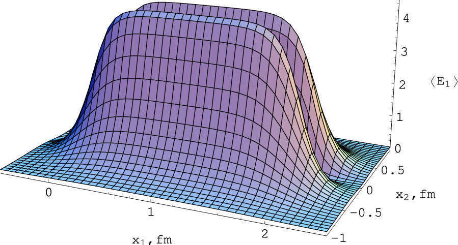
Figure 6: Distribution of $\langle E_{1}(x_{1},x_{2})\rangle$, measured in fm^-2, in case (b) at $T=1.070T_{c}$.

References

- [1] A.Di Giacomo, E.Meggiolaro, and H.Panagopoulos, Nucl.Phys. B 483 (1997) 371
- [2] H.G.Dosch, V.I.Shevchenko, and Yu.A.Simonov, hep-ph/0007223.
-
[3]
A.Di Giacomo, M.Maggiore, and S.Olejnik, Phys.Lett. B 236, 199
(1990); Nucl.Phys. B 347 441 (1990)
L.Del Debbio, A.Di Giacomo, and Yu.A.Simonov, Phys.Lett. B 332, 111 (1994). -
[4]
H.G.Dosch, Phys.Lett. B 190, 177 (1987);
H.G.Dosch and Yu.A.Simonov, Phys.Lett. B 205, 399 (1988);
Yu.A.Simonov, Nucl.Phys. B 307, 512 (1988). - [5] Yu.A.Simonov, Phys.Usp. 39, 313 (1996).
- [6] Review of Particle Physics, Eur.Phys.J. C 15 (2000).
- [7] A.Di Giacomo, E.Meggiolaro, and H.Panagopoulos, preprint IFUP-TH 12/96, hep-lat/9603017.
- [8] D.S.Kuzmenko and Yu.S.Simonov, Yad.Fiz. 64, 110 (2001), hep-ph/0010114.
-
[9]
Yu.A.Simonov, JETP Lett. 54, 256 (1991);
Yu.A.Simonov, JETP Lett. 55, 605 (1992);
Yu.A.Simonov, Yad.Fiz. 58, 357 (1995);
Yu.A.Simonov, Lectures at the E.Fermi International School, Varenna 1995, preprint ITEP-37-95. -
[10]
F.Karsch, Nucl.Phys.Proc.Suppl. 83, 14 (2000);
S.Ejiri, preprint UTCCP-P-95, hep-lat/0011006. - [11] E.L.Gubankova and Yu.A.Simonov, Phys.Lett. B 360, 93 (1995).
List of tables