Branching ratios and CP-violating asymmetries of $B_{s}\to h_{1}h_{2}$ decays in the general two-Higgs doublet models

Abstract

Based on the low-energy effective Hamiltonian with the generalized factorization, we calculate the new physics contributions to branching ratios and CP-violating asymmetries of the charmless hadronic decays $B_{s}\to h_{1}h_{2}$ in the standard model and the general two-Higgs doublet models (models I, II, and III). Within the considered paramter space, we find the following. (a) In models I and II, the new physics corrections are always small in size and will be masked by other larger known theoretical uncertainties. (b) In model III, the new physics corrections to the branching ratios of those QCD penguin-dominated decays $\overline{B}_{s}\to K^{0}\eta^{(^{\prime})},K^{+}K^{-*},etc.$, are large in size and insensitive to the variations of $M_{H^{+}}$ and $N_{c}^{{\rm eff}}$. For tree- or electroweak penguin-dominated decay modes, however, the new physics corrections are very small in size. (c) For $\overline{B}_{s}\to K^{+}K^{-*}$ and other seven decay modes, the branching ratios are at the level of $(1-3)\times 10^{-5}$ and will be measurable at the future hadron colliders with large $b$ production. (d) Among the studied thirty nine $B_{s}$ meson decay modes, seven of them can have a CP-violating asymmetry ${\cal A}_{CP}$ larger than $20\%$ in magnitude. The new physics corrections are small or moderate in magnitude. (e) Because of its large and $N_{c}^{{\rm eff}}$ stable branching ratio and CP violating asymmetry, the decay $\overline{B}_{s}\to K^{+}K^{-*}$ seems to be the “best” channel to find CP violation of $B_{s}$ system through studies of two-body charmless decays of $B_{s}$ meson.

PACS numbers: 13.25.Hw, 12.15.Ji, 12.38.Bx, 12.60.Fr

I Introduction

In B experiments, new physics beyond the standard model (SM) may manifest itself, for example, in following two ways[1, 2]: (a) decays which are expected to be rare in the SM are found to have large branching ratios; (b) CP-violating asymmetries which are expected to vanish or be very small in the SM are found to be significantly large or with a very different pattern with what predicted in the SM. These potential deviations may be induced by the virtual effects of new physics through loop diagrams.

The observation of many two-body charmless hadronic $B_{u,d}$ meson decays by CLEO, BaBar and Belle [3, 4, 5, 6, 7], the successful start of the asymmetric B factories at SLAC and KEK, and the expectation for large number of events of $B_{u,d}$ meson decays to be accumulated at B factories and other hadron colliders stimulated the intensive investigation for various B decay channels. The two-body charmless hadronic decays $B_{u,d}\to h_{1}h_{2}$ [ where $h_{1}$ and $h_{2}$ are the light pseudo-scalar (P) and/or vector(V) mesons ] have been studied, for example, in Refs. [8, 9, 10, 11, 12, 13].

It is well known that the low energy effective Hamiltonian is the basic tool to calculate the branching ratios and ${\cal A}_{CP}$ of B meson decays. The short-distance QCD corrected Lagrangian at NLO level is available now [14, 15], but we do not know how to calculate hadronic matrix element from first principles. One conventionally resort to the factorization approximation [16]. However, we also know that non-factorizable contribution really exists and can not be neglected numerically for most hadronic B decay channels. To remedy the naive factorization hypothesis, some authors [17, 10, 11] introduced a phenomenological parameter $N_{c}^{{\rm eff}}$ (i.e. the effective number of color) to model the non-factorizable contribution to hadronic matrix element, which is commonly called the generalized factorization. Very recently, Cheng et al. [18] studied and resolved the controversies on the gauge dependence and infrared singularity of the effective Wilson coefficients $C_{i}^{eff}$ [19] by using the perturbative QCD factorization theorem.

Unlike the $B_{u,d}$ meson, the heavier $B_{s}$ meson can not be produced in CESR, KEKB and PEP-II $e^{+}e^{-}$ colliders. Only upper limits on decay rates of several charmless hadronic $B_{s}$ decays are current available from LEP collaborations [20, 21], such as $B_{s}\to K^{+}K^{-}$, $K^{+}\pi^{-}$, $\pi^{0}\eta$ and $B_{s}\to\eta\eta$, while most of them are far beyond the theoretical predictions. However, it is expected that many $B_{s}$ decays can be seen at the future hadron colliders with large $b$ production. Recent theoretical studies and experimental measurements about the mixing of $B_{s}^{0}-\bar{B}^{0}_{s}$ can be found in Refs.[22, 23]. The early studies of two-dody charmless hadronic decays of $B_{s}$ meson can be found in Refs.[24, 25]. Based on the framework of generalized factorization, Tseng[26] analyzed the exclusive charmless $B_{s}$ decays involving $\eta^{(^{\prime})}$, while Chen, Cheng and Tseng [12] calculated the branching ratios of thirty nine charmless two-body decays of $B_{s}$ meson. It is found that the branching ratios of $\eta\eta^{(^{\prime})}$ and several other decay modes can be as large as $10^{-5}$ and measurable at future experiments.

In a recent work[27], we made a systematic study for the new physics contributions to the branching ratios of seventy six $B_{u,d}\to h_{1}h_{2}$ decay channels in the framework of the general two-Higgs-doublet models (2HDM’s). In this paper we extend the work to the case of $B_{s}$ meson. In additional to the branching ratios, we here also calculate the new physics contributions to the CP-violating asymmetries $A_{CP}$ of charmless hadronic decays $B_{s}\to h_{1}h_{2}$ induced by the new gluonic and eletroweak charged-Higgs penguin diagrams in the general 2HDM’s ( models I, II and III). Using the effective Hamiltonian with improved generalized factorization [18], we evaluate analytically all new strong and electroweak penguin diagrams induced by exchanges of charged Higgs bosons in the quark level processes $b\to qV^{*}$ with $q\in\{d,s\}$ and $V\in\{gluon,\;\gamma,Z\}$, and then combine the new physics contributions with their SM counterparts and finally calculate the branching ratios and CP-violating asymmetries for all thirty nine exclusive $B_{s}\to h_{1}h_{2}$ decay modes.

This paper is organized as follows. In Sec. II, we describe the basic structures of the 2HDM’s and examine the allowed parameter space of the general 2HDM’s from currently available data. In Sec. III, we evaluate analytically the new penguin diagrams and find the effective Wilson coefficients $C_{i}^{eff}$ with the inclusion of new physics contributions, and present the formulae needed to calculate the branching ratios ${\cal B}(B\to h_{1}h_{2})$. In Sec. IV and V, we calculate and show numerical results of branching ratios and CP-violating asymmetries for thirty nine $B_{s}$ decay modes, respectively. We focus on those decay modes with large branching ratios and large CP-violating asymmetries. The conclusions and discussions are included in the final section.

II The general 2HDM’s and experimental constraints

The simplest extension of the SM is the so-called two-Higgs-doublet models[28]. In such models, the tree level flavor changing neutral currents(FCNC’s) are absent if one introduces an discrete symmetry to constrain the 2HDM scalar potential and Yukawa Lagrangian. Lets consider a Yukawa Lagrangian of the form[29]

$${\cal L}_{Y} = \eta^{U}_{ij}\bar{Q}_{i,L}\tilde{\phi_{1}}U_{j,R}+\eta^{D}_{ij}\bar{Q}_{i,L}\phi_{1}D_{j,R}+\xi^{U}_{ij}\bar{Q}_{i,L}\tilde{\phi_{2}}U_{j,R}+\xi^{D}_{ij}\bar{Q}_{i,L}\phi_{2}D_{j,R}+h.c.,$$ (1)

where $\phi_{i}$ ($i=1,2$) are the two Higgs doublets of a two-Higgs-doublet model, $\tilde{\phi}_{1,2}=i\tau_{2}\phi^{*}_{1,2}$, $Q_{i,L}$ ($U_{j,R}$) with $i=(1,2,3)$ are the left-handed isodoublet quarks (right-handed up-type quarks), $D_{j,R}$ are the right-handed isosinglet down-type quarks, while $\eta^{U,D}_{i,j}$ and $\xi^{U,D}_{i,j}$ ($i,j=1,2,3$ are family index ) are generally the non-diagonal matrices of the Yukawa coupling. By imposing the discrete symmetry: $\phi_{1}\to-\phi_{1}$, $\phi_{2}\to\phi_{2}$, $D_{i}\to-D_{i}$, and $U_{i}\to\mp U_{i}$, one obtains the so called model I and model II.

During past years, models I and II have been studied extensively in literature and tested experimentally, and the model II has been very popular since it is the building block of the minimal supersymmetric standard model. In this paper, we focus on the third type of the two-Higgs-doublet model[30], usually known as the model III [29, 30]. In model III, no discrete symmetry is imposed and both up- and down-type quarks then may have diagonal and/or flavor changing couplings with $\phi_{1}$ and $\phi_{2}$. As described in [29], one can choose a suitable basis $(H^{0},H^{1},H^{2},H^{\pm})$ to express two Higgs doublets. The $H^{\pm}$ are the physical charged Higgs boson, $H^{0}$ and $h^{0}$ are the physical CP-even neutral Higgs boson and the $A^{0}$ is the physical CP-odd neutral Higgs boson. After the rotation of quark fields, the Yukawa Lagrangian of quarks are of the form [29],

$${\cal L}_{Y}^{III}=\eta^{U}_{ij}\bar{Q}_{i,L}\tilde{\phi_{1}}U_{j,R}+\eta^{D}_{ij}\bar{Q}_{i,L}\phi_{1}D_{j,R}+\hat{\xi}^{U}_{ij}\bar{Q}_{i,L}\tilde{\phi_{2}}U_{j,R}+\hat{\xi}^{D}_{ij}\bar{Q}_{i,L}\phi_{2}D_{j,R}+H.c.,$$ (2)

where $\eta^{U,D}_{ij}$ correspond to the diagonal mass matrices of up- and down-type quarks, while the neutral and charged flavor changing couplings will be [29]. We make the same ansatz on the $\xi^{U,D}_{ij}$ couplings as the Ref.[29]

$$\xi^{U,D}_{ij}=\frac{\sqrt{m_{i}m_{j}}}{v}\lambda_{ij},\ \ \hat{\xi}^{U,D}_{neutral}=\xi^{U,D},\ \ \hat{\xi}^{U}_{charged}=\xi^{U}V_{CKM},\ \ \hat{\xi}^{D}_{charged}=V_{CKM}\xi^{D},$$ (3)

where $V_{CKM}$ is the Cabibbo-Kobayashi-Maskawa mixing matrix [31], $i,j=(1,2,3)$ are the generation index. The coupling constants $\lambda_{ij}$ are free parameters to be determined by experiments, and they may also be complex.

In model II and setting $1\leq\tan{\beta}=v_{2}/v_{1}\leq 50$ favored by experimental measurements [20], the constraint on the mass of charged Higgs boson due to CLEO data of $b\to s\gamma$ is $M_{H^{+}}\geq 200$ GeV at the NLO level [32]. For model I, however, the limit can be much weaker due to the possible destructive interference with the SM amplitude. For model III, the situation is not as clear as model II because there are more free parameters here [29, 33]. In a recent paper [34], Chao et al. studied the decay $b\to s\gamma$ by assuming that only the couplings $\lambda_{tt}=|\lambda_{tt}|e^{i\theta_{t}}$ and $\lambda_{bb}=|\lambda_{bb}|e^{i\theta_{b}}$ are non-zero. They found that the constraint on $M_{H^{+}}$ imposed by the CLEO data of $b\to s\gamma$ can be greatly relaxed by considering the phase effects of $\lambda_{tt}$ and $\lambda_{bb}$. From the studies of Refs.[34, 35], we know that for model III the parameter space

$$\lambda_{ij}=0,\ \ for\ \ ij\neq tt,\ \ or\ \ bb,$$ (4)

$$|\lambda_{tt}|=0.3,\ \ |\lambda_{bb}|=35,\ \ \theta=(0^{\circ}-30^{\circ}),\ \ M_{H^{+}}=(200\pm 100){\rm GeV},$$ (5)

are allowed by the available data, where $\theta=\theta_{bb}-\theta_{tt}$.

From the CERN $e^{+}e^{-}$ collider (LEP) and the Fermilab Tevatron searches for charged Higgs bosons [36], the new combined constraint in the $(M_{H^{+}}\tan{\beta})$ plane has been given, for example, in Ref. [20]: the direct lower limit is $M_{H^{+}}>77$ GeV, while $0.5\leq\tan{\beta}\leq 60$ for a relatively light charged Higgs boson with $M_{H^{+}}\sim 100$ GeV. Combining the direct and indirect limits together, we here conservatively consider the range of $100{\rm GeV}\leq M_{H^{+}}\leq 300$ GeV, while take $M_{H^{+}}=200$ GeV as the typical value for models I, II, and III. For models I and II we consider the range of $1\leq\tan{\beta}\leq 50$, while take $\tan{\beta}=2$ as the typical value.

III Effective Hamiltonian in the SM and 2HDM’s

The standard theoretical frame to calculate the inclusive three-body decays $b\to s\bar{q}q$ is based on the effective Hamiltonian [15, 11, 13],

$${\cal H}_{eff}(\Delta B=1)=\frac{G_{F}}{\sqrt{2}}\left\{\sum_{j=1}^{2}C_{j}\left(V_{ub}V_{us}^{*}Q_{j}^{u}+V_{cb}V_{cs}^{*}Q_{j}^{c}\right)-V_{tb}V_{ts}^{*}\left[\sum_{j=3}^{10}C_{j}Q_{j}+C_{g}Q_{g}\right]\right\}$$ (6)

Here the first ten operators $Q_{1}-Q_{10}$ can be found for example in Refs.[11, 13, 27], while the chromo-magnetic operator reads:

$$Q_{g} = \frac{g_{s}}{8\pi^{2}}m_{b}\bar{s}_{\alpha}\sigma^{\mu\nu}(1+\gamma_{5})T^{a}_{\alpha\beta}b_{\beta}G^{a}_{\mu\nu}$$ (7)

where $\alpha$ and $\beta$ are the $SU(3)$ color indices, $T^{a}_{\alpha\beta}$ ( $a=1,...,8$) are the Gell-Mann matrices. Following Ref.[12], we do not consider the effect of the weak annihilation and exchange diagrams.

The coefficients $C_{i}$ in Eq.(6) are the well-known Wilson coefficient. Within the SM and at scale $M_{W}$, the Wilson coefficients $C_{1}(M_{W}),\cdots,C_{10}(M_{W})$ and $C_{g}(M_{W})$ have been given for example in Refs.[14, 15]. By using QCD renormalization group equations, it is straightforward to run Wilson coefficients $C_{i}(M_{W})$ from the scale $\mu=0(M_{W})$ down to the lower scale $\mu=O(m_{b})$. Working consistently to the NLO precision, the Wilson coefficients $C_{i}$ for $i=1,\ldots,10$ are needed in NLO precision, while it is sufficient to use the leading logarithmic value for $C_{g}$.

A New strong and electroweak penguins

For the charmless hadronic decays of B meson under consideration, the new physics will manifest itself by modifying the corresponding Inami-Lim functions $C_{0}(x),D_{0}(x),E_{0}(x)$ and $E^{\prime}_{0}(x)$ which determine the coefficients $C_{3}(M_{W}),\ldots,C_{10}(M_{W})$ and $C_{g}(M_{W})$. These modifications, in turn, will change the SM predictions of the branching ratios and CP-violating asymmetries for decays $B_{s}\to h_{1}h_{2}$ under study.

The new strong and electroweak penguin diagrams can be obtained from the corresponding penguin diagrams in the SM by replacing the internal $W^{\pm}$ lines with the charged-Higgs $H^{+}$ lines. In Ref.[27], we calculated analytically the new $Z^{0}$-, $\gamma$- and gluon-penguin diagrams induced by the exchanges of charged-Higgs boson $H^{+}$, and found the new $C_{0},D_{0},E_{0}$, and $E^{\prime}_{0}$ functions which describe the new physics contributions to the Wilson coefficients through the new penguin diagrams,

$$C_{0}^{III} = \frac{-x_{t}}{16}\left[\frac{y_{t}}{1-y_{t}}+\frac{y_{t}}{(1-y_{t})^{2}}\ln[y_{t}]\right]\cdot|\lambda_{tt}|^{2}$$ (8)

$$D_{0}^{III} = -\frac{1}{3}H(y_{t})|\lambda_{tt}|^{2}$$ (9)

$$E_{0}^{III} = -\frac{1}{2}I(y_{t})|\lambda_{tt}|^{2},$$ (10)

$${E^{\prime}_{0}}^{III} = \frac{1}{6}J(y_{t})|\lambda_{tt}|^{2}-K(y_{t})|\lambda_{tt}\lambda_{bb}|e^{i\theta},$$ (11)

with

$$H(y) = \frac{38y-79y^{2}+47y^{3}}{72(1-y)^{3}}+\frac{4y-6y^{2}+3y^{4}}{12(1-y)^{4}}\ln[y]$$ (12)

$$I(y) = \frac{16y-29y^{2}+7y^{3}}{36(1-y)^{3}}+\frac{2y-3y^{2}}{6(1-y)^{4}}\log[y],$$ (13)

$$J(y) = \frac{2y+5y^{2}-y^{3}}{4(1-y)^{3}}+\frac{3y^{2}}{2(1-y)^{4}}\log[y],$$ (14)

$$K(y) = \frac{-3y+y^{2}}{4(1-y)^{2}}-\frac{y}{2(1-y)^{3}}\log[y].$$ (15)

where $x_{t}=m_{t}^{2}/M_{W}^{2}$, $y_{t}=m_{t}^{2}/M_{H^{+}}^{2}$, and the small terms proportional to $m_{b}^{2}/m_{t}^{2}$ have been neglected. In models I and II, one can find the corresponding functions $C_{0}$, $D_{0}$,$E_{0}$ and $E^{\prime}_{0}$ by evaluating the new strong and electroweak penguins in the same way as that in model III:

$$C_{0}^{I} = C_{0}^{II}=\frac{-x_{t}}{8\tan^{2}{\beta}}\left[\frac{y_{t}}{1-y_{t}}+\frac{y_{t}}{(1-y_{t})^{2}}\ln[y_{t}]\right],$$ (16)

$$D_{0}^{I} = D_{0}^{II}=-\frac{2}{3\tan^{2}{\beta}}H(y_{t}),$$ (17)

$$E_{0}^{I} = E_{0}^{II}-\frac{1}{\tan^{2}{\beta}}I(y_{t}),$$ (18)

$${E^{\prime}_{0}}^{I} = \frac{1}{3\tan^{2}{\beta}}\left[J(y_{t})-6K(y_{t})\right],$$ (19)

$${E^{\prime}_{0}}^{II} = \frac{1}{3\tan^{2}{\beta}}J(y_{t})+2K(y_{t}),$$ (20)

where $y_{t}=m_{t}^{2}/M_{H^{+}}^{2}$, $\tan{\beta}=v_{2}/v_{1}$ where $v_{1}$ and $v_{2}$ are the vacuum expectation values of the Higgs doublet $\phi_{1}$ and $\phi_{2}$ as defined before.

Combining the SM part and the new physics part together, the NLO Wilson coefficients $C_{i}(M_{W})$ and $C_{g}(M_{W})$ can be written as

$$C_{1}(M_{W}) = 1-\frac{11}{6}\;\frac{\alpha_{s}(M_{W})}{4\pi}-\frac{35}{18}\;\frac{\alpha_{em}}{4\pi}\,,$$ (21)

$$C_{2}(M_{W}) = \frac{11}{2}\;\frac{\alpha_{s}(M_{W})}{4\pi}\,,$$ (22)

$$C_{3}(M_{W}) = -\frac{\alpha_{s}(M_{W})}{24\pi}\left[E_{0}(x_{t})+E_{0}^{NP}-\frac{2}{3}\right]$$ (24)

$$+\frac{\alpha_{em}}{6\pi}\frac{1}{\sin^{2}\theta_{W}}\left[2B_{0}(x_{t})+C_{0}(x_{t})+C_{0}^{NP}\right]\,,$$

$$C_{4}(M_{W}) = \frac{\alpha_{s}(M_{W})}{8\pi}\left[E_{0}(x_{t})+E_{0}^{NP}-\frac{2}{3}\right]\,,$$ (25)

$$C_{5}(M_{W}) = -\frac{\alpha_{s}(M_{W})}{24\pi}\left[E_{0}(x_{t})+E_{0}^{NP}-\frac{2}{3}\right]\,,$$ (26)

$$C_{6}(M_{W}) = \frac{\alpha_{s}(M_{W})}{8\pi}\left[E_{0}(x_{t})+E_{0}^{NP}-\frac{2}{3}\right]\,,$$ (27)

$$C_{7}(M_{W}) = \frac{\alpha_{em}}{6\pi}\left[4C_{0}(x_{t})+4C_{0}^{NP}+D_{0}(x_{t})+D_{0}^{NP}-\frac{4}{9}\right]\,,$$ (28)

$$C_{8}(M_{W}) = C_{10}(M_{W})=0\,,$$ (29)

$$C_{9}(M_{W}) = \frac{\alpha_{em}}{6\pi}\left\{4C_{0}(x_{t})+4C_{0}^{NP}+D_{0}(x_{t})+D_{0}^{NP}-\frac{4}{9}\right.$$ (31)

$$\left.+\frac{1}{\sin^{2}\theta_{W}}\left[10B_{0}(x_{t})-4C_{0}(x_{t})+4C_{0}^{NP}\right]\right\}\,,$$

$$C_{g}(M_{W}) = -\frac{1}{2}\left(E^{\prime}_{0}(x_{t})+{E^{\prime}}_{0}^{NP}\right)\,,$$ (32)

where $x_{t}=m_{t}^{2}/M_{W}^{2}$, the functions $B_{0}(x)$, $C_{0}(x)$, $D_{0}(x)$, $E_{0}(x)$ and $E^{\prime}_{0}$ are the familiar Inami-Lim functions [37] in the SM and can be found easily, for example, in Refs. [14, 38].

Since the heavy new particles appeared in the 2HDM’s have been integrated out at the scale $M_{W}$, the QCD running of the Wilson coefficients $C_{i}(M_{W})$ down to the scale $\mu=O(m_{b})$ after including the new physics contributions will be the same as in the SM:

$${\bf C}(\mu) = U(\mu,M_{W}){\bf C}(M_{W}),$$ (33)

$$C_{g}(\mu) = \eta^{14/23}C_{g}(M_{W})+\sum_{i=1}^{8}\bar{h}_{i}\eta^{a_{i}},$$ (34)

where ${\bf C}(M_{W})=(C_{1}(M_{W}),\ldots,C_{10}(M_{W}))^{T}$, $U(\mu,M_{W})$ is the five-flavor $10\times 10$ evolution matrix at NLO level as defined in Ref.[14], $\eta=\alpha_{s}(M_{W})/\alpha_{s}(\mu)$, and the constants $\bar{h}_{i}$ and $a_{i}$ can also be found in Ref.[14].

In the NDR scheme and for $SU(3)_{C}$, the effective Wilson coefficients can be written as [13]

$$C_{i}^{eff} = \left[1+\frac{\alpha_{s}}{4\pi}\,\left(\hat{r}_{V}^{T}+\gamma_{V}^{T}\log\frac{m_{b}}{\mu}\right)\right]_{ij}\,C_{j}+\frac{\alpha_{s}}{24\pi}\,A_{i}^{\prime}\left(C_{t}+C_{p}+C_{g}\right)+\frac{\alpha_{ew}}{8\pi}\,B_{i}^{\prime}C_{e}~{},$$ (35)

where $A_{i}^{\prime}=(0,0,-1,3,-1,3,0,0,0,0)^{T}$, $B_{i}^{\prime}=(0,0,0,0,0,0,1,0,1,0)^{T}$, the matrices $\hat{r}_{V}$ and $\gamma_{V}$ contain the process-independent contributions from the vertex diagrams. The matrix $\gamma_{V}$ and $\hat{r}_{V}$ have been given explicitly, for example, in Eq.(2.17) and (2.18) of Ref.[13]. Note that the correct value of the element $(\hat{r}_{NDR})_{66}$ and $(\hat{r}_{NDR})_{88}$ should be 17 instead of 1 as pointed in Ref.[39].

The function $C_{t}$, $C_{p}$, and $C_{g}$ describe the contributions arising from the penguin diagrams of the current-current $Q_{1,2}$ and the QCD operators $Q_{3}$-$Q_{6}$, and the tree-level diagram of the magnetic dipole operator $Q_{8G}$, respectively. We here also follow the procedure of Ref.[10] to include the contribution of magnetic gluon penguin. The functions $C_{t}$, $C_{p}$, and $C_{g}$ are given in the NDR scheme by [11, 13]

$$C_{t} = \left[\frac{2}{3}+{\lambda_{u}\over\lambda_{t}}G(m_{u})+{\lambda_{c}\over\lambda_{t}}G(m_{c})\right]C_{1},$$ (36)

$$C_{p} = \left[\frac{4}{3}-G(m_{q})-G(m_{b})\right]C_{3}+\left[\frac{10}{3}-\sum_{i=u,d,s,c,b}G(m_{i})\right](C_{4}+C_{6}),$$ (37)

$$C_{e} = {8\over 9}\left[\frac{2}{3}+{\lambda_{u}\over\lambda_{t}}G(m_{u})+{\lambda_{c}\over\lambda_{t}}G(m_{c})\right](C_{1}+3C_{2}),$$ (38)

$$C_{g} = -{2m_{b}\over\sqrt{<k^{2}>}}C^{\rm eff}_{g},$$ (39)

with $\lambda_{q^{\prime}}\equiv V_{q^{\prime}b}V_{q^{\prime}q}^{*}$, and $C_{g}^{eff}=C_{g}(\mu)+C_{5}$. The function $G(m)$ can be found, for example, in Refs. [13, 27]. For the two-body exclusive B meson decays any information on $k^{2}$ is lost in the factorization assumption, one usually use the ”physical” range for $k^{2}$ [11, 12, 13]: $\frac{m_{b}^{2}}{4}\stackrel{{\scriptstyle<}}{{\sim}}k^{2}\stackrel{{\scriptstyle<}}{{\sim}}\frac{m_{b}^{2}}{2}$. Following Refs.[11, 12, 13] we take $k^{2}=m_{b}^{2}/2$ in the numerical calculation.

B Decay amplitudes in the BSW model

Following Ref.[12], the possible effects of final state interaction (FSI) and the contributions from annihilation channels will be neglected although they may play a significant rule for some decay modes. The new physics effects on the B decays under study will be included by using the modified effective coefficients $a_{i}$ ($i=3,\dots,10$) as given in the second entries of Table I and Table II for the model III. The effective coefficients $a_{i}$ in models I and II are not shown explicitly in Table I and Table II. In the numerical calculations the input parameters as given in Appendix and Eq.(5) will be used implicitly.

With the factorization ansatz [16], the three-hadron matrix elements or the decay amplitude $<XY|H_{eff}|B_{s}>$ can be factorized into a sum of products of two current matrix elements $<X|J_{1}^{\mu}|0>$ and $<Y|J_{2\mu}|B_{s}>$ ( or $<Y|J_{1}^{\mu}|0>$ and $<X|J_{2\mu}|B_{s}>$). The explicit expressions of matrix elements can be found, for example, in Refs.[16, 40].

In the B rest frame, the branching ratios of two-body B meson decays can be written as

$${\cal B}(B_{s}\to XY)=\tau_{B_{s}}\,\frac{|p|}{8\pi M_{B_{s}}^{2}}|M(B_{s}\to XY)|^{2}$$ (40)

for $B_{s}\to PP$ decays, and

$${\cal B}(B_{s}\to XY)=\tau_{B_{s}}\,\frac{|p|^{3}}{8\pi M_{V}^{2}}|M(B_{s}\to XY)/(\epsilon\cdot p_{B})|^{2}$$ (41)

for $B_{s}\to PV$ decays. Here $\tau(B_{s}^{0})=1.493ps$[20], $p_{B}$ is the four-momentum of the B meson, $M_{V}$ and $\epsilon$ is the mass and polarization vector of the produced light vector meson respectively, and $|p|$ is the magnitude of momentum of particle X and Y in the B rest frame,

$$|p|=\frac{1}{2M_{B}}\sqrt{[M_{B}^{2}-(M_{X}+M_{Y})^{2}][M_{B}^{2}-(M_{X}-M_{Y})^{2}]}$$ (42)

For $B_{s}\to VV$ decays, the situation is more involved. One needs to evaluate the helicity matrix element $H_{\lambda}=<V_{1}(\lambda)V_{2}(\lambda)|H_{eff}|B)>$ with $\lambda=0,\pm 1$. The branching ratio of the decay $B\to V_{1}V_{2}$ is given in terms of $H_{\lambda}$ by

$${\cal B}(B_{s}\to V_{1}V_{2}) = \tau_{B_{s}}\,\frac{|p|}{8\pi M_{B}^{2}}\left(|H_{0}|^{2}+|H_{+1}|^{2}+|H_{-1}|^{2}\right)$$ (43)

where $|p|$ has been given in Eq.(42). The three independent helicity amplitudes $H_{0}$, $H_{+1}$ and $H_{-1}$ can be expressed by three invariant amplitudes $a,b,c$ defined by the decomposition

$$H_{\lambda} = i\epsilon^{\mu}(\lambda)\eta^{\nu}(\lambda)\left[ag_{\mu\nu}+\frac{b}{M_{1}M_{2}}p_{\mu}p_{\nu}+\frac{ic}{M_{1}M_{2}}\epsilon_{\mu\nu\alpha\beta}p_{1}^{\alpha}p^{\beta}\right]$$ (44)

where $p_{1,2}$ and $M_{1,2}$ are the four momentum and masses of $V_{1,2}$, respectively. $p=p_{1}+p_{2}$ is the four-momentum of B meson, and

$$H_{\pm 1} = a\pm c\sqrt{x^{2}-1},~{}~{}~{}~{}H_{0}=-ax-b\left(x^{2}-1\right)$$ (45)

$$x = \frac{M_{B}^{2}-M_{1}^{2}-M_{2}^{2}}{2M_{1}M_{2}}$$ (46)

For individual decay mode, the coefficients $a,b$ and $c$ can be determined by comparing the helicity amplitude $H_{\lambda}=<V_{1}(\lambda)V_{2}(\lambda)|H_{eff}|B_{s}>$ with the expression (44).

In the generalized factorization approach, the effective Wilson coefficients $C_{i}^{eff}$ will appear in the decay amplitudes in the combinations:

$$a_{2i-1}\equiv C_{2i-1}^{{\rm eff}}+\frac{{C}_{2i}^{{\rm eff}}}{N_{c}^{{\rm eff}}},\ \ a_{2i}\equiv C_{2i}^{{\rm eff}}+\frac{{C}_{2i-1}^{{\rm eff}}}{N_{c}^{{\rm eff}}},\ \ \ (i=1,\ldots,5)$$ (47)

where the effective number of colors $N_{c}^{{\rm eff}}$ is treated as a free parameter varying in the range of $2\leq N_{c}^{{\rm eff}}\leq\infty$, in order to model the non-factorizable contribution to the hadronic matrix elements. Although $N_{c}^{{\rm eff}}$ can in principle vary from channel to channel, but in the energetic two-body hadronic B meson decays, it is expected to be process insensitive as supported by the data [12]. As argued in ref.[17], $N_{c}^{{\rm eff}}(LL)$ induced by the $(V-A)(V-A)$ operators can be rather different from $N_{c}^{{\rm eff}}(LR)$ generated by $(V-A)(V+A)$ operators. Since we here focus on the calculation of new physics effects on the studied B meson decays induced by the new penguin diagrams in the two-Higgs doublet models, we will simply assume that $N_{c}^{{\rm eff}}(LL)\equiv N_{c}^{{\rm eff}}(LR)=N_{c}^{{\rm eff}}$ and consider the variation of $N_{c}^{{\rm eff}}$ in the range of $2\leq N_{c}^{{\rm eff}}\leq\infty$. For more details about the cases of $N_{c}^{{\rm eff}}(LL)\neq N_{c}^{{\rm eff}}(LR)$, one can see for example Ref.[12]. We here will not consider the possible effects of final state interaction (FSI) and the contributions from annihilation channels although they may play a significant rule for some decay modes.

Using the input parameters as given in Appendix, and assuming $k^{2}=m_{b}^{2}/2$, $M_{H^{+}}=200$ GeV, the theoretical predictions of effective coefficients $a_{i}$ are calculated and displayed in Table I and Table II for the transitions $b\to d$ ( $\bar{b}\to\bar{d}$ ) and $b\to s$ ($\bar{b}\to\bar{s}$), respectively. For coefficients $a_{3},\ldots,a_{10}$, the first and second entries in tables (I,II) refer to the values of $a_{i}$ in the SM and model III, respectively.

Compared with Ref.[12], the effective coefficients $a_{i}$ given here have two new features:

• The effective Wilson coefficients $C_{i}^{eff}$ here are not only renormalization scale- and scheme-independent, but also gauge invariant and infrared safe.

• The contribution due to the chromo-magnetic dipole operator $Q_{g}$ has been included here through the function $C_{g}$ as given in Eq.(39). For the penguin dominated decay channels, operator $C_{g}$ will play an important role.

• The coefficient $a_{1}$ and $a_{2}$ remain unchanged in 2HDM’s since the new physics considered here does not contribute through tree diagrams.

• The new physics contributions are significant to coefficient $a_{4}$ and $a_{6}$, but negligibly small to coefficients $a_{3,5}$ and $a_{7-10}$.

All branching ratios here are the averages of the branching ratios of $B$ and anti-$B$ decays. The ratio $\delta{\cal B}$ describes the new physics correction on the decay ratio and is defined as

$$\delta{\cal B}(B_{s}\to XY)=\frac{{\cal B}(B_{s}\to XY)^{NP}-{\cal B}(B_{s}\to XY)^{SM}}{{\cal B}(B_{s}\to XY)^{SM}}$$ (48)

IV Branching ratios of $B_{s}$ meson decays

Using the formulas and input parameters as given in last section and in Appendix, it is straightforward to find the branching ratios for the thirty nine $B_{s}\to PP,PV,VV$ decay channels. In the numerical calculations, we use the decay amplitudes as given in Appendix A, B and C of Ref.[12] directly without further discussions about details.

Following Ref.[16, 12], the hadronic charmless $B$ meson decays can be classified into six classes: the first and last three classes correspond to the tree-dominated and penguin-dominated amplitudes, respectively.

• Class-I and Class-II decays are dominated by the external and internal W-emission tree-diagrams, respectively. Examples are $\overline{B}_{s}\to K^{+}\pi^{-},K^{0}\pi^{0},\cdots.$

• Class-III: the decays involving both external and internal W-emissions. But this class does not exist for the $B_{s}$ decays.

• Class-IV and Class-V decay modes are governed by effective coefficients $a_{4,6,8,10}$ and $a_{3,5,7,9}$, respectively. Examples are $\overline{B}_{s}\to K^{+}K^{-},\pi\eta^{(^{\prime})},\cdots.$

• Class-VI decays involve the interference of class-IV and class-V decays.

In tables III-VI, we present the numerical results of the branching ratios for the thirty nine $B_{s}\to PP,PV,VV$ decays in the framework of the SM and models I, II and III. Theoretical predictions are made by using the central values of input parameters as given in Eq.(5) and Appendix, and assuming $A=0.804$, $\lambda=0.22$, $\rho=0.16$, $\eta=0.34$, $M_{H^{+}}=200$GeV, $\theta=0^{\circ},30^{\circ}$, $\tan{\beta}=2$ and $N_{c}^{{\rm eff}}=2,3,\infty$ in the generalized factorization approach. The $k^{2}$-dependence of the branching ratios is small in the range of $k^{2}=m_{b}^{2}/2\pm 2\;GeV^{2}$ and hence the numerical results are given by fixing $k^{2}=m_{b}^{2}/2$.

The SM predictions for all $B_{s}$ decay modes as listed in tables III and IV are agree well with those given in Ref.[12]. The effect of changing $\hat{r}_{V}$ and including the new contribution from the chromo-magnetic operator $Q_{g}$ in the SM is not significant.

For decay modes involving $B_{s}\to K^{*}$ or $B_{s}\to\phi$ transitions, we use two different set of form factors: the Bauer, Stech, and Wirbel (BSW) form factor[16] and the light-cone sum rule(LCSR) form factor as given explicitly in Appendix. For decay modes $B_{s}\to\pi^{0}\phi,\phi\eta^{\prime},\rho^{0}\phi,\omega\phi$ and $B_{s}\to\phi\phi$, the variation of the branching ratios induced by using different set of form factors is about a factor of 2, but small or moderate for all other decay modes.

From numerical results, we see the following general features of new physics corrections:

• In model III, the new physics corrections to QCD-penguin dominated decay modes, such as $B_{s}\to K^{0}\eta^{(^{\prime})},\eta^{(^{\prime})}\eta^{(^{\prime})},K^{0}\bar{K}^{0},etc.$, are large in size and insensitive to the variations of the mass $M_{H^{+}}$ and $N_{c}^{{\rm eff}}$: from $~{}30\%$ to $~{}130\%$ $w.r.t$ the SM predictions for both cases of $\theta=0^{\circ},30^{\circ}$. For tree-dominated or electroweak penguin dominated decay modes, however, the new physics corrections are very small in size: $\delta{\cal B}\leq 5\%$.

• In models I and II, the new physics corrections to all $B_{s}\to h_{1}h_{2}$ decay modes are always small in size within the considered parameter space: less than $10\%$ and $20\%$ in model I and II respectively, as shown in tables V and VI. So small corrections will be masked by other larger known theoretical uncertainties. Variation of $\tan{\beta}$ in the range of $2\leq\tan{\beta}\leq 50$ can not change this feature.

• In model III, the new gluonic penguins will contribute effectively through the mixing of chromo-magnetic operator $Q_{g}$ with QCD penguin operators $Q_{3}-Q_{6}$, as shown in Eq.(35). The $C_{g}^{eff}$ will strongly dominate the new physics contributions to $B_{s}$ meson decays. The branching ratios for all thirty nine decay modes have a very weak dependence on $\theta$ in the range of $0^{\circ}\leq\theta\leq 30^{\circ}$.

As pointed in Refs.[12, 41], the decays

$$\overline{B}_{s}\to\eta\pi,\eta^{\prime}\pi,\eta\rho,\eta^{\prime}\rho,\phi\pi,\phi\rho$$ (49)

do not receive any QCD penguin contributions, and are predominately governed by $a_{9}$ and hence $N_{c}^{{\rm eff}}$ insensitive. In 2HDM’s, this remain to be true because the new physics corrections to coefficients $a_{7-10}$ are negligibly small as shown in tables I and II, and therefore, the new physics contributions to these decay modes are also very small: $\leq 2\%$. As suggested in Ref.[12], a measurement of these six decay modes can be utilized to fix the parameter $a_{9}$. It is clear that the inclusion of new physics contributions in the 2HDM’s does not change this picture.

For the decays

$$\overline{B}_{s}\to\omega\eta,\omega\eta^{\prime},\phi\eta^{(^{\prime})},K\phi,K^{*}\phi,\phi\pi,$$ (50)

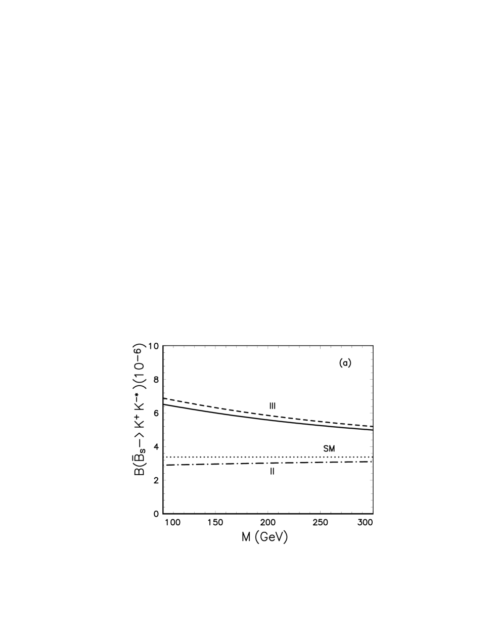
the SM electroweak penguin corrections are in general as important as QCD penguin effects, and very sensitive on $N_{c}^{{\rm eff}}$. The new physics corrections to these decay modes in the model III also have a strong dependence on the variation of $N_{c}^{{\rm eff}}$: $\delta{\cal B}=-20\%-110\%$ for $2\leq N_{c}^{{\rm eff}}\leq\infty$. As illustrated in Fig. 1, for example, the branching ratio of $B_{s}\to\phi\eta$ decay has a moderate $M_{H^{+}}$-dependence, but a strong $N_{c}^{{\rm eff}}$ dependence. For Fig. 1(a) and 1(b), we set $N_{c}^{{\rm eff}}=3$ and $M_{H^{+}}=200$ GeV, respectively. The four curves correspond to the theoretical predictions in the SM (dotted curve), model II (dot-dashed curve), model III with $\theta=0^{\circ}$ (solid curve) and $\theta=30^{\circ}$ (short-dashed curve), respectively.

Among the thirty nine charmless two-body hadronic $B_{s}$ decays, we find that only 7 (8) of them have branching ratios at the level of $10^{-5}$ in the SM (model III):

$$\overline{B}_{s}\to K^{+}K^{-},K^{0}\overline{K}^{0},\eta\eta,\eta^{\prime}\eta^{(^{\prime})},K^{+}\rho,K^{+*}\rho^{-},\phi\phi.$$ (51)

Among these eight decay modes, the new physics correction to the Class-I decay mode $\overline{B}_{s}\to K^{+}\rho^{-}$ and $K^{+*}\rho^{-}$ are very small, from $-2\%$to $1\%$. For remaining six decay modes, the new physics enhancement are significant: from $\sim 50\%$ to $\sim 130\%$ and insensitive to the variation of $N_{c}^{{\rm eff}}$. These decay modes will be measurable at the future hadron colliders with large $b$ production [12]. In Figs. 2 and 3, we plot the mass and $N_{c}^{{\rm eff}}$ dependence of the branching ratios of $\overline{B}_{s}\to K^{+}K^{-}$ and $\eta\eta^{\prime}$ decay modes.

After inclusion of new physics contributions in the models I, II and III, the patterns observed in Ref.[12] remain unchanged,

$$\Gamma(\overline{B}_{s}\to K^{+}K^{-})>\Gamma(\overline{B}_{s}\to K^{+}K^{*-}){\ \lower-1.2pt\vbox{\hbox{\hbox to0.0pt{$>$\hss}\lower 5.0pt\vbox{\hbox{$\sim$}}}}\ }\Gamma(\overline{B}_{s}\to K^{*+}K^{*-})>\Gamma(\overline{B}_{s}\to K^{+*}K^{-}),$$ (52)

$$\Gamma(\overline{B}_{s}\to K^{0}\overline{K}^{0})>\Gamma(\overline{B}_{s}\to K^{0}\overline{K}^{*0}){\ \lower-1.2pt\vbox{\hbox{\hbox to0.0pt{$>$\hss}\lower 5.0pt\vbox{\hbox{$\sim$}}}}\ }\Gamma(\overline{B}_{s}\to K^{*0}\overline{K}^{*0})>\Gamma(\overline{B}_{s}\to K^{*0}\overline{K}^{0}).$$ (53)

Recently, large decay rates for $B_{u}^{+}\to K^{+}\eta^{\prime}$ and $B_{d}\to K^{0}\eta^{\prime}$ decays have been reported by CLEO and BaBar collaborations [4, 5]. The CLEO measurement of $B_{d}^{0}\to K^{0}\eta^{\prime}$ decay is ${\cal B}(B_{d}^{0}\to K^{0}\eta^{\prime})=(89^{+18}_{-16}\pm 9)\times 10^{-6}$, which is larger than the branching ratios of $B\to K\pi$ decays by a factor of 3 to 5. For $B_{s}$ decays, the decay modes $\overline{B}_{s}\to\eta\eta^{\prime}$ and $\overline{B}_{s}\eta^{\prime}\eta^{\prime}$ are the analogue of $B_{d}\to K^{0}\eta^{\prime}$ decay, and are expected to have large branching ratios. From Table III, one can see that the SM predictions of the branching ratios ${\cal B}(B_{s}\to\eta\eta^{\prime})$ and ${\cal B}(B_{s}\to\eta^{\prime}\eta^{\prime})$ are indeed large, but in comparable size with other six decay modes listed in Eq.(51). The new physics enhancement to these two decay modes are significant in size, $\sim 70\%$ in model III, as illustrated in Fig. 3. After inclusion of new physics contributions, we find numerically that

$${\cal B}(\overline{B}_{s}\to\eta\eta^{\prime})\approx(23-33)\times 10^{-6}~{},$$ (54)

$${\cal B}(\overline{B}_{s}\to\eta^{\prime}\eta^{\prime})\approx(12-16)\times 10^{-6}~{}.$$ (55)

These theoretical predictions will be tested by the future experimental measurements.

For decays $\overline{B}\to K^{+}K^{-*}$ and $\overline{B}\to K^{+*}K^{-*}$, they have relatively large decay rates and weak $M_{H^{+}}$ and $N_{c}^{{\rm eff}}$ dependence. In Figs. 4 and 5, we plot the mass and $N_{c}^{{\rm eff}}$ dependence of the branching ratios ${\cal B}(\overline{B}_{s}\to K^{+}K^{-*})$ and ${\cal B}(K^{+*}K^{-*})$. It is easy to see that the new physics contributions in the model III to these two Class-IV decays are significant ( $\sim 70\%$ ) in size and insensitive to the variations of $M_{H^{+}}$ and $N_{c}^{{\rm eff}}$.

V CP-violating asymmetries of $B_{s}$ meson decays

In Ref.[25], Du et al. studied the branching ratios and CP-violating asymmetries for decay modes $B_{s}\to K^{-}\pi^{+},K^{+}K^{-},\bar{K}^{0}\pi^{0},\phi\phi$ and $\bar{K}^{0}\phi$. Recently, Ali et al. [42] estimated the CP-violating asymmetries in seventy six charmless hadronic decays of $B_{u}$ and $B_{d}$ mesons. The calculation of the CP-violating asymmetry ${\cal A}_{CP}$ for $B_{s}$ meson decays are theoretically very similar with those of the $B_{d}$ meson decays. For more details about the theoretical aspects of CP-violating asymmetries in $B_{u,d}\to h_{1}h_{2}$ decays, one can see Ref.[42] and reference therein. In this section, we calculate the CP-violating asymmetries of $B_{s}\to h_{1}h_{2}$ decays in the framework of the SM and the general two-Higgs-doublet models. We focus on evaluating the new physics effects on ${\cal A}_{CP}$ for thirty nine $B_{s}$ decay channels induced by charged Higgs penguin diagrams appeared in the general two-Higgs-doublet models.

In models I and II, one does not expect sizable changes in ${\cal A}_{CP}$ of $B_{s}$ decays since there is no any new phase introduced when compared with the SM. In model III, although the introduce of a new phase $\theta$ played an important role in relaxing the constraint on the parameter space of model III due to the CLEO measurement of $B\to X_{s}\gamma$ decay as studied in Ref.[34], we still do not expect dramatic changes for the pattern of the CP-violating asymmetries of $B_{s}$ decays under consideration because this phase may alter the theoretical prediction of ${\cal A}_{CP}$ through loop diagrams only.

Analogous to the $B_{d}$ meson decays, the time dependent CP asymmetry for the decays of states that were tagged as pure $B_{s}^{0}$ or $\bar{B}_{s}^{0}$ at production is defined as

$${\cal A}_{CP}(t)=\frac{\Gamma(B_{s}^{0}(t)\to f)-\Gamma(\bar{B}_{s}^{0}(t)\to\bar{f})}{\Gamma(B_{s}^{0}(t)\to f)+\Gamma(\bar{B}_{s}^{0}(t)\to\bar{f})}$$ (56)

Following Ref.[42], the neutral $B_{s}^{0}$ ($\bar{B}_{s}^{0}$) decays can be classified into three classes according to the properties of the final states $f$ and $\bar{f}$:

• Class-1: $B_{s}^{0}\to f$, $\bar{B}_{s}^{0}\to\bar{f}$, and the final states $f$ or $\bar{f}$ is not a common final state of $B_{s}^{0}$ and $\bar{B}_{s}^{0}$, for example, $B_{s}^{0}\to K^{+}\pi^{-}$. The CP-violating asymmetry for class-1 decays will be independent of time:

  $${\cal A}_{CP}=\frac{\Gamma(B_{s}^{0}\to f)-\Gamma(\overline{B}_{s}^{0}\to\bar{f})}{\Gamma(B_{s}^{0}\to f)+\Gamma(\overline{B}_{s}^{0}\to\bar{f})}$$ (57)

  in terms of partial decay widths.

• Class-2 and 3: $\shortstack{{(\rule[1.72218pt]{10.00002pt}{0.28453pt})}\\ [-.7ex] $B_{s}^{0}$}\to(f=\bar{f})$ with $f^{CP}=\pm f$ (class-2) or $f^{CP}\neq\pm f$ (class-3), the time-integrated CP asymmetries are of the form

  $${\cal A}_{CP}=\frac{1}{1+x^{2}}\frac{1}{1+|\lambda_{CP}|^{2}}-2\frac{x}{1+x^{2}}\frac{{\rm Im}(\lambda_{CP})}{1+|\lambda_{CP}|^{2}}$$ (58)

  with

  $$\lambda_{CP}=\frac{V^{*}_{tb}V_{ts}}{V_{tb}V^{*}_{ts}}\frac{<f|H_{eff}|\bar{B}_{s}^{0}>}{<f|H_{eff}|B_{s}^{0}>}$$ (59)

  where $x=\Delta M_{B_{s}^{0}}/\Gamma_{B_{s}^{0}}\approx 20$ is the preferred value in the SM [25] for the case of $B_{s}^{0}-\bar{B}_{s}^{0}$ mixing . Contrary to the $B_{d}$ meson decay where $x\approx 0.73$, it is easy to see that the parameter $x$ for $B_{s}^{0}$ decays is very large. The first and second term in Eq.(58) is strongly suppressed by $1/x^{2}$ and $1/x$, respectively. We therefore do not expect large CP-violating asymmetries ${\cal A}_{CP}$ for the class-2 and class-3 $B_{s}^{0}$ decays. This expectation is confirmed by the numerical results given below.

In Tables VII and -VIII, we present numerical results of CP-violating asymmetries ${\cal A}_{CP}$ for thirty nine $B_{s}\to h_{1}h_{2}$ decay channels in the SM and 2HDM’s, using the input parameters as given in Appendix, and assuming that $k^{2}=m_{b}^{2}/2$, $\rho=0.16$, $\eta=0.34$, $M_{H^{+}}=200$GeV, $\theta=0^{\circ},30^{\circ}$, and $N_{c}^{{\rm eff}}=2,\;3,\;\infty$. We show the numerical results for the case of using BSW form factors only since the differences induced by using the BSW or LCSR form factors are small for almost all $B_{s}$ decay modes.

Among thirty nine $B_{s}$ decay modes studied, we find that seven of them have CP-violating asymmetries larger than $20\%$ in the SM and model III:

$$\overline{B}_{s}\to K^{0*}\pi^{0},K^{0}\rho^{0},\bar{K}^{0*}\eta^{(^{\prime})},K^{+}K^{-*},K^{0*}\rho^{0},K^{0*}\omega~{}.$$ (60)

All these seven decay modes are belong to the CP-class-1 decay modes. On the other hand, all twenty four class-2 and 3 decay modes have small CP-violating asymmetries only, $|{\cal A}_{CP}|{\ \lower-1.2pt\vbox{\hbox{\hbox to0.0pt{$<$\hss}\lower 5.0pt\vbox{\hbox{$\sim$}}}}\ }5\%$, mainly due to the strong suppression of $1/x^{2}$ as shown in Eq.(58).

In models I and II, the new physics corrections on ${\cal A}_{CP}$ for almost all $B_{s}$ decay modes studied here are negligibly small as can be seen from Table VIII and Figures 6-8. In model III, the new physics correction is varying from channel to channel, as illustrated in Table VII and Figures 6-8:

• For $\overline{B}_{s}\to K^{+}K^{-}$ decay, the new physics correction to its ${\cal A}_{CP}$ is very small in size and insensitive to the variations of $N_{c}^{{\rm eff}}$ and $\theta$.

• For $\overline{B}_{s}\to K^{+}K^{-*}$ decay, the new physics correction to its ${\cal A}_{CP}$ is moderate in size, from $-20$ to $-40\%$ with $0^{\circ}\leq\theta\leq 30^{\circ}$, and insensitive to the variations of $N_{c}^{{\rm eff}}$.

• For $\overline{B}_{s}\to\bar{K}^{0*}\eta^{\prime}$ and three remaining decays given in Eq.(60), the size and the sign of the new physics corrections strongly depend on both $N_{c}^{{\rm eff}}$ and $\theta$.

• For $\overline{B}_{s}\to\eta\eta^{\prime},\phi\phi$ and several other CP-class-2 and 3 decays, the new physics corrections can be as large as a factor of 30, but have a very strong dependence on $N_{c}^{{\rm eff}}$ and $\theta$. Despite the large new physics correction to these decay modes, their ${\cal A}_{CP}$ are still smaller than five percent because of strong suppression of $1/x^{2}$.

For the QCD-penguin dominated $\overline{B}_{s}\to K^{+}K^{-*}$ decay, its decay amplitude is proportional to the combination of large and $N_{c}^{{\rm eff}}$ stable coefficient $a_{1}$ and $a_{4}$ [12],

$${\cal M}(\overline{B}_{s}\to K^{+}K^{-*})\propto~{}[V_{ub}V^{*}_{ts}a_{1}-V_{tb}V^{*}_{ts}(a_{4}+a_{10})]~{}.$$ (61)

The imaginary part of ${\cal M}$ for $b\to s$ and $\bar{b}\to\bar{s}$ transitions are very different, which in turn leads to a large $A_{CP}$. Numerical result indeed shows that this decay has a large and $N_{c}^{{\rm eff}}$ stable CP-violating asymmetry,

$${\cal A}_{CP}(\shortstack{{(\rule[1.72218pt]{10.00002pt}{0.28453pt})}\\ [-.7ex] $B$}_{s}\to K^{\pm}K^{\mp*})\approx-30\%$$ (62)

for $2\leq N_{c}^{{\rm eff}}\leq\infty$. Another advantage of this decay mode is the large ($\sim 70\%$) new physics enhancement to its branching ratio ${\cal B}(\overline{B}_{s}\to K^{+}K^{-*})$ in model III, as illustrated in Fig.7. Taking into account above facts, this decay mode $\overline{B}_{s}\to K^{+}K^{-*}$ seems to be the “best” channel to find CP violation of $B_{s}$ system through studies of two-body charmless decays of $B_{s}$ meson.

Since the tree-dominated $\overline{B}_{s}\to K^{+}\pi^{-}$ decay mode has a moderate CP-violating asymmetry ( $\sim 10\%$ ), a large branching ratio ($\sim 7\times 10^{-6}$ ), negligible new physics correction, large detection efficiency and a very weak $N_{c}^{{\rm eff}}$ dependence, we therefore classify this decay mode as one of the promising decay channels for discovering the CP violation in $B_{s}$ system.

For the decay $\overline{B}_{s}\to\bar{K}^{0*}\eta^{\prime}$, although the SM prediction of its ${\cal A}_{CP}$ can be large, but it is varying in the range of $-60\%$ to $60\%$ due to the strong dependence on $N_{c}^{{\rm eff}}$, as illustrated in Fig.8. Another disadvantage for this decay is its small branching ratio, $(0.02-0.16)\times 10^{-6}$, almost two orders smaller than that of $\overline{B}_{s}\to K^{+}\pi^{-}$ and $K^{+}K^{-*}$ decays.

For the remaining five decay modes as given in Eq.(60), although the size of their ${\cal A}_{CP}$ can also be as large as $20$ to $30\%$, but these decays can not be ”good” channels for discovering the CP violation in $B_{s}$ system because of the strong $N_{c}^{{\rm eff}}$ dependence and very small branching ratios.

In Figures 6-7, we show the mass and $N_{c}^{{\rm eff}}$ dependence of ${\cal A}_{CP}$ for $\overline{B}_{s}\to K^{+}K^{-}$ and $K^{+}K^{-*}$ decays. In these figures, the dotted and dot-dashed curve refers to the theoretical prediction in the SM and model II, while the solid and short-dashed curve corresponds to the prediction in the model III for $\theta=0^{\circ}$ and $30^{\circ}$ respectively. As can be seen from Fig.7, the CP-violating asymmetry of $\overline{B}_{s}\to K^{+}K^{-*}$ decay are large in size and has weak or moderate dependence on $M_{H^{+}}$, $N_{c}^{\rm eff}$ and $\theta$.

VI Summary and discussions

In this paper, we calculated the branching ratios and CP-violating asymmetries of two-body charmless hadronic decays of $B_{s}$ meson in the standard model and the general two-Higgs-doublet models (models I, II, and III) by employing the NLO effective Hamiltonian with generalized factorization. In Sec.III, we defined the effective Wilson coefficients $C_{i}^{eff}$ with the inclusion of new physics contributions, and presented the formulas needed to calculate the branching ratios ${\cal B}(B_{s}\to h_{1}h_{2})$.

In Sec. IV, we calculated the branching ratios for thirty nine $B_{s}\to h_{1}h_{2}$ decays in the SM and models I, II, and III, presented the numerical results in Tables III-VI and displayed the $M_{H^{+}}$ and $N_{c}^{{\rm eff}}$ dependence of several interesting decay modes in Figures 1-5. From the numerical results, one can see the following

• In models I and II, the new physics corrections to the decay rates of all $B_{s}\to h_{1}h_{2}$ decay modes are small and will be masked by other larger known theoretical uncertainties.

• In model III, the new physics corrections to QCD penguin-dominated decays $B_{s}\to K^{0}\eta^{(^{\prime})},K^{+}K^{-*},\phi\phi,etc.$, are large in size, from $~{}30\%$ to $~{}130\%$ $w.r.t$ the SM predictions, and insensitive to the variations of the mass $M_{H^{+}}$ and $N_{c}^{{\rm eff}}$. For tree- or electroweak penguin-dominated decay modes as listed in Eq.(49), however, the new physics corrections are very small in size: $\delta{\cal B}\leq 5\%$.

• For the decays $\overline{B}_{s}\to\eta\eta^{\prime}$ and $\overline{B}_{s}\to\eta^{\prime}\eta^{\prime}$, analogue of $B_{d}\to K^{0}\eta^{\prime}$ decay, the branching ratios are large but in comparable size with other six decay modes listed in Eq.(51). The new physics enhancements to ${\cal B}(\overline{B}_{s}\to\eta\eta^{\prime})$ and ${\cal B}(\overline{B}_{s}\to\eta^{\prime}\eta^{\prime})$ are significant in size, $\sim 70\%$ in model III.

• For decay modes $B_{s}\to\pi^{0}\phi,\phi\eta^{\prime},\rho^{0}\phi,\omega\phi$ and $B_{s}\to\phi\phi$, the variation of the branching ratios induced by using the BSW or LCSR form factors is about a factor of 2, but small or moderate for all other decay modes. This feature remain basically unchanged after inclusion of new physics contributions.

• For $B_{s}\to K^{+}K^{-}$ and other decay modes as listed in Eq.(51), the branching ratios are at the level of $(1-3)\times 10^{-5}$ in the SM and model III. These decay modes will be measurable at the future hadron colliders with large $b$ production.

In Sec. V, we calculated the CP-violating asymmetries ${\cal A}_{CP}$ for thirty nine $B_{s}\to h_{1}h_{2}$ decays in the SM and 2HDM’s, presented the numerical results in Tables VII-VIII and displayed the $M_{H^{+}}$ and $N_{c}^{{\rm eff}}$ dependence of ${\cal A}_{CP}$ for several typical decay modes in Figures 6-8. From those tables and figures, the following conclusions can be drawn:

• For almost all $B_{s}$ decay modes, the new physics corrections on ${\cal A}_{CP}$ are negligibly small in models I and II. In model III, the new physics correction is varying from channel to channel, and has a strong dependence on the parameter $N_{c}^{{\rm eff}}$ and the new phase $\theta$ for most decay modes.

• For twenty four CP-class-2 and 3 $B_{s}$ meson decay modes, their CP-violating asymmetries are small, $|{\cal A}_{CP}|\leq 5\%$, due to the strong $1/x^{2}$ suppression.

• Among the studied thirty nine $B_{s}$ meson decay modes, seven of them can have a CP-violating asymmetry larger than $20\%$ in magnitude.

• The $\overline{B}_{s}\to K^{+}K^{-*}$ decay has a large and $N_{c}^{{\rm eff}}$- and $\theta$-stable CP-violating asymmetry, $\approx-30\%$, and a large branching ratio. This mode seems to be the “best” channel to find CP violation of $B_{s}$ system through studies of two-body charmless decays of $B_{s}$ meson. The tree-dominated $\overline{B}_{s}\to K^{+}\pi^{-}$ decay is also a promising decay channel for discovering the CP violation in $B_{s}$ system.

A Input parameters and form factors

In this appendix we present relevant input parameters. The input parameters are similar with those used in Ref.[12].

• The coupling constants, B meson masses, light meson masses, $\cdots$, are as follows (all masses in unit of GeV ) [12, 20]

  $$\alpha_{em} = 1/128.,\;\alpha_{s}(M_{Z})=0.118,\;\sin^{2}\theta_{W}=0.23,\;G_{F}=1.16639\times 10^{-5}(GeV)^{-2},$$ (A1)

  $$M_{Z} = 91.188,\;M_{W}=80.42,\;m_{B_{s}^{0}}=5.369,\;m_{\pi^{\pm}}=0.140,\;$$ (A2)

  $$m_{\pi^{0}} = 0.135,\;m_{\eta}=0.547,\;m_{\eta^{\prime}}=0.958,\;m_{\rho}=0.770,\;m_{\omega}=0.782,$$ (A3)

  $$m_{\phi} = 1.019,\;m_{K^{\pm}}=0.494,\;m_{K^{0}}=0.498,\;m_{K^{*\pm}}=0.892,$$ (A4)

  $$m_{K^{*0}} = 0.896,\;\tau(B_{s}^{0})=1.493ps,$$ (A5)

• For the elements of CKM matrix, we use Wolfenstein parametrization and fix the parameters $A,\lambda,\rho,\eta$ to their central values:

  $$A=0.804,\;\lambda=0.22,\;\rho=0.16,\;\eta=0.34$$ (A6)

• Following Refs.[26, 13], the current quark masses evaluated at the scale $\mu=m_{b}$ will be used in the numerical calculations,

  $$m_{b}(m_{b})=4.34GeV,\;m_{c}(m_{b})=0.95GeV,m_{s}(m_{b})=0.105GeV,$$ (A7)

  $$m_{d}(m_{b})=6.4MeV,\;m_{u}(m_{b})=3.2MeV.$$ (A8)

  For the mass of heavy top quark we also use $m_{t}=\overline{m_{t}}(m_{t})=168GeV$.

• For the decay constants of light mesons, the following values are used in the numerical calculations (in the units of MeV):

  $$f_{\pi}=133,\;f_{K}=160,\;f_{K^{*}}=221,\;f_{\rho}=210,\;f_{\omega}=195,\;f_{\phi}=237,\;$$ (A9)

  $$f^{u}_{\eta}=f^{d}_{\eta}=78,\;f^{u}_{\eta^{\prime}}=f^{d}_{\eta^{\prime}}=63,\;f^{c}_{\eta}=-2.4,\;f^{c}_{\eta^{\prime}}=-6.3,$$ (A10)

  $$f^{s}_{\eta}=-112,\;f^{s}_{\eta^{\prime}}=137,\;.$$ (A11)

  where $f^{u}_{\eta^{(^{\prime})}}$ and $f^{s}_{\eta^{(^{\prime})}}$ have been defined in the two-angle-mixing formalism with $\theta_{0}=-9.2^{0}$ and $\theta_{8}=-21.2^{0}$[43].

• In the calculation we use the following BSW form factors $F(0)$(in the units of GEV) [25, 16, 12],

  $$F_{0}^{B\to\pi}(0)=0.33,\;F_{0}^{B\to K}(0)=0.274,\;F_{0}^{B\to\eta}(0)=-0.212,\;F_{0}^{B\to\eta^{\prime}}(0)=0.218,$$ (A12)

  $$A_{0,1,2}^{B\to\phi}(0)=0.273,\;A_{0}^{B\to K^{*}}(0)=0.236,\;A_{1,2}^{B\to K^{*}}(0)=0.232,\;$$ (A13)

  $$V^{B\to\phi}(0)=0.319,\;V^{B\to K^{*}}(0)=0.2817.$$ (A14)

  We use the monopole $k^{2}$-dependence for form factors,

  $$f_{i}(k^{2}) = \frac{f_{i}(0)}{1-k^{2}/m^{2}_{*}},$$ (A15)

  where $m_{*}$ is the pole mass given in [16]:

  $$\{m(0^{-}),m(1^{-}),m(1^{+}),m(0^{+})\} = \{5.2789,5.3248,5.37,5.73\},$$ (A16)

  for $\bar{u}b$ and $\bar{d}b$ currents. And

  $$\{m(0^{-}),m(1^{-}),m(1^{+}),m(0^{+})\} = \{5.3693,5.41,5.82,5.89\},$$ (A17)

  for $\bar{s}b$ currents.

• For the decays involving $B_{s}\to K^{*}$ and $B_{s}\to\phi$ transitions, we also consider the case of using LCSR form factors with the $k^{2}$-dependence as defined in Ref.[44],

  $$f(k^{2})=\frac{f(0)}{1-a(k^{2}/M_{B_{s}}^{2})+b(k^{2}/M_{B_{s}}^{2})^{2}},$$ (A18)

  where the values of $f(0)$ and coefficients $a$ and $b$ have been given in Ref.[44].

TABLE I.: Numerical values of $a_{i}$ for the transitions $b\to d$ [$\bar{b}\to\bar{d}$ ]. The first, second and third entries for $a_{3},\ldots,a_{10}$ refer to the values of $a_{i}$ in the SM and models II and III, respectively. All entries for $a_{3},\ldots,a_{10}$ should be multiplied with $10^{-4}$.

	$N_{c}^{{\rm eff}}=2$	$N_{c}^{{\rm eff}}=3$	$N_{c}^{{\rm eff}}=\infty$
$a_{1}$	$0.985\;[0.985]$	$1.046\;[1.046]$	$1.169\;[1.169]$
$a_{2}$	$0.216\;[0.216]$	$0.021\;[0.021]$	$-0.369\;[-0.369]$
$a_{3}$	$-10.4-19.1i\;[-11.5-25.7i]$	$66.1\;[66.1]$	$219+38.1i\;[221+51.4i]$
	$-33.0-19.1i\;[-34.1-25.7i]$	$66.2\;[66.2]$	$265+38.1i\;[267+51.4i]$
$a_{4}$	$-349-95.3i\;[-354-129i]$	$-386-102i\;[-392-137i]$	$-459-114i\;[-466-154i]$
	$-463-95.3i\;[-469-129i]$	$-507-102i\;[-513-137i]$	$-596-114i\;[-602-154i]$
$a_{5}$	$-163-19.1i\;[-164-25.7i]$	$-61.5\;[-61.5]$	$142+38.1i\;[144+51.4i]$
	$-186-19.1i\;[-187-25.7i]$	$-61.4\;[-61.4]$	$187+38.1i\;[189+51i.4]$
$a_{6}$	$-538-95.3i\;[-544-129i]$	$-562-102i\;[-568-137i]$	$-609-114i\;[-616-154i]$
	$-652-95.3i\;[-657-129i]$	$-683-102i\;[-689-137i]$	$-746-114i\;[-752-154i]$
$a_{7}$	$5.2-2.5i\;[5.1-3.1i]$	$4.1-2.5i\;[4.0-3.1i]$	$2.1-2.5i\;[2.0-3.1i]$
	$5.4-2.5i\;[5.3-3.1i]$	$4.3-2.5i\;[4.2-3.1i]$	$2.2-2.5i\;[2.1-3.1i]$
$a_{8}$	$7.2-1.3i\;[7.2-1.6i]$	$6.9-0.8i\;[6.8-1.0i]$	$6.2\;[6.2]$
	$7.4-1.3i\;[7.3-1.6i]$	$7.0-0.8i\;[7.0-1.0i]$	$6.3\;[6.3]$
$a_{9}$	$-85.8-2.5i\;[-85.9-3.1i]$	$-91.7-2.5i\;[-91.8-3.1i]$	$-103-2.5i\;[-104-3.1i]$
	$-86.4-2.5i\;[-86.5-3.1i]$	$-92.3-2.5i\;[-92.4-3.1i]$	$-104.1-2.5i\;[-104-3.1i]$
$a_{10}$	$-16.5-1.3i\;[-16.6-1.6i]$	$0.7-0.8i\;[0.7-1.0i]$	$35.2\;[35.2]$
	$-16.6-1.3i\;[-16.7-1.6i]$	$0.7-0.8i\;[0.7-1.0i]$	$35.4\;[35.4]$

TABLE II.: Same as Table I but for $b\to s$ [$\bar{b}\to\bar{s}$ ] transitions.

	$N_{c}^{{\rm eff}}=2$	$N_{c}^{{\rm eff}}=3$	$N_{c}^{{\rm eff}}=\infty$
$a_{1}$	$0.985\;[0.985]$	$1.046\;[1.046]$	$1.169\;[1.169]$
$a_{2}$	$0.216\;[0.216]$	$0.021\;[0.021]$	$-0.369\;[-0.369]$
$a_{3}$	$-10.9-21.7i\;[-9.8-22.1i]$	$66.1\;[66.1]$	$220+43.3i\;[218+44.3i]$
	$-33.6-22.7i\;[-32.5-22.2i]$	$66.2\;[66.2]$	$266+43.3i\;[264+44.3i]$
$a_{4}$	$-352-108i\;[-346-111i]$	$-389-116i\;[-383-118i]$	$-462-130i\;[-455-133i]$
	$-467-108i\;[-460-111i]$	$-510-116i\;[-504-118i]$	$-599-130i\;[-592-133i]$
$a_{5}$	$-164-22.7i\;[-162-22.2i]$	$-61.5\;[-61.5]$	$143+43.3i\;[140+44.3i]$
	$-186-21.7i\;[-185-22.2i]$	$-61.4\;[-61.4]$	$188+43.3i\;[186+44.3i]$
$a_{6}$	$-541-108i\;[-535-111i]$	$-565-116i\;[-559-118i]$	$-612-130i\;[-606-133i]$
	$-654-108i\;[-649-111i]$	$-686-116i\;[-680-118i]$	$-749-130i\;[-742-133i]$
$a_{7}$	$5.1-2.8i\;[5.2-2.8i]$	$4.1-2.8i\;[4.2-2.8i]$	$2.0-2.8i\;[2.1-2.8i]$
	$5.3-2.8i\;[5.4-2.8i]$	$4.3-2.8i\;[4.4-2.8i]$	$2.2-2.8i\;[2.3-2.8i]$
$a_{8}$	$7.2-1.4i\;[7.2-1.4i]$	$6.9-0.9i\;[6.9-0.9i]$	$6.2\;[6.2]$
	$7.4-1.4i\;[7.4-1.4i]$	$7.0-0.9i\;[7.0-0.9i]$	$6.3\;[6.3]$
$a_{9}$	$-85.9-2.8i\;[-85.8-2.8i]$	$-91.7-2.8i\;[-91.6-2.8i]$	$-104-2.8i\;[-103-2.8i]$
	$-86.5-2.8i\;[-86.4-2.8i]$	$-92.4-2.8i\;[-92.3-2.8i]$	$-104-2.8i\;[-104-2.8i]$
$a_{10}$	$-16.6-1.4i\;[-16.5-1.4i]$	$0.7-0.9i\;[0.7-0.9i]$	$35.2\;[35.2]$
	$-16.7-1.4i\;[-16.6-1.4i]$	$0.7-0.9i\;[0.7-0.9i]$	$35.4\;[35.4]$

TABLE III.: ${\cal B}(B_{s}\to h_{1},h_{2})$ (in units of $10^{-6}$) in the SM and model III by using the BSW form factors, and assuming $k^{2}=m_{b}^{2}/2$, $\rho=0.16$, $\eta=0.34$, $M_{H^{+}}=200$GeV, $\theta=0^{\circ}$, and $N_{c}^{{\rm eff}}=2,\;3,\;\infty$.

		SM: $\ \ \ {\cal B}$			Model III: $\ \ \ {\cal B}$ and $\delta{\cal B}[\%]$
Channel	Class	$2$	$3$	$\infty$	$2$	$3$	$\infty$	$2$	$3$	$\infty$
$\bar{B_{s}}\to K^{+}\pi^{-}$	I	$6.33$	$7.14$	$8.89$	$6.52$	$7.35$	$9.16$	$3.1$	$3.1$	$3.0$
$\bar{B_{s}}\to K^{0}\pi^{0}$	II	$0.19$	$0.08$	$0.56$	$0.24$	$0.14$	$0.64$	$23.8$	$67.1$	$14.4$
$\bar{B_{s}}\to K^{0}\eta$	VI	$0.34$	$0.31$	$0.79$	$0.47$	$0.46$	$1.00$	$38.3$	$49.9$	$26.8$
$\bar{B_{s}}\to K^{0}\eta^{\prime}$	VI	$0.57$	$0.51$	$0.77$	$0.88$	$0.84$	$1.17$	$53.0$	$65.6$	$52.3$
$\bar{B_{s}}\to K^{+}K^{-}$	IV	$10.7$	$11.7$	$14.0$	$16.7$	$18.5$	$22.3$	$56.5$	$57.6$	$59.4$
$\bar{B_{s}}\to\pi^{0}\eta$	V	$0.04$	$0.06$	$0.11$	$0.04$	$0.06$	$0.11$	$1.9$	$1.8$	$1.3$
$\bar{B_{s}}\to\pi^{0}\eta^{\prime}$	V	$0.04$	$0.06$	$0.10$	$0.04$	$0.06$	$0.11$	$1.9$	$1.8$	$1.3$
$\bar{B_{s}}\to\eta\eta^{\prime}$	VI	$13.8$	$15.9$	$20.5$	$22.5$	$25.9$	$33.4$	$63.8$	$63.3$	$62.6$
$\bar{B_{s}}\to\eta^{\prime}\eta^{\prime}$	VI	$6.79$	$7.51$	$9.08$	$11.6$	$12.9$	$15.7$	$70.6$	$71.7$	$73.4$
$\bar{B_{s}}\to\eta\eta$	VI	$6.97$	$8.37$	$11.6$	$10.9$	$13.0$	$17.7$	$56.9$	$55.3$	$52.8$
$\bar{B_{s}}\to K^{0}\bar{K}^{0}$	IV	$11.4$	$13.2$	$17.3$	$17.6$	$20.4$	$26.4$	$66.2$	$65.6$	$64.5$
$\bar{B_{s}}\to K^{*+}\pi^{-}$	I	$4.04$	$4.56$	$5.70$	$4.04$	$4.56$	$5.70$	$0.0$	$0.0$	$0.0$
$\bar{B_{s}}\to K^{+}\rho^{-}$	I	$14.8$	$16.7$	$20.8$	$14.9$	$16.8$	$21.0$	$0.9$	$0.9$	$0.9$
$\bar{B_{s}}\to K^{0*}\pi^{0}$	II	$0.10$	$0.003$	$0.29$	$0.10$	$0.002$	$0.29$	$-1.7$	$-36.3$	$0.1$
$\bar{B_{s}}\to K^{0}\rho^{0}$	II	$0.35$	$0.04$	$1.11$	$0.37$	$0.07$	$1.17$	$6.8$	$93.8$	$5.3$
$\bar{B_{s}}\to K^{0}\omega$	II,VI	$1.14$	$0.16$	$1.81$	$1.42$	$0.26$	$1.83$	$24.7$	$56.7$	$1.2$
$\bar{B_{s}}\to\bar{K}^{0*}\eta$	II,VI	$0.16$	$0.13$	$0.44$	$0.22$	$0.21$	$0.55$	$38.4$	$58.2$	$24.9$
$\bar{B_{s}}\to\bar{K}^{0*}\eta^{\prime}$	II,VI	$0.08$	$0.02$	$0.16$	$0.10$	$0.05$	$0.20$	$33.6$	$131$	$21.7$
$\bar{B_{s}}\to K^{+}K^{-*}$	IV	$3.05$	$3.39$	$4.12$	$5.03$	$5.61$	$6.86$	$64.7$	$65.3$	$66.4$
$\bar{B_{s}}\to K^{+*}K^{-}$	IV	$0.89$	$0.97$	$1.15$	$0.90$	$0.99$	$1.18$	$2.2$	$2.3$	$2.5$
$\bar{B_{s}}\to\rho\eta$	V	$0.08$	$0.11$	$0.25$	$0.08$	$0.12$	$0.25$	$1.0$	$1.0$	$0.8$
$\bar{B_{s}}\to\rho\eta^{\prime}$	V	$0.08$	$0.11$	$0.24$	$0.08$	$0.11$	$0.24$	$1.0$	$1.0$	$0.8$
$\bar{B_{s}}\to\omega\eta$	V	$0.85$	$0.01$	$2.60$	$1.29$	$0.01$	$4.15$	$51.5$	$-1.4$	$59.9$
$\bar{B_{s}}\to\omega\eta^{\prime}$	V	$0.84$	$0.01$	$2.56$	$1.28$	$0.01$	$4.09$	$51.5$	$-1.4$	$59.9$
$\bar{B_{s}}\to\pi^{0}\phi$	V	$0.13$	$0.17$	$0.32$	$0.13$	$0.17$	$0.32$	$1.9$	$1.8$	$1.3$
$\bar{B_{s}}\to\phi\eta$	VI	$1.85$	$0.76$	$0.07$	$3.78$	$1.69$	$0.03$	$104$	$122$	$-53.5$
$\bar{B_{s}}\to\phi\eta^{\prime}$	VI	$0.70$	$0.20$	$1.49$	$1.82$	$0.40$	$1.14$	$161$	$107$	$-23.5$
$\bar{B_{s}}\to K^{0}\bar{K}^{0*}$	IV	$3.24$	$4.11$	$6.17$	$5.52$	$6.85$	$9.93$	$70.6$	$66.7$	$61.0$
$\bar{B_{s}}\to K^{0*}\bar{K}^{0}$	IV	$0.39$	$0.31$	$0.18$	$0.40$	$0.32$	$0.19$	$0.8$	$0.9$	$1.0$
$\bar{B_{s}}\to K^{0}\phi$	VI	$0.001$	$0.03$	$0.30$	$0.004$	$0.03$	$0.40$	$118$	$1.1$	$38.4$
$\bar{B_{s}}\to K^{+*}\rho^{-}$	I	$12.5$	$14.1$	$17.5$	$12.6$	$14.2$	$17.7$	$0.9$	$0.9$	$0.9$
$\bar{B_{s}}\to K^{0*}\rho^{0}$	II	$0.29$	$0.03$	$0.94$	$0.31$	$0.06$	$0.99$	$6.8$	$93.8$	$5.3$
$\bar{B_{s}}\to K^{0*}\omega$	II,VI	$0.24$	$0.03$	$0.38$	$0.30$	$0.05$	$0.39$	$24.7$	$56.7$	$1.2$
$\bar{B_{s}}\to K^{+*}K^{-*}$	IV	$2.72$	$3.02$	$3.68$	$4.48$	$5.00$	$6.12$	$64.7$	$65.3$	$66.4$
$\bar{B_{s}}\to\rho^{0}\phi$	V	$0.15$	$0.21$	$0.45$	$0.15$	$0.21$	$0.46$	$1.0$	$0.99$	$0.8$
$\bar{B_{s}}\to\omega\phi$	V	$0.79$	$0.01$	$2.41$	$1.20$	$0.01$	$3.85$	$51.3$	$-1.35$	$59.9$
$\bar{B_{s}}\to K^{0*}\bar{K}^{0*}$	IV	$2.14$	$2.71$	$4.07$	$3.65$	$4.53$	$6.56$	$70.7$	$66.8$	$61.1$
$\bar{B_{s}}\to K^{0*}\phi$	VI	$0.03$	$0.12$	$0.48$	$0.05$	$0.19$	$0.74$	$68.5$	$58.9$	$54.1$
$\bar{B_{s}}\to\phi\phi$	VI	$17.5$	$8.99$	$0.42$	$29.9$	$15.8$	$0.98$	$71.1$	$75.8$	$134$

TABLE IV.: ${\cal B}(B_{s}\to PV,VV)$ (in units of $10^{-6}$) in the SM and model III by using the LCSR form factors for $B_{s}\to K^{*}$ or $B_{s}\to\phi$ transition, and assuming $k^{2}=m_{b}^{2}/2$, $\rho=0.16$, $\eta=0.34$, $M_{H^{+}}=200$GeV, $\theta=0^{\circ}$, and $N_{c}^{{\rm eff}}=2,\;3,\;\infty$.

		SM: $\ \ \ {\cal B}$			Model III: $\ \ \ {\cal B}$ and $\delta{\cal B}[\%]$
Channel	Class	$2$	$3$	$\infty$	$2$	$3$	$\infty$	$2$	$3$	$\infty$
$\bar{B_{s}}\to K^{*+}\pi^{-}$	I	$4.68$	$5.29$	$6.61$	$4.69$	$5.29$	$6.61$	$0.0$	$0.0$	$0.0$
$\bar{B_{s}}\to K^{+}\rho^{-}$	I	$15.4$	$17.4$	$21.7$	$15.5$	$17.5$	$21.9$	$0.9$	$0.9$	$0.9$
$\bar{B_{s}}\to K^{0*}\pi^{0}$	II	$0.12$	$0.003$	$0.33$	$0.11$	$0.002$	$0.33$	$-1.7$	$-36.3$	$0.1$
$\bar{B_{s}}\to K^{0}\rho^{0}$	II	$0.36$	$0.04$	$1.16$	$0.39$	$0.07$	$1.22$	$6.8$	$93.8$	$5.3$
$\bar{B_{s}}\to K^{0}\omega$	II,VI	$1.19$	$0.17$	$1.89$	$1.49$	$0.27$	$1.91$	$24.7$	$56.7$	$1.2$
$\bar{B_{s}}\to\bar{K}^{0*}\eta$	II,VI	$0.18$	$0.14$	$0.50$	$0.24$	$0.22$	$0.62$	$36.7$	$57.8$	$23.6$
$\bar{B_{s}}\to\bar{K}^{0*}\eta^{\prime}$	II,VI	$0.09$	$0.02$	$0.19$	$0.11$	$0.05$	$0.23$	$28.7$	$137$	$17.5$
$\bar{B_{s}}\to K^{+}K^{-*}$	IV	$3.22$	$3.58$	$4.35$	$5.31$	$5.92$	$7.22$	$64.7$	$65.3$	$66.4$
$\bar{B_{s}}\to K^{+*}K^{-}$	IV	$1.04$	$1.14$	$1.35$	$1.06$	$1.16$	$1.38$	$2.2$	$2.3$	$2.8$
$\bar{B_{s}}\to\rho\eta$	V	$0.09$	$0.12$	$0.26$	$0.09$	$0.12$	$0.26$	$1.0$	$1.0$	$0.8$
$\bar{B_{s}}\to\rho\eta^{\prime}$	V	$0.09$	$0.12$	$0.25$	$0.09$	$0.12$	$0.25$	$1.0$	$1.0$	$0.8$
$\bar{B_{s}}\to\omega\eta$	V	$0.89$	$0.01$	$2.71$	$1.35$	$0.01$	$4.33$	$51.5$	$-1.4$	$59.9$
$\bar{B_{s}}\to\omega\eta^{\prime}$	V	$0.88$	$0.01$	$2.67$	$1.33$	$0.01$	$4.27$	$51.5$	$-1.4$	$59.9$
$\bar{B_{s}}\to\pi^{0}\phi$	V	$0.26$	$0.33$	$0.63$	$0.26$	$0.34$	$0.64$	$1.9$	$1.8$	$1.3$
$\bar{B_{s}}\to\phi\eta$	VI	$1.36$	$0.49$	$0.18$	$3.04$	$1.23$	$0.09$	$124$	$151$	$-50.3$
$\bar{B_{s}}\to\phi\eta^{\prime}$	VI	$0.38$	$0.53$	$3.43$	$0.87$	$0.21$	$2.91$	$127$	$-60.3$	$-15.3$
$\bar{B_{s}}\to K^{0}\bar{K}^{0*}$	IV	$3.42$	$4.34$	$6.52$	$5.83$	$7.23$	$10.5$	$70.6$	$66.7$	$61.0$
$\bar{B_{s}}\to K^{0*}\bar{K}^{0}$	IV	$0.46$	$0.37$	$0.22$	$0.46$	$0.37$	$0.22$	$0.8$	$0.9$	$1.0$
$\bar{B_{s}}\to K^{0}\phi$	VI	$0.004$	$0.05$	$0.36$	$0.002$	$0.05$	$0.50$	$-56.3$	$1.1$	$36.0$
$\bar{B_{s}}\to K^{+*}\rho^{-}$	I	$13.2$	$14.9$	$18.6$	$13.3$	$15.0$	$18.8$	$0.9$	$0.9$	$0.9$
$\bar{B_{s}}\to K^{0*}\rho^{0}$	II	$0.31$	$0.03$	$0.99$	$0.33$	$0.06$	$1.05$	$6.8$	$93.8$	$5.3$
$\bar{B_{s}}\to K^{0*}\omega$	II,VI	$0.26$	$0.04$	$0.40$	$0.32$	$0.06$	$0.41$	$24.7$	$56.7$	$1.2$
$\bar{B_{s}}\to K^{+*}K^{-*}$	IV	$2.82$	$3.13$	$3.79$	$4.64$	$5.17$	$6.33$	$64.7$	$65.3$	$66.4$
$\bar{B_{s}}\to\rho^{0}\phi$	V	$0.27$	$0.38$	$0.82$	$0.28$	$0.38$	$0.82$	$1.0$	$1.0$	$0.8$
$\bar{B_{s}}\to\omega\phi$	V	$1.43$	$0.01$	$4.33$	$2.16$	$0.01$	$6.93$	$51.5$	$-1.4$	$59.9$
$\bar{B_{s}}\to K^{0*}\bar{K}^{0*}$	IV	$2.20$	$2.80$	$4.20$	$3.76$	$4.67$	$6.77$	$70.7$	$66.8$	$61.1$
$\bar{B_{s}}\to K^{0*}\phi$	VI	$0.07$	$0.20$	$0.66$	$0.12$	$0.32$	$1.03$	$68.9$	$60.5$	$55.1$
$\bar{B_{s}}\to\phi\phi$	VI	$29.9$	$15.4$	$0.72$	$51.1$	$27.0$	$1.68$	$71.1$	$75.8$	$134$

TABLE V.: ${\cal B}(B_{s}\to h_{1}h_{2})$ (in units of $10^{-6}$) in model I, with $k^{2}=m_{b}^{2}/2$, $\rho=0.16$, $\eta=0.34$, $M_{H^{+}}=200$GeV, $\tan{\beta}=2$, and $N_{c}^{{\rm eff}}=2,\;3,\;\infty$.

		SM: $\ \ \ {\cal B}$			Model I: $\ \ \ {\cal B}$ and $\delta{\cal B}[\%]$
Channel	Class	$2$	$3$	$\infty$	$2$	$3$	$\infty$	$2$	$3$	$\infty$
$\bar{B_{s}}\to Ki^{+}\pi^{-}$	I	$6.33$	$7.13$	$8.88$	$6.34$	$7.14$	$8.90$	$0.1$	$0.1$	$0.1$
$\bar{B_{s}}\to K^{0}\pi^{0}$	II	$0.19$	$0.08$	$0.56$	$0.19$	$0.08$	$0.56$	$-0.1$	$0.0$	$0.1$
$\bar{B_{s}}\to K^{0}\eta$	VI	$0.34$	$0.31$	$0.78$	$0.34$	$0.31$	$0.79$	$0.4$	$0.7$	$0.4$
$\bar{B_{s}}\to K^{0}\eta^{\prime}$	VI	$0.57$	$0.51$	$0.76$	$0.58$	$0.52$	$0.77$	$1.2$	$1.5$	$1.3$
$\bar{B_{s}}\to K^{+}K^{-}$	IV	$10.6$	$11.7$	$14.0$	$10.8$	$11.9$	$14.1$	$1.4$	$1.3$	$1.3$
$\bar{B_{s}}\to\pi^{0}\eta$	V	$0.04$	$0.06$	$0.11$	$0.05$	$0.06$	$0.11$	$10.5$	$10.0$	$7.3$
$\bar{B_{s}}\to\pi^{0}\eta^{\prime}$	V	$0.04$	$0.05$	$0.10$	$0.05$	$0.06$	$0.11$	$10.5$	$10.0$	$7.3$
$\bar{B_{s}}\to\eta\eta^{\prime}$	VI	$13.7$	$15.8$	$20.5$	$13.9$	$16.1$	$20.8$	$1.1$	$1.2$	$1.3$
$\bar{B_{s}}\to\eta^{\prime}\eta^{\prime}$	VI	$6.77$	$7.48$	$9.05$	$6.89$	$7.63$	$9.22$	$1.5$	$1.5$	$1.6$
$\bar{B_{s}}\to\eta\eta$	VI	$6.95$	$8.35$	$11.5$	$7.03$	$8.44$	$11.7$	$0.8$	$0.9$	$1.0$
$\bar{B_{s}}\to K^{0}\bar{K}^{0}$	IV	$11.4$	$13.2$	$17.2$	$11.6$	$13.4$	$17.5$	$1.8$	$1.9$	$2.0$
$\bar{B_{s}}\to K^{*+}\pi^{-}$	I	$4.04$	$4.56$	$5.70$	$4.04$	$4.56$	$5.70$	$0.0$	$0.0$	$0.0$
$\bar{B_{s}}\to K^{+}\rho^{-}$	I	$14.7$	$16.6$	$20.8$	$14.8$	$16.7$	$20.8$	$0.0$	$0.0$	$0.0$
$\bar{B_{s}}\to K^{0*}\pi^{0}$	II	$0.10$	$0.003$	$0.29$	$0.10$	$0.003$	$0.29$	$0.3$	$5.1$	$0.0$
$\bar{B_{s}}\to K^{0}\rho^{0}$	II	$0.35$	$0.04$	$1.11$	$0.35$	$0.04$	$1.11$	$0.0$	$0.5$	$0.0$
$\bar{B_{s}}\to K^{0}\omega$	II,VI	$1.14$	$0.16$	$1.81$	$1.15$	$0.17$	$1.81$	$0.6$	$1.3$	$0.0$
$\bar{B_{s}}\to\bar{K}^{0*}\eta$	II,VI	$0.16$	$0.13$	$0.44$	$0.16$	$0.13$	$0.45$	$0.4$	$0.8$	$0.5$
$\bar{B_{s}}\to\bar{K}^{0*}\eta^{\prime}$	II,VI	$0.08$	$0.02$	$0.16$	$0.08$	$0.02$	$0.17$	$0.6$	$2.8$	$0.5$
$\bar{B_{s}}\to K^{+}K^{-*}$	IV	$3.04$	$3.38$	$4.11$	$3.12$	$3.45$	$4.18$	$2.1$	$1.9$	$1.5$
$\bar{B_{s}}\to K^{+*}K^{-}$	IV	$0.89$	$0.97$	$1.15$	$0.87$	$0.96$	$1.14$	$-1.5$	$-1.0$	$-0.2$
$\bar{B_{s}}\to\rho\eta$	V	$0.08$	$0.11$	$0.25$	$0.09$	$0.12$	$0.26$	$5.4$	$5.6$	$4.6$
$\bar{B_{s}}\to\rho\eta^{\prime}$	V	$0.08$	$0.11$	$0.24$	$0.09$	$0.12$	$0.25$	$5.4$	$5.6$	$4.6$
$\bar{B_{s}}\to\omega\eta$	V	$0.85$	$0.01$	$2.59$	$0.86$	$0.01$	$2.65$	$0.8$	$-7.4$	$2.0$
$\bar{B_{s}}\to\omega\eta^{\prime}$	V	$0.84$	$0.01$	$2.55$	$0.85$	$0.01$	$2.61$	$0.8$	$-7.4$	$2.0$
$\bar{B_{s}}\to\pi^{0}\phi$	V	$0.13$	$0.17$	$0.32$	$0.14$	$0.18$	$0.34$	$10.5$	$10.0$	$7.3$
$\bar{B_{s}}\to\phi\eta$	VI	$1.84$	$0.75$	$0.07$	$1.86$	$0.76$	$0.07$	$0.4$	$0.2$	$2.6$
$\bar{B_{s}}\to\phi\eta^{\prime}$	VI	$0.69$	$0.20$	$1.49$	$0.71$	$0.20$	$1.51$	$1.0$	$0.0$	$1.2$
$\bar{B_{s}}\to K^{0}\bar{K}^{0*}$	IV	$3.22$	$4.09$	$6.15$	$3.30$	$4.19$	$6.31$	$2.0$	$2.1$	$2.3$
$\bar{B_{s}}\to K^{0*}\bar{K}^{0}$	IV	$0.39$	$0.31$	$0.18$	$0.39$	$0.31$	$0.18$	$-0.4$	$-1.0$	$-2.9$
$\bar{B_{s}}\to K^{0}\phi$	VI	$0.001$	$0.03$	$0.30$	$0.002$	$0.03$	$0.30$	$0.3$	$2.1$	$1.7$
$\bar{B_{s}}\to K^{+*}\rho^{-}$	I	$12.4$	$14.1$	$17.5$	$12.5$	$14.1$	$17.5$	$0.0$	$0.0$	$0.0$
$\bar{B_{s}}\to K^{0*}\rho^{0}$	II	$0.29$	$0.03$	$0.94$	$0.29$	$0.03$	$0.94$	$0.0$	$0.5$	$0.0$
$\bar{B_{s}}\to K^{0*}\omega$	II,VI	$0.24$	$0.03$	$0.38$	$0.24$	$0.04$	$0.38$	$0.6$	$1.3$	$0.0$
$\bar{B_{s}}\to K^{+*}K^{-*}$	IV	$2.71$	$3.02$	$3.66$	$2.78$	$3.08$	$3.73$	$2.1$	$1.9$	$1.5$
$\bar{B_{s}}\to\rho^{0}\phi$	V	$0.15$	$0.21$	$0.45$	$0.16$	$0.22$	$0.47$	$5.4$	$5.6$	$4.6$
$\bar{B_{s}}\to\omega\phi$	V	$0.79$	$0.01$	$2.40$	$0.80$	$0.01$	$2.46$	$0.7$	$-7.4$	$2.0$
$\bar{B_{s}}\to K^{0*}\bar{K}^{0*}$	IV	$2.13$	$2.70$	$4.06$	$2.17$	$2.77$	$4.17$	$2.0$	$2.1$	$2.3$
$\bar{B_{s}}\to K^{0*}\phi$	VI	$0.03$	$0.12$	$0.48$	$0.03$	$0.12$	$0.49$	$3.8$	$2.9$	$2.4$
$\bar{B_{s}}\to\phi\phi$	VI	$17.4$	$8.95$	$0.42$	$17.7$	$9.08$	$0.42$	$1.1$	$1.1$	$0.5$

TABLE VI.: ${\cal B}(B_{s}\to h_{1}h_{2})$ (in units of $10^{-6}$) in model II, with $k^{2}=m_{b}^{2}/2$, $\rho=0.16$, $\eta=0.34$, $M_{H^{+}}=200$GeV, $\tan{\beta}=2$, and $N_{c}^{{\rm eff}}=2,\;3,\;\infty$.

		SM: $\ \ \ {\cal B}$			Model II: $\ \ \ {\cal B}$ and $\delta{\cal B}[\%]$
Channel	Class	$2$	$3$	$\infty$	$2$	$3$	$\infty$	$2$	$3$	$\infty$
$\bar{B_{s}}\to K^{+}\pi^{-}$	I	$6.33$	$7.13$	$8.88$	$6.29$	$7.09$	$8.84$	$-0.6$	$-0.6$	$-0.6$
$\bar{B_{s}}\to K^{0}\pi^{0}$	II	$0.19$	$0.08$	$0.56$	$0.18$	$0.07$	$0.55$	$-4.7$	$-13.4$	$-2.9$
$\bar{B_{s}}\to K^{0}\eta$	VI	$0.34$	$0.31$	$0.78$	$0.31$	$0.28$	$0.74$	$-7.5$	$-9.8$	$-5.2$
$\bar{B_{s}}\to K^{0}\eta^{\prime}$	VI	$0.57$	$0.51$	$0.76$	$0.52$	$0.45$	$0.70$	$-9.5$	$-11.6$	$-9.1$
$\bar{B_{s}}\to K^{+}K^{-}$	IV	$10.6$	$11.7$	$14.0$	$9.58$	$10.5$	$12.5$	$-10.2$	$-10.4$	$-10.8$
$\bar{B_{s}}\to\pi^{0}\eta$	V	$0.04$	$0.06$	$0.11$	$0.05$	$0.06$	$0.11$	$10.5$	$10.0$	$7.3$
$\bar{B_{s}}\to\pi^{0}\eta^{\prime}$	V	$0.04$	$0.05$	$0.10$	$0.05$	$0.06$	$0.11$	$10.5$	$10.0$	$7.3$
$\bar{B_{s}}\to\eta\eta^{\prime}$	VI	$13.7$	$15.8$	$20.5$	$12.1$	$14.0$	$18.2$	$-11.7$	$-11.6$	$-11.4$
$\bar{B_{s}}\to\eta^{\prime}\eta^{\prime}$	VI	$6.77$	$7.48$	$9.05$	$5.94$	$6.56$	$7.91$	$-12.5$	$-12.7$	$-12.9$
$\bar{B_{s}}\to\eta\eta$	VI	$6.95$	$8.35$	$11.5$	$6.21$	$7.49$	$10.4$	$-10.9$	$-10.6$	$-9.9$
$\bar{B_{s}}\to K^{0}\bar{K}^{0}$	IV	$11.4$	$13.2$	$17.2$	$10.3$	$11.9$	$15.6$	$-11.9$	$-11.7$	$-11.4$
$\bar{B_{s}}\to K^{*+}\pi^{-}$	I	$4.04$	$4.56$	$5.70$	$4.04$	$4.56$	$5.70$	$0.0$	$0.0$	$0.0$
$\bar{B_{s}}\to K^{+}\rho^{-}$	I	$14.7$	$16.6$	$20.8$	$14.7$	$16.6$	$20.8$	$-0.2$	$-0.2$	$-0.2$
$\bar{B_{s}}\to K^{0*}\pi^{0}$	II	$0.10$	$0.003$	$0.29$	$0.10$	$0.003$	$0.29$	$0.8$	$16.5$	$0.0$
$\bar{B_{s}}\to K^{0}\rho^{0}$	II	$0.35$	$0.04$	$1.11$	$0.35$	$0.03$	$1.10$	$-1.1$	$-16.7$	$-1.0$
$\bar{B_{s}}\to K^{0}\omega$	II,VI	$1.14$	$0.16$	$1.81$	$1.09$	$0.15$	$1.80$	$-4.5$	$-10.3$	$-0.2$
$\bar{B_{s}}\to\bar{K}^{0*}\eta$	II,VI	$0.16$	$0.13$	$0.44$	$0.15$	$0.12$	$0.42$	$-7.3$	$-11.1$	$-4.7$
$\bar{B_{s}}\to\bar{K}^{0*}\eta^{\prime}$	II,VI	$0.08$	$0.02$	$0.16$	$0.07$	$0.02$	$0.16$	$-4.7$	$-17.9$	$-2.9$
$\bar{B_{s}}\to K^{+}K^{-*}$	IV	$3.04$	$3.38$	$4.11$	$2.74$	$3.03$	$3.66$	$-10.3$	$-10.7$	$-11.2$
$\bar{B_{s}}\to K^{+*}K^{-}$	IV	$0.89$	$0.97$	$1.15$	$0.87$	$0.95$	$1.14$	$-2.0$	$-1.6$	$-0.8$
$\bar{B_{s}}\to\rho\eta$	V	$0.08$	$0.11$	$0.25$	$0.09$	$0.12$	$0.26$	$5.4$	$5.6$	$4.6$
$\bar{B_{s}}\to\rho\eta^{\prime}$	V	$0.08$	$0.11$	$0.24$	$0.09$	$0.12$	$0.25$	$5.4$	$5.6$	$4.6$
$\bar{B_{s}}\to\omega\eta$	V	$0.85$	$0.01$	$2.59$	$0.77$	$0.01$	$2.33$	$-9.9$	$-7.4$	$-10.3$
$\bar{B_{s}}\to\omega\eta^{\prime}$	V	$0.84$	$0.01$	$2.55$	$0.76$	$0.01$	$2.30$	$-9.9$	$-7.4$	$-10.3$
$\bar{B_{s}}\to\pi^{0}\phi$	V	$0.13$	$0.17$	$0.32$	$0.14$	$0.18$	$0.34$	$10.5$	$10.0$	$7.3$
$\bar{B_{s}}\to\phi\eta$	VI	$1.84$	$0.75$	$0.07$	$1.51$	$0.60$	$0.09$	$-18.3$	$-20.5$	$26.8$
$\bar{B_{s}}\to\phi\eta^{\prime}$	VI	$0.69$	$0.20$	$1.49$	$0.55$	$0.21$	$1.60$	$-21.3$	$7.5$	$7.6$
$\bar{B_{s}}\to K^{0}\bar{K}^{0*}$	IV	$3.22$	$4.09$	$6.15$	$2.85$	$3.64$	$5.54$	$-12.0$	$-11.3$	$-10.1$
$\bar{B_{s}}\to K^{0*}\bar{K}^{0}$	IV	$0.39$	$0.31$	$0.18$	$0.39$	$0.31$	$0.18$	$-0.6$	$-1.3$	$-3.2$
$\bar{B_{s}}\to K^{0}\phi$	VI	$0.001$	$0.03$	$0.30$	$0.002$	$0.03$	$0.28$	$6.6$	$2.0$	$-6.6$
$\bar{B_{s}}\to K^{+*}\rho^{-}$	I	$12.4$	$14.1$	$17.5$	$12.4$	$14.0$	$17.5$	$-0.2$	$-0.2$	$-0.2$
$\bar{B_{s}}\to K^{0*}\rho^{0}$	II	$0.29$	$0.03$	$0.94$	$0.29$	$0.03$	$0.93$	$-1.1$	$-16.7$	$-1.0$
$\bar{B_{s}}\to K^{0*}\omega$	II,VI	$0.24$	$0.03$	$0.38$	$0.23$	$0.03$	$0.38$	$-4.5$	$-10.3$	$-0.2$
$\bar{B_{s}}\to K^{+*}K^{-*}$	IV	$2.71$	$3.02$	$3.66$	$2.43$	$2.70$	$3.27$	$-10.3$	$-10.7$	$-11.2$
$\bar{B_{s}}\to\rho^{0}\phi$	V	$0.15$	$0.21$	$0.45$	$0.16$	$0.22$	$0.47$	$5.4$	$5.6$	$4.6$
$\bar{B_{s}}\to\omega\phi$	V	$0.79$	$0.01$	$2.40$	$0.71$	$0.01$	$2.16$	$-10.0$	$-7.4$	$-10.3$
$\bar{B_{s}}\to K^{0*}\bar{K}^{0*}$	IV	$2.13$	$2.70$	$4.06$	$1.88$	$2.41$	$3.66$	$-12.1$	$-11.3$	$-10.2$
$\bar{B_{s}}\to K^{0*}\phi$	VI	$0.03$	$0.12$	$0.48$	$0.03$	$0.11$	$0.44$	$-10.0$	$-9.2$	$-8.8$
$\bar{B_{s}}\to\phi\phi$	VI	$17.4$	$8.95$	$0.42$	$15.2$	$7.75$	$0.33$	$-13.0$	$-13.8$	$-21.4$

TABLE VII.: CP-violating asymmetries ${\cal A}_{CP}(B_{s}\to h_{1}h_{2})$ (in percent) in the SM and model III, with $k^{2}=m_{b}^{2}/2$, $\rho=0.16$, $\eta=0.34$, $M_{H^{+}}=200$GeV, $\theta=0^{\circ},30^{0}$, and $N_{c}^{{\rm eff}}=2,\;3,\;\infty$.

		SM			Model III: $\theta=0^{\circ},$			Model III: $\theta=30^{\circ},$
Channel	CP-Class	$2$	$3$	$\infty$	$2$	$3$	$\infty$	$2$	$3$	$\infty$
$\bar{B_{s}}\to K^{+}\pi^{-}$	$1$	$10.2$	$10.2$	$10.3$	$9.95$	$9.96$	$9.97$	$10.2$	$10.2$	$10.3$
$\bar{B_{s}}\to K_{S}^{0}\pi^{0}$	$2$	$-1.99$	$-3.98$	$4.50$	$-3.18$	$-3.87$	$4.48$	$-2.60$	$-4.51$	$4.36$
$\bar{B_{s}}\to K_{S}^{0}\eta$	$2$	$-4.73$	$-3.62$	$2.93$	$-4.94$	$-3.59$	$2.17$	$-4.76$	$-4.19$	$1.67$
$\bar{B_{s}}\to K_{S}^{0}\eta^{\prime}$	$2$	$0.31$	$-2.86$	$-4.74$	$-0.50$	$-2.99$	$-4.96$	$-1.44$	$-3.84$	$-4.77$
$\bar{B_{s}}\to K^{+}K^{-}$	$2$	$-1.71$	$-1.74$	$-1.77$	$-1.40$	$-1.41$	$-1.43$	$-2.38$	$-2.40$	$-2.45$
$\bar{B_{s}}\to\pi^{0}\eta$	$2$	$-2.72$	$-0.24$	$2.93$	$-2.69$	$-0.24$	$2.92$	$-2.69$	$-0.24$	$2.92$
$\bar{B_{s}}\to\pi^{0}\eta^{\prime}$	$2$	$-2.72$	$-0.24$	$2.93$	$-2.69$	$-0.24$	$2.92$	$-2.69$	$-0.24$	$2.92$
$\bar{B_{s}}\to\eta\eta^{\prime}$	$2$	$0.07$	$0.05$	$0.01$	$0.05$	$0.03$	$0.01$	$-1.08$	$-1.09$	$-1.11$
$\bar{B_{s}}\to\eta^{\prime}\eta^{\prime}$	$2$	$-0.16$	$0.03$	$0.36$	$-0.13$	$0.02$	$0.27$	$-1.34$	$-1.21$	$-0.98$
$\bar{B_{s}}\to\eta\eta$	$2$	$0.30$	$0.06$	$-0.31$	$0.24$	$0.05$	$-0.25$	$-0.81$	$-0.97$	$-1.24$
$\bar{B_{s}}\to K^{0}\bar{K}^{0}$	$2$	$0.05$	$0.04$	$0.04$	$0.03$	$0.03$	$0.03$	$-1.19$	$-1.18$	$-1.17$
$\bar{B_{s}}\to K^{*+}\pi^{-}$	$1$	$0.34$	$0.34$	$0.34$	$0.34$	$0.34$	$0.34$	$0.34$	$0.34$	$0.34$
$\bar{B_{s}}\to K^{+}\rho^{-}$	$1$	$5.56$	$5.56$	$5.55$	$5.52$	$5.51$	$5.51$	$5.60$	$5.60$	$5.59$
$\bar{B_{s}}\to K^{0*}\pi^{0}$	$1$	$-8.45$	$-26.6$	$6.17$	$-8.59$	$-41.2$	$6.17$	$-8.40$	$-40.1$	$6.27$
$\bar{B_{s}}\to K_{S}^{0}\rho^{0}$	$1$	$-22.6$	$-16.3$	$15.5$	$-21.1$	$-7.99$	$14.8$	$-20.3$	$-16.6$	$15.4$
$\bar{B_{s}}\to K_{S}^{0}\omega$	$2$	$3.88$	$-1.60$	$4.53$	$3.15$	$-2.01$	$4.65$	$2.78$	$-2.90$	$4.64$
$\bar{B_{s}}\to\bar{K}^{0*}\eta$	$1$	$-27.3$	$-0.36$	$23.1$	$-19.5$	$-0.01$	$18.6$	$-21.6$	$-4.60$	$18.7$
$\bar{B_{s}}\to\bar{K}^{0*}\eta^{\prime}$	$1$	$52.8$	$30.8$	$-45.0$	$39.9$	$14.1$	$-36.7$	$42.5$	$-2.09$	$-35.7$
$\bar{B_{s}}\to K^{+}K^{-*}$	$1$	$-30.5$	$-30.9$	$-31.7$	$-18.8$	$-19.0$	$-19.4$	$-23.9$	$-24.2$	$-24.6$
$\bar{B_{s}}\to K^{+*}K^{-}$	$1$	$1.40$	$1.45$	$1.53$	$1.37$	$1.42$	$1.49$	$1.37$	$1.41$	$1.49$
$\bar{B_{s}}\to\rho\eta$	$2$	$-3.03$	$-0.26$	$3.02$	$-3.02$	$-0.26$	$3.01$	$-3.02$	$-0.26$	$3.01$
$\bar{B_{s}}\to\rho\eta^{\prime}$	$2$	$-3.03$	$-0.26$	$3.02$	$-3.02$	$-0.26$	$3.01$	$-3.02$	$-0.26$	$3.01$
$\bar{B_{s}}\to\omega\eta$	$2$	$-0.87$	$-1.01$	$-0.84$	$-0.71$	$-1.02$	$-0.68$	$-1.67$	$-1.02$	$-1.74$
$\bar{B_{s}}\to\omega\eta^{\prime}$	$2$	$-0.87$	$-1.01$	$-0.84$	$-0.71$	$-1.02$	$-0.68$	$-1.67$	$-1.02$	$-1.74$
$\bar{B_{s}}\to\pi^{0}\phi$	$2$	$-2.72$	$-0.24$	$2.93$	$-2.69$	$-0.24$	$2.92$	$-2.69$	$-0.24$	$2.92$
$\bar{B_{s}}\to\phi\eta$	$2$	$0.49$	$0.17$	$2.87$	$-0.71$	$-1.02$	$-0.68$	$-1.67$	$-1.02$	$-1.74$
$\bar{B_{s}}\to\phi\eta^{\prime}$	$2$	$-0.31$	$0.25$	$-0.74$	$-0.71$	$-1.02$	$-0.68$	$-1.67$	$-1.02$	$-1.74$
$\bar{B_{s}}\to K_{S}^{0}\bar{K}^{0*}$	$1$	$-1.25$	$-1.21$	$-1.13$	$-1.02$	$-0.98$	$-0.93$	$-6.98$	$-6.46$	$-5.72$
$\bar{B_{s}}\to K^{0*}K_{S}^{0}$	$1$	$-0.02$	$-0.03$	$-0.04$	$-0.02$	$-0.03$	$-0.04$	$-0.02$	$-0.03$	$-0.04$
$\bar{B_{s}}\to K_{S}^{0}\phi$	$2$	$-3.38$	$-3.45$	$-3.27$	$-2.88$	$-3.45$	$-3.30$	$-4.42$	$-3.47$	$-3.84$
$\bar{B_{s}}\to K^{+*}\rho^{-}$	$1$	$5.56$	$5.56$	$5.55$	$5.52$	$5.51$	$5.51$	$5.60$	$5.60$	$5.59$
$\bar{B_{s}}\to K^{0*}\rho^{0}$	$1$	$-22.6$	$-16.3$	$15.5$	$-21.1$	$-7.99$	$14.8$	$-20.3$	$-16.6$	$15.4$
$\bar{B_{s}}\to K^{0*}\omega$	$1$	$25.5$	$13.1$	$5.43$	$20.6$	$8.57$	$5.37$	$20.9$	$4.39$	$5.46$
$\bar{B_{s}}\to K^{+*}K^{-*}$	$3$	$-3.86$	$-3.87$	$-3.90$	$-3.25$	$-3.27$	$-3.29$	$-4.05$	$-4.07$	$-4.10$
$\bar{B_{s}}\to\rho^{0}\phi$	$3$	$-3.03$	$-0.26$	$3.02$	$-3.02$	$-0.26$	$3.01$	$-3.02$	$-0.26$	$3.01$
$\bar{B_{s}}\to\omega\phi$	$3$	$-0.87$	$-1.01$	$-0.84$	$-0.71$	$-1.02$	$-0.68$	$-1.67$	$-1.02$	$-1.74$
$\bar{B_{s}}\to K^{0*}\bar{K}^{0*}$	$3$	$0.05$	$0.05$	$0.04$	$0.04$	$0.03$	$0.03$	$-1.18$	$-1.13$	$-1.06$
$\bar{B_{s}}\to K^{0*}\phi$	$1$	$4.41$	$3.46$	$3.01$	$2.90$	$2.40$	$2.15$	$-3.03$	$-2.27$	$-1.91$
$\bar{B_{s}}\to\phi\phi$	$3$	$0.05$	$0.06$	$0.12$	$0.04$	$0.04$	$0.06$	$-1.19$	$-1.24$	$-1.79$

TABLE VIII.: ${\cal A}_{CP}(B_{s}\to h_{1}h_{2})$ (in percent) in models I and II, with $k^{2}=m_{b}^{2}/2$, $\rho=0.16$, $\eta=0.34$, $M_{H^{+}}=200$GeV, $\tan{\beta}=2$, and $N_{c}^{{\rm eff}}=2,\;3,\;\infty$.

		SM			Model I			Model II
Channel	CP-class	$2$	$3$	$\infty$	$2$	$3$	$\infty$	$2$	$3$	$\infty$
$\bar{B_{s}}\to K^{+}\pi^{-}$	$1$	$10.2$	$10.2$	$10.3$	$10.2$	$10.3$	$10.3$	$10.3$	$10.3$	$10.3$
$\bar{B_{s}}\to K_{S}^{0}\pi^{0}$	$2$	$-1.99$	$-3.98$	$4.50$	$-1.98$	$-3.98$	$4.79$	$-1.63$	$-4.01$	$4.84$
$\bar{B_{s}}\to K_{S}^{0}\eta$	$2$	$-4.73$	$-3.62$	$2.93$	$-4.74$	$-3.62$	$2.92$	$-4.65$	$-3.63$	$3.11$
$\bar{B_{s}}\to K_{S}^{0}\eta^{\prime}$	$2$	$0.31$	$-2.86$	$-4.74$	$0.28$	$-2.86$	$-4.75$	$0.52$	$-2.82$	$-4.64$
$\bar{B_{s}}\to K^{+}K^{-}$	$2$	$-1.71$	$-1.74$	$-1.77$	$-1.70$	$-1.72$	$-1.76$	$-1.80$	$-1.82$	$-1.86$
$\bar{B_{s}}\to\pi^{0}\eta$	$2$	$-2.72$	$-0.24$	$2.93$	$-2.59$	$-0.23$	$2.84$	$-2.59$	$-0.23$	$2.84$
$\bar{B_{s}}\to\pi^{0}\eta^{\prime}$	$2$	$-2.72$	$-0.24$	$2.93$	$-2.59$	$-0.23$	$2.84$	$-2.59$	$-0.23$	$2.84$
$\bar{B_{s}}\to\eta\eta^{\prime}$	$2$	$0.07$	$0.05$	$0.01$	$0.07$	$0.05$	$0.01$	$0.07$	$0.05$	$0.01$
$\bar{B_{s}}\to\eta^{\prime}\eta^{\prime}$	$2$	$-0.16$	$0.03$	$0.36$	$-0.16$	$0.03$	$0.36$	$-0.16$	$0.04$	$0.39$
$\bar{B_{s}}\to\eta\eta$	$2$	$0.30$	$0.06$	$-0.31$	$0.30$	$0.06$	$-0.31$	$0.31$	$0.06$	$-0.32$
$\bar{B_{s}}\to K^{0}\bar{K}^{0}$	$2$	$0.05$	$0.04$	$0.04$	$0.04$	$0.04$	$0.04$	$0.05$	$0.05$	$0.05$
$\bar{B_{s}}\to K^{*+}\pi^{-}$	$1$	$0.34$	$0.34$	$0.34$	$0.34$	$0.34$	$0.34$	$0.34$	$0.34$	$0.34$
$\bar{B_{s}}\to K^{+}\rho^{-}$	$1$	$5.56$	$5.56$	$5.55$	$5.57$	$5.57$	$5.56$	$5.58$	$5.57$	$5.57$
$\bar{B_{s}}\to K^{0*}\pi^{0}$	$1$	$-8.45$	$-26.6$	$6.17$	$-8.44$	$-25.3$	$6.18$	$-8.40$	$-22.9$	$6.18$
$\bar{B_{s}}\to K_{S}^{0}\rho^{0}$	$1$	$-22.6$	$-16.3$	$15.5$	$-22.6$	$-16.2$	$15.5$	$-22.9$	$-19.8$	$15.7$
$\bar{B_{s}}\to K_{S}^{0}\omega$	$2$	$3.88$	$-1.60$	$4.53$	$3.87$	$-1.62$	$4.53$	$4.03$	$-1.49$	$4.50$
$\bar{B_{s}}\to\bar{K}^{0*}\eta$	$1$	$-27.3$	$-0.36$	$23.1$	$-27.2$	$-0.36$	$23.1$	$-29.5$	$-0.50$	$24.3$
$\bar{B_{s}}\to\bar{K}^{0*}\eta^{\prime}$	$1$	$52.8$	$30.8$	$-45.0$	$52.6$	$30.0$	$-44.8$	$55.4$	$37.1$	$-46.5$
$\bar{B_{s}}\to K^{+}K^{-*}$	$1$	$-30.5$	$-30.9$	$-31.7$	$-29.9$	$-30.4$	$-31.3$	$-33.9$	$-34.5$	$-35.6$
$\bar{B_{s}}\to K^{+*}K^{-}$	$1$	$1.40$	$1.45$	$1.53$	$1.43$	$1.47$	$1.53$	$1.44$	$1.47$	$1.54$
$\bar{B_{s}}\to\rho\eta$	$2$	$-3.03$	$-0.26$	$3.02$	$-2.96$	$-0.25$	$2.96$	$-2.96$	$-0.25$	$2.96$
$\bar{B_{s}}\to\rho\eta^{\prime}$	$2$	$-3.03$	$-0.26$	$3.02$	$-2.96$	$-0.25$	$2.96$	$-2.96$	$-0.25$	$2.96$
$\bar{B_{s}}\to\omega\eta$	$2$	$-0.87$	$-1.01$	$-0.84$	$-0.87$	$-1.05$	$-0.84$	$-0.91$	$-1.05$	$-0.89$
$\bar{B_{s}}\to\omega\eta^{\prime}$	$2$	$-0.87$	$-1.01$	$-0.84$	$-0.87$	$-1.05$	$-0.84$	$-0.91$	$-1.05$	$-0.89$
$\bar{B_{s}}\to\pi^{0}\phi$	$2$	$-2.72$	$-0.24$	$2.93$	$-2.59$	$-0.23$	$2.84$	$-2.59$	$-0.23$	$2.84$
$\bar{B_{s}}\to\phi\eta$	$2$	$0.49$	$0.17$	$2.87$	$-0.87$	$-1.05$	$-0.84$	$-0.91$	$-1.05$	$-0.89$
$\bar{B_{s}}\to\phi\eta^{\prime}$	$2$	$-0.31$	$0.25$	$-0.74$	$-0.87$	$-1.05$	$-0.84$	$-0.91$	$-1.05$	$-0.89$
$\bar{B_{s}}\to K_{S}^{0}\bar{K}^{0*}$	$1$	$-1.25$	$-1.21$	$-1.13$	$-1.24$	$-1.20$	$-1.12$	$-1.31$	$-1.26$	$-1.18$
$\bar{B_{s}}\to K^{0*}K_{S}^{0}$	$1$	$-0.02$	$-0.03$	$-0.04$	$-0.02$	$-0.03$	$-0.04$	$-0.02$	$-0.03$	$-0.04$
$\bar{B_{s}}\to K_{S}^{0}\phi$	$2$	$-3.38$	$-3.45$	$-3.27$	$-3.39$	$-3.45$	$-3.27$	$-3.67$	$-3.45$	$-3.26$
$\bar{B_{s}}\to K^{+*}\rho^{-}$	$1$	$5.56$	$5.56$	$5.55$	$5.57$	$5.57$	$5.56$	$5.58$	$5.57$	$5.57$
$\bar{B_{s}}\to K^{0*}\rho^{0}$	$1$	$-22.6$	$-16.3$	$15.5$	$-22.6$	$-16.2$	$15.5$	$-22.9$	$-19.8$	$15.7$
$\bar{B_{s}}\to K^{0*}\omega$	$1$	$25.5$	$13.1$	$5.43$	$25.4$	$12.9$	$5.44$	$26.7$	$14.5$	$5.45$
$\bar{B_{s}}\to K^{+*}K^{-*}$	$3$	$-3.86$	$-3.87$	$-3.90$	$-3.83$	$-3.85$	$-3.89$	$-3.97$	$-3.99$	$-4.02$
$\bar{B_{s}}\to\rho^{0}\phi$	$3$	$-3.03$	$-0.26$	$3.02$	$-2.96$	$-0.25$	$2.96$	$-2.96$	$-0.25$	$2.96$
$\bar{B_{s}}\to\omega\phi$	$3$	$-0.87$	$-1.01$	$-0.84$	$-0.87$	$-1.05$	$-0.84$	$-0.91$	$-1.05$	$-0.89$
$\bar{B_{s}}\to K^{0*}\bar{K}^{0*}$	$3$	$0.05$	$0.05$	$0.04$	$0.05$	$0.05$	$0.04$	$0.06$	$0.05$	$0.05$
$\bar{B_{s}}\to K^{0*}\phi$	$1$	$4.41$	$3.46$	$3.01$	$4.28$	$3.38$	$2.96$	$4.81$	$3.74$	$3.25$
$\bar{B_{s}}\to\phi\phi$	$3$	$0.05$	$0.06$	$0.12$	$0.05$	$0.05$	$0.12$	$0.06$	$0.06$	$0.14$

List of Figures

lof

FIG. 1.: Branching ratios ${\cal B}(\overline{B}_{s}\to\phi\eta)$ versus $M_{H^{+}}$ and $1/N_{c}^{{\rm eff}}$ in the SM and models II and III by using the BSW form factors. For (a) and (b), we set $N_{c}^{{\rm eff}}=3$ and $M_{H^{+}}=200$GeV, respectively. The four curves correspond to the theoretical predictions in the SM (dotted line), model II (dot-dashed curve), model III with $\theta=0^{\circ}$ (solid curve) and $\theta=30^{\circ}$ (short-dashed curve), respectively.

FIG. 2.: Same as Fig.1 but for the decay $\overline{B}_{s}\to K^{+}K^{-}$.

FIG. 3.: Same as Fig.1 but for the decay $\overline{B}_{s}\to\eta\eta^{\prime}$.

FIG. 4.: Same as Fig.1 but for the decay $\overline{B}_{s}\to K^{+}K^{-*}$.

FIG. 5.: Same as Fig.1 but for the decay $\overline{B}_{s}\to K^{+*}K^{-*}$.

FIG. 6.: CP-violating asymmetries $A_{CP}$ of $\overline{B}_{s}\to K^{+}K^{-}$ decay versus $M_{H^{+}}$ and $1/N_{c}^{{\rm eff}}$ in the SM and models II and III. For (a) and (b), we set $N_{c}^{{\rm eff}}=3$ and $M_{H^{+}}=200$GeV, respectively. The four curves correspond to the theoretical predictions in the SM (dotted line), model II (dot-dashed curve), model III with $\theta=0^{\circ}$ (solid curve) and $\theta=30^{\circ}$ (short-dashed curve), respectively.

FIG. 7.: Same as Fig.6 but for decay $\overline{B}_{s}\to K^{+}K^{-*}$.

FIG. 8.: Branching ratios and CP-violating asymmetries of $\overline{B}_{s}\to K^{0*}\eta^{\prime}$ decay versus $1/N_{c}^{{\rm eff}}$ in the SM and models II and III, assuming $M_{H^{+}}=200$GeV and $\tan{\beta}=2$. The four curves correspond to the theoretical predictions in the SM (dotted curve ), model II (short-dashed curve), model III with $\theta=0^{\circ}$ (long-dashed curve) and $\theta=30^{\circ}$ (solid curve), respectively.

REFERENCES

- [1] The BaBar Physics Book, edited by P.F. Harrison and H.R. Quinn, Report No. SLAC-R-504, 1998.
- [2] R. Fleischer and J. Matias, Phys.Rev. D 61, 074004 (2000).
-
[3]
CLEO Collaboration, Y. Gao and F. Würthwein, hep-ex/9904008, DPF99 Proceedings;
CLEO Collaboration, M. Bishai et al., CLEO CONF 99-13, hep-ex/9908018;
CLEO Collaboration, T.E. Coan et al., CLEO CONF 99-16, hep-ex/9908029;
CLEO Collaboration, Y. Kwon et al., CLEO CONF 99-14, hep-ex/9908039. - [4] CLEO Collaboration, S.J. Richichi et al., Phys. Rev. Lett. 85, 520 (2000).
- [5] CLEO Collaboration, D. Cronin-Hennessy et al., Phys. Rev. Lett. 85, 515 (2000); CLEO Collaboration, C.P. Jessop et al., Phys. Rev. Lett. 85, 2881 (2000);
- [6] BaBar Collaboration, J. Olson, Talk presented at DPF 2000, 2000, BaBar Talk 00/27; BaBar Collaboration, F. Ferroni, Talk presented at DPF 2000, 2000, BaBar Talk 00/12. BaBar Collaboration, B. Aubert et al., hep-ex/0008057.
- [7] Belle Collaboration, A. Abashian et al., Contributed papers for ICHEP 2000, Belle-Conf-0005, Belle-Conf-0006, Belle-Conf-0007.
- [8] H. Simma and D. Wyler, Phys. Lett. B 272, 395 (1991); G. Kramer, W.F. Palmer and H. Simma, Nucl. Phys. B 428, 77 (1994); Z. Phys. C 66, 429 (1995); R. Fleischer, Phys. Lett. B 321, 259 (1994); Z. Phys. C 62, 81 (1994); G. Kramer and W.F. Palmer, Phys. Rev. D 52, 6411 (1995); N.G. Deshpande and X.G. He, Phys. Lett. B 336, 471 (1994); G. Kramer, W.F. Palmer and Y.L. Wu, Commun. Theor. Phys. 27, 457 (1997); C.-W. Chiang and L. Wolfenstein, Phys. Rev. D 61, 074031 (2000); T. Muta, A. Sugamoto, M.Z. Yang, Y.D. Yang, Phys. Rev. D62, 094020 (2000); M.Z. Yang, Y.D. Yang, Phys. Rev. D 62, 114019 (2000).
- [9] D. Du and L. Guo, Z. Phys. C 75, 9 (1997); D. Du and L. Guo, J. Phys. G 23, 525 (1997).
- [10] A. Ali, C. Greub, Phys. Rev. D57, 2996 (1998); A. Ali, J. Chay, C. Greub and P. Ko, Phys. Lett. B 424, 161 (1998).
- [11] A. Ali, G. Kramer and C.D. Lü, Phys. Rev. D 58, 094009 (1998).
- [12] Y.H. Chen, H.Y. Cheng, B. Tseng, Phys. Rev. D 59, 074003 (1999).
- [13] Y.H. Chen, H.Y. Cheng, B. Tseng and K.C. Yang, Phys. Rev. D 60, 094014 (1999);
- [14] G. Buchalla, A.J. Buras and M.E. Lautenbacher, Rev. Mod. Phys. 68, 1125 (1996).
- [15] A.J. Buras and R. Fleischer, in Heavy Flavor II, edited by A.J. Buras and M. Lindner (World Scientific, Singapore, 1998), p.65; A.J. Buras, in Probing the Standard model of Paticle Interactions, edited by F. David and R. Gupta (Elsevier Science, British Vancouver, 1998).
- [16] M. Bauer and B. Stech, Phys. Lett. B 152, 380 (1985); M. Bauer, B. Stech, and M. Wirbel, Z. Phys. C 29, 637 (1985); 34, 103 (1987).
- [17] H.-Y. Cheng, Phys. Lett. B 335, 428(1994); 395, 345 (1997); H.-Y. Cheng and B.Tseng, Phy. Rev. D 58, 094005 (1998).
- [18] H.-Y. Cheng, Hsiang-nan Li and K.C. Yang, Phys. Rev. D 60, 094005 (1999).
- [19] A.J. Buras, L. Silvestrini, Nucl. Phys. B 548, 293 (1999).
- [20] Particle Data Group, D.E. Groom et al., Eur. Phys. J. C 15,1 (2000).
- [21] L3 Collaboration, M. Acciarri et al., Phys. Lett. B 363, 127 (1995); ALEPH Collaboration, D. Buskulic et al., Phys. Lett. B 384, 471 (1996).
- [22] M. Beneke, G.Buchalla, C. Greub, A.Lenz, and U.Nierste, Phys.Lett. B 459, 631(1999), and references therein.
- [23] DELPHI Collaboration, A. Abreu et al., Eur.Phys.J. C 18, 229 (2000); ALEPH Collaboration, R. Barate et al., Eur.Phys.J. C 7, 553 (1999); OPAL Collaboration, G. Abbiendi et al., Eur.Phys.J. C 11, 587 (1999).
- [24] A. Deandrea, N.Di Bartolomeo, R. Gatto and G. Nardulli, Phys. Lett. B 318, 549 (1993); A. Deandrea, N.Di Bartolomeo, R. Gatto, F.Feruglio and G. Nardulli, Phys. Lett. B 320, 170 (1993);
- [25] D.S. Du and Z.Z. Xing, Phys. Rev. D 48, 3400 (1993); D.S. Du and M.Z. Yang, Phys. Lett. B 358, 123 (1995).
- [26] B. Tseng, Phys.Lett. B 446, 125 (1999).
- [27] Z.J. Xiao, C.S. Li and K.T. Chao, Phys. Rev. D 63, 0740xx (2001).
- [28] S. Glashow and S. Weinberg, Phy. Rev. D 15, 1958 (1977).
- [29] D.Atwood, L.Reina and A.Soni, Phy. Rev. D 55, 3156 (1997).
- [30] T. P.Cheng and M. Sher, Phys. Rev. D 35, 3484 (1987); M. Sher and Y. Yuan, Phys. Rev. D 44, 1461 (1991); W.S. Hou, Phys. Lett. B 296, 179 (1992); A. Antaramian, L.J. Hall and A. Rasin, Phys. Rev. Lett. 69, 1871 (1992); L.J. Hall and S. Winberg, Phys. Rev. D 48, R979 (1993); D. Chang, W.S. Hou and W.Y. Keung, Phy. Rev. D 48, 217 (1993); Y.L. Wu and L. Wolfenstein, Phys. Rev. Lett. 73 1762 (1994); D. Atwood, L. Reina and A. Soni, Phy. Rev. Lett. 75, 3800 (1995); G. Cvetic, S.S. Hwang and C.S. Kim, Phys. Rev. D 58, 116003 (1998).
- [31] M.Kabayashi and T.Maskawa, Prog. Theor. Phys. 49 652 (1973).
- [32] F.M.Borzumati and C. Greub, Phys. Rev. D 58, 074004 (1998), 59, 057501 (1999).
- [33] T.M. Aliev and E.O. Iltan, J. Phys. G 25, 989 (1999).
- [34] D. B. Chao, K. Cheung and W.Y. Keung, Phys. Rev. D 59, 115006 (1999).
- [35] Z.J. Xiao, C.S. Li and K.T. Chao, Phys. Lett. B 473, 148 (2000); Z.J. Xiao, C.S. Li and K.T. Chao, Phys. Rev. D 62, 094008 (2000).
- [36] E.Gross, in the proceedings of EPS-HEP 99, Tampere, Finland, 1999.
- [37] T.Inami and C.S. Lim, Prog.Theor.Phys. 65, 297 (1981); 65, 1772(E) (1981).
- [38] Z.J.Xiao, L.X. Lü, H.K. Guo and G.R. Lu, Eur. Phys. J. C 7, 487 (1999); Z.J. Xiao, C.S. Li and K.T. Chao, Eur. Phys. J. C 10, 51 (1999).
- [39] H.-Y. Cheng and K.C. Yang, Phys. Rev. D 62, 054029 (2000).
- [40] J. Bijnens and F. Hoogeveen, Phys. Lett. B 283, 434 (1992).
- [41] R. Fleischer, Phys. Lett. B 332, 419 (1994); N.G. Deshpande, X.G. He and J. Trampetic, Phys. Lett. B 345, 547 (1995).
- [42] A. Ali, G. Kramer and Cai-Dian Lü, Phys. Rev. D 59, 014005 (1999).
- [43] T. Feldmann, P. Kroll and B. Stech, Phys. Rev. D 58, 114006 (1998).
- [44] P. Ball and V.M. Braun, Phys. Rev. 58, 094016 (1998).