DESY 00-167
April 2007 (revised)
Thermal Production of Gravitinos

Abstract

We evaluate the gravitino production rate in supersymmetric QCD at high temperature to leading order in the gauge coupling. The result, which is obtained by using the resummed gluon propagator, depends logarithmically on the gluon plasma mass. As a byproduct, a new result for the axion production rate in a QED plasma is obtained. The implicatons for the cosmological dark matter problem are briefly discussed, in particular the intriguing possibility that gravitinos are the dominant part of cold dark matter.

1 Introduction

Supersymmetric theories, which contain the standard model of particle physics and gravity, predict the existence of the gravitino [1], a spin-${3\over 2}$ particle which aquires a mass from the spontaneous breaking of supersymmetry. Since the couplings of the gravitino with ordinary matter are strongly constrained by local supersymmetry, processes involving gravitinos allow stringent tests of the theory.

It was realized long ago that standard cosmology requires gravitinos to be either very light, $m_{\tilde{G}}<1$ keV [2], or very heavy, $m_{\tilde{G}}>10$ TeV [3]. These constraints are relaxed if the standard cosmology is extended to include an inflationary phase [4, 5]. The cosmologically relevant gravitino abundance is then created in the reheating phase after inflation in which a reheating temperature $T_{R}$ is reached. Gravitinos are dominantly produced by inelastic $2\rightarrow 2$ scattering processes of particles from the thermal bath. The gravitino abundance is essentially linear in the reheating temperature $T_{R}$.

The gravitino production rate depends on $m_{\tilde{g}}/m_{\tilde{G}}$, the ratio of gluino and gravitino masses. The ten $2\rightarrow 2$ gravitino production processes were considered in [5] for $m_{\tilde{g}}\ll m_{\tilde{G}}$. The case $m_{\tilde{g}}\gg m_{\tilde{G}}$, where the goldstino contribution dominates, was considered in [6]. Four of the ten production processes are logarithmically singular due to the exchange of massless gluons. As a first step this singularity can be regularized by introducing either a gluon mass or an angular cutoff [5]. The complete result for the logarithmically singular part of the production rate was obtained in [7]. The finite part depends on the cutoff procedure.

To leading order in the gauge coupling the correct finite result for the gravitino production rate can be obtained by means of a hard thermal loop resummation. This has been shown by Braaten and Yuan in the case of axion production in a QED plasma [8]. The production rate is defined by means of the imaginary part of the thermal axion self-energy [9]. The different contributions are split into parts with soft and hard loop momenta by means of a momentum cutoff. For the soft part a resummed photon propagator is used, and the logarithmic singularity, which appears at leading order, is regularized by the plasma mass of the photon. The hard part is obtained by computing the $2\rightarrow 2$ scattering processes with momentum cutoff. In the sum of both contributions the cutoff dependence cancels and the finite part of the production rate remains. For the gravitino production rate the soft part has been considered in [10] and the expected logarithm of the gluon plasma mass has been obtained.

Constraints from primordial nucleosynthesis imply an upper bound on the gravitino number density which subsequently yields an upper bound on the allowed reheating temperature $T_{R}$ after inflation [11]-[15]. Typical values for $T_{R}$ range from $10^{7}-10^{10}$ GeV, although considerably larger temperatures are acceptable in some cases [16]. In models of baryogenesis where the cosmological baryon asymmetry is generated in heavy Majorana neutrino decays [17], temperatures $T_{R}\simeq 10^{8}-10^{10}$ GeV are of particular interest [18]. Further, it is intriguing that for such temperatures gravitinos with mass of the electroweak scale, i.e. $m_{\tilde{G}}\sim 100$ GeV can be the dominant component of cold dark matter [7]. In all these considerations the thermal gravitino production rate plays a crucial role. In this paper we therefore calculate this rate to leading order in the gauge coupling, extending a previous result [7] and following the procedure of Braaten and Yuan [8].

The paper is organized as follows. In section 2 we summarize some properties of gravitinos and their interactions which are needed in the following. In order to illustrate how the hard thermal loop resummation is incorporated we first discuss the axion case in section 3. The most important intermediate steps and the final result for the gravitino production rate are given in section 4. Using the new results the discussion in [7] on gravitinos as cold dark matter is updated in section 5, which is followed by an outlook in section 6. The calculation of the hard momentum contribution to the production rates is technically rather involved. We therefore give the relevant details in the appendices.

2 Gravitino interactions

In the following we briefly summarize some properties of gravitinos which we shall need in the following sections. More detailed discussions and references can be found in [19, 20, 21].

Gravitinos are spin-$3/2$ particles whose properties are given by the lagrangian for the vector-spinor field $\psi^{\alpha}_{\mu}(x)$,

$$\mathcal{L}=-\frac{1}{2}\varepsilon^{\mu\nu\rho\sigma}\overline{\psi}_{\mu}\gamma_{5}\gamma_{\nu}\partial_{\rho}\psi_{\sigma}-\frac{1}{4}m_{\tilde{G}}\overline{\psi}_{\mu}[\gamma^{\mu},\gamma^{\nu}]\psi_{\nu}-{1\over 2M}\overline{\psi}_{\mu}S^{\mu}\;.$$ (1)

Here $m_{\tilde{G}}$ is the gravitino mass, $M=(8\pi G_{N})^{-1/2}$ is the Planck mass and $S_{\mu}$ is the supercurrent corresponding to supersymmetry transformations. $\psi_{\mu}$ and $S_{\mu}$ are Majorana fields, so that $\overline{\psi}_{\mu}S^{\mu}=\overline{S}_{\mu}\psi^{\mu}$.

Free gravitinos satisfy the Rarita-Schwinger equation,

$$-\frac{1}{2}\varepsilon^{\mu\nu\rho\sigma}\gamma_{5}\gamma_{\nu}\partial_{\rho}\psi_{\sigma}-\frac{1}{4}m_{\tilde{G}}[\gamma^{\mu},\gamma^{\nu}]\psi_{\nu}=0\;,$$ (2)

which, using

$$\gamma^{\mu}\psi_{\mu}(x)=0\;,\quad\partial^{\mu}\psi_{\mu}(x)=0\;,$$ (3)

reduces to the Dirac equation

$$(i/\!\!\!\partial-m_{\tilde{G}})\psi_{\mu}(x)=0\;.$$ (4)

Consider as matter sector first a non-abelian supersymmetric gauge theory with lagrangian

$$\mathcal{L}=-{1\over 4}F^{a}_{\mu\nu}F^{a\mu\nu}+{1\over 2}\overline{\lambda^{a}}\left(i\gamma^{\mu}D_{ab\mu}-m_{\tilde{g}}\delta_{ab}\right)\lambda^{b}$$ (5)

for the vector boson $A^{a}_{\mu}$ and the gluino $\lambda^{a}$. Supersymmetry is explicitly broken by the gluino mass term. Hence, the supercurrent is not conserved,

$$\partial_{\mu}S^{\mu} = \partial_{\mu}{i\over 4}[\gamma^{\nu},\gamma^{\rho}]\gamma^{\mu}\lambda^{a}F^{a}_{\nu\rho}$$ (6)

$$= m_{\tilde{g}}{1\over 4}[\gamma^{\nu},\gamma^{\rho}]\lambda^{a}F^{a}_{\nu\rho}$$

$$= m_{\tilde{g}}S\;.$$

The calculation of the gravitino production rate in section 4 will involve squared matrix elements which are summed over all four gravitino polarizations. The corresponding polarization tensor for a gravitino with momentum $P$ reads

$$\Pi_{\mu\nu}(P) = \sum_{l}\psi^{l}_{\mu}(P)\overline{\psi}^{l}_{\nu}(P)$$ (7)

$$= -(/\!\!\!\!P+m_{\tilde{G}})\left(g_{\mu\nu}-\frac{P_{\mu}P_{\nu}}{m_{\tilde{G}}^{2}}\right)-\frac{1}{3}\left(\gamma^{\mu}+\frac{P_{\mu}}{m_{\tilde{G}}}\right)(/\!\!\!\!P-m_{\tilde{G}})\left(\gamma^{\nu}+\frac{P_{\nu}}{m_{\tilde{G}}}\right)\;.$$

Since $\psi_{\mu}(x)$ is a solution of the Rarita-Schwinger equation one has for the polarization tensor

$$\gamma^{\mu}\Pi_{\mu\nu}(P)=0\;,\quad P^{\mu}\Pi_{\mu\nu}(P)=0\;,$$

$$(/\!\!\!\!P-m)\Pi_{\mu\nu}(P)=0\;.$$ (8)

We shall be interested in the production of gravitinos at energies much larger than the gravitino mass. In this case the polarization tensor simplifies to

$$\Pi_{\mu\nu}(P)\simeq-/\!\!\!\!Pg_{\mu\nu}+{2\over 3}/\!\!\!\!P{P_{\mu}P_{\nu}\over m_{\tilde{G}}^{2}}\;,$$ (9)

where we have used $\gamma^{\mu}S_{\mu}=0$. Clearly, the first term corresponds to the sum over the helicity $\pm{3\over 2}$ states and the second term represents the sum over the helicity $\pm{1\over 2}$ states which represent the goldstino part of the gravitino. Eq. (9) is the basis for the familiar substitution rule $\psi_{\mu}\rightarrow\sqrt{{2\over 3}}{1\over m_{\tilde{G}}}\partial_{\mu}\psi$ which is used to obtain the effective lagrangian describing the interaction of goldstinos with matter [22, 23, 24].

The gravitino production rate at finite temperature can be expressed in terms of the imaginary part of the gravitino self-energy [9] which takes the form,

$$\Sigma(P) = \mbox{tr}{\left[\Pi_{\mu\nu}(P)\Sigma_{\tilde{G}}^{\nu\mu}(P)\right]}$$ (10)

$$\propto {1\over M^{2}}\mbox{tr}{\left[\Pi_{\mu\nu}(P)S^{\nu}(P)\ldots\overline{S}^{\mu}(P)\right]}$$

$$\propto {1\over M^{2}}\mbox{tr}\left[(-/\!\!\!\!P)S^{\mu}(P)\ldots\overline{S}_{\mu}(P)\right]$$

$$\hskip 28.45274pt+{2m_{\tilde{g}}^{2}\over 3m_{\tilde{G}}^{2}M^{2}}\mbox{tr}\left[/\!\!\!\!PS(P)\ldots\overline{S}(P)\right]\;.$$

Here we have used eq. (6) for the divergence of the supercurrent. Note, that $F=\sqrt{3}m_{\tilde{G}}M$ is the scale of spontaneous supersymmetry breaking, which gives the strength of the goldstino coupling to the supercurrent. The dots denote the sum over the contributions to the self-energy in the loop expansion. In $S^{\mu}(P)={i\over 4}[\gamma^{\nu},\gamma^{\rho}]\gamma^{\mu}\lambda^{a}(P_{1})F_{\nu\rho}(K_{1})$ and $S(P)={1\over 4}[\gamma^{\nu},\gamma^{\rho}]\lambda^{a}(P_{1})F_{\nu\rho}(K_{1})$, with $P=P_{1}+K_{1}$, $\lambda^{a}(P_{1})$ represents one end of an internal gluino line and $F_{\nu\rho}(K_{1})$ stands for the end of one or two internal gluon lines. For $m_{\tilde{G}}\ll m_{\tilde{g}}$ the goldstino part dominates the gravitino production cross section.

Eq. (10) is useful to derive relations between the helicity $\pm{3\over 2}$ and the helicity $\pm{1\over 2}$ contibutions to the self-energy. As shown in Appendix A, one obtains to two-loop order

$$\Sigma(P)\propto\frac{g^{2}}{M^{2}}\left(1+\frac{m_{\tilde{g}}^{2}}{3m_{\tilde{G}}^{2}}\right)\;.$$ (11)

We shall exploit this fact to perform the hard thermal loop resummation, which is necessary because of the infrared divergences, just for the helicity $\pm{1\over 2}$ part of the rate.

The full supercurrent also involves quarks and squarks in addition to gluons and gluinos. The divergence of the additional part of the supercurrent that involves the cubic gravitino-quark-squark coupling is again proportional to the parameter of supersymmetry breaking, i.e. $m^{2}_{\tilde{q}}$, the squark mass squared. The corresponding goldstino contribution to the production rate is then proportional to $m^{4}_{\tilde{q}}$, which is suppressed at high energies compared to the gluino contribution for dimensional reasons.

3 Axion production

Let us now consider the thermal production of axions in a relativistic QED plasma of electrons and photons. According to the procedure outlined in the introduction the thermal production rate can be obtained as sum of two terms, a soft momentum contribution which is extracted from the axion self-energy evaluated with a resummed photon propagator and a hard momentum contribution which is computed from the $2\rightarrow 2$ processes.

Figure 1: Axion self energy; the blob denotes the resummed photon propagator.

The axion-photon interaction is described by the effective lagrangian

$${\cal L}=-{1\over 4f}aF_{\mu\nu}\widetilde{F}^{\mu\nu}\;,$$ (12)

where $f$ is the axion decay constant. The axion self-energy $\Pi_{a}(P)$ (cf. fig. 1) can be evaluated in the imaginary-time formalism for external momentum $P=(p_{0},{\bf p})$, with $p_{0}=i2\pi nT$ and $p=|{\bf p}|$. In covariant gauge the resummed photon propagator has the form [25, 26]

$$i\Delta_{\mu\nu}(K)=i\left(A_{\mu\nu}\Delta_{T}+B_{\mu\nu}\Delta_{L}+C_{\mu\nu}\xi\right)\;,$$ (13)

with the tensors

$$A_{\mu\nu} = -g_{\mu\nu}-\frac{1}{k^{2}}\left[K^{2}v_{\mu}v_{\nu}-K\cdot v(K_{\mu}v_{\nu}+K_{\nu}v_{\mu})+K_{\mu}K_{\nu}\right]\;,$$

$$B_{\mu\nu} = v_{\mu}v_{\nu}-\frac{K\cdot v}{K^{2}}(K_{\mu}v_{\nu}+K_{\nu}v_{\mu})+\left(\frac{K\cdot v}{K^{2}}\right)^{2}K_{\mu}K_{\nu}\;,$$

$$C_{\mu\nu} = \frac{K_{\mu}K_{\nu}}{\left(K^{2}\right)^{2}}\;,$$ (14)

and the transverse and longitudinal propagators

$$\Delta_{T}(k_{0},k) = \frac{1}{k_{0}^{2}-k^{2}-\Pi_{T}(k_{0},k)}\;,$$

$$\Delta_{L}(k_{0},k) = \frac{1}{k^{2}-\Pi_{L}(k_{0},k)}\;.$$ (15)

Here $K=(k_{0},{\bf k})$ with $k_{0}=i2\pi nT$ and $k=|{\bf k}|$, $\xi$ is a gauge-fixing parameter, $v$ is the velocity of the thermal bath and $\Pi_{T/L}$ are the transverse and longitudinal self-energies of the photon. The corresponding propagators $\Delta_{T/L}$ have the spectral representation

$$\Delta_{T/L}(k_{0},k)=\int_{-\infty}^{\infty}d\omega{1\over k_{0}-\omega}\rho_{L/T}(\omega,k)\;.$$ (16)

For $|\omega|<k$ the spectral densities $\rho_{L/T}$ are given by [26],

$$\rho_{T}(\omega,k) = \frac{3}{4m_{\gamma}^{2}}\frac{x}{(1-x^{2})(A_{T}(x)^{2}+(z+B_{T}(x))^{2})}\;,$$

$$\rho_{L}(\omega,k) = \frac{3}{4m_{\gamma}^{2}}\frac{2x}{A_{L}(x)^{2}+(z+B_{L}(x))^{2}}\;,$$ (17)

where $m_{\gamma}=eT/3$ is the plasmon mass of the photon, $x=\omega/k$, $z=k^{2}/m_{\gamma}^{2}$ and

$$A_{T}(x)=\frac{3}{4}\pi x, B_{T}(x)=\frac{3}{4}\left(2\frac{x^{2}}{1-x^{2}}+x\ln{\frac{1+x}{1-x}}\right)\;,$$

$$A_{L}(x)=\frac{3}{2}\pi x, B_{L}(x)=\frac{3}{2}\left(2-x\ln{\frac{1+x}{1-x}}\right)\;.$$ (18)

The contribution to the axion production rate from soft virtual photons is obtained by analytically continuing the axion self energy function $\Pi_{a}(P)$ from the discrete imaginary value $p_{0}$ to the continuous real value $E=p$ [8],

$$\Gamma_{a}^{\rm soft}(E) = \left.-\frac{\mbox{Im}{\Pi_{a}(E+i\epsilon,p)}}{E}\right|_{k<k_{\rm cut}}$$ (19)

$$= \frac{T}{8\pi f^{2}}\int_{0}^{k_{\rm cut}}dkk^{3}\int_{-k}^{k}{d\omega\over\omega}\left[\rho_{L}(\omega,k)\left(1-{\omega^{2}\over k^{2}}\right)+\rho_{T}(\omega,k)\left(1-{\omega^{2}\over k^{2}}\right)^{2}\right].$$

The axion production rate depends logarithmically on $k_{\rm cut}$. The corresponding coefficient can be obtained analytically. The remaining constant has to be evaluated numerically. This yields the result, first obtained in [8],

$$\Gamma_{a}^{\rm soft}(E)={3m_{\gamma}^{2}T\over 16\pi f^{2}}\left[\ln{{k^{2}_{\rm cut}\over m^{2}_{\gamma}}}-1.379\right]\;.$$ (20)

The corresponding collision term in the Boltzmann equation is

$$C_{a}^{\rm soft}(T) = \int{d^{3}p\over(2\pi)^{3}}n_{B}(E)\Gamma_{a}^{\rm soft}(E)$$ (21)

$$= \frac{e^{2}\zeta(3)T^{6}}{24\pi^{3}f^{2}}\left[\ln\left(\frac{k_{\rm cut}}{m_{\gamma}}\right)-0.689\right]\;,$$

where

$$n_{B}(E)={1\over\exp{(E/T)}-1}$$ (22)

is the Bose-Einstein distribution.

Figure 2: Axion production in electron-photon scattering.

The dependence of $\Gamma_{a}^{\rm soft}(E)$ on the cutoff $k_{\rm cut}$ is cancelled by the contribution from hard virtual photons to the self-energy. This part of the axion production rate can be obtained directly from the processes $e^{\pm}\gamma\rightarrow e^{\pm}a$ (cf. fig. 2) [9],

$$n_{B}(E)\Gamma_{a}^{\rm hard}(E) = 2\int{d\Omega_{p}\over 4\pi}{1\over 2E}\int\left[\prod_{i=1}^{3}\frac{d^{3}p_{i}}{(2\pi)^{3}2E_{i}}\right](2\pi)^{4}\delta^{4}(P_{1}+P_{2}-P-P_{3})$$ (23)

$$\ \ \ n_{F}(E_{1})n_{B}(E_{2})(1-n_{F}(E_{3}))|M|^{2}\Theta(|{\bf p}_{1}-{\bf p}_{3}|-k_{\rm cut})\;.$$

Here we have used rotational invariance by averaging over the directions of the axion momentum; $|M|^{2}$ is the photon-axion matrix element squared for $e^{-}(P_{1})\gamma(P_{2})\rightarrow e^{-}(P_{3})a(P)$,

$$|M|^{2}={e^{2}\over f^{2}}\left(-\frac{2s^{2}}{t}-2s-t\right)\;,$$ (24)

where $s=(P_{1}+P_{2})^{2},\ t=(P_{1}-P_{3})^{2}$, and $n_{F}(E)$ is the Fermi-Dirac distribution,

$$n_{F}(E)=\frac{1}{\exp(E/T)+1}\;.$$ (25)

The phase space integration has to be carried out under the constraint on the virtual photon momentum $k\equiv|{\bf p}_{1}-{\bf p}_{3}|>k_{\rm cut}$. For the angular integrations it turns out to be convenient to define all momenta with respect to ${\bf k}$. Some details of this calculation are given in appendix B. One finally obtains,

$$n_{B}(E)\Gamma_{a}^{\rm hard}(E) = \frac{3e^{2}}{2^{8}\pi^{3}f^{2}}{1\over E^{2}}\int dE_{1}dE_{3}dkn_{F}(E_{1})n_{B}(E_{2})(1-n_{F}(E_{3}))$$ (26)

$$\hskip 42.67912pt\times\left[(E_{1}-E_{3})^{2}-k^{2}\right]\left(-1+\frac{2}{3}\frac{E_{1}^{2}+E_{3}^{2}+2EE_{2}}{k^{2}}\right.$$

$$\hskip 42.67912pt\left.-\frac{(E_{3}+E_{1})^{2}(E+E_{2})^{2}}{k^{4}}\right)\ \Omega\;,$$

where $E_{2}=E+E_{3}-E_{1}$ and the integrations are restricted by $\Omega$,

$$\Omega = \Theta(k-k_{\rm cut})\Theta(k-|E_{1}-E_{3}|)$$ (27)

$$\Theta(E_{1}+E_{3}-k)\Theta(2E+E_{3}-E_{1}-k)$$

$$\Theta(E_{1})\Theta(E_{3})\Theta(E+E_{3}-E_{1})\;.$$

After performing the $k$-integration one is left with several domains for the $E_{1}$- and $E_{3}$-integrations. The logarithmic dependence on $k_{\rm cut}$ can be extracted by means of a partial integration in $E_{1}$. In the remaining part of the integral $k_{\rm cut}$ can be set equal to zero. The final result reads

$$\Gamma_{a}^{\rm hard}(E) = \frac{e^{2}}{16\pi^{3}f^{2}}\Bigg{\{}{2\pi^{2}\over 3}T^{3}\left(\ln\left(\frac{2T}{k_{\rm cut}}\right)+\frac{17}{6}-\gamma+\frac{\zeta^{\prime}(2)}{\zeta(2)}\right)$$ (28)

$$+\left(e^{E/T}-1\right)\int_{0}^{\infty}dE_{3}\left[1-n_{F}(E_{3})\right]\int_{0}^{E+E_{3}}dE_{1}$$

$$\hskip 14.22636pt\times\ln\left(\frac{|E_{1}-E_{3}|}{E_{3}}\right)n_{F}(E_{1})n_{B}(E_{2})$$

$$\hskip 14.22636pt\times\Bigg{[}\Theta(E-E_{1})\frac{E_{2}^{2}}{E^{2}}\left(2E_{1}-2\frac{E_{1}^{2}}{E_{2}}+\left(E_{1}^{2}-\frac{E_{3}^{2}E^{2}}{E_{2}^{2}}\right)\frac{n_{F}(E_{1})+n_{B}(E_{2})}{T}\right)$$

$$\hskip 22.76228pt-\Theta(E_{1}-E_{3})\frac{E_{2}^{2}}{E^{2}}\left(2E_{1}-2\frac{E_{1}^{2}+E_{3}^{2}}{E_{2}}+(E_{1}^{2}+E_{3}^{2})\frac{n_{F}(E_{1})+n_{B}(E_{2})}{T}\right)$$

$$\hskip 22.76228pt+\Theta(E_{3}-E_{1})\left(2E_{1}+(E_{1}^{2}+E_{3}^{2})\frac{n_{F}(E_{1})+n_{B}(E_{2})}{T}\right)\Bigg{]}\Bigg{\}}\;.$$

This result agrees with the one obtained in [8] except for the first expression $\propto\Theta(E-E_{1})$ in the double integral. Integration over the axion energy $E$ yields for the collision term in the Boltzmann equation

$$C_{a}^{\rm hard}(T) = \int{d^{3}p\over(2\pi)^{3}}n_{B}(E)\Gamma_{a}^{\rm hard}(E)$$ (29)

$$= \frac{e^{2}\zeta(3)T^{6}}{24\pi^{3}f^{2}}\left[\ln\left(\frac{2T}{k_{\rm cut}}\right)+\frac{17}{6}-\gamma+\frac{\zeta^{\prime}(2)}{\zeta(2)}-1.280\right]\;.$$

The numerical constant is about 20% smaller than the one obtained from the axion rate given in [8].

Consistency requires that the dependence on the cutoff $k_{\rm cut}$ cancels in the total production rate. Comparison of eqs. (21) and (28) shows that this is indeed the case. The result for the total axion collision term reads

$$C_{a}(T) = C_{a}^{\rm soft}(T)+C_{a}^{\rm hard}(T)$$ (30)

$$= \frac{e^{2}\zeta(3)T^{6}}{48\pi^{3}f^{2}}\left[\ln\left(\frac{T^{2}}{m_{\gamma}^{2}}\right)+0.8194\right]\;.$$

4 Gravitino Production

The rate for the thermal production of gravitinos can be calculated in complete analogy to the axion production rate. It is dominated by QCD processes since the strong coupling is considerably larger than the electroweak couplings. The contribution due to soft virtual gluons can again be extracted from the gravitino self-energy with a resummed gluon propagator to which the contribution from hard $2\rightarrow 2$ processes has to be added.

Properties and interactions of the gravitino have been discussed in section 2. For supersymmetric QCD with gluons, gluinos, quarks and squarks one obtains [19, 20, 21],

$$\mathcal{L}=-\frac{i}{\sqrt{2}M}\left[(D^{\ast}_{\mu}\phi^{\ast})\overline{\psi_{\nu}}\gamma^{\mu}\gamma^{\nu}P_{L}\chi-(D_{\mu}\phi)\overline{\chi}P_{R}\gamma^{\nu}\gamma^{\mu}\psi_{\nu}\right]-\frac{i}{8M}\overline{\psi_{\mu}}\left[\gamma^{\nu},\gamma^{\rho}\right]\gamma^{\mu}\lambda^{a}F^{a}_{\nu\rho}.$$ (31)

Here $\chi$ denotes a left-handed quark or antiquark and $\phi$ the corresponding squark. For light gravitinos one can use a simpler effective lagrangian [22, 23, 24]. The corresponding goldstino-gluon-gluino coupling can be read off from eqs. (6) and (10)

$$\mathcal{L}^{\mathrm{eff}}=-\frac{m_{\tilde{g}}}{2\sqrt{6}Mm_{\tilde{G}}}\overline{\psi}\left[\gamma^{\mu},\gamma^{\nu}\right]\lambda^{a}F^{a}_{\mu\nu}+\ldots\;.$$ (32)

Here $\psi$ is the goldstino, the spin-$1/2$ component of the gravitino. The effective theory contains the same vertices as the full theory, except for the gravitino-quark-squark-gluon vertex. Instead, there is a new four particle vertex, the gravitino-gluino-squark-squark vertex [24]. All vertices are proportional to supersymmetry breaking mass terms, i.e., $m_{\tilde{q}}^{2}$ and $m_{\tilde{g}}$. At high energies and temperatures, with $m_{\tilde{q}},m_{\tilde{g}}\ll T$, contributions involving the cubic goldstino-quark-squark coupling are suppressed by $m_{\tilde{q}}^{2}/T^{2}$ relative to the gluino contribution because of the higher mass dimension of the coupling.

Figure 3: Gluon-gluino loop diagram, the leading contribution to the imaginary part of the gravitino self energy. The blob denotes a resummed gluon propagator.

In the imaginary-time formalism one obtains for the goldstino self-energy (cf. fig. 3) with momentum $P$ summed over helicities:

$$\Sigma(P)=\mbox{tr}\left[\sum_{l=\pm 1/2}\psi^{l}(P)\overline{\psi}^{l}(P)\Sigma_{\tilde{G}}(P)\right]=T\sum_{k_{0}}\int\frac{d^{3}k}{(2\pi)^{3}}\mbox{tr}\left[/\!\!\!\!PV_{2}^{\nu}{1\over/\!\!\!\!Q}\Delta_{\mu\nu}(K)V_{1}^{\mu}\right].$$ (33)

Here we have neglected gluino and gravitino masses since $m_{\tilde{q}},m_{\tilde{g}}\ll T$; $V_{1,2}^{\mu}$ are the vertices, $Q=P-K$ is the momentum of the gluino, and $\Delta_{\mu\nu}(K)$ is the resummed gluon propagator, which is obtained from the resummed photon propagator (13) by the substitution $m_{\gamma}\rightarrow m_{g}$. The thermal gluon mass for $N$ colours and $n_{f}$ colour triplet and anti-triplet chiral multiplets is given by

$$m_{g}^{2}=\frac{g^{2}T^{2}}{6}(N+n_{f})\;.$$ (34)

This result is easily obtained from the expressions for the gluon vacuum polarization [27] by adding up the contributions from gluons, gluinos, quarks and squarks.

Inserting gluon propagator and vertices in eq. (33) yields the gauge-independent result

$$\Sigma(P)=\frac{4}{3}\frac{m_{\tilde{g}}^{2}T}{M^{2}m_{\tilde{G}}^{2}}(N^{2}-1)\sum_{k_{0}}\int\frac{d^{3}k}{(2\pi)^{3}}\left(D_{L}\Delta_{L}+D_{T}\Delta_{T}\right)\frac{1}{Q^{2}}\;,$$ (35)

where

$$D_{T}(k_{0},k,E,p,\mathbf{p}\mathbf{k}) = \frac{1}{32}\mbox{tr}\left\{/\!\!\!\!P\ [/\!\!\!\!K,\gamma^{\nu}]\ /\!\!\!\!Q\ [/\!\!\!\!K,\gamma^{\mu}]A_{\mu\nu}\right\}\;,$$

$$D_{L}(k_{0},k,E,p,\mathbf{p}\mathbf{k}) = \frac{1}{32}\mbox{tr}\left\{/\!\!\!\!P\ [/\!\!\!\!K,\gamma^{\nu}]\ /\!\!\!\!Q\ [/\!\!\!\!K,\gamma^{\mu}]B_{\mu\nu}\right\}\;.$$ (36)

After a straightforward calculation, analogous to the one for the axion self-energy, one finds for the gravitino production rate

$$\Gamma_{\tilde{G}}^{\mbox{\tiny soft}}(E) = \left.-\frac{\mbox{Im}{\Sigma(E+i\epsilon,p)}}{E}\right|_{k<k_{\rm cut}}$$ (37)

$$= \frac{m_{\tilde{g}}^{2}(N^{2}-1)T}{6\pi M^{2}m_{\tilde{G}}^{2}}\int_{0}^{k_{\rm cut}}dkk^{3}\int_{-k}^{k}{d\omega\over\omega}$$

$$\hskip 56.9055pt\times\left[\rho_{L}(\omega,k)\left(1-{\omega^{2}\over k^{2}}\right)+\rho_{T}(\omega,k)\left(1-{\omega^{2}\over k^{2}}\right)^{2}\right]\;.$$

The momentum integral depends logarithmically on the cutoff $k_{\rm cut}$. The integrand, which is identical with the one for the axion production rate (19), agrees with the result obtained in [10]. After performing the momentum integrations one finally obtains

$$\Gamma_{\tilde{G}}^{\mbox{\tiny soft}}(E)=\frac{(N^{2}-1)m_{\tilde{g}}^{2}m_{g}^{2}T}{4\pi M^{2}m_{\tilde{G}}^{2}}\left[\ln\left(\frac{k_{\rm cut}^{2}}{m_{g}^{2}}\right)-1.379\right].$$ (38)

Note, that the overall normalization differs from the expression given in [10] by the factor $4(N^{2}-1)$.

The dependence of the soft part of the gravitino production rate on the cutoff $k_{\rm cut}$ is again cancelled by the cutoff dependence of the contribution from the hard $2\rightarrow 2$ processes. There are 10 processes denoted by A to J [5]:

• A: $g^{a}+g^{b}\rightarrow\tilde{g}^{c}+\tilde{G}$

  

• B: $g^{a}+\tilde{g}^{b}\rightarrow g^{c}+\tilde{G}$ (crossing of A)

• C: $\tilde{q}_{i}+g^{a}\rightarrow\tilde{q}_{j}+\tilde{G}$

  

• D: $g^{a}+q_{i}\rightarrow\tilde{q}_{j}+\tilde{G}$ (crossing of C)

• E: $\bar{\tilde{q}_{i}}+q_{j}\rightarrow g^{a}+\tilde{G}$ (crossing of C)

• F: $\tilde{g}^{a}+\tilde{g}^{b}\rightarrow\tilde{g}^{c}+\tilde{G}$

  

• G: $q_{i}+\tilde{g}^{a}\rightarrow q_{j}+\tilde{G}$

  

• H: $\tilde{q}_{i}+\tilde{g}^{a}\rightarrow\tilde{q}_{j}+\tilde{G}$

  

• I: $q_{i}+\bar{q_{j}}\rightarrow\tilde{g}^{a}+\tilde{G}$ (crossing of G)

• J: $\tilde{q}_{i}+\bar{\tilde{q}_{j}}\rightarrow\tilde{g}^{a}+\tilde{G}$ (crossing of H)

The corresponding matrix elements have been evaluated in [7]. As discussed in section 2, they must have the form

$$|\mathcal{M}_{i}|^{2}\propto\frac{1}{M^{2}}\left(1+\frac{m_{\tilde{g}}^{2}}{3m_{\tilde{G}}^{2}}\right)\;$$ (39)

in the high energy limit.

	process $i$	$|\mathcal{M}_{i}|^{2}/\frac{g^{2}}{M^{2}}\left(1+\frac{m_{\tilde{g}}^{2}}{3m_{\tilde{G}}^{2}}\right)$
A	$g^{a}+g^{b}\rightarrow\tilde{g}^{c}+\tilde{G}$	$4(s+2t+2\frac{t^{2}}{s})|f^{abc}|^{2}$
B	$g^{a}+\tilde{g}^{b}\rightarrow g^{c}+\tilde{G}$	$-4(t+2s+2\frac{s^{2}}{t})|f^{abc}|^{2}$
C	$\tilde{q}_{i}+g^{a}\rightarrow q_{j}+\tilde{G}$	$2s|T^{a}_{ji}|^{2}$
D	$g^{a}+q_{i}\rightarrow\tilde{q}_{j}+\tilde{G}$	$-2t|T^{a}_{ji}|^{2}$
E	$\bar{\tilde{q}}_{i}+q_{j}\rightarrow g^{a}+\tilde{G}$	$-2t|T^{a}_{ji}|^{2}$
F	$\tilde{g}^{a}+\tilde{g}^{b}\rightarrow\tilde{g}^{c}+\tilde{G}$	$-8\frac{(s^{2}+st+t^{2})^{2}}{st(s+t)}|f^{abc}|^{2}$
G	$q_{i}+\tilde{g}^{a}\rightarrow q_{j}+\tilde{G}$	$-4(s+\frac{s^{2}}{t})|T^{a}_{ji}|^{2}$
H	$\tilde{q}_{i}+\tilde{g}^{a}\rightarrow\tilde{q}_{j}+\tilde{G}$	$-2(t+2s+2\frac{s^{2}}{t})|T^{a}_{ji}|^{2}$
I	$q_{i}+\bar{q}_{j}\rightarrow\tilde{g}^{a}+\tilde{G}$	$-4(t+\frac{t^{2}}{s})|T^{a}_{ji}|^{2}$
J	$\tilde{q}_{i}+\bar{\tilde{q}}_{j}\rightarrow\tilde{g}^{a}+\tilde{G}$	$2(s+2t+2\frac{t^{2}}{s})|T^{a}_{ji}|^{2}$

Table 1: Squared matrix elements for gravitino ($\tilde{G}$) production in two-body processes involving left-handed quarks ($q_{i}$), squarks ($\tilde{q}_{i}$), gluons ($g^{a}$) and gluinos ($\tilde{g}^{a}$). The values are given for the specified choice of colors and summed over spins in the initial and final state. $f^{abc}$ and $T^{a}_{ji}$ are the usual SU(3) colour matrices.

In table 1 the squared matrix elements of all ten processes are listed. Sums over initial and final spins have been performed. For quarks and squarks the contribution of a single chirality is given. One easily checks that the matrix elements satisfy the relevant crossing symmetries. The particle momenta $P_{1}$, $P_{2}$, $P_{3}$, and $P$ used in the calculations correspond to the particles in the order in which they are written down in the column ”process $i$” of table 1. This fixes the energies of Bose and Fermi distribution. The matrix elements in the table correspond to the definitions $s=(P_{1}+P_{2})^{2}$ and $t=(P_{1}-P_{3})^{2}$.

The different processes fall into three classes depending on the number of bosons and fermions in initial and final state. A, C and J are BBF processes with two bosons in the initial and a fermion in the final state; correspondingly, B, D, E and H are BFB processes, and F, G and I are FFF processes. Only four processes, B, F, G and H contribute to the logarithmic cutoff dependence. The gravitino production rate is then given by (cf. [9]),

$$n_{F}(E)\Gamma_{\tilde{G}}^{\rm hard}(E)=\int{d\Omega_{p}\over 4\pi}{1\over 2E}\int\left[\prod_{i=1}^{3}\frac{d^{3}p_{i}}{(2\pi)^{3}2E_{i}}\right](2\pi)^{4}\delta^{4}(P_{1}+P_{2}-P-P_{3})$$

$$\hskip 8.5359pt\times\left(n_{BBF}\ |M_{BBF}|^{2}+n_{BFB}\ |M_{BFB}|^{2}+n_{FFF}\ |M_{FFF}|^{2}\right)\Theta(|{\bf p}_{1}-{\bf p}_{3}|-k_{\rm cut})\ .$$ (40)

Here, $n_{BBF}$, $n_{BFB}$ and $n_{FFF}$ are the products of number densities for the corresponding processes, e.g.,

$$n_{BBF}=n_{B}(E_{1})n_{B}(E_{2})(1-n_{F}(E_{3}))\;.$$ (41)

The matrix elements $|M_{BBF}|^{2}$ etc. are obtained by summing the corresponding matrix elements in table 1 with the appropriate multiplicities and statistical factors. Angular and momentum integrations can now be carried out as in the case of axion production. One finally obtains the result

$$\Gamma_{\tilde{G}}^{\rm hard}(E) = \left(1+\frac{m_{\tilde{g}}^{2}}{3m_{\tilde{G}}^{2}}\right)\frac{g^{2}(N^{2}-1)}{8\pi^{3}M^{2}}\Bigg{\{}2\pi^{2}(N+n_{f})T^{3}\left(\ln\left(\frac{2T}{k_{\rm cut}}\right)+\frac{17}{6}-\gamma+\frac{\zeta^{\prime}(2)}{\zeta(2)}\right)$$ (42)

$$+(N+n_{f})\left(e^{E/T}+1\right)\int_{0}^{\infty}dE_{3}\int_{0}^{E+E_{3}}dE_{1}\ln\left(\frac{|E_{1}-E_{3}|}{E_{3}}\right)$$

$$\hskip 28.45274pt\times\Bigg{[}\Theta(E-E_{1})\frac{d}{dE_{1}}\left[(n_{BFB}+n_{FFF})(\frac{E_{1}^{2}E_{2}^{2}}{E^{2}}-E_{3}^{2})\right]$$

$$\hskip 36.98866pt-\Theta(E_{1}-E_{3})\frac{d}{dE_{1}}\left[(n_{BFB}+n_{FFF})\frac{E_{2}^{2}}{E^{2}}(E_{1}^{2}+E_{3}^{2})\right]$$

$$\hskip 36.98866pt+\Theta(E_{3}-E_{1})\frac{d}{dE_{1}}\left[(n_{BFB}+n_{FFF})(E_{1}^{2}+E_{3}^{2})\right]\Bigg{]}$$

$$\hskip 14.22636pt+I_{BBF}+I_{BFB}+I_{FFF}\Bigg{\}}\;.$$

Performing the differentiations with respect to $E_{1}$ yields expressions analogous to the one given in eq. (28). $I_{BBF}$, $I_{BFB}$ and $I_{FFF}$, which are not all proportional to $N+n_{f}$, are given in appendix C; they contribute to the cutoff-independent part of $\Gamma_{\tilde{G}}^{\rm hard}$.

The dependence on $k_{\rm cut}$ cancels in the sum of soft and hard contributions to the production rate. From eqs. (38) and (42) one obtains for the collision term

$$C_{\tilde{G}}(T) = \int{d^{3}p\over(2\pi)^{3}}n_{F}(E)\left(\Gamma_{\tilde{G}}^{\mbox{\tiny soft}}(E)+\Gamma_{\tilde{G}}^{\rm hard}(E)\right)$$ (43)

$$= \left(1+\frac{m_{\tilde{g}}^{2}}{3m_{\tilde{G}}^{2}}\right)\frac{3\zeta(3)g^{2}(N^{2}-1)T^{6}}{32\pi^{3}M^{2}}$$

$$\hskip 42.67912pt\Bigg{\{}\left[\ln\left(\frac{T^{2}}{m_{g}^{2}}\right)+0.3224\right](N+n_{f})+0.5781n_{f}\Bigg{\}}.$$

This is the main result of this paper. It allows to calculate the gravitino abundance to leading order in the gauge coupling $g(T)$, contrary to previous estimates which depended either on ad hoc cutoffs [5, 6] or on an unknown scale of the logarithmic term [7].

An important question concerns the size of higher-order corrections. Note, that $g\simeq 0.85$ for $T\sim 10^{10}$ GeV. This is much better than at the electroweak scale $T\sim 100$ GeV where $g\simeq 1.2$, or for the quark-gluon plasma at $T\sim 1$ GeV where $g\simeq 2.5$. However, one still has to worry about the usually assumed separation of scales $g^{2}T\ll gT\ll T$, which would correspond to $\mu_{g}\ll m_{g}\ll T$, where $\mu_{g}\sim g^{2}T$ is the magnetic screening mass. Note, that for the supersymmetric standard model with $N=3$ and $n_{f}=6$ one has $m_{g}\simeq T$. For the static Debye and magnetic screening masses the separation of scales has recently been studied in detail for the case of non-supersymmetric QCD [28]. For real-time processes almost nothing is presently known about non-perturbative effects related to the magnetic screening mass. This is a challenging theoretical problem.

5 Gravitinos as cold dark matter

We can now study the cosmological implications of our result eq. (43) for the Boltzmann collision term of gravitino production. We are particularly interested in the case of large reheating temperatures after inflation, i.e. $T_{R}\simeq 10^{8}-10^{10}$ GeV, which are relevant for models of leptogenesis. In the following we shall concentrate on the possibility that the gravitino is the lightest supersymmetric particle (LSP), updating the discussion in [7], where it was pointed out that a large gravitino mass $m_{\tilde{G}}\sim 100$ GeV is compatible with such reheating temperatures. We shall ignore the non-thermal production of gravitinos [29, 30] which depends on the model of inflation.

From the Boltzmann equation,

$$\frac{dn_{\tilde{G}}}{dt}+3Hn_{\tilde{G}}=C_{\tilde{G}}\;,$$ (44)

one obtains for the gravitino abundance at temperatures $T<T_{R}$, assuming constant entropy,

$$Y_{\tilde{G}}(T)=\frac{n_{\tilde{G}}(T)}{n_{\mathrm{rad}}(T)}\simeq\frac{g_{\star S}(T)}{g_{\star S}(T_{R})}\frac{C_{\tilde{G}}(T_{R})}{H(T_{R})n_{\mathrm{rad}}(T_{R})}\;,$$ (45)

where $g_{\star S}(T)$ is the number of effectively massless degrees of freedom [31]. For $T<1$ MeV, i.e. after nucleosynthesis, $g_{\star S}(T)=\frac{43}{11}$, whereas $g_{\star S}(T_{R})=\frac{915}{4}$ in the supersymmetric standard model. With $H(T)=(g_{\star}(T)\pi^{2}/90)^{1/2}T^{2}/M$ one obtains in the case of light gravitinos ($m_{\tilde{G}}\ll m_{\tilde{g}}(\mu)$, $\mu\simeq 100$ GeV) from eqs. (45) and (43) for the gravitino abundance and for the contribution to $\Omega h^{2}$,

$$Y_{\tilde{G}}=1.1\cdot 10^{-10}\left(\frac{T_{R}}{10^{10}\,\mbox{GeV}}\right)\left(\frac{100\,\mbox{GeV}}{m_{\tilde{G}}}\right)^{2}\left(\frac{m_{\tilde{g}}(\mu)}{1\,\mbox{TeV}}\right)^{2},$$ (46)

$$\Omega_{\tilde{G}}h^{2} = m_{\tilde{G}}Y_{\tilde{G}}(T)n_{\mathrm{rad}}(T)h^{2}\rho_{c}^{-1}$$ (47)

$$= 0.21\left(\frac{T_{R}}{10^{10}\,\mbox{GeV}}\right)\left(\frac{100\,\mbox{GeV}}{m_{\tilde{G}}}\right)\left(\frac{m_{\tilde{g}}(\mu)}{1\,\mbox{TeV}}\right)^{2}.$$

Here we have used $g(T_{R})=0.85$, $n_{\mathrm{rad}}(T)=\zeta(3)T^{3}/\pi^{2}$, and $m_{\tilde{g}}(T)=g^{2}(T)/g^{2}(\mu)m_{\tilde{g}}(\mu)$; $\rho_{c}=3H_{0}^{2}M^{2}=1.05h^{2}10^{-5}$ GeV cm^-3 is the critical energy density.

Figure 4: The density parameter $\Omega_{\tilde{G}}h^{2}$ for different gravitino masses $m_{\tilde{G}}$ as function of the reheating temperature $T_{R}$. The gluino mass has been set to $m_{\tilde{g}}=700$ GeV.

The new result for $\Omega_{\tilde{G}}h^{2}$ is smaller by a factor of 3 compared to the result given in [7]. Due to the large value of the plasma mass $m_{g}$ an estimate of the gravitino production rate, which is based just on the logarithmic term of the $2\to 2$ cross sections as in [7] is rather uncertain.

It is remarkable that reheating temperatures $T_{R}\simeq 10^{8}-10^{10}$ GeV lead to values $\Omega_{\tilde{G}}h^{2}=0.01\dots 1$ in an interesting gravitino mass range. This is illustrated in fig. 4 for a gluino mass $m_{\tilde{g}}=700$ GeV. As an example, for $T_{R}\simeq 10^{10}$ GeV, $m_{\tilde{G}}\simeq 80$ GeV and $h\simeq 0.65$ [31] one finds $\Omega_{\tilde{G}}=0.35$, which agrees with recent measurements of $\Omega_{\rm M}$ [31].

Figure 5: Upper and lower bounds on the gluino mass and the NSP mass as functions of the gravitino mass. The full lines represent the upper bound on the gluino mass $m_{\tilde{g}}>m_{NSP}$ for different reheating temperatures from the closure limit constraint. The dashed line is the lower bound on $m_{NSP}$ which follows from the NSP lifetime.

In general, to find a viable cosmological scenario one has to avoid two types of gravitino problems: For unstable gravitinos their decay products must not alter the observed abundances of light elements in the universe, which is referred to as the big bang nucleosynthesis (BBN) constraint. For stable gravitinos this condition has to be met by other super particles, in particular the next-to-lightest super particle (NSP), which decay into gravitinos; further, the contribution of gravitinos to the energy density of the universe must not exceed the closure limit, i.e. $\Omega_{\tilde{G}}=\rho_{\tilde{G}}/\rho_{c}<1$. Consider first the constraint from the closure limit. The condition $\Omega_{\tilde{G}}=Y_{\tilde{G}}m_{\tilde{G}}n_{\mathrm{rad}}/\rho_{c}\leq 1$ yields an allowed region in the $m_{\tilde{G}}$-$m_{\tilde{g}}$ plane which is shown in fig. 5 for three different values of the reheating temperature $T_{R}$. The allowed regions are below the solid lines, respectively.

With respect to the BBN constraint, consider a nonrelativistic particle $X$ decaying into electromagnetically and strongly interacting relativistic particles with a lifetime $\tau_{X}$. X decays change the abundances of light elements the more the longer the lifetime $\tau_{X}$ and the higher the energy density $m_{X}Y_{X}n_{\mathrm{rad}}$ are. These constraints have been studied in detail by several groups [11, 12, 13]. They rule out the possibility of unstable gravitinos with $m_{\tilde{G}}\sim 100$ GeV for $T_{R}\sim 10^{10}$ GeV.

For stable gravitinos the NSP plays the role of the particle X. The lifetime of a fermion decaying into its scalar partner and a gravitino is

$$\tau_{\mathrm{NSP}}=48\pi\frac{m_{\tilde{G}}^{2}M^{2}}{m_{\mathrm{NSP}}^{5}}\ .$$ (48)

For a sufficiently short lifetime, $\tau_{\mathrm{NSP}}<2\cdot 10^{6}\,\mbox{s}$, the energy density which becomes free in NSP decays is bounded by $m_{X}Y_{X}<4\cdot 10^{-10}\,\mbox{GeV}$, which corresponds to $\Omega_{X}h^{2}<0.008$. The lifetime constraint yields a lower bound on super particle masses which is represented by the dashed line in the $m_{\tilde{G}}$-$m_{\mathrm{NSP/\tilde{g}}}$ plane in Fig. 5.

In order to decide whether the second part of the BBN constraint, $\Omega_{\mathrm{NSP}}h^{2}<0.008$, is satisfied, one has to specify which particle is the NSP. The case of a higgsino-like neutralino as NSP has been discussed in [7]. A detailed discussion of the case where a scalar $\tau$-lepton is the NSP has been given in [14],[15].

A complete treatment of gravitinos as cold dark matter has to include non-thermal contributions. The situation is analogous to leptogenesis where, in principle, non-thermal contributions also have to be added to the thermal part. However, non-thermal contributions depend on assumptions about the state of the early universe before the hot thermal phase, for instance the type of inflationary phase, and they are therefore strongly model dependent.

6 Outlook

The main result of the paper is the production rate of gravitinos for supersymmetric QCD at high temperature to leading order in the gauge coupling. The result is valid for gravitino masses larger or smaller than the gluino mass.

As expected the gravitino production rate depends logarithmically on the gluon plasma mass which regularizes an infrared divergence occuring in leading order. Following the procedure of Braaten and Yuan, the result is obtained by matching contributions to the gravitino self-energy with soft and hard internal gluon momenta and by using a resummed gluon propagator for the soft part. As a byproduct a new result for the axion production rate in a QED plasma is obtained which is slightly smaller than a previously published result.

The QCD coupling is large, and even at temperatures $T\sim 10^{10}$ GeV the usually assumed separation of scales, $g^{2}T\ll gT\ll T$ appears problematic. Hence, higher-order corrections to the gravitino production rate may be sizeable. Further, it is of crucial importance to gain some understanding of the influence of the non-perturbative magnetic mass scale $\mu_{g}$ on real-time processes in general.

The thermal gravitino production rate plays a central role in cosmology since it is closely related to the dark matter problem. For many supersymmetric extensions of the standard model this rate defines a limiting temperature beyond which the standard hot big bang picture becomes inconsistent. At present supersymmetric theories offer several interesting candidates for cold or hot dark matter. It is an intriguing possibility that the gravitino itself is the dominant component of cold dark matter.
We would like to thank T. Asaka, O. Bär, D. Bödeker, O. Philipsen and M. Plümacher for helpful discussions. The work of A.B. has been supported by a Heisenberg grant of the D.F.G.

Appendix A

In the following we shall derive the prefactor of the self-energy,

$$\Sigma(P)\propto\left(1+\frac{m_{\tilde{g}}^{2}}{3m_{\tilde{G}}^{2}}\right)\;,$$ (A.1)

extending the discussion in section 2.

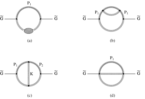
Figure 6: Contributions to the gravitino self energy.

The gravitino self-energy takes the form (cf. eq. (10)),

$$\Sigma(P) \propto {1\over M^{2}}\mbox{tr}{\left[\Pi_{\mu\nu}(P)S(P)^{\nu}\ldots\overline{S}^{\mu}(P)\right]}$$ (A.2)

$$\propto {1\over M^{2}}\mbox{tr}\left[(-/\!\!\!\!P)[\gamma^{\nu},\gamma^{\rho}]\gamma^{\mu}\lambda^{a}(P_{1})F^{a}_{\nu\rho}(K_{1})\ldots F^{b}_{\tau\sigma}(K_{1})\overline{\lambda}^{b}(P_{1})\gamma_{\mu}[\gamma^{\tau},\gamma^{\sigma}]\right]$$

$$+{2m_{\tilde{g}}^{2}\over 3m_{\tilde{G}}^{2}M^{2}}\mbox{tr}\left[[\gamma^{\nu},\gamma^{\rho}]\lambda^{a}(P_{1})F_{\nu\rho}(K_{1})\ldots F_{\tau\sigma}(K_{1})\overline{\lambda}^{a}(P_{1})[\gamma^{\tau},\gamma^{\sigma}]\right]\;.$$

The one- and two-loop contributions for the pure gauge theory in resummed perturbation theory are depicted in Fig. (6). The contributions (a) and (b) represent for the gluino line the first two terms of the gluino propagator. This corresponds to the substitution,

$$\lambda(P_{1})\ldots\overline{\lambda}(P_{1})\rightarrow/\!\!\!\!P_{1}A(P_{1},v)+/\!\!\!\!vB(P_{1},v)\;.$$ (A.3)

This is the general form of the gluino propagator for $m_{\tilde{g}}=0$ because of chiral symmetry and the fact that the velocity $v$ appearing in the gluon propagator is the only other vector available apart from the momentum $P_{1}$. With

$$\gamma^{\mu}\gamma^{\nu}\gamma_{\mu}=-2\gamma^{\nu}$$ (A.4)

one then reads off the factor (A.1) for the contributions (a) and (b). The same arguments apply for the contribution Fig. (6d).

For Fig. (6c) one obtains for the gluino line,

$$\lambda(P_{1})\ldots\overline{\lambda}(P_{1})\rightarrow/\!\!\!\!P_{1}\gamma^{\nu}/\!\!\!\!P_{2}\;.$$ (A.5)

With

$$\gamma^{\mu}/\!\!\!\!P_{1}\gamma^{\nu}/\!\!\!\!P_{2}\gamma_{\mu}=-2/\!\!\!\!P_{2}\gamma^{\nu}/\!\!\!\!P_{1}\;,$$ (A.6)

the interchange $P_{1}\leftrightarrow P_{2}$ and the property of the gluon propagator $\Delta(-K)=\Delta(K)$ one obtains the factor (A.1) also for this contribution.

Appendix B

In this appendix we explain the calculation of the contribution of hard virtual photons to the axion production rate $\Gamma_{a}^{\rm hard}(E)$. We start by reconsidering the defining equation (23):

$$n_{B}(E)\Gamma_{a}^{\rm hard}(E) = 2\int{d\Omega_{p}\over 4\pi}{1\over 2E}\int\left[\prod_{i=1}^{3}\frac{d^{3}p_{i}}{(2\pi)^{3}2E_{i}}\right](2\pi)^{4}\delta^{4}(P_{1}+P_{2}-P-P_{3})$$ (B.1)

$$\ \ n_{\rm total}^{FBF}|M|^{2}\Theta(|{\bf p}_{1}-{\bf p}_{3}|-k_{\rm cut})\;$$

where the matrix element squared for $e^{-}\gamma\to e^{-}a$ is given in Eq. (24) and

$$n_{\rm total}^{FBF}=n_{F}(E_{1})n_{B}(E_{2})(1-n_{F}(E_{3})).$$ (B.2)

A great simplification is achieved in the computation of (B.1) if one uses as reference momentum the difference vector ${\bf k}={\bf p}_{1}-{\bf p}_{3}$, i.e., we write

$$\frac{d^{3}p_{1}}{2E_{1}} = \delta(P_{1}^{2})\Theta(E_{1})dE_{1}d^{3}p_{1}$$ (B.3)

$$= \int d^{3}k\delta^{3}({\bf k}+{\bf p}_{3}-{\bf p}_{1})\delta(P_{1}^{2})\Theta(E_{1})dE_{1}d^{3}p_{1}$$

$$= \delta(E_{1}^{2}-|{\bf k}+{\bf p}_{3}|^{2})\Theta(E_{1})dE_{1}d^{3}k.$$

Further,

$$\frac{d^{3}p_{2}}{2E_{2}}\delta^{4}(P_{1}+P_{2}-P-P_{3}) = \delta(P_{2}^{2})\Theta(E_{2})d^{4}P_{2}\delta^{4}(P_{1}+P_{2}-P-P_{3})$$ (B.4)

$$= \delta((E+E_{3}-E_{1})^{2}-({\bf p}-{\bf k})^{2})\Theta(E+E_{3}-E_{1}).$$

We now use rotational invariance to choose

$${\bf k} = k\ (0,0,1),$$

$${\bf p} = E\ (0,\sin\tilde{\theta},\cos\tilde{\theta}),$$

$${\bf p}_{3} = E_{3}\ (\cos\phi\sin\theta,\sin\phi\sin\theta,\cos\theta),$$ (B.5)

which implies

$$s = (P_{1}+P_{2})^{2}=(P+P_{3})^{2}=2EE_{3}(1-\sin\theta\sin\phi\sin\tilde{\theta}-\cos\theta\cos\tilde{\theta}),$$

$$t = (P_{1}-P_{3})^{2}=(E_{1}-E_{3})^{2}-k^{2},$$ (B.6)

and

$$|{\bf k}+{\bf p}_{3}|^{2} = E_{3}^{2}+k^{2}+2E_{3}k\cos\theta,$$

$$|{\bf p}-{\bf k}|^{2} = E^{2}+k^{2}-2Ek\cos\tilde{\theta}.$$ (B.7)

It follows that

$$\delta((E+E_{3}-E_{1})^{2}-({\bf p}-{\bf k})^{2}) = \frac{1}{2kE}\delta\left(\cos\tilde{\theta}-\frac{E^{2}+k^{2}-(E+E_{3}-E_{1})^{2}}{2kE}\right),$$

$$\delta(E_{1}^{2}-|{\bf k}+{\bf p}_{3}|^{2}) = \frac{1}{2kE_{3}}\delta\left(\cos\theta-\frac{E_{1}^{2}-E_{3}^{2}-k^{2}}{2kE_{3}}\right).$$ (B.8)

The integrations over the $\delta$-functions yield the following $\Theta$-functions (where we use also the $\Theta$-functions $\Theta(E_{1}),\Theta(E+E_{3}-E_{1})$ and $E=p>0,E_{3}=p_{3}>0$:
1.) From the integration over $\cos\theta$ we get:

$$\cos\theta<1 \rightarrow k>E_{1}-E_{3},$$

$$\cos\theta>-1 \rightarrow E_{1}>|E_{3}-k|.$$ (B.9)

The second of these constraints is equivalent to

$$E_{3}-E_{1}<k<E_{1}+E_{3}.$$ (B.10)

2.) From the integration over $\cos\tilde{\theta}$ we get:

$$\cos\tilde{\theta}<1 \rightarrow |E-k|<E+E_{3}-E_{1},$$

$$\cos\tilde{\theta}>-1 \rightarrow k>E_{3}-E_{1}.$$ (B.11)

The first of these constraints is equivalent to

$$E_{1}-E_{3}<k<2E+E_{3}-E_{1}.$$ (B.12)

After integrating out the $\delta$-functions we therefore have:

$$n_{B}(E)\Gamma_{a}^{\rm hard}(E)=\frac{1}{2^{7}\pi^{4}}\frac{1}{E^{2}}\int dE_{1}dE_{3}n_{\rm total}^{FBF}dkd\phi|M|^{2}\Omega,$$ (B.13)

where $\Omega$ is the product of all $\Theta$-functions that restrict the integrations over $E_{1},E_{3}$ and $k$,

$$\Omega = \Theta(k-k_{\rm cut})\Theta(k-|E_{1}-E_{3}|)$$ (B.14)

$$\Theta(E_{1}+E_{3}-k)\Theta(2E+E_{3}-E_{1}-k)$$

$$\Theta(E_{1})\Theta(E_{3})\Theta(E+E_{3}-E_{1})\;.$$

Since only $s$ depends on $\phi$, we can integrate out also this angle without difficulty:

$$\int d\phi|M|^{2} = \frac{e^{2}}{f^{2}}\int d\phi\left(\frac{-2s^{2}}{t}-2s-t\right)$$ (B.15)

$$= \frac{3e^{2}\pi}{2f^{2}}\left[(E_{1}-E_{3})^{2}-k^{2}\right]\left(-1+\frac{2}{3}\frac{E_{1}^{2}+E_{3}^{2}+2EE_{2}}{k^{2}}\right.$$

$$\left.-\frac{(E_{3}+E_{1})^{2}(E+E_{2})^{2}}{k^{4}}\right)\equiv g.$$

We thereby obtain the result given in Eq. (26) in the main text. We now rewrite the expression for (B.14) using

$$\Theta(E_{1}+E_{3}-k)=1-\Theta(k-E_{1}-E_{3}).$$ (B.16)

We use $\Theta(k-E_{1}-E_{3})\Theta(k-|E_{1}-E_{3}|)=\Theta(k-E_{1}-E_{3})$ and thus get

$$\Omega = \Big{[}\Theta(k-k_{\rm cut})\Theta(k-|E_{1}-E_{3}|)\Theta(2E+E_{3}-E_{1}-k)$$ (B.17)

$$- \Theta(k-k_{\rm cut})\Theta(k-E_{1}-E_{3})\Theta(2E+E_{3}-E_{1}-k)\Big{]}$$

$$\times \Theta(E_{1})\Theta(E_{3})\Theta(E+E_{3}-E_{1}).$$

We multiply the second term in the brackets of Eq. (B.17) with 1:

$$1=\Theta(k_{\rm cut}-E_{1}-E_{3})+\Theta(E_{1}+E_{3}-k_{\rm cut}),$$ (B.18)

and note that

$$\Theta(k-k_{\rm cut})\Theta(k-E_{1}-E_{3})\Theta(k_{\rm cut}-E_{1}-E_{3})$$

$$= \Theta(k-k_{\rm cut})\Theta(k_{\rm cut}-E_{1}-E_{3}),$$ (B.19)

and

$$\Theta(k-k_{\rm cut})\Theta(k-E_{1}-E_{3})\Theta(E_{1}+E_{3}-k_{\rm cut})$$

$$= \Theta(k-E_{1}-E_{3})\Theta(E_{1}+E_{3}-k_{\rm cut}).$$ (B.20)

The contribution from the first term on the r.h.s. of Eq. (B.18) is zero in the limit $k_{\rm cut}\to 0$. We see this by integrating over $k$ from $k_{\rm cut}$ to $2E+E_{3}-E_{1}$. The resulting expression has terms $\sim 1/k_{\rm cut}^{3}$, $\sim 1/k_{\rm cut}^{1}$. Since from $k_{\rm cut}>E_{1}+E_{3}$ it follows that both $E_{1}$ and $E_{3}$ are smaller than $k_{\rm cut}$ it is easy to see by power counting that the expression after the $k$ integration is of order $k_{\rm cut}$. Then we are left to consider:

$$n_{B}(E)\Gamma_{a}^{\rm hard}(E)=g_{1}+g_{2},$$ (B.21)

where

$$g_{1} = \frac{1}{2^{7}\pi^{4}}\frac{1}{E^{2}}\int_{0}^{\infty}dE_{3}\int_{0}^{\infty}dE_{1}n_{\rm total}^{FBF}\Theta(E+E_{3}-E_{1})$$

$$\times \int dk\Theta(k-k_{\rm cut})\Theta(k-|E_{1}-E_{3}|)\Theta(2E+E_{3}-E_{1}-k)g,$$

$$g_{2} = -\frac{1}{2^{7}\pi^{4}}\frac{1}{E^{2}}\int_{0}^{\infty}dE_{3}\int_{0}^{\infty}dE_{1}n_{\rm total}^{FBF}\Theta(E+E_{3}-E_{1})\Theta(E_{1}+E_{3}-k_{\rm cut})$$ (B.22)

$$\times \int dk\Theta(k-E_{1}-E_{3})\Theta(2E+E_{3}-E_{1}-k)g,$$

The integral over $k$ in $g_{2}$ is nonzero only if

$$E_{1}+E_{3}<2E+E_{3}-E_{1}\Leftrightarrow E_{1}<E.$$ (B.23)

In the limit $k_{\rm cut}\to 0$ we therefore get:

$$g_{2}=\frac{e^{2}}{16\pi^{3}f^{2}}\frac{1}{E^{2}}\int_{0}^{\infty}dE_{3}\int_{0}^{E}dE_{1}n_{\rm total}^{FBF}(E_{1}-E)\left[(E+E_{1})E_{3}+E_{1}(E-E_{1})\right],$$ (B.24)

We rewrite this result for later use as follows:

$$g_{2} = \frac{e^{2}}{16\pi^{3}f^{2}}\frac{1}{E^{2}}\int_{0}^{\infty}dE_{3}\int_{0}^{E+E_{3}}dE_{1}\ln\left(\frac{|E_{1}-E_{3}|}{E_{3}}\right)$$

$$\times \Theta(E-E_{1})\frac{d}{dE_{1}}\left[n_{\rm total}^{FBF}(E_{1}^{2}E_{2}^{2}-E^{2}E_{3}^{2})\right].$$

We now turn towards the computation of $g_{1}$. We first multiply by 1:

$$g_{1}=g_{1}\Theta(k_{\rm cut}-|E_{1}-E_{3}|)+g_{1}\Theta(|E_{1}-E_{3}|-k_{\rm cut})\equiv g_{11}+g_{12}$$ (B.26)

Note that

$$\Theta(k-k_{\rm cut})\Theta(k-|E_{1}-E_{3}|)\Theta(k_{\rm cut}-|E_{1}-E_{3}|)$$

$$= \Theta(k-k_{\rm cut})\Theta(k_{\rm cut}-|E_{1}-E_{3}|)$$ (B.27)

and

$$\Theta(k-k_{\rm cut})\Theta(k-|E_{1}-E_{3}|)\Theta(|E_{1}-E_{3}|-k_{\rm cut})$$

$$= \Theta(k-|E_{1}-E_{3}|)\Theta(|E_{1}-E_{3}|-k_{\rm cut}).$$ (B.28)

We therefore have

$$g_{11} = \frac{1}{2^{7}\pi^{4}}\frac{1}{E^{2}}\int_{0}^{\infty}dE_{3}\int_{0}^{\infty}dE_{1}n_{\rm total}^{FBF}\Theta(E+E_{3}-E_{1})\Theta(k_{\rm cut}-|E_{1}-E_{3}|)$$ (B.29)

$$\times \int dk\Theta(k-k_{\rm cut})\Theta(2E+E_{3}-E_{1}-k)g$$

$$g_{12} = \frac{1}{2^{7}\pi^{4}}\frac{1}{E^{2}}\int_{0}^{\infty}dE_{3}\int_{0}^{\infty}dE_{1}n_{\rm total}^{FBF}\Theta(E+E_{3}-E_{1})\Theta(|E_{1}-E_{3}|-k_{\rm cut})$$ (B.30)

$$\times \int dk\Theta(k-|E_{1}-E_{3}|)\Theta(2E+E_{3}-E_{1}-k)g.$$

Consider first $g_{11}$. The integration of $g$ over $k$ can be carried out easily. We do not write down the result explicitly but note that it contains terms $\sim 1/k_{\rm cut}^{3}$ and $\sim 1/k_{\rm cut}$. The integration over $E_{1}$ is done next. From $k_{\rm cut}>|E_{1}-E_{3}|$ we get

$$E_{3}-k_{\rm cut}<E_{1}<E_{3}+k_{\rm cut}.$$ (B.31)

In the limit $k_{\rm cut}\to 0$ we can therefore set $E_{1}=E_{3}$ in the distribution functions $n_{\rm total}^{FBF}$ and get

$$g_{11} = \frac{e^{2}}{3\pi^{3}f^{2}}n_{B}(E)\int_{0}^{\infty}dE_{3}E_{3}^{2}n_{F}(E_{3})(1-n_{F}(E_{3}))$$ (B.32)

$$= \frac{e^{2}T^{3}}{18\pi f^{2}}n_{B}(E).$$

Now we turn towards the computation of $g_{12}$. We insert

$$1=\Theta(E_{1}-E_{3})+\Theta(E_{3}-E_{1}).$$ (B.33)

Then $g_{12}=g_{121}+g_{122}$ with

$$g_{121} = \frac{1}{2^{7}\pi^{4}}\frac{1}{E^{2}}\int_{0}^{\infty}dE_{3}\int_{0}^{\infty}dE_{1}n_{\rm total}^{FBF}\Theta(E+E_{3}-E_{1})\Theta(E_{1}-E_{3}-k_{\rm cut})$$

$$\times \int dk\Theta(k-E_{1}+E_{3})\Theta(2E+E_{3}-E_{1}-k)g,$$

$$g_{122} = \frac{1}{2^{7}\pi^{4}}\frac{1}{E^{2}}\int_{0}^{\infty}dE_{3}\int_{0}^{\infty}dE_{1}n_{\rm total}^{FBF}\Theta(E_{3}-E_{1}-k_{\rm cut})$$ (B.34)

$$\times \int dk\Theta(k-E_{3}+E_{1})\Theta(2E+E_{3}-E_{1}-k)g.$$

The integration over $k$ gives

$$g_{121} = \frac{e^{2}}{16\pi^{3}f^{2}}\frac{1}{E^{2}}\int_{0}^{\infty}dE_{3}\int_{E_{3}+k_{\rm cut}}^{E_{3}+E}dE_{1}n_{\rm total}^{FBF}\frac{(E_{1}^{2}+E_{3}^{2})E_{2}^{2}}{E_{1}-E_{3}},$$

$$g_{122} = -\frac{e^{2}}{16\pi^{3}f^{2}}\frac{1}{E^{2}}\int_{0}^{\infty}dE_{3}\int_{0}^{E_{3}-k_{\rm cut}}dE_{1}n_{\rm total}^{FBF}\frac{E^{2}(E_{1}^{2}+E_{3}^{2})}{E_{1}-E_{3}}.$$ (B.35)

The logarithmic dependence on $k_{\rm cut}$ is extracted by a partial integration with $f^{\prime}(E_{1})=1/(E_{1}-E_{3}),\ f(E_{1})=\ln\left(|E_{1}-E_{3}|/E_{3}\right)$.

For the surface term we get:

$$g_{\rm surface} = -\frac{e^{2}}{4\pi^{3}f^{2}}n_{B}(E)\int_{0}^{\infty}dE_{3}\ln\left(\frac{k_{\rm cut}}{E_{3}}\right)\frac{E_{3}^{2}\exp(E_{3}/T)}{(\exp(E_{3}/T)+1)^{2}}$$ (B.36)

$$= \frac{e^{2}T^{3}}{24\pi f^{2}}n_{B}(E)\left[\ln\left(\frac{2T}{k_{\rm cut}}\right)+\frac{3}{2}-\gamma+\frac{\zeta^{\prime}(2)}{\zeta(2)}\right]$$

In the remaining term, which is given by $-\int dE_{1}f(E_{1})g^{\prime}(E_{1})$, $k_{\rm cut}$ can be set to zero. Writing $g_{12}=g_{\rm surface}+g_{\rm partial}$ we obtain:

$$g_{\rm partial} = -\frac{e^{2}}{16\pi^{3}f^{2}}\frac{1}{E^{2}}\int_{0}^{\infty}dE_{3}\int_{0}^{\infty}dE_{1}\Theta(E+E_{3}-E_{1})\ln\left(\frac{|E_{1}-E_{3}|}{E_{3}}\right)$$ (B.37)

$$\times \Bigg{\{}\Theta(E_{1}-E_{3})\frac{d}{dE_{1}}\left[n_{\rm total}^{FBF}E_{2}^{2}(E_{1}^{2}+E_{3}^{2})\right]$$

$$- \Theta(E_{3}-E_{1})\frac{d}{dE_{1}}\left[n_{\rm total}^{FBF}E^{2}(E_{1}^{2}+E_{3}^{2})\right]\Bigg{\}}$$

Performing the differentiation and combining the results for $g_{1}$ and $g_{2}$ leads to the final result Eq. (28) given in the main text.

Appendix C

In this appendix we describe in some detail the calculation of the hard virtual gluon contribution and of the other non-singular contributions to the gravitino production rate $\Gamma_{\tilde{G}}^{\rm hard}(E)$. We start by considering the defining equation (4). By summing the corresponding squared matrix elements of table 1 with the appropiate multiplicities and statistical factors, we get

$$|M_{BBF}|^{2} = \left(1+\frac{m^{2}_{\tilde{g}}}{3m^{2}_{\tilde{G}}}\right)\frac{2g^{2}(N^{2}-1)}{M^{2}}\left[\left(s+2t+\frac{2t^{2}}{s}\right)\left(N+n_{f}\right)+2sn_{f}\right],$$ (C.1)

$$|M_{BFB}|^{2} = \left(1+\frac{m^{2}_{\tilde{g}}}{3m^{2}_{\tilde{G}}}\right)\frac{4g^{2}(N^{2}-1)}{M^{2}}\left[\left(-t-2s-\frac{2s^{2}}{t}\right)\left(N+n_{f}\right)-2tn_{f}\right],$$ (C.2)

$$|M_{FFF}|^{2} = \left(1+\frac{m^{2}_{\tilde{g}}}{3m^{2}_{\tilde{G}}}\right)\frac{4g^{2}(N^{2}-1)}{M^{2}}\left(-t-2s-\frac{s^{2}}{t}+\frac{s^{2}}{t+s}-\frac{t^{2}}{s}\right)\left(N+n_{f}\right).$$ (C.3)

First we note that since $s=-t-u$ we may write $s+2t=t-u$ and

$$-\frac{s^{2}}{t}+\frac{s^{2}}{s+t}=-\frac{s^{2}}{t}-\frac{s^{2}}{u}.$$ (C.4)

The difference $t-u$ and $1/t-1/u$ is odd under exchanging $P_{1}$ and $P_{2}$. If the remaining integrand and the measure is even under this transformation, the integral over such terms will be zero. Therefore in $|M_{BBF}|^{2}$, the contribution of $s+2t$ will give zero. Further we may trade $s$ in $|M_{BBF}|^{2}$ with $-2t$. In $|M_{FFF}|^{2}$, we may likewise substitute

$$-\frac{s^{2}}{t}+\frac{s^{2}}{s+t}\to-\frac{2s^{2}}{t}.$$ (C.5)

Therefore only the following squared matrix elements have to be considered:

$$|M_{1}|^{2} = -t-2s-\frac{2s^{2}}{t},$$

$$|M_{2}|^{2} = t,$$

$$|M_{3}|^{2} = \frac{t^{2}}{s},$$ (C.6)

and we replace the matrix elements in (4) by

$$|M_{BBF}|^{2} \to \left(1+\frac{m^{2}_{\tilde{g}}}{3m^{2}_{\tilde{G}}}\right)\frac{4g^{2}(N^{2}-1)}{M^{2}}\left[|M_{3}|^{3}\left(N+n_{f}\right)-2|M_{2}|^{2}n_{f}\right],$$ (C.7)

$$|M_{BFB}|^{2} = \left(1+\frac{m^{2}_{\tilde{g}}}{3m^{2}_{\tilde{G}}}\right)\frac{4g^{2}(N^{2}-1)}{M^{2}}\left[|M_{1}|^{2}\left(N+n_{f}\right)-2|M_{2}|^{2}n_{f}\right],$$ (C.8)

$$|M_{FFF}|^{2} \to \left(1+\frac{m^{2}_{\tilde{g}}}{3m^{2}_{\tilde{G}}}\right)\frac{4g^{2}(N^{2}-1)}{M^{2}}\left(|M_{1}|^{2}-|M_{3}|^{2}\right)\left(N+n_{f}\right).$$ (C.9)

$|M_{1}|^{2}$ is the axion matrix element which has been discussed in appendix B. The different statistical factors in the case of gravitino production do not change the structure of the contribution from $|M_{1}|^{2}$ as compared to the axion case. Again we can extract the logarithmic dependence on the cutoff $k_{\rm cut}$ by a partial integration. In the case of BFB, the surface term contains an additional term which depends on the energy of the gravitino, see Eq. (C.14) below. The other two matrix elements do not induce a logarithmic dependence on the cutoff $k_{\rm cut}$, i.e. one can set $k_{\rm cut}=0$ to compute their contribution to the gravitino production rate. The contribution from $|M_{2}|^{2}=t$ can be obtained easily using the same methods as in the axion case, where now no partial integration is needed. We obtain

$$I_{BBF(BFB)}^{t} = \int{d\Omega_{p}\over 4\pi}{1\over 2E}\int\left[\prod_{i=1}^{3}\frac{d^{3}p_{i}}{(2\pi)^{3}2E_{i}}\right](2\pi)^{4}\delta^{4}(P_{1}+P_{2}-P-P_{3})n_{BBF(BFB)}|M_{2}|^{2}$$ (C.10)

$$= \frac{1}{96\pi^{3}}\int_{0}^{\infty}dE_{3}\int_{0}^{E+E_{3}}dE_{1}n_{BBF(BFB)}$$

$$\times \Bigg{\{}\Theta(E-E_{1})\frac{E-E_{1}}{E^{2}}\left[2E^{2}+(3E_{3}-E_{1})(E+E_{1})\right]$$

$$- \Theta(E_{1}-E_{3})\frac{E_{2}^{2}}{E^{2}}(2E-E_{3}+E_{1})$$

$$+ \Theta(E_{3}-E_{1})(-3E_{3}+3E_{1}-2E)\Bigg{\}},$$

To compute the contribution from $|M_{3}|^{2}=\frac{t^{2}}{s}$ it is convenient to choose different coordinates to perform the angular integrations, namely

$${\bf q} \equiv {\bf p}+{\bf p_{3}}=q(0,0,1),$$

$${\bf p} = E\ (0,\sin\tilde{\theta},\cos\tilde{\theta}),$$

$${\bf p}_{2} = E_{2}\ (\cos\phi\sin\theta,\sin\phi\sin\theta,\cos\theta).$$ (C.11)

The calculation of this contribution to $\Gamma_{\tilde{G}}^{\rm hard}(E)$ then goes along similar lines as for the axion, i.e. the integration of the angular variables $\cos\theta,\cos\tilde{\theta}$ can be trivially performed using the $\delta-$functions. This leads to several constraints for the integration over $q$, which can be performed without problems. The final result is rather compact:

$$I_{BBF(FFF)}^{t^{2}/s} = \int{d\Omega_{p}\over 4\pi}{1\over 2E}\int\left[\prod_{i=1}^{3}\frac{d^{3}p_{i}}{(2\pi)^{3}2E_{i}}\right](2\pi)^{4}\delta^{4}(P_{1}+P_{2}-P-P_{3})n_{BBF(FFF)}|M_{3}|^{2}$$ (C.12)

$$= \frac{1}{32\pi^{3}}\int_{0}^{\infty}dE_{3}\int_{0}^{E+E_{3}}dE_{2}n_{BBF(FFF)}$$

$$\times \Bigg{\{}\frac{E_{2}^{2}}{E+E_{3}}+\Theta(E_{2}-E_{3})\frac{E_{3}-E_{2}}{E^{2}}\left[E_{3}(E_{3}-E_{2})+E(E_{3}+E_{2})\right]\Bigg{\}}.$$

The full result for $\Gamma_{\tilde{G}}^{\rm hard}(E)$ can be written as in Eq. (42) with

$$I_{BBF}=32\pi^{3}\left(e^{E/T}+1\right)\left[(N+n_{f})I_{BBF}^{t^{2}/s}-2n_{f}I_{BBF}^{t}\right],$$ (C.13)

$$I_{BFB}=T^{3}(N+n_{f})\left[{\rm Li}_{2}(-e^{-E/T})-\frac{\pi^{2}}{6}(1+8\ln(2))\right]-64\pi^{3}n_{f}\left(e^{E/T}+1\right)I_{BFB}^{t},$$ (C.14)

$$I_{FFF}=-32\pi^{3}\left(e^{E/T}+1\right)(N+n_{f})I_{FFF}^{t^{2}/s}.$$ (C.15)

The hard contribution to the collision term can be obtained by a numerical integration. Adding all the contributions we finally find:

$$C_{\tilde{G}}^{\rm hard}(T) = \int\frac{d^{3}p}{(2\pi)^{3}}n_{F}(E)\Gamma_{\tilde{G}}^{\rm hard}(E)$$ (C.16)

$$= \left(1+\frac{m^{2}_{\tilde{g}}}{3m^{2}_{\tilde{G}}}\right)\frac{3\zeta(3)g^{2}(N^{2}-1)T^{6}}{32\pi^{3}M^{2}}$$

$$\times \left\{(N+n_{f})\left[\ln\left(\frac{T^{2}}{k_{\rm cut}^{2}}\right)+1.7014\right]+0.5781n_{f}\right\},$$

which yields, after adding the soft contribution, our final result for the gravitino collision term (43).

Erratum

As recently pointed out by Pradler and Steffen (Phys. Rev. D 75 (2007) 023509 [hep-ph/0608344]), Eq. (C.14) has to be replaced by

$$I_{BFB}=-\frac{4}{3}\pi^{2}\ln(2)T^{3}(N+n_{f})-64\pi^{3}n_{f}\left(e^{E/T}+1\right)I_{BFB}^{t}\;.$$ (E.1)

The difference between Eqs. (C.14) and (E.1) is a non-vanishing surface term in the BFB case, which in the partial integration leading from (B.24) to (B.25) was overlooked.

As a consequence, the numerical factor multiplying $(N+n_{f})$ changes in Eq. (C.16) from 1.7014 to 1.8782. Correspondingly, also the numerical factor multiplying $(N+n_{f})$ in Eq. (44), and the overall factors in Eqs. (47) and (48) change. The corrected equations read

$$C_{\tilde{G}}(T) = \int{d^{3}p\over(2\pi)^{3}}n_{F}(E)\left(\Gamma_{\tilde{G}}^{\mbox{\tiny soft}}(E)+\Gamma_{\tilde{G}}^{\rm hard}(E)\right)$$ (E.2)

$$= \left(1+\frac{m_{\tilde{g}}^{2}}{3m_{\tilde{G}}^{2}}\right)\frac{3\zeta(3)g^{2}(N^{2}-1)T^{6}}{32\pi^{3}M^{2}}$$

$$\hskip 42.67912pt\Bigg{\{}\left[\ln\left(\frac{T^{2}}{m_{g}^{2}}\right)+0.4992\right](N+n_{f})+0.5781n_{f}\Bigg{\}}\;,$$

$$Y_{\tilde{G}}=1.4\cdot 10^{-10}\left(\frac{T_{R}}{10^{10}\,\mbox{GeV}}\right)\left(\frac{100\,\mbox{GeV}}{m_{\tilde{G}}}\right)^{2}\left(\frac{m_{\tilde{g}}(\mu)}{1\,\mbox{TeV}}\right)^{2}\;,$$ (E.3)

$$\Omega_{\tilde{G}}h^{2} = m_{\tilde{G}}Y_{\tilde{G}}(T)n_{\mathrm{rad}}(T)h^{2}\rho_{c}^{-1}$$ (E.4)

$$= 0.27\left(\frac{T_{R}}{10^{10}\,\mbox{GeV}}\right)\left(\frac{100\,\mbox{GeV}}{m_{\tilde{G}}}\right)\left(\frac{m_{\tilde{g}}(\mu)}{1\,\mbox{TeV}}\right)^{2}\;.$$

Compared to Eqs. (47) and (48), the gravitino abundance is increased by 30%. (Note that also the prefactor $1/(2\sqrt{6})$ in Eq. (33) has to be replaced by $1/(4\sqrt{6})$.)

We thank Josef Pradler and Frank Steffen for informing us about the error in our paper.

References

• [1] D. Z. Freedman, P. van Nieuwenhuizen, S. Ferrara, Phys. Rev. D13 (1976) 3214;
S. Deser, B. Zumino, Phys. Lett. B 62 (1976) 335
• [2] H. Pagels, J. R. Primack, Phys. Rev. Lett. 48 (1982) 223
• [3] S. Weinberg, Phys. Rev. Lett. 48 (1982) 1303
• [4] M. D. Khlopov, A. D. Linde, Phys. Lett. B 138 (1984) 265
• [5] J. Ellis, J. E. Kim, D. V. Nanopoulos, Phys. Lett. B 145 (1984) 181
• [6] T. Moroi, H. Murayama, M. Yamaguchi, Phys. Lett. B 303 (1993) 289
• [7] M. Bolz, W. Buchmüller, M. Plümacher, Phys. Lett. B 443 (1998) 209
• [8] E. Braaten, T. C. Yuan, Phys. Rev. Lett. 66 (1991) 2183
• [9] H. A. Weldon, Phys. Rev. D28 (1983) 2007
• [10] J. Ellis, D. V. Nanopoulos, K. A. Olive, S.-J. Rey, Astropart. Phys. 4 (1996) 371
• [11] J. Ellis, G. B. Gelmini, J. L. Lopez, D. V. Nanopoulos, S. Sarkar, Nucl. Phys. B373 (1992) 399
• [12] M. Kawasaki, T. Moroi, Progr. Theor. Phys. 93 (1995) 879
• [13] E. Holtmann, M. Kawasaki, K. Kohri, T. Moroi, Phys. Rev. 60 (1999) 023506
• [14] T. Gerghetta, G. F. Giudice, A. Riotto, Phys. Lett. B 446 (1999) 28
• [15] T. Asaka, K. Hamaguchi, K. Suzuki, Phys. Lett. B490 (2000) 136
• [16] T. Asaka, T. Yanagida, hep-ph/0006211
• [17] M. Fukugita, T. Yanagida, Phys. Lett. B 174 (1986) 45
• [18] For a recent review and references, see
W. Buchmüller, M. Plümacher, Neutrino Masses and the Baryon Asymmetry, hep-ph/0007176
• [19] J. Wess, J. Bagger, Supersymmetry and Supergravity, Princeton University Press, Princeton, New Jersey, 1992
• [20] T. Moroi, Ph.D. thesis, hep-ph/9503210
• [21] S. Weinberg, The Quantum Theory of Fields, Vol. III, Cambridge University Press, Cambridge, UK, 2000
• [22] P. Fayet, Phys. Lett. B 84 (1979) 421
• [23] T. E. Clark, S. T. Love, Phys. Rev. 54 (1996) 5723
• [24] T. Lee, G.-H. Wu, Phys. Lett. B 447 (1999) 83
• [25] V. P. Silin, Sov. Phys. JETP 11 (1960) 1136;
O. Kalashnikov, V. V. Klimov, Sov. J. Nucl. Phys. 31 (1980) 699;
V. V. Klimov, Sov. Phys. JETP 55 (1982) 199;
H. A. Weldon, Phys. Rev. D26 (1982) 1394; Annals Phys. 271 (1999) 141
• [26] R. D. Pisarski, Physica A 158 (1989) 146
• [27] E. Braaten, R. D. Pisarski, Nucl. Phys. B337 (1990) 569
• [28] A. Hart, M. Laine, O. Philipsen, Nucl. Phys. B586 (2000) 443
• [29] R. Kallosh, L. Kovman, A. Linde, A. van Proeyen, Phys. Rev. D61 (2000) 103503
• [30] G. F. Giudice, A. Riotto, I. Tkachev, JHEP 9911 (1999) 036
• [31] Review of Particle Physics, Eur. Phys. J. C 15 (2000) 1