Statistical model for pionic partons

N. G. Kelkar^a, and M. Nowakowski^b,

^a Nuclear Physics Division, Bhabha Atomic Research Centre,

Mumbai 400 085, India.

^b Departamento de Fisica, Universidad de Los Andes

A.A.4976, Bogota D.C., Colombia

We present a model for the structure of the pion. Based on ideas of a recently developed statistical model of the nucleon, we assume the pion to be a gas of partons. The finite-size corrections (FSC) are incorporated through two parameters. Using the same two FSC parameters for the proton and pion we reproduce quantitatively the data on $\pi^{-}N\rightarrow\mu^{+}\mu^{-}X$ Drell-Yan production and valence quark distribution of the pion.

PACS numbers: 12.40.Ee, 14.40.Aq, 14.65.-q
Keywords: pion structure function, parton distribution, statistical model, phenomenological models of the pion, finite-size effects

1 Introduction

Recently, a statistical model for the structure of the nucleon was proposed [1]. The nucleon was described as a non-interacting gas of valence quarks, sea quarks and gluons in equilibrium. This picture was then improved by adding finite-size corrections (FSC) to the expression for the parton density function (PDF). These finite size corrections take into account the fact that the gas is enclosed in a finite volume. The model was successful in reproducing a large body of polarized and unpolarized nucleon structure function data. Since the ideas from statistical mechanics worked well inside one hadron, namely the nucleon, it is quite motivating to test these ideas in other hadrons as well. However, compared to the vast amount of precise data available for the nucleon, much less is available for others. Among hadrons other than the nucleon, the pion is the most widely explored. There exist data on $\pi^{-}N\rightarrow\mu^{+}\mu^{-}X$ Drell-Yan production [2, 3] and prompt photon production in $\pi^{\pm}p\rightarrow\gamma X$ [4] which have been used by some groups [5, 6] to obtain parameterizations for PDFs of the pion. The Drell-Yan data constrains the shape of the pion valence densities and the prompt photon data constrains the pionic gluon distribution in the large-x region. These data are, however, not sufficient to fix the gluon and sea in the pion uniquely. The number of parameters appearing in the expressions for the PDFs obtained from such global fits are very large and with no physical meaning. Hence it is worth investigating the scope of a statistical model which has fewer parameters based on a physical interpretation.

In this Letter, we present a statistical model for the parton distributions in the pion. The expressions for the pion PDFs are written assuming the pion to be a gas of massless partons. These are then improved to include FSC as in the case of the nucleon. In principle the two parameters associated with the FSC can be determined theoretically [7]. However, these parameters are sensitive to the equation of motion employed, the boundary conditions on the wave function, shape of the enclosure and details such as whether the particles are strictly massless. In ref.[1], in the absence of a complete understanding of the nucleon as a QCD bound state, a practical approach was taken and the two parameters for the nucleon were determined by fitting unpolarized structure function $F_{2}(x,Q^{2})$ data at one value of $Q^{2}$. In the case of the pion, due to scarcity of precise experimental data giving direct information on the pion PDFs, we prefer to use as a first guess, the same parameters for the pion as in the case of the proton [1]. Interestingly, with these parameters we get good quantitative agreement with the available data on pion valence quark distribution and $\pi^{-}N\rightarrow\mu^{+}\mu^{-}X$ Drell-Yan production. The agreement with data is nearly as good as that obtained by the existing parameterizations [5, 6].

2 The model

We visualise the pion to be made up of a gas of massless partons in equlibrium at temperature $T$ in a spherical volume $V$ with radius $R$. The parton number density $dn^{i}/dx$ in the infinite momentum frame (IMF) and the density $dn/dE$ in the pion rest frame are related to each other by,

$${dn^{i}\over dx}={M^{2}x\over 2}\int^{M/2}_{xM/2}{dE\over E^{2}}~{}~{}{dn\over dE},$$ (1)

where the superscript $i$ refers to the IMF, $M$ is the pion mass and $E$ is the parton energy in the pion rest frame [1, 8]. Using the standard procedure in statistical mechanics to introduce the effects of the finite size of an enclosure, in the expression for the density of states [9] we write $dn/dE$ for the pion as,

$$dn/dE=g~{}f(E)~{}(VE^{2}/2\pi^{2}+aR^{2}E+bR),$$ (2)

where $g$ is the spin-color degeneracy factor, $f(E)$ is the usual Fermi or Bose distribution function $f(E)=\{\exp[(E-\mu)/T]\pm 1\}^{-1}$, $V$ is the pion volume and $R$ is the radius of a sphere with volume $V$. We take $R\,=\,\sqrt{5/3}\rho\,=\,1.07fm$, where $\rho$ is the root-mean-square radius of the pion [10]. The three terms in (2) are the volume, surface and curvature terms, respectively. The coefficients $a$ and $b$ are, in principle, the free parameters of the model. For reasons mentioned in the introduction, though $a$ and $b$ can be determined theoretically, we prefer to choose these values to be the same as those determined phenomenologically for the proton in ref.[1]. Theoretically this makes sense, as the values $a=-0.376$ and $b=0.504$ obtained from the fitting procedure in ref.[1] are close to the values ($a=-1/2$ and $b=3/2\pi$) determined theoretically by Morse and Ingard [7]. We will come back to this point at the end of the paper.

To determine the values of the temperature and chemical potentials appearing in the distribution function $f(E)$, we consider the fact that any model of the PDFs for the pion has to obey the number and momentum constraints, the former being motivated by the constituent quark picture for mesons at a low scale (this scale, being our input scale, should not be to too small as compared with $\Lambda_{QCD}$ to allow for the evolution of the partons densities, hence we choose it to be $Q_{0}^{2}=m_{N}^{2}$ where $m_{N}$ is the mass of the nucleon). If $n_{\alpha(\bar{\alpha})}$ denotes the number of quarks (antiquarks) of flavour $\alpha$, then in the case of a $\pi^{-}$ for example, the constraints can be given as,

$$n_{\bar{u}}\,-\,n_{u}\,=\,1$$ (3)

$$n_{d}\,-\,n_{\bar{d}}\,=\,1$$ (4)

$$n_{s}\,-\,n_{\bar{s}}\,=\,0$$ (5)

$$\sum_{q,\,\bar{q},\,g}\,(momentumfractions)\,=\,1.$$ (6)

The numbers $n_{\alpha(\bar{\alpha})}$ in eqs.(3-5) are obtained from eqs.(1) and (2) by integrating the appropriate $dn^{i}/dx$ over $x$. The momentum fractions are obtained by integrating $xdn^{i}/dx$ over $x$. The temperature $T$ and chemical potentials ($\mu$) appearing in eqs.(3-6) are then not free parameters. For a given set of parameters $a$ and $b$, they are determined uniquely by solving the four coupled non-linear eqs.(3-6).

Using the values of $a$ and $b$ mentioned above, we obtain $T=22$ MeV, $\mu_{d}=-\mu_{u}=162$ MeV and $\mu_{s}=0$ in the case of a negatively charged pion. The left and right hand sides of eqs.(3-6) with these values of T and $\mu$, agree with each other up to an accuracy of one part in $10^{6}$. The chemical potentials for antiquarks are determined by using the relation $\mu_{\bar{q}}=-\mu_{q}$. The model, described above, fixes the parton distributions in a pion uniquely at an input scale $Q_{0}$. It remains to put it to test and compare the predictions with available experimental data. In order to compare with data, the parton distributions are evolved to different $Q^{2}$ values using the standard DGLAP evolution equations at next-to-leading order, starting from the input scale $Q_{0}^{2}=m_{N}^{2}$.

3 Results and discussion

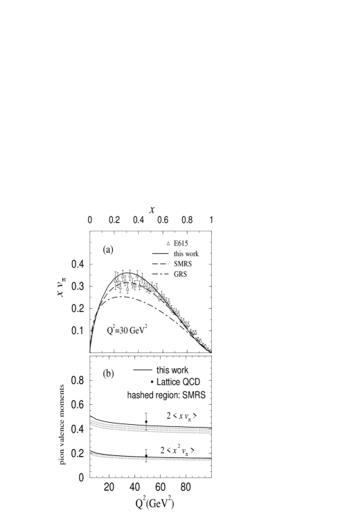
Figure 1: (a) Comparison of the valence structure function data from ref.[3] with the valence distribution within the statistical model (solid line). Dashed and dash-dotted lines are the valence densities obtained by the SMRS (ref.[5]) and GRS (ref.[6]) parameterizations respectively. (b) The first two moments of the pion valence distribution as predicted by the statistical model (solid line). Hashed region is the prediction [5] from the fit to Drell-Yan data of NA10 and the filled circles at $Q^{2}=49$ GeV² are lattice QCD [11] predictions.

To start with, we compare the $\pi^{-}$ valence quark distribution calculated within the statistical model with the available data at $Q^{2}=30$ GeV². In Fig. 1a we show the valence structure function extracted from $\pi^{-}W\rightarrow\mu^{+}\mu^{-}X$ Drell-Yan data by the E615 collaboration. The solid curve corresponding to our calculation of $xv_{\pi}=x(\bar{u}-u)$ done within the statistical model, shows reasonably good agreement with the E615 data. Our values of $xv_{\pi}$ are, however, higher than those due to the SMRS (dashed line) and GRS (dash-dotted line) parameterizations. Both these parameterizations have determined their valence densities by making a global fit to the $\pi N$ Drell-Yan data. To further compare our valence densities with other calculations, we calculate the first two moments of the pion valence quark distributions given by,

$$<\,x\,v_{\pi}\,>\,=\,\int_{0}^{1}\,x\,v_{\pi}(x)\,dx$$ (7)

$$<\,x^{2}\,v_{\pi}\,>\,=\,\int_{0}^{1}\,x^{2}\,v_{\pi}(x)\,dx.$$ (8)

In Fig. 1b we plot the $Q^{2}$ dependence of the pion valence moments. The solid curve corresponds to our calculation and the SMRS result is shown by the hashed region. The points with error bars are the results from a lattice QCD calculation [11] performed at $Q^{2}=49$ GeV².

Next, we put the statistical model to test with the $\pi^{-}N\rightarrow\mu^{+}\mu^{-}X$ Drell-Yan data. We calculate the double-differential cross-section $d^{2}\sigma/dx_{F}d\sqrt{\tau}$ where $x_{F}=x_{\pi}-x_{N}$ and $\sqrt{\tau}=x_{\pi}x_{N}=M^{2}/s$. At leading order, $x_{\pi}$ and $x_{N}$ are the Bjorken $x$ variables of the pion and target nucleon respectively. M is the invariant mass of the muon pair and $\sqrt{s}$ is the centre of mass energy. We calculate the Drell-Yan cross-sections using the full next-to-leading order expressions [5] and with the choice $Q^{2}=M^{2}$. The proton PDFs required for the calculation of the $\pi^{-}N$ Drell-Yan cross-sections are also calculated within the statistical model. Both the pion and nucleon PDFs are calculated using the same values of the FSC parameters $a$ and $b$. A detailed description of the evaluation of the nucleon PDFs can be found in ref.[1]. To take into account uncertainties due to normalization and higher order QCD corrections, we multiply our cross-sections by the standard $K^{\prime}$-factor. We analyse two different sets of data obtained from a $\pi^{-}$ beam incident on a tungsten target, $\pi^{-}W\rightarrow\mu^{+}\mu^{-}X$, by the NA10 and E615 collaboration. To make a correct comparison of our calculated cross-sections for $\pi^{-}N\rightarrow\mu^{+}\mu^{-}X$ with the $\pi^{-}W$ data, we multiply our cross-sections with a factor $R=-0.55x_{N}+1.1$. This form of the correction factor R is consistent with the observed values [12] of R as shown in ref.[5]. In Fig.2 we compare our calculated results with the NA10 data taken at $\pi^{-}$ beam momenta of 194 and 286 GeV/c. With $K^{\prime}$ factors of 1.02 and 1.06 at beam momenta 194 and 286 GeV/c respectively, we find reasonably good agreement with data at different values of $\sqrt{\tau}$. Our $K^{\prime}$ values are close to those in ref.[5] which range between 1.1 and 1.4 depending on the type of fit. A discussion on the $K^{\prime}$ factor can be found in ref.[13] where it was also noted that it should be fairly close to unity. In Fig.2 we also show the dependence of the cross sections on the choice of the parameters $a$ and $b$. The solid curves correspond to $a=-0.376$ and $b=0.504$ which are the values used throughout this work. Varying the parameters arbitrarily we found that the agreement with data reduces as we move away from the values of $a$ and $b$ quoted above. To demonstrate this fact, we plot the cross sections at beam momentum 286 GeV/c for two different sets of $a$ and $b$ in Fig. 2. The dashed curves correspond to the calculations with $a=-0.2$, $b=0.3$ and the dot-dashed curves correspond to those with $a=-0.6$, $b=0.7$.

In Fig.3 we show our calculations in comparison with the E615 data at $P_{L}=252$ GeV/c. The $K^{\prime}$ factor in this case is 0.85. It differs from the $K^{\prime}$ obtained by us for the NA10 data due to normalization errors in the data. Since the ratio $K^{\prime}(NA10)/K^{\prime}(E615)$ in this work is very similar to that obtained in refs.[5, 6], we do not worry about the fact that $K^{\prime}(E615)<1$. As mentioned above it could be due to errors in normalization. The agreement of our results with data is again quite good. We are, however, not able to reproduce data at very high or low values of $\sqrt{\tau}$ very well. Although the reason for this disagreement is not clear to us, it certainly is not a short-coming of the statistical model. We say so because this kind of disagreement was also found in ref.[5]. They included the data only in a certain range of $\sqrt{\tau}$ for fitting as they were unable to reproduce the data at very high and low values of $\sqrt{\tau}$.

Finally in Fig. 4 we compare the valence, sea and gluon distributions of the pion within the statistical model with those obtained by the SMRS and GRS parameterizations. Since the pion sea distributions are not well determined by data, the SMRS parameterization made different fits by varying the fraction of the pion momentum carried by the sea between 10% and 20%. Interestingly, we find that the sea calculated within the statistical model carries a fraction roughly equal to 15% of the pion momentum which is like the SMRS best fit value.

To summarize, we can say that we have presented a simple physical model for the pion, using ideas from statistical mechanics. The only parameters in the description of the pionic parton densities are the two ‘finite-size correction’ parameters. Considering the fact that the only two parameters appearing in the model for the pion have not been determined by any fit to the pionic data, the success of the model in reproducing data on the pion is surprising. Since we use the same parameters for the proton and pion (for reasons explained in the Introduction), we have in a sense, a unified model for the proton and pion. We tried different sets of the values $a$ and $b$ for the pionic partons and having the same values as that for the proton is an outcome of our work rather than an assumption. At this stage, however, it would be too early to speculate about the significance of this result. It could be that given a wealth of precise enough data on pionic parton distributions, the ‘true’ values of $a$ and $b$ determined by a fit, will differ from the ones presently used. However, it is clear from our results that the difference will not be drastic. It seems therefore that the values for $a$ and $b$ are always close to the theoretical values, $a=-1/2$ and $b=3/2\pi$ determined in ref. [7]. This could partly be the reason why the statistical model works so well for the proton as well as for the pion using the same $a$ and $b$. Further efforts to understand why the ideas from statistical mechanics work inside hadrons could be worthwhile and could improve our understanding of hadron structure. In future we intend to understand this point in more detail, by using for comparison a larger set of data (i.e. prompt photon production), by extending the model to other hadrons like kaons and hyperons, and relating their structure functions to fragmentation functions. This could also settle the issue about the parameters $a$ and $b$.

Acknowledgements
One of the authors (NGK) gratefully acknowledges the warm hospitality of the Physics Group at Universidad de Los Andes.

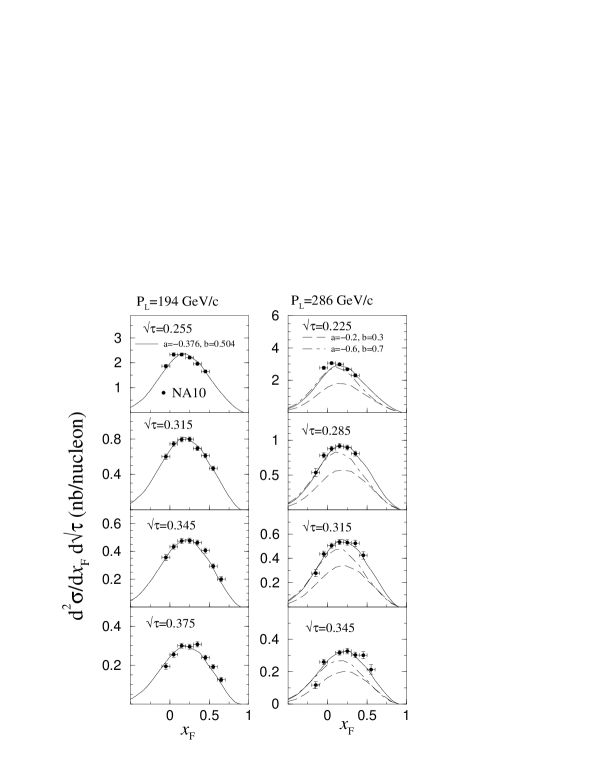
Figure 2: Drell-Yan data for $\pi^{-}W\rightarrow\mu^{+}\mu^{-}X$ at beam momenta of 194 (left column) and 286 GeV/c (right column) taken by the NA10 collaboration [2]. Solid lines are the next-to-leading order cross section predictions within the statistical model with the finite-size correction parameters $a=-0.376$ and $b=0.504$ as used throughout this work. The dashed ($a=-0.2$, $b=0.3$) and dot-dashed lines ($a=-0.6$, $b=0.7$) at 286 GeV/c show the variation of the calculated cross sections with different choices of the parameters $a$ and $b$. The $K^{\prime}$ factors for the 194 and 286 GeV/c data are 1.02 and 1.06 respectively.

Figure 3: Drell-Yan cross section data for $\pi^{-}W\rightarrow\mu^{+}\mu^{-}X$ at beam momentum 252 GeV/c taken by the E615 collaboration [3]. Solid lines are the next-to-leading order cross section predictions within the statistical model with a $K^{\prime}$ factor of 0.85.

Figure 4: Comparison of the statistical model parton distributions (solid lines) with those due to the SMRS (ref.[5], dashed lines) and GRS (ref.[6], dash-dotted lines) parameterizations at $Q^{2}=30$ GeV².

References

- [1] R. S. Bhalerao, N. G. Kelkar, B. Ram, Phys. Lett. B 476 (2000) 285.
- [2] NA10 collaboration, B. Betev et al., Z. Phys. C 28 (1985) 9. The cross sections in this paper have been revised with a better estimate of the Fermi motion effects.
- [3] E615 collaboration, J. S. Conway et al., Phys. Rev. D 39 (1989) 92.
- [4] WA70 collaboration, M. Bonesini et al., Z. Phys. C 37 (1988) 535.
- [5] P. J. Sutton, A. D. Martin, W. J. Stirling, R. G. Roberts, Phys. Rev. D 45 (1992) 2349.
- [6] M. Glück, E. Reya, I. Schienbein, Eur. Phys. J. C 10 (1999) 313.
- [7] R. Balian, C. Bloch, Ann. of Phys. (N.Y.) 60 (1970) 401; R. K. Bhaduri, J. Dey, M. K. Srivastava, Phys. Rev. D 31 (1985) 1765; P. M. Morse, K. U. Ingard, Theoretical Acoustics (McGraw-Hill, New York, 1968) p. 587.
- [8] R. S. Bhalerao, Phys. Lett. B 380 (1996) 1; B 387 (1996) 881 (E).
- [9] D.L. Hill and J.A. Wheeler, Phys. Rev. 89 (1953) 1102; H.R. Jaqaman et al., Phys. Rev. C 29 (1984) 2067.
- [10] V. Bernard, N. Kaiser, Ulf-G. Meiner, Phys. Rev. C 62 (2000) 028201.
- [11] G. Martinelli, C. T. Sachrajda, Nucl. Phys. B 306 (1988) 865.
- [12] NA10 collaboration, P. Bordalo et al., Phys. Lett. B 193 (1987) 368.
- [13] G. Altarelli, S. Petrarca, F. Rapuano, Phys. Lett. B 373 (1996) 200.