A frequentist analysis of solar neutrino data

Abstract

We present a Monte Carlo analysis in terms of neutrino oscillations of the total rates measured in solar neutrino experiments in the framework of frequentist statistics. We show that the goodness of fit and the confidence level of the allowed regions in the space of the neutrino oscillation parameters are significantly overestimated in the standard method. We also present a calculation of exact allowed regions with correct frequentist coverage. We show that the exact VO, LMA and LOW regions are much larger than the standard ones and merge together giving an allowed band at large mixing angles for all $\Delta{m}^{2}\gtrsim 10^{-10}\,\mathrm{eV}^{2}$.

1 INTRODUCTION

Solar neutrino experiments [1] have observed a flux of neutrinos smaller than the one predicted by the Standard Solar Model (see, for example, Ref.[2]). Neutrino oscillations (see, for example, Ref.[3]) is widely considered to be the simplest and most attractive explanation of this anomaly. Assuming the simplest case of two-neutrino oscillations, the statistical analysis of solar neutrino data yields allowed regions for the oscillation parameters $\Delta m^{2}\equiv m_{2}^{2}-m_{1}^{2}$, where $m_{1}$ and $m_{2}$ are the two neutrino masses, and $\tan^{2}\theta$, where $\theta$ is the neutrino mixing angle.

The allowed regions in the $\tan^{2}\theta$–$\Delta m^{2}$ plane are usually determined through a least-square fit (see, for example, Refs.[4, 5]), in which the parameters are estimated through the minimum of the function

$$X^{2} = \sum_{j_{1},j_{2}=1}^{N_{\mathrm{exp}}}\left(R^{\mathrm{(thr)}}_{j_{1}}-R^{\mathrm{(exp)}}_{j_{1}}\right)(V^{-1})_{j_{1}j_{2}}$$ (1)

$$\hskip 28.45274pt\times\left(R^{\mathrm{(thr)}}_{j_{2}}-R^{\mathrm{(exp)}}_{j_{2}}\right)\,,$$

where $N_{\mathrm{exp}}=3$ is the number of experimental data points, $R^{\mathrm{(thr)}}_{j}$ and $R^{\mathrm{(exp)}}_{j}$ are the theoretical and experimental rates, respectively, and $V$ is the covariance matrix that accounts for experimental and theoretical uncertainties [6, 4, 7]. The theoretical rates $R^{\mathrm{(thr)}}_{j}$ and the covariance matrix $V$ depend on the parameters $\Delta m^{2}$, $\tan^{2}\theta$.

Usually, in the application of the least-squares method it is assumed that $X^{2}$ is distributed as a $\chi^{2}$ with $N_{\mathrm{exp}}=3$ degrees of freedom, $X^{2}_{\mathrm{min}}$ is distributed as a $\chi^{2}$ with $N_{\mathrm{exp}}-N_{\mathrm{par}}=1$ degrees of freedom, and $X^{2}-X^{2}_{\mathrm{min}}$ has a $\chi^{2}$ distribution with $N_{\mathrm{par}}=2$ degrees of freedom (see, for example, Ref.[9, 10]). This would be correct if: 1) the theoretical rates depended linearly on the parameters; 2) the errors of the differences between the theoretical and experimental rates were multinormally distributed with a constant covariance matrix. Actually, these requirements are not satisfied. In particular, it is well-known that the theoretical rates have a complicate dependence on the parameters. For example, in the simplest case of oscillations in vacuum the electron neutrino survival probability depends on $\Delta m^{2}$ through a sinusoidal function:

$$P_{\nu_{e}\to\nu_{e}}=1-\sin^{2}{2\theta}\sin^{2}{\left(\Delta m^{2}L/4E\right)}\,.$$ (2)

Moreover, the covariance matrix $V$ is not constant, but depends on $\Delta m^{2}$ and $\tan^{2}\theta$ (see Refs.[6, 4, 7]), and the errors of the differences between the theoretical and experimental rates are not multinormally distributed (this is due to the fact that each theoretical rate is given by the product of the neutrino flux times the experimental cross section; even if the errors of the neutrino flux and the errors of the experimental cross section are normally distributed, their product is not).

Since $X^{2}$ is not a $\chi^{2}$, in order to perform a reliable statistical analysis of the data it is necessary to calculate with a Monte Carlo the distribution of its minimum, $X^{2}_{\mathrm{min}}$, which is the estimator of the parameters $\Delta m^{2}$, $\tan^{2}\theta$.

In Section 2 we present the result of our Monte Carlo estimation of the goodness of fit and the confidence level (CL) of the standard allowed regions. In Section 3 we present a calculation of exact allowed region with correct frequentist coverage. A detailed explanation of our procedure and results has been presented in Ref. [8].

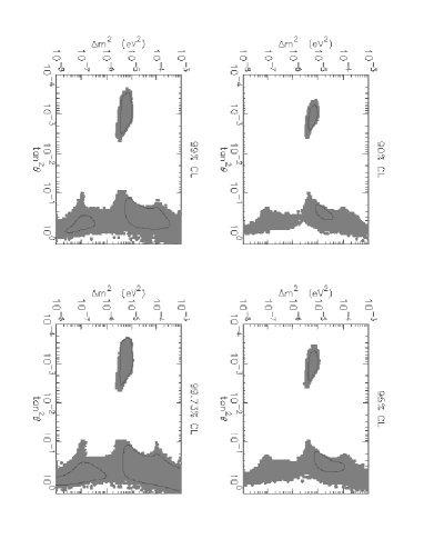
Figure 1: Allowed $90\%$, $95\%$, $99\%$, $99.73\%$ CL regions in the MSW part of the $\tan^{2}{\theta}$–$\Delta m^{2}$ plane. The gray areas are the allowed regions with exact frequentist coverage in the MSW region; the areas enclosed by the solid lines are the standard SMA, LMA and LOW allowed regions.

2 MONTE CARLO GOODNESS OF FIT AND CONFIDENCE LEVELS

The exact distribution of $X^{2}_{\mathrm{min}}$ is determined by the true value of the parameters $\Delta m^{2}$, $\tan^{2}\theta$, which are unknown. Nevertheless, it is possible to estimate the distribution assuming surrogates for the true value of the parameters. The most reasonable surrogates are the best-fit values $\widehat{\Delta m^{2}}$ and $\widehat{\tan^{2}{\theta}}$ (see, for example, Ref.[10]). Assuming $\widehat{\Delta m^{2}},\widehat{\tan^{2}{\theta}}$ as surrogates of the true values of the parameters, we generate $N_{S}$ synthetic data sets which simulate $N_{S}$ different independent sets of experiments. Using these sets we can estimate the goodness of fit and confidence levels of the standard allowed regions.

Goodness of fit is the probability to find in a set of hypothetical repeated experiments a $X^{2}_{\mathrm{min}}$ larger than the one actually observed.

From the rates analysis (with the 1999 data summarized in Ref.[5]), we find that, constraining the parameter in an area around the global minimum (which is the SMA region), the standard goodness of fit is reliable. This is due to the fact that in the neighborhood of the global minimum the dependence of the theoretical rates from the parameters is approximately linear and the covariance matrix is almost constant.

On the other hand, if the parameters are unconstrained (allowing all the MSW region with $10^{-8}\,\mathrm{eV}^{2}\lesssim\Delta{m}^{2}\lesssim 10^{-4}\,\mathrm{eV}^{2}$ and the VO region with $10^{-11}\,\mathrm{eV}^{2}\lesssim\Delta{m}^{2}\lesssim 10^{-8}\,\mathrm{eV}^{2}$), the goodness of fit is 40%, poorer than the 52% obtained with the standard method. The fit is worse! We conclude that the goodness of fit is overestimated by the standard procedure.

From the synthetic data sets we can also estimate the confidence level of the standard allowed regions. We start from the definition of confidence level of interval: it is the fractional number of intervals obtained in repeated experiments which cover the true values of parameters.

In the standard procedure the confidence intervals are determined by the condition

$$X^{2}\leq X^{2}_{\mathrm{min}}+\Delta\chi^{2}(\beta)\,,$$ (3)

where $\Delta\chi^{2}(\beta)$ is the value of $\chi^{2}$ such that the cumulative $\chi^{2}$ distribution for a number of degrees of freedom equal to the number of parameters is equal to the confidence level $\beta$. But this procedure would be correct only if $X^{2}$ were a $\chi^{2}$.

In our simulation, for a fixed $\beta$, we calculate the standard allowed regions for each synthetic data set. Then we count how many of them cover the surrogates of true values of parameters. This fraction is our estimate $\beta_{\mathrm{MC}}$ of the true confidence level of the standard allowed regions at $\beta$ CL.

We found that, if the parameters are constrained around the global minimum and there is only one standard $\beta$ CL allowed region, its confidence level $\beta_{\mathrm{MC}}$ is approximately equal to $\beta$. Instead, if the parameters are not constrained around the global minimum and there are several standard $\beta$ CL allowed regions, their confidence level $\beta_{\mathrm{MC}}$ is significantly smaller than $\beta$. For example, the Monte Carlo confidence level of the standard 90% CL allowed regions is only 86%.

This result was expected, because in the case of a real $\chi^{2}$ there is only one minimum that determines an elliptic allowed region, whereas $X^{2}$ has several local minima (especially in the vacuum oscillation region). Therefore, in repeated experiments there is a higher probability that the global minimum falls far from the assumed surrogates $\widehat{\Delta m^{2}}$, $\widehat{\tan^{2}{\theta}}$ of the true values of parameters, leading to a lower probability that the allowed regions cover $\widehat{\Delta m^{2}}$, $\widehat{\tan^{2}{\theta}}$.

The approach presented in this section allows to calculate only estimations of the goodness of fit and the confidence level of the standard allowed regions, because the calculation depends on the assumed surrogates of the true values of the parameters. In the next section we present the results of a calculation of allowed regions with exact confidence level, which is independent from the unknown true value of the parameters.

3 EXACT ALLOWED REGIONS

The construction of exact confidence intervals has been introduced by Neyman in 1937 (see, for example, Ref.[9, 11]). It guarantees that the resulting confidence intervals have correct frequentist coverage, i.e. they belong to a set of confidence intervals obtained with different or similar, real or hypothetical experiments that cover the true values of the parameters with the desired probability given by the chosen confidence level (see, for example, Ref.[12]). We apply this method in order to find confidence intervals with proper coverage for the neutrino oscillation parameters.

Starting with the choice of an appropriate estimator of the parameter under investigation, for any possible value of the parameter one calculates an acceptance interval with probability $\beta$, i.e. an interval of the estimator that contains $100\beta$% of the values of the estimator obtained in a large series of trials.

Once the $100\beta$% acceptance interval for each possible value of the parameter is calculated, the $100\beta$% confidence interval is simply composed by all the parameter values whose acceptance interval covers the measured value of the estimator.

This procedure can be generalized to the case of more parameters: the acceptance intervals (and also the confidence intervals) are multidimensional regions and could be composed by disjoint subintervals.

In the case of solar neutrino oscillations, we have two parameters, $\Delta m^{2}$ and $\tan^{2}{\theta}$, estimated through the minimum of $X^{2}$. We consider a grid with 5000 points in the MSW region and 6000 points in the VO region. For each point of the grid we generate about $6.5\times 10^{4}$ synthetic data sets that allow to calculate the distribution of the estimator $X^{2}_{\mathrm{min}}$ and the consequent acceptance regions. More details have been presented in Ref.[8].

Our results are shown in Figures 1 and 2, where we have plotted the $90\%$, $95\%$, $99\%$, $99.73\%$ CL regions in the MSW and VO parts of the $\tan^{2}{\theta}$–$\Delta m^{2}$ plane. One can see that the exact allowed regions are much larger than the standard ones. In particular, the LMA, LOW and VO regions are connected, giving an allowed band at large mixing angles for all $\Delta{m}^{2}\gtrsim 10^{-10}\,\mathrm{eV}^{2}$. Only the standard SMA region is a good approximation of the exact one.

Figure 2: Allowed $90\%$, $95\%$, $99\%$, $99.73\%$ CL regions in the VO part of the $\tan^{2}{\theta}$–$\Delta m^{2}$ plane. The gray areas are the allowed regions with exact frequentist coverage in the VO region; the areas enclosed by the solid lines are the standard VO allowed regions.

4 CONCLUSIONS

We have calculated with Monte Carlo the goodness of fit and the confidence level of the standard allowed regions of the two-neutrino oscillation parameters $\Delta m^{2}$ and $\tan^{2}{\theta}$ obtained from the fit of the total rates measured by solar neutrino experiments.

As expected, we found that the standard method overestimates the goodness of fit and the confidence level of the standard allowed regions.

Using Neyman’s construction, we have calculated exact allowed regions with correct frequentist coverage. We have shown that the exact VO, LMA and LOW regions are much larger than the standard ones and merge together giving an allowed band at large mixing angles for all $\Delta{m}^{2}\gtrsim 10^{-10}\,\mathrm{eV}^{2}$.

References

- [1] Homestake: B.T. Cleveland et al., Astrophys. J. 496, 505 (1998); Super-Kamiokande: M. Nakahata, Nucl. Phys. Proc. Suppl. 87, 125 (2000); GALLEX: W. Hampel et al., Phys. Lett. B447, 127 (1999); SAGE: J.N. Abdurashitov et al., Phys. Rev. C60, 055801 (1999).
- [2] J.N. Bahcall, Phys. Rept. 333-334, 47 (2000).
- [3] S.M. Bilenky, C. Giunti, and W. Grimus, Prog. Part. Nucl. Phys. 43, 1 (1999).
- [4] G.L. Fogli, E.Lisi, D. Montanino and A.Palazzo, Phys. Rev. D 62, 013002 (2000).
- [5] M.C. Gonzalez-Garcia et al., Nucl. Phys. B 573, 3 (2000).
- [6] G.L. Fogli and E.Lisi, Astropart. Phys. 3, 185 (1995).
- [7] M.V. Garzelli and C. Giunti, Phys. Lett. B488, 339 (2000), hep-ph/0006026.
- [8] M.V. Garzelli and C. Giunti, hep-ph/0007155.
- [9] W.T. Eadie et al., Statistical Methods in Experimental Physics, North Holland, Amsterdam, 1971.
- [10] W.H. Press et al., Numerical Recipes in C, Cambridge University Press, Second Edition, 1992.
- [11] C. Caso et al., Eur. Phys. J. C3, 1 (1998).
- [12] R.D. Cousins, AM. J. Phys. 63, 398 (1995).