Single charged Higgs boson production at next generation linear colliders

Abstract:

We study the single production of charged Higgs bosons in $e^{+}e^{-}$ collisions, chiefly in the Minimal Supersymmetric Standard Model. Our analysis complements foregoing studies of the pair production channel especially in regions where the kinematic constraint suppresses pair production. We present cross sections relevant to experiments at the next generation linear colliders and some brief discussions of their phenomenology. Our analysis shows that the single production is a useful alternative channel for studying the phenomenology of charged Higgs bosons, and there are regions of parameter space where it is accessible beyond the kinematic limit for pair production.

1 Introduction

Charged Higgs bosons $H^{\pm}$ are a cornerstone of beyond-the-Standard-Model phenomenology. They arise as a prediction of the supersymmetric extensions of the Standard Model (SM) from purely theoretical requirements of consistency. Their discovery and the confirmation of their properties will be a significant step towards a full understanding of electroweak symmetry breaking.

Some substantial effort has thus been channelled into the evaluation of their phenomenology at future colliders, and over the past few years the situation with respect to their discovery potential has become more clear.

At hadron colliders [1], especially with the luminosity of the LHC, charged Higgs bosons below the top quark mass are expected to be produced abundantly in the decay of top quarks. When their mass is near or greater than the top quark decay threshold, their discovery prospects are further hindered by the falling structure function but they will be produced mainly in the ‘$tb$-fusion’ process, namely the parton level process $gb\to tH^{-}$ and the charge conjugate. There have recently been attempts [2] to connect the two channels together by looking at a generic subprocess $gg\to t\bar{b}H^{-}$ which includes a component of the latter process that is leading order at large transverse momentum of the ‘spectator’ bottom quark. In both cases the most promising decay mode is presumably the $H^{-}\to\tau^{-}\bar{\nu}$ mode [3]. It is claimed that relatively heavy charged Higgs bosons, of mass up to 1 TeV, can be probed using this mode, especially at large $\tan\beta$, although a full experimental simulation similar to that presented in [4] will be essential to test this claim and to draw the discovery contour. Here $\tan\beta$ is as usual defined as the ratio of the vacuum expectation values of the two Higgs doublets. Several other production channels have also been considered [5].

At future electron-positron linear colliders (LCs), the dominant production process, if kinematically allowed, is the pair production process [6]:

$$e^{-}e^{+}\to H^{+}H^{-}.$$ (1)

The production rate depends only on the charged Higgs mass and the process provides a hallmark channel through which we can study $H^{\pm}$ phenomenology [7].

When the charged Higgs mass is near or above half the centre-of-mass energy the phenomenology is much less well understood. There has lately been some interest in the associated production mode with $W^{\pm}$ [8, 9, 10]:

$$e^{-}e^{+}\to H^{\pm}W^{\mp},$$ (2)

although the extent to which this channel could contribute towards the study of charged Higgs phenomenology is not clear. In models with a multi-Higgs-doublet structure, the process is loop-induced in the massless electron limit, and therefore the cross section is suppressed. We also note that no analysis of the SM background is available so far.

Other channels that have been studied in the literature are the heavy quark associated production mode [11]:

$$e^{-}e^{+}\to b\bar{b}W^{\pm}H^{\mp},$$ (3)

and the $\tau\nu_{\tau}$ associated production mode [12]:

$$e^{-}e^{+}\to H^{+}\tau^{-}\bar{\nu}_{\tau},H^{-}\tau^{+}\nu_{\tau}.$$ (4)

The purpose of this paper is to study the above processes in greater detail and to collect them together with many other single production channels of charged Higgs bosons in order to complement the pair production channel both above and below its kinematic threshold. Although our method is applicable generally in principle, we have adopted the Minimal Supersymmetric Standard Model (MSSM) for calculating Higgs masses and mixings. The MSSM being a model with a decoupling structure in the Higgs sector, the resulting cross sections are small compared to cases where, for example, extra resonances are available. However, it is beyond our intention to study models other than the MSSM in the present paper.

2 Production processes

We consider the following fourteen processes:

$$e^{-}e^{+} \to \tau^{-}\bar{\nu}_{\tau}H^{+},\tau^{+}\nu_{\tau}H^{-}$$ (5)

$$e^{-}e^{+} \to \bar{t}bH^{+},t\bar{b}H^{-}$$ (6)

$$e^{-}e^{+} \to W^{\mp}H^{\pm}\mathrm{(one\ loop)}$$ (7)

$$e^{-}e^{+} \to e^{-}\bar{\nu}H^{+},e^{+}\nu H^{-}\mathrm{(one\ loop)}$$ (8)

$$e^{-}e^{+} \to Z^{0}W^{\mp}H^{\pm}$$ (9)

$$e^{-}e^{+} \to h^{0}W^{\mp}H^{\pm}$$ (10)

$$e^{-}e^{+} \to H^{0}W^{\mp}H^{\pm}$$ (11)

$$e^{-}e^{+} \to A^{0}W^{\mp}H^{\pm}$$ (12)

$$e^{-}e^{+} \to e^{-}e^{+}W^{\mp}H^{\pm}$$ (13)

$$e^{-}e^{+} \to \nu_{e}\bar{\nu}_{e}W^{\mp}H^{\pm}$$ (14)

$$e^{-}e^{+} \to e^{-}\bar{\nu}_{e}Z^{0}H^{+},e^{+}\nu_{e}Z^{0}H^{-}$$ (15)

$$e^{-}e^{+} \to e^{-}\bar{\nu}_{e}h^{0}H^{+},e^{+}\nu_{e}h^{0}H^{-}$$ (16)

$$e^{-}e^{+} \to e^{-}\bar{\nu}_{e}H^{0}H^{+},e^{+}\nu_{e}H^{0}H^{-}$$ (17)

$$e^{-}e^{+} \to e^{-}\bar{\nu}_{e}A^{0}H^{+},e^{+}\nu_{e}A^{0}H^{-}.$$ (18)

The Feynman graphs corresponding to the above are shown in figure 1.

(a) processes (5) and (6)

(b) process (7). Shaded circles represent one-loop contributions.

(c) process (8). $W^{\pm}-H^{\pm}$ mixing is taken into account by using the renormalised couplings. We neglect the box diagram.

(d) process (9)

(e) processes (10)–(12)

(f) processes (13)–(15)

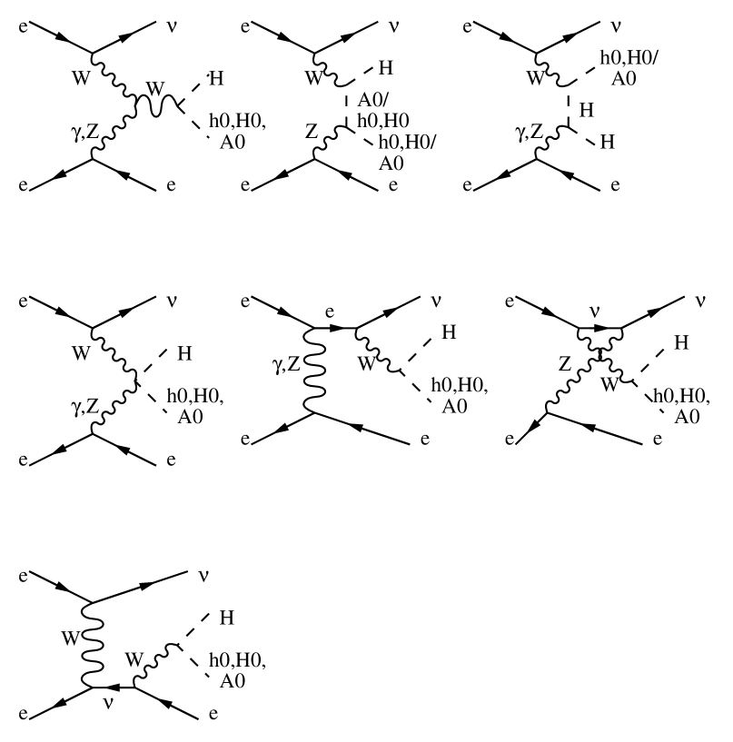
(g) processes (16)–(18)

Figure 1: Feynman diagrams for the single $H^{\pm}$ production processes. In all diagrams $H$ stands for $H^{\pm}$ and $W$ stands for $W^{\mp}$, the charge being dictated by charge conservation in the diagram concerned. Charge conjugated diagrams have been omitted from (b), (c) and (f) for simplicity.

For all tree-level processes, the matrix elements were calculated both by hand, for select set of diagrams in order to simplify the calculation, using the usual trace method, and by using the helicity amplitude formalism of [13]. The two sets of results agree up to the numerical precision employed. We present the matrix element squared for the dominant tree-level signal processes (5) and (6) in the appendix.

All processes were calculated at leading order only. For the 2HDM parameters, we adopted the MSSM throughout. For the SM parameters we adopted the following: $m_{b}=4.25$ GeV, $m_{t}=175$ GeV, $m_{e}=0.511$ MeV, $m_{\tau}=1.78$ GeV, $m_{\nu}=0$, $M_{W}=80.23$ GeV, $\Gamma_{W}=2.08$ GeV, $M_{Z}=91.19$ GeV, $\Gamma_{Z}=2.50$ GeV, $\sin^{2}\theta_{W}=0.232$. The top quark width $\Gamma_{t}$ was evaluated at leading order for each value of $M_{H^{\pm}}$ and $\tan\beta$. Neutral and charged Higgs masses were calculated for given values of $M_{A^{0}}$ and $\tan\beta$ using the HDECAY package [14], with the SUSY masses, the trilinear couplings and the Higgsino mass parameter $\mu$ being set to 1 TeV. The charged Higgs boson width $\Gamma_{H^{\pm}}$ was evaluated at leading order.

The loop-induced processes (7) and (8) were adapted from [9, 15]. In the one-loop analyses, we assumed that the superpartners are sufficiently heavy to decouple, so that only the heavy quark loops and Higgs–gauge loops are included. We introduced counter terms from $WH$ and $wH$ mixings ($w$ represents the Nambu-Goldstone boson) [16] and used the renormalised coupling to account for the mixing. Details of the calculation are shown in [9]. One of the renormalisation conditions is that the $WH$ mixing is zero for onshell $H^{\pm}$, such that the third diagram of figure 1(b) is effectively zero. The cross sections are qualitatively consistent with other calculations [8, 10], although we note that this renormalisation is not performed in [8].

The $HWZ$ and $HW\gamma$ vertices, which enter into the process (8), have been calculated in [15] and [17] for the $HWZ$ vertex and in [18] for both vertices. In our analysis, we improved on their calculations by renormalising the $WH$ and $wH$ mixings according to the calculation in [9] and [10]. Again, the superpartners were assumed to be heavy. In addition, for process (8), we dropped the bosonic loop contributions in order to save time during numerical computation. This does not affect the results, as the contributions from Higgs–gauge loop diagrams are small in parameter regions where these vertices are substantial. We have explicitly verified this statement numerically. The total cross sections were evaluated using these vertices with the helicity amplitude method.

In the results which we present, the charge conjugate subprocesses are not included. Our results correspond to the production of either an $H^{+}$ or an $H^{-}$ (except for the pair production process). This is in order to avoid double counting final states. For instance, if we consider process (5), the final state can be $\tau^{-}\bar{\nu}_{\tau}\ \tau^{+}\nu_{\tau}$. Far from the kinematic threshold for pair production the ‘total’ single charged Higgs production for a final state $XH^{\pm}$ may be given by:

$$\sigma(XH^{\pm})=\sigma(XH^{+})+\sigma(XH^{-})-BR(H^{\pm}\to X)\sigma(H^{+}H^{-}).$$ (19)

Near the kinematic threshold we can not treat the processes consistently using this formula without specifying the particular final state, and this would limit the generality of our approach. The total cross section is twice that presented here in regions where pair production is forbidden, and nearly equal to that presented here in the limit where the branching ratio $BR(H^{\pm}\to X)$ tends to one.

3 Production cross sections

We present the cross sections as functions of the charged Higgs boson mass $M_{H^{\pm}}$ at collider energies of 500 GeV and 1000 GeV and 4 different values of $\tan\beta$, 1.5, 7, 30 and 40. These are shown in figures 2 to 8. If we assume, for instance, an integrated luminosity of 500 fb^-1 [19], $10^{-5}$ pb corresponds to 5 events per year before acceptance cuts and background reduction. We do not discuss the background reduction procedure in detail in this study, and $10^{-5}$ pb is taken naively as the threshold of the ‘relevance’ of the process to the study of charged Higgs production at LC. We emphasise that this is not intended in any way as a threshold of detectability, or even visibility, as the evaluation of such thresholds would require jet simulations and machine-dependent considerations which are clearly beyond the scope of this current study.

(a) Process (5)

(b) Process (6)

Figure 2: Total cross sections for the tau and the heavy quark associated production channels.

Figure 3: Total cross sections for the $W^{-}H^{+}$ associated production process (7).

Figure 4: Total cross sections for the loop induced vector fusion process (8).

Figure 5: Total cross sections for the $Z^{0}W^{-}H^{+}$ associated production process (9).

(a) Process (10)

(b) Process (11)

(c) Process (12)

Figure 6: Total cross sections for the neutral Higgs associated production channels.

(a) Process (13)

(b) Process (14)

(c) Process (15)

Figure 7: Total cross sections for the vector fusion mediated gauge boson associated production channels.

(a) Process (16)

(b) Process (17)

(c) Process (18)

Figure 8: Total cross sections for the vector fusion mediated neutral Higgs associated production channels.

For the sake of comparison we also present the cross sections of the on-shell pair production mode (1) in figure 9.

Figure 9: Total cross sections for the pair production channel (1).

In the allowed kinematic ranges, the $\tau\nu_{\tau}$ and $tb$ associated production processes (5) and (6), shown in figure 2, are dominated by pair production. When $M_{H^{\pm}}$ is small, process (6) also has a large contribution from top pair production followed by the decay of one of the top quarks into $bH^{\pm}$, which explains the rise of the cross section below 175 GeV. Beyond the kinematic limit for pair production, which occurs at $M_{H^{\pm}}\sim\sqrt{s}/2$, the cross sections still exceed $10^{-5}$ pb for some values of $\tan\beta$. Process (5) is enhanced for large $\tan\beta$ whereas process (6) is enhanced for both large and small values of $\tan\beta$ and the minimum is at $\tan\beta=\sqrt{m_{t}/m_{b}}\sim 7$.

Figure 3 shows the rate for the loop-induced $W^{\pm}H^{\mp}$ associated production process (7). When $\tan\beta$ is small, the top Yukawa coupling is enhanced and the cross section is large. Hence this channel complements process (5). We note that the $\tan\beta$ dependence of the signal rate for this process is $\sim m_{t}^{4}\cot^{2}\beta$ at small $\tan\beta$ and $\sim m_{b}^{4}\tan^{2}\beta$ at very large $\tan\beta$. Hence the bottom Yukawa contribution is suppressed. The cross section remains large beyond the pair production kinematic limit. The peak in the cross section near 200 GeV corresponds to the threshold $m_{t}+m_{b}\sim M_{H^{\pm}}$, after which the cross section falls slowly up to the kinematic limit at $M_{H^{\pm}}\sim\sqrt{s}-M_{W^{\pm}}$.

We note that at $\tan\beta\sim 7$, both the $\tau^{-}\bar{\nu}_{\tau}H^{+}$ mode and the $W^{\pm}H^{\mp}$ mode have cross sections near $10^{-5}$ pb at $\sqrt{s}=500$ GeV and $M_{H^{\pm}}>250$ GeV. Thus there are always regions in $M_{H^{\pm}}$ where charged Higgs bosons can be produced at a 500 GeV machine even when the pair production channel is unavailable. However, we should bear in mind that the detectability of such processes needs more realistic simulations in order to quantify the effect of the decay, the fragmentation and detector resolutions.

In figure 4 we show the rate for the loop induced vector boson fusion process (8). The overall rate is small at both 500 GeV and 1 TeV, but there is an interesting $\tan\beta$ dependence of the cross section where, near the $t\bar{b}\to H^{+}$ kinematic threshold, the rates are enhanced for large $\tan\beta$. As with the other vector fusion induced processes which we present later, the cross section is larger at 1 TeV because of the ‘$t$-channel’ vector boson propagators.

Figure 5 shows the rate for the $W^{\pm}Z^{0}H^{\mp}$ associated production process (9). The cross section is small for all parameter values that we are considering. This is because the amplitude is proportional to $\sin(\beta-\alpha)\cos(\beta-\alpha)$ and this is suppressed in the MSSM as, in the decoupling limit when $M_{H^{\pm}}$ becomes large, $\cos(\beta-\alpha)$ becomes small. There is also a cancellation between the $h^{0}$ and $H^{0}$ mediated diagrams.

The situation with process (9) is in good contrast with $(h^{0}/H^{0}/A^{0})W^{\pm}H^{\mp}$ associated production, (10) – (12), shown in figures 6. Process (10) is enhanced when the decay $H^{\pm}\to h^{0}W^{\pm}$ has a large branching ratio. This occurs at low $\tan\beta$ below the $H^{+}\to t\bar{b}$ kinematic threshold. The cross section falls rapidly as the $H^{+}H^{-}$ pair production becomes unavailable, since there is coupling suppression as in process (9).

Processes (11) and (12) are not kinematically enhanced, but they are not coupling suppressed and are large compared to process (9). At large $M_{H^{\pm}}$ the neutral Higgs boson masses also become large and these two channels are kinematically suppressed.

The same situation as process (9) is found in processes (13) – (15), shown in figures 7. The cross sections are small because of the coupling suppression and because of the cancellation between the $h^{0}$ and $H^{0}$ diagrams.

It is interesting to compare the cross sections of the vector fusion processes (16) – (18), shown in figures 8, against the $s$-channel processes (10) – (12). Although the vector fusion processes are at higher order in $\alpha_{\rm EW}$, they are not suppressed compared to the $s$-channel processes especially when the centre-of-mass energy $\sqrt{s}$ is large. The general behaviour of the cross sections are similar, except the $h^{0}$ associated production processes (16) which, compared to (10), does not have the enhancement due to the resonant decay $H^{\pm}\to h^{0}W^{\pm}$. Compared to the $Z^{0}$ associated production process (15), the cross sections are typically two orders of magnitude higher, when the neutral Higgs masses are small, partly because of the enhancement coming from the collinear photon which contributes to the neutral Higgs associated production modes, and partly, again, because of the cancellation between the $h^{0}$ and $H^{0}$ diagrams found in process (15). The cross sections are small at a 500 GeV collider but the situation improves at a 1 TeV machine, where there are significant regions in $M_{H^{\pm}}$ and $\tan\beta$ where the signal exceeds $10^{-5}$ GeV.

4 Discussion of phenomenology

We note that processes (6), (10), (11) and (12), as well as the $Z\to b\bar{b}$ decay mode of process (9), which has branching ratio of 15.13% [20], all typically lead to the final state $b\bar{b}H^{\pm}W^{\mp}$, and the different resonance structures imply that there is little interference between these processes. This indicates that, as proposed in [11], $e^{-}e^{+}\to b\bar{b}H^{\pm}W^{\mp}$ is an excellent alternative mode for charged Higgs study at LC, even in cases where the charged Higgs mass is more than half the collider energy.

The exact procedure for the tagging of the final state $b\bar{b}H^{\pm}W^{\mp}$ requires background simulations and is beyond the scope of this study. Here we only outline the procedure.

In regions where the dominant decay mode of the charged Higgs bosons is $\tau^{-}\bar{\nu}_{\tau}$, we can look at the hadronic decay of the $W$. If we assume that the initial state radiation is negligible, we can estimate the four-momentum of the neutrino. The exact reconstruction is not possible as $\tau^{-}$ also carries some missing momentum, and it is dependent on the $\tau^{-}$ decay spectrum.

Although there is large background coming from the decay of the top pair at $O(0.1~{}\mathrm{pb})$, the reconstruction of the mass of $\tau^{-}\bar{\nu}_{\tau}$ and other kinematic cuts to suppress events that can come from top pair production should reduce this background to a negligible level. If the initial state radiation is not negligible the signal selection becomes more involved, but we note that the $\tau^{-}\bar{\nu}_{\tau}$ decay mode is relevant mainly when the charged Higgs mass is below the top quark mass, and in this region a 500 GeV collider suffices, where the initial state radiation is relatively small.

In regions where the dominant decay mode of the charged Higgs bosons is $t\bar{b}$ (or $b\bar{b}W^{+}$), the final state is $b\bar{b}b\bar{b}W^{+}W^{-}$. We can select the leptonic mode of one of the $W$’s, with the other decaying hadronically, retaining about $4/9$ of the total rate. We then reconstruct the $W$’s. The analysis from then on is taxing, but the total SM background rate for the final state $t\bar{t}b\bar{b}$ is $O(\alpha_{\mathrm{EW}}^{2}\alpha_{S}^{2})$ and should be small after we introduce a cut to eliminate soft $b$’s.

The $\tau\nu_{\tau}$ associated production mode (5) is interesting for our purposes only in the large $M_{H^{\pm}}$ region where the pair production contribution is suppressed and the dominant decay mode is $t\bar{b}$. The dominant background contribution is presumably from top quark pair production followed by the decay of one of the top quarks into $b\bar{\tau}\nu_{\tau}$. The background reduction procedure would rely on $W$ and $t$ mass reconstruction to eliminate events with two top quarks or with two $W$’s, and naively this would reduce the background by $\mathcal{O}(\alpha_{\mathrm{E}W}^{2})$, so that the signal would be visible. Detailed simulations are nevertheless desirable.

In the $H^{\pm}W^{\mp}$ associated production mode, if the decay mode is $\tau^{-}\bar{\nu}_{\tau}$, we can select the hadronic decay of the $W$. We can again find the missing momentum and reconstruct the charged Higgs mass, and by filtering events where this mass is small we can eliminate the SM $W^{+}W^{-}$ background. If the decay mode is $t\bar{b}$ we can deal with the top pair background by totally reconstructing the final state and eliminating events with two top quarks. This is expected to reduce the top pair background by about $\alpha_{\mathrm{EW}}$, hence nearly two orders of magnitude. This should enable the observation of the peak at the charged Higgs mass in some regions of the parameter space. We note that the situation in this channel is better than at the hadron collider [21] as the background is smaller and the final state is more clean. Finally, we note that at fixed centre-of-mass energy the $H^{\pm}W^{\mp}$ cross section peaks at $M_{H^{\pm}}\sim m_{t}+m_{b}$ [8] as seen above, and at fixed $M_{H^{\pm}}$ the cross section peaks at $\sqrt{s}\sim 2m_{t}$ [9], which is the energy range that is scanned over for the SM top threshold studies. At the exact cross section peak, the rate is one order of magnitude greater, if it is kinematically accessible viz $M_{H^{\pm}}+M_{W^{\pm}}<\sqrt{s}$.

In all of the above cases, the measurement of the tau [22] or the top [23] polarisation will provide confirmation of the presence of the charged Higgs.

5 Conclusion

We discussed the single production of charged Higgs bosons at next generation linear colliders, and found that the cross sections are large enough to allow us to use these modes to study the properties of the charged Higgs bosons. Such analyses will complement the usual pair production process. Above the kinematical bound for the pair production process, the single production cross sections are also small, although the signal remains visible in some channels.

We found that the $\tau\bar{\nu}_{\tau}H^{+}$ channel, the various channels contributing to the $b\bar{b}H^{\pm}W^{\mp}$ final state, and the loop induced $H^{\pm}W^{\mp}$ channel are all useful modes for studying charged Higgs phenomenology. The $H^{\pm}W^{\mp}$ channel is enhanced at low $\tan\beta$, whereas the $\tau\bar{\nu}_{\tau}H^{+}$ channel is enhanced at large $\tan\beta$. These two are the most promising channels for charged Higgs study beyond the kinematic limit for pair production. The $b\bar{b}H^{\pm}W^{\mp}$ channel, which has contributions from the $t\bar{b}H^{-}$ process and from the $(h^{0}/H^{0}/A^{0})W^{\pm}H^{\mp}$ process, is large at both large and small values of $\tan\beta$, but the various channels contributing to this final state are kinematically suppressed and the cross section falls rapidly at large $M_{H^{\pm}}$. At small $M_{H^{\pm}}$, this mode offers an attractive alternative for studying charged Higgs boson properties, as there are many different channels contributing to it, which could be distinguished by means of kinematic cuts. The analysis of this final state can then be used as a test of the underlying theory.

Our analysis has been carried out at the production level only and we have refrained from commenting on the possible ‘discovery’ or even ‘detection’ contours. The evaluation of these would require a study of the decay modes, the partially or fully hadronic final states, and the backgrounds. The concretisation of these numbers would require machine dependent detector level simulations which will serve to complement our analysis.

Acknowledgements

Part of SK’s work was done when he worked at Institut für Theoretische Physik, Universität Karlsruhe. SK would also like to thank Rutherford Appleton Laboratory (RAL) for financial support during his visits. SM and KO thank RAL where part of this work was carried out, and special thanks go to members of the RAL theory group for many discussions.

Appendix

The processes (5) and (6), denoted generically as:

$$e^{-}_{1}e^{+}_{2}\to f_{3}\bar{f}_{4}H^{+}_{5},$$ (20)

were calculated as follows. The charge conjugate process is equivalent upto gauge violating effects introduced in the treatment of the widths in the propagators.

First, we define the helicity-dependent propagators:

$$\Delta_{i}(\lambda_{e},\lambda_{i})=\frac{Q_{e}Q_{i}+\frac{s\Delta_{Z}}{\sin^{2}2\theta_{W}}\eta_{e}(\lambda_{e})\eta_{i}(\lambda_{i})}{s-2p_{0}\cdot p_{i}+iM_{i}\Gamma_{i}}.$$ (21)

$p_{0}=p_{1}+p_{2}$, $s=p_{0}^{2}$ is the centre-of-mass energy squared, and $\Delta_{Z}$ is the $Z^{0}$ propagator. The coupling coefficients $Q$ and $\eta$ are given in table 1, where we defined $x_{W}=2\sin^{2}\theta_{W}$ for convenience.

	$e$	$H^{+}$	$b,\tau$	$t,\nu$
$Q$	$-1$	$1$	$Q_{3}$	$Q_{4}$
$\eta(L)$	$-1+x_{W}$	$1-x_{W}$	$-1-Q_{3}x_{W}$	$1-Q_{4}x_{W}$
$\eta(R)$	$x_{W}$		$-Q_{3}x_{W}$	$-Q_{4}x_{W}$

Table 1: The coupling coefficients in processes (5) and (6).

In terms of these propagators the amplitude is written:

$$\mathcal{M}_{\rm tot}(\lambda_{e}) = \frac{e^{3}}{sM_{W}\sqrt{x_{W}}}\times\sum_{\lambda}$$ (22)

$$\bar{u}_{3}\Bigl{[}(m_{3}\tan\beta P_{L}+m_{4}\cot\beta P_{R})(\not\!k_{3}+m_{4})\not\!\!E_{\lambda_{e}}\Delta_{4}(\lambda_{e},\lambda)P_{\lambda}-$$

$$-\not\!\!E_{\lambda_{e}}\Delta_{3}(\lambda_{e},\lambda)P_{\lambda}(\not\!k_{4}-m_{3})(m_{3}\tan\beta P_{L}+m_{4}\cot\beta P_{R})+$$

$$+\Delta_{5}(\lambda_{e})(2p_{5}-p_{0})\cdot E_{\lambda_{e}}(m_{3}\tan\beta P_{L}+m_{4}\cot\beta P_{R})P_{\lambda}\Bigr{]}v_{4}.$$

Here $P_{L/R}=P_{-/+}=(1-/+\gamma_{5})/2$ are the left and right chirality projection operators. The electron current $E^{\mu}_{\lambda_{e}}$ is defined as:

$$E^{\mu}_{\lambda_{e}}=\bar{v}_{2}\gamma^{\mu}P_{\lambda_{e}}u_{1}.$$ (23)

We define $\mu(+,-)=m_{4,3}(\tan\beta,\cot\beta)/M_{W}$, and the following mass dimension $-1$ variables:

$${\rm P}(\lambda_{e},\lambda) = -\mu(\bar{\lambda})\sqrt{s}[\Delta_{4}(\lambda_{e},\bar{\lambda})+\Delta_{3}(\lambda_{e},\lambda)]$$ (24)

$${\rm M}(\lambda_{e},\lambda) = m_{4}\mu(\bar{\lambda})[\Delta_{4}(\lambda_{e},\lambda)-\Delta_{4}(\lambda_{e},\bar{\lambda})]+$$ (25)

$$+ m_{3}\mu(\lambda)[\Delta_{3}(\lambda_{e},\lambda)-\Delta_{3}(\lambda_{e},\bar{\lambda})]$$

$${\rm Q}^{\mu}(\lambda_{e},\lambda) = \mu(\lambda)[\Delta_{3}(\lambda_{e},\bar{\lambda})p_{3}^{\mu}-\Delta_{4}(\lambda_{e},\lambda)(p_{4}^{\mu}-p_{0}^{\mu})+\Delta_{5}(\lambda_{e})(p_{5}^{\mu}-\frac{p_{0}^{\mu}}{2})].$$ (26)

Here $k_{3}=p_{0}-p_{4}$ and $k_{4}=p_{0}-p_{3}$. We introduced the notation $\bar{\lambda}=-\lambda$. Let us suppress the index $\lambda_{e}$ from here on. The dependence on the incoming electron chirality will be implicit. The total amplitude is now written as:

$$\mathcal{M}_{\rm tot}(\lambda_{e})=\frac{e^{3}}{s\sqrt{x_{W}}}\sum_{\lambda}\bar{u}_{3}\left[\not\!\!EP_{\lambda}\left[{\rm P}_{\lambda}s^{-1/2}\not\!p_{0}+{\rm M}_{\lambda}\right]+2{\rm Q}_{\lambda}\cdot EP_{\lambda}\right]v_{4}.$$ (27)

The requirement of gauge invariance implies that the above amplitude is equivalent to the amplitude due to a Goldstone boson if we replace $E$ by the momentum carried by the gauge boson $p_{0}$, and set all widths equal to zero. This condition can be stated in terms of the above variables as follows:

$$2{\rm Q}_{\lambda}\cdot p_{0}+{\rm P}_{\bar{\lambda}}\sqrt{s}=0,$$ (28)

$${\rm M}_{\lambda}=\left(\frac{\lambda\eta_{e}(\lambda_{e})s\Delta_{Z}}{\sin^{2}2\theta_{W}}\right)\left[\frac{m_{3}\mu(\lambda)}{s-2p_{0}\cdot p_{3}}-\frac{m_{4}\mu(\bar{\lambda})}{s-2p_{0}\cdot p_{4}}\right].$$ (29)

Squaring up equation (27) and summing over final state helicities, but not dividing by 4 for combinations of initial state chiralities, we obtain:

$${|\mathcal{M}_{\rm tot}|^{2}}(\lambda_{e}) = \frac{4e^{6}}{s^{2}x_{W}}\sum_{\lambda}{\rm Re}\Bigl{[}4p_{\bar{\lambda}}\cdot p_{3}\left(|{\rm P}_{\lambda}|^{2}p_{\bar{\lambda}}\cdot p_{4}+|{\rm M}_{\lambda}|^{2}p_{\lambda}\cdot p_{4}\right)-$$ (30)

$$- 4\sqrt{s}{\rm P}_{\lambda}\left(m_{4}p_{\bar{\lambda}}\cdot p_{3}{\rm M}_{\lambda}^{*}+m_{3}p_{\bar{\lambda}}\cdot p_{4}{\rm M}_{\bar{\lambda}}^{*}\right)+m_{3}m_{4}s\left({\rm P}_{\lambda}{\rm P}_{\bar{\lambda}}^{*}+{\rm M}_{\lambda}{\rm M}_{\bar{\lambda}}^{*}\right)+$$

$$+ 2\left({\rm Q}_{\bar{\lambda}}\cdot E\right)^{*}\Bigl{[}p_{3}\cdot p_{4}{\rm Q}_{\bar{\lambda}}\cdot E-m_{3}m_{4}{\rm Q}_{\lambda}\cdot E+$$

$$+ \Bigl{(}m_{3}{\rm M}_{\bar{\lambda}}-\frac{2{\rm P}_{\lambda}}{\sqrt{s}}p_{\bar{\lambda}}\cdot p_{3}\Bigr{)}p_{4}\cdot E-\Bigl{(}m_{4}{\rm M}_{\lambda}-\frac{2{\rm P}_{\lambda}}{\sqrt{s}}p_{\bar{\lambda}}\cdot p_{4}\Bigr{)}p_{3}\cdot E\Bigr{]}\Bigr{]}.$$

We defined $p_{\lambda}$ such that $p_{\lambda_{e}}=p_{1}$ and $p_{\bar{\lambda}_{e}}=p_{2}$. We observe that the above expression is symmetric under the exchange $(3\leftrightarrow 4),({\rm M}_{\lambda}\leftrightarrow{\rm M}_{\bar{\lambda}}),({\rm Q}_{\lambda}\leftrightarrow-{\rm Q}_{\lambda})$, as the amplitude is. This can easily be seen by running a charge conjugation operator through equation (27). For numerical evaluation we can take:

$$p_{1} = \frac{\sqrt{s}}{2}\left(1,0,0,1\right)$$ (31)

$$p_{2} = \frac{\sqrt{s}}{2}\left(1,0,0,-1\right).$$ (32)

so that for any 4-vector $A^{\mu}$ and up to the phase of $E_{\lambda_{e}}$ we have:

$$A\cdot p_{0} = \sqrt{s}A^{0}$$ (33)

$$A\cdot p_{\lambda} = \frac{\sqrt{s}}{2}\left(A^{0}-\lambda\lambda_{e}A^{z}\right)$$ (34)

$$A\cdot E_{\lambda_{e}} = \sqrt{s}\left(A^{x}+i\lambda_{e}A^{y}\right).$$ (35)

The evaluation is relatively straightforward, and easily testable using the gauge invariance and charge conjugation symmetry tests given above.

References

-
[1]
CMS Technical Proposal, CERN/LHCC/94–38 (1994);
ATLAS Technical Proposal, CERN/LHCC/94–43 (1994). - [2] F. Borzumati, J.-L. Kneur and N. Polonsky, Phys. Rev. D 60 (1999) 115011.
-
[3]
K. Odagiri, preprint RAL–TR–1999–012, January 1999,
hep-ph/9901432;
D.P. Roy, Phys. Lett. B 459 (1999) 607. - [4] K.A. Assamagan et al., contribution to the Workshop ‘Physics at TeV Colliders’, Les Houches, France, 8–18 June 1999, preprint PM/00–03, pages 36–53, February 2000, hep-ph/0002258.
-
[5]
S. Raychaudhuri and D.P. Roy, Phys. Rev. D 52 (1995) 1556,
Phys. Rev. D 53 (1996) 4902;
J.F. Gunion, Phys. Lett. B 322 (1994) 125;
V. Barger, R.J.N. Phillips and D.P. Roy, Phys. Lett. B 324 (1994) 236;
D.J. Miller, S. Moretti, D.P. Roy and W.J. Stirling, Phys. Rev. D 61 (2000) 055011;
S. Moretti and D.P. Roy, Phys. Lett. B 470 (1999) 209;
M. Drees, M. Guchait and D.P. Roy, Phys. Lett. B 471 (1999) 39;
S. Moretti, Phys. Lett. B 481 (2000) 49;
M. Bisset, M. Guchait and S. Moretti, preprint DESY 00–150, TUHEP–TH–00124, RAL–TR–2000–029, October 2000, hep-ph/0010253;
D.A. Dicus, J.L. Hewett, C. Kao and T.G. Rizzo, Phys. Rev. D 40 (1989) 787;
A.A. Barrientos Bendezú and B.A. Kniehl, Nucl. Phys. B 568 (2000) 305;
A. Krause, T. Plehn, M. Spira and P.M. Zerwas, Nucl. Phys. B 519 (1998) 85;
Y. Jiang, W.-G. Ma, L. Han, M. Han and Z.-H. Yu, J. Phys. G 24 (1998) 83;
O. Brein and W. Hollik, Eur. Phys. J. C 13 (2000) 175;
A.A. Barrientos Bendezú and B.A. Kniehl, Phys. Rev. D 59 (1999) 015009, ibidem D61 (2000) 097701, preprint DESY 00–110, MPI-PhT/2000–27, July 2000, hep-ph/0007336;
O. Brein, W. Hollik and S. Kanemura, preprint KA–TP–14–2000, August 2000, hep-ph/0008308;
S. Moretti and K. Odagiri, Phys. Rev. D 55 (1997) 5627.
For experimental studies, see:
K.A. Assamagan, preprint ATL–PHYS–99–013 and ATL–PHYS–99–025;
K.A. Assamagan and Y. Coadou, preprint ATL–COM–PHYS–2000–017. - [6] S. Komamiya, Phys. Rev. D 38 (1988) 2158.
-
[7]
A. Kiiskinen, talk at the Linear Collider Workshop,
Fermilab, October 24th–28th, 2000,
http://www-lc.fnal.gov/lcws2000/. - [8] S.H. Zhu, preprint January 1999, hep-ph/9901221.
- [9] S. Kanemura, Eur. Phys. J. C 17 (2000) 473.
- [10] A. Arhrib, M. Capdequi Peyranère, W. Hollik, G. Moultaka, Nucl. Phys. B 581 (2000) 34.
- [11] S. Moretti and K. Odagiri, Eur. Phys. J. C 1 (1998) 633.
- [12] A. Gutierrez-Rodriguez and O.A. Sampayo, preprint November 1999, hep-ph/9911361.
- [13] H. Murayama, I. Watanabe and K. Hagiwara, KEK Report 91–11, January 1992.
- [14] A. Djouadi, J. Kalinowski and M. Spira, Comput. Phys. Commun. 108 (1998) 56.
- [15] S. Kanemura, Phys. Rev. D 61 (2000) 095001.
- [16] M. Capdequi Peyranère, Int. J. Mod. Phys. A 14 (1999) 429.
-
[17]
T.G. Rizzo, Mod. Phys. Lett. A 4 (1989) 2757;
A. Mendez and A. Pomarol, Nucl. Phys. B 349 (1991) 369. - [18] M. Capdequi Peyranère, H.E. Haber, P. Irulegui, Phys. Rev. D 44 (1991) 191.
-
[19]
For the TESLA design, see, e.g.:
http://www.desy.de/~njwalker/ecfa-desy-wg4/parameter_list.html. - [20] Particle Data Group, D.E. Groom et. al., Eur. Phys. J. C 15 (2000) 1.
- [21] S. Moretti and K. Odagiri, Phys. Rev. D 59 (1999) 055008.
- [22] B.K. Bullock, K. Hagiwara and A.D. Martin, Phys. Rev. Lett. 67 (1991) 3055.
- [23] K. Odagiri, Phys. Lett. B 452 (1999) 327.