Abstract

I discuss effective field theories for heavy bound systems, particularly bound systems involving two heavy quarks. The emphasis is on the relevant concepts and on interesting physical applications and results.

1 NON-RELATIVISTIC BOUND SYSTEMS

In nature there are many particle bound systems for which the relative velocity $v$ of the particle in the system is small. Typical examples in the domain of electromagnetic interactions are positronium ($e^{+}e^{-}$) and muonium ($e^{-}\mu^{+}$), their counterpart in the strong interaction domain are heavy quarkonia ($t\bar{t}$, $b\bar{b}$, $b\bar{c}$, $c\bar{c}$) and somehow in the middle lie systems like hydrogen, hydrogenoid atoms, pionium ($\pi^{+}\pi^{-}$). All such systems are non-relativistic bound systems.

At the beginning of this paper, I will use the example of positronium to show what are the typical (technical) problems inherent to a non-relativistic bound state calculation, even in a pure perturbative situation and I will relate such problems to the existence of several physical scales. Then, I will discuss the further complications that arise in bound state calculations inside a strongly coupled theory like QCD. For the rest of the paper, I will introduce non-relativistic Effective Field Theories (EFT) and I will explain how EFT greatly simplify the bound state calculations, both technically and conceptually, allowing us to obtain systematically interesting and new physical results.

2 AN EXAMPLE of bound state dynamics: POSITRONIUM

To understand what are the peculiarities of the bound state interaction, let us first consider positronium. Here, the interaction causing the binding is the electromagnetic interaction: QED fully describes this system and the coupling constant is the fine structure constant $\alpha$, which is small and completely under control in the region of physical interest. The positronium energy levels are given by the poles of the four-point positron-electron Green function $G=\langle 0|\bar{\psi}_{1}{\psi}_{2}\bar{\psi}_{2}\psi_{1}|0\rangle$, which in turn is given as a formal series in terms of Feynman diagrams and thus in terms of $\alpha$. An integral equation can be written, called Bethe-Salpeter equation, whose solution is the four-point Green function $G$ and whose kernel $K$ is the subset of two-particle irreducible diagrams. Appropriate techniques allow us to write down formally the energy levels as a series of contributions involving kernel insertions on the zeroth-order Green function averaged on the zeroth order wave functions (for a general review see [1], for an explicit calculation see e.g. [2]).

There is an important difference between the calculation of a scattering amplitude and the calculation of bound state wave functions and energy levels. Both are given in terms of Green functions projected on initial and final states, but in the first case the initial and final states are on shell, i.e. the wave functions describing initial and final particles are free, while in the second case the initial and final wave functions are the bound state ones and thus bear a dependence on $\alpha$. This last fact produces that from the expansion of the energy levels it is not trivial to select the set of diagrams contributing at any given order in $\alpha$. In fact, being the wave function $\alpha$-dependent, the number of vertices in a diagram do not allow to trace back the order in $\alpha$ of the contribution of the diagram. Precisely, it happens that: the contribution of each graph is a series in $\alpha$; the leading order in $\alpha$ does not follow from the number of vertices in the graphs. For example, diagrams differing only for the number of ladder photons that they contain, contribute all at the same leading order in $\alpha$ to the energy levels, plus subleading contributions. Therefore, it is necessary to resum an infinite series of diagrams to complete an order in $\alpha$ in the energy levels. In other words, the bound state calculation are ’non-perturbative’ in the binding interaction. Moreover, the contribution of a diagram depends strongly on the gauge. In particular, spurious terms can be generated and canceled only by subsequent contributions. In fact, while in a scattering calculation gauge invariance is manifest term by term at any order of the expansion in $\alpha$, in a bound state calculation one has to look for particular subsets of diagrams and prove that they are gauge invariant. This turns out to be quite difficult in practice.

The same fact can be explained in the following alternative way. Let us consider the calculation of the perturbative corrections to the electron anomalous magnetic moment. This is a typical scattering amplitude calculation and in the integrals related to the actual evaluation of the Feynman diagrams we have only one relevant physical scale: the mass $m$ of the electron. On the other hand, let us consider the calculation of the positronium energy levels. This is a typical bound state calculation and in the integrals related to the actual evaluation of the Feynman diagrams we have three relevant physical scales: the mass $m$ of the electron, the relative momentum $p\sim mv$ and the bound state energy $E\sim mv^{2}$. For positronium $v\sim\alpha\ll 1$ and thus such scales are quite different and get entangled in the calculations causing the Feynman diagrams to contribute in a nontrivial way to the perturbative expansion in $\alpha$, as explained above [1].

This is what happens in the QED calculation of the bound state energy levels. Alternatively, one can take explicitly advantage of the non-relativistic nature of the system and start directly from the non-relativistic reduction of the QED bound state problem. In this case the zeroth-order problem is the Schrödinger equation

$$\Big{(}-{\Delta\over m}+V(r)-E\Big{)}G^{\prime}({\bf r},{\bf r^{\prime}},E)=\delta^{3}({\bf r}-{\bf r^{\prime}}),$$ (1)

where $V(r)$ is the Coulomb potential $V=-{\alpha\over r}$ and $G^{\prime}$ is now the non-relativistic Green function. The Coulomb potential term corresponds to the resummation of all the ladder photon contributions. In other words, Eq. (1) provides a resummation of the most singular terms $\sim({\alpha\over v})^{n}$ in the Feynman diagrams series. Therefore, this appears to be the suitable starting point to study a non-relativistic bound state like positronium. However, in order to proceed further and systematically calculate perturbative and relativistic corrections, the non-relativistic reduction needs to be under control. A number of problems emerge in any kind of naive non-relativistic reduction like:

• Considering retardation (or nonpotential) effects. Problems typically arise on trying to go beyond the leading order (1). Retardation effects, related to low energy photons (or gluons in QCD), appear at some point in the reduction. Any precision perturbative calculation has therefore to deal with them. However, no systematic procedure was developed before the effective field theory approach. Such an issue becomes particularly relevant in QCD where nonperturbative contributions appear also as nonpotential effects (due to very low energy gluons) [5]. The lack of a systematic and clear approach to evaluate potential and nonpotential effects, led in the past to many inconsistencies and contradictory statements (about the existence or non-existence of the $q\bar{q}$ potential) in the frame of the naive non-relativistic reduction.

• Considering relativistic corrections. Problems typically arise on considering the contributions of the relativistic corrections in the $1/m$ expansion to the energy levels or to the wave function. In this case ultraviolet (UV) divergences may arise at some order of the (quantum mechanical) perturbative calculation. The UV divergences reflect the fact that the naive non-relativistic limit is just an approximation of the field theory, valid for small moment of order $mv$ or smaller.

• Calculating contributions in quantum mechanical perturbation theory. As soon as subsequent contributions in the $1/m$ expansion are obtained, a question arise about the treatment of such terms. Have we to include as many terms as possible inside the Schrödinger equation or have we to treat them perturbatively? Such issues are often encountered in the literature for example in connection to the spin-spin term $\sim{\alpha\over m^{2}}{\bf S_{1}}\cdot{\bf S_{2}}\delta^{3}({\bf r})$. Being such a term not bounded from below, the delta function is often substituted by a suitable regularization and then used inside the Schrödinger equation instead that in (quantum mechanical) perturbation theory.

In the next Sections I will show how the effective field theory formalism provides a definite solution to these problems allowing us to fully exploit the simplifications related to the non-relativistic nature of the interaction.

Here, I would like to point out that the difficulties discussed above belong to bound state calculations in a theory fully under control like QED. When we start addressing a strongly interacting theory like QCD in the low energy region where the heavy quark bound state lie, new conceptual complications arise. They are related to the existence of nonperturbative contributions and to the presence of a new physical scale, $\Lambda_{\rm QCD}$, the scale at which nonperturbative contributions become dominant. In this situation, both the Bethe-Salpeter approach [3] and the naive non-relativistic reduction [4] are based ad-hoc ansatz and drastic as well as non systematically improvable approximations and are biased by ambiguities and indeterminations. In the case of heavy quark bound states, the effective field theory approach provides us with a systematic and under control approach where high energy (perturbative) and low energy (nonperturbative) contributions are disentangled. This is what I will discuss in the next Sections.

More in general we can say that non-relativistic effective field theories give an answer to the long-standing problem of how to derive quantum mechanics from field theory.

3 TAKING ADVANTAGE of the PHYSICAL SCALES

Let us consider first heavy-light mesons. In these systems there are two relevant physical scales: the mass $m$ of the heavy quark, which is very large and in this sense is a ’perturbative’ scale, and the scale $\Lambda_{\rm QCD}$ which is low and is a ’nonperturbative’ scale. Apart from the mass, all the other dynamical scales, like the momentum $p$ and the energy $E$, reduce to $\Lambda_{\rm QCD}$ in heavy-light systems. Heavy quark effective theory (HQET) [6] is the QCD effective field theory that allows us to separate hard momenta ($p\sim m$) and soft momenta ($p\sim\Lambda_{\rm QCD}$). Hard effects can be calculated in perturbation theory; soft effects are governed by the spin-flavor symmetry that makes the theory predictive. Calculations are organized in expansions in $\alpha_{\rm s}(m)$ and ${\Lambda_{\rm QCD}/m}$. The equivalence between HQET and QCD is imposed via the ’matching’ procedure. Such procedure has been carried out in many (equivalent) ways: by imposing the off shell Green functions to be equivalent to those of QCD [7], by integrating out the ’antiparticle’ degrees of freedom [8]; by performing a Foldy-Wouthysen transformation in the QCD Lagrangian [9]. Precisely, the HQET is organized in a power series in the inverse of the mass of the heavy quark. Only two kind of terms contribute: 1) terms containing light degrees of freedom (gluons and light quarks) only; 2) terms containing a bilinear in the heavy quark field. The size of each term is estimated by assigning the scale $\Lambda_{\rm QCD}$ to whatever is not a heavy mass in the Lagrangian. The effective theory thus provides us with an unambiguous power counting for each operator and allows us to make precise calculations accurate up to the desired order of the expansion.

The physical situation for bound states formed by TWO heavy quarks is more complicate. We have now four scales into the game: $m$, $p\sim mv$, $E\sim mv^{2}$ and $\Lambda_{\rm QCD}$. In QCD it is not true that $v\sim\alpha_{\rm s}$ always. Such relation holds true only in the strictly perturbative regime defined by the condition: $mv\gg mv^{2}\gg\Lambda_{\rm QCD}$. In general $v$ is a nonperturbative quantity, a function of both $\alpha_{\rm s}$ and $\Lambda_{\rm QCD}$: $v=v(\alpha_{\rm s},\Lambda_{\rm QCD})$. However, the only relevant fact is that, being $v\ll 1$, the different scales turn out to be well separated. The presence of such entangled scales makes perturbative calculations very difficult as it was explained before. Moreover, it makes even a numerical calculation beyond reach. In fact in a lattice simulation of a heavy quark bound state, one should have a space-time grid that is large compared with $1/mv^{2}$ but with a lattice spacing that is small compared with $1/m$. To simulate e.g. $b\bar{b}$ states where $m/mv^{2}\sim 10$, one needs lattices as large as $100^{4}$ which are beyond our present computing capabilities [18].

For all these reasons, it is relevant to construct effective field theories which are able to disentangle these physical scales. One can think about constructing an EFT where $v$ is the small nonperturbative expansion parameter and the correction in the expansion are thus labeled by powers of $v$ (power counting in $v$). The first effective field theory of this type that has been introduced is non-relativistic QCD (NRQCD) (and NRQED for QED)[10]. NRQCD factorizes the scale $m$ but does not deal with the scale hierarchy $mv\gg mv^{2}$. Three scales $p,E,\Lambda_{\rm QCD}$ remain therefore entangled and even in the perturbative regime, complications arises in bound state calculation due to the fact that the power counting becomes not univocal beyond leading order. The true problem is that NRQCD does not make explicit the dominance of the potential interaction (in the perturbative regime the dominance of the static Coulomb force) and the approximate quantum mechanical nature of the system, as has been discussed in Sec.2. Then, another EFT that enjoys these characteristics has been introduced and is called potential Non-Relativistic QCD (pNRQCD). In the next sections I will introduce NRQCD and pNRQCD. For the rest of the paper I will mainly present and discuss results and predictions of pNRQCD.

4 NRQCD

The mass $m$ can be removed from the dynamical scales of the problem using renormalization techniques. The idea is to introduce an ultraviolet cutoff $\Lambda$ of the order of the mass $m$ or less (but much larger than any other physical scale). This cutoff explicitly excludes relativistic heavy quarks from the theory. On the other hand this is a sensible choice of cutoff since the physics of heavy quark mesons is dominated by momenta $p\sim mv$. Since we are dealing with a quantum field theory, the relativistic states we are cutting out have a relevant effect on the low-energy physics. But we can compensate for this loss by adding new coefficients and new local interactions to the Lagrangian.

To leading order in $1/\Lambda$ such interactions are identical to the interactions already present in the theory; beyond leading order we have to include nonrenormalizable interactions multiplied by some ’matching’ coefficients $c_{j}$. In principle there are infinite such terms to be included, in practice we need only few of them. If we aim at an accuracy of order $(p/\Lambda)^{n}$ we keep in the Lagrangian only terms up to and including $O(1/\Lambda)^{n}$ interactions. The coupling $m$, $g$, $c_{j}$ are determined by the requirement that the cutoff theory reproduces the results of the full theory up to order $(p/\Lambda)^{n}$. In practice is convenient to take $\Lambda\sim m$, to organize the Lagrangian in powers of $1/m$ making thus explicit the non-relativistic nature of the physical systems and to transform the Dirac field so as to decouple its upper components from its lower components, i.e. separating the quark field from the antiquark field (Foldy–Wouthysen transformation).

Equivalently, we say that by integrating out, in the sense of the renormalization group, high energy degrees of freedom we pass from QCD to NRQCD. The technical procedure to achieve this passage is called “matching” and the information about the integrated degrees of freedom is contained in the ”matching coefficients”. The matching scale separates the degrees of freedom we integrate out in the EFT from those that remain dynamical in the EFT. Such scale corresponds to the cutoff of the EFT if the regularization procedure is based on cut-off regularization. At each matching step the non-analytic behaviour in the scale which is integrated out becomes explicit in the matching coefficients. In this case we are integrating out the mass that becomes an explicit parameter in the expansion in powers $1/m^{n}$ in the Lagrangian while the dependence in $\ln(m/\mu)$ is encoded into the matching coefficients.

Only recently it has been realized how to perform the matching between QCD and NRQCD in dimensional regularization [11] and it has been understood that it is the same matching as in HQET (plus four fermion terms). In fact it is true that, since two scales $p\sim mv$ and $E\sim mv^{2}$ (plus $\Lambda_{\rm QCD}$) exist in NRQCD, while only one scale is left in HQET $p\sim\Lambda_{\rm QCD}$, $E\sim\Lambda_{\rm QCD}$, the power counting in the two EFTs is completely different. However, we should not be mistaken by this fact. The key point here is that in the matching, the power counting of the effective theory plays no role at all, the only relevant thing being that all the other dynamical scales (present in the effective theory) are much lower than the matching scale. The matching computation in the effective theory in dimensional regularization is zero, which greatly simplifies the calculation. Dimensional regularization, and the $\overline{{\rm MS}}$ scheme is a useful tool that we will always imply in in the following.

Since the scale of the mass of the heavy quark is perturbative, the scale $\mu$ of the matching from QCD to NRQCD, $mv<\mu<m$, lies also in the perturbative regime. Then, it is possible “to integrate out” the hard scale by comparing on shell amplitudes, expanded order by order in ${1/m}$ and in $\alpha_{s}$, in QCD and in NRQCD. The difference is encoded into the matching coefficients that typically depend non-analytically on the scale which has been integrated out (like $\ln(\mu/m)$), in this case $m$. We call this type of matching perturbative matching because it is calculated via an expansion in $\alpha_{\rm s}$.

Up to order ${1/m^{2}}$ the Lagrangian of NRQCD [10, 12, 13] reads:

$$\ L_{\rm NRQCD}=\psi^{\dagger}\left(iD_{0}+c_{2}{{\bf D}^{2}\over 2m}+c_{4}{{\bf D}^{4}\over 8m^{3}}+c_{F}g{{\bf S}\cdot{\bf B}\over m}+c_{D}g{{\bf D}\cdot{\bf E}-{\bf E}\cdot{\bf D}\over 8m^{2}}\right.$$ (2)

$$\left.+ic_{S}g{{\bf S}\cdot({\bf D}\times{\bf E}-{\bf E}\times{\bf D})\over 4m^{2}}\right)\psi+\hbox{\, antiquark terms}+\hbox{\, terms with light quarks}$$

$$-{b_{1}\over 4}F_{\mu\nu}^{a}F^{a\,\mu\nu}+{b_{2}\over m^{2}}F_{\mu\nu}^{a}D^{2}F^{a\,\mu\nu}+{b_{3}\over m^{2}}gf_{abc}F_{\mu\nu}^{a}F_{\mu\alpha}^{b}F_{\nu\alpha}^{c}$$

$$+{d_{1}\over m^{2}}\psi^{\dagger}\psi\chi^{\dagger}\chi+{d_{2}\over m^{2}}\psi^{\dagger}{\bf S}\psi\chi^{\dagger}{\bf S}\chi+{d_{3}\over m^{2}}\psi^{\dagger}T^{a}\psi\chi^{\dagger}T^{a}\chi+\!{d_{4}\over m^{2}}\psi^{\dagger}T^{a}{\bf S}\psi\chi^{\dagger}T^{a}{\bf S}\chi,$$

$\psi$ and $\chi$ being respectively the quark and the antiquark field; $D^{\mu}$ is the covariant derivative, ${\bf E}$ and ${\bf B}$ are chromoelectric and chromomagnetic fields, $F^{\mu\nu}$ is the gluon field strength, ${\bf S}$ is the total spin, $T^{a}$ is the color generator, $g$ is the coupling constant, $\alpha_{\rm s}={g^{2}/4\pi}$. $c_{i},b_{i},d_{i}$ are matching coefficients. The gluonic part in the third line comes from the (heavy quark) vacuum polarization while the last line contains the four quark operators.

Since the mass $m$ is explicitly removed from the dynamics, a lattice evaluation of a typical heavy quark bound system like bottomonium may now take place at lattice spacings larger by a factor $1/v$. This reduces the needed size of the lattice by a factor $1/v^{4}$, which is approximately a factor 100 for the $1S$ of $b\bar{b}$.

The matching coefficients depend on $\mu$ and $m$ and are known in the literature at a different level of precision [13, 14, 17]. The $\mu$ dependence in the matching coefficients cancels against the $\mu$ dependence of the operators in the Lagrangian.

b

Figure 1: Matching procedure: on shell green function expanded in $\alpha_{\rm s}$ and $1/m$ are equated in QCD and in NRQCD. The difference is encoded in the matching coefficients.

In particular, $b_{1}$ fixes the new $\beta$-function [13]. Let us see in which way. Suppose that in QCD we have $n_{f}$ flavors. Then in NRQCD we have $n_{f}^{\prime}=n_{f}-1$ relativistic flavors. Consequently the $\overline{{\rm MS}}$ running coupling constant in NRQCD is expected to run according to $n_{f}-1$ flavors. In fact in (2) the gluonic kinetic term does not have the standard normalization but it is multiplied by $b_{1}$. This can be recovered by a field redefinition of the gluon field. Since the remaining gluon field in $L_{\rm NRQCD}$ are multiplied by $g$, this is equivalent to make in these terms the change

$$\alpha_{\rm s}\rightarrow\alpha_{\rm s}\Big{(}1-{\alpha_{\rm s}\over 3\pi}T_{F}\ln{m^{2}\over\mu^{2}}\Big{)}^{-1}={\alpha_{\rm s}\over b_{1}}.$$ (3)

At one loop this corresponds to substituting the running coupling constant of $n_{f}$ flavors with the running coupling constant of $n_{f}-1$ flavors. Therefore, the $\alpha_{\rm s}$ multiplying the gluon fields is understood at the scale $\mu$ running according to $n_{f}-1$ flavors. In all the matching coefficients not multiplying gluon fields, $\alpha_{\rm s}^{n_{f}}$ can be substituted with $\alpha_{\rm s}^{n_{f}-1}$ (being the difference in higher orders in $\alpha_{\rm s}$) and the scale turns out to be fixed to $m$: $\alpha_{\rm s}=\alpha_{\rm s}(m)$.

The coefficients $b_{2},\dots\dots$ and $d_{1}\dots$ are known at 1-loop, [11, 13] and $c_{F}$ at two loops (in the anomalous dimension) [14],

$$c_{F}=\left({\alpha_{\rm s}(m)\over\alpha_{\rm s}(\mu)}\right)^{\gamma_{0}/2\beta_{0}}\left[1+{\alpha_{\rm s}(m)\over 2\pi}(C_{A}+C_{F})+{\alpha_{\rm s}(m)-\alpha_{\rm s}(\mu)\over 4\pi}{\gamma_{1}\beta_{0}-\gamma_{0}\beta_{1}\over 2\beta_{0}^{2}}\right]$$ (4)

being $\gamma_{0}$, $\gamma_{1}$ the anomalous dimensions, and [15]

$$c_{D}=\left({20\over 13}+{32\over 13}{C_{F}\over C_{A}}\right)\left[1-\left({\alpha_{\rm s}(m)\over\alpha_{\rm s}(\mu)}\right)^{13C_{A}/6\beta_{0}}\right]+\left({\alpha_{\rm s}(m)\over\alpha_{\rm s}(\mu)}\right)^{2C_{A}/\beta_{0}},$$ (5)

where we have presented the renormalization group (RG) improved results. Notice that the one loop correction (finite part) to the chromomagnetic coefficient $c_{F}$ turns out to give a large contribution, of order $15\%$ in $b\bar{b}$ states and of order $30\%$ in $c\bar{c}$ states. For what concerns the evaluation of the spin splittings therefore the matching coefficient is more important than the subsequent $O(v^{4})$ corrections.

The effective field theory must have the symmetries of the fundamental theory it is derived from. Hence NRQCD/HQET must have the symmetries of QCD, in particular Lorentz invariance. Such symmetry is implemented in a nontrivial way as a reparametrization invariance [16]. In practice, thus Lorentz invariance is realized through the existence of relations between the matching coefficients, precisely: $c_{2}=c_{4}=1$, $c_{S}=2c_{F}-1$. We stress that :

• The matching from QCD to NRQCD is perturbative.

• In NRQCD two dynamical scales are still present, $mv$ and $mv^{2}$. Because of the existence of these two scales, the size of each term in (2) is not unique. Counting rules have been given[19] to estimate the leading size of the matrix elements of the operators in (2) but still they do not have a unique power counting but they also contribute to subleading orders in $v$. No explicit power counting rules to systematically incorporate subleading effects exist, even in the perturbative situation. The entangling of the two surviving dynamical scales makes still very difficult the evaluation of the Feynman diagrams in any perturbative calculation.

• It is a consequence of the previous observation that the NRQCD Lagrangian contain, mixed, both potential and retardation corrections. Indeed both potential (or soft (S)) and ultrasoft (US) degrees of freedom remain dynamical in NRQCD, while the scale of the mass (hard) has been integrated out.

• The rest mass $m$ has been removed from the quark energies, allowing for much coarser lattice than in the Dirac case. The quark and the antiquarks have been decoupled and thus the quarks Green function satisfies a Schrödinger like equation

  $$\Big{(}iD_{0}+{{\bf D}^{2}\over 2m}+\dots\Big{)}G^{\rm NRQCD}(x,x^{\prime})=\delta^{4}(x-x^{\prime})$$ (6)

  that is easily solved numerically as an initial value problem [18].

  However, in the most part of the NRQCD lattice evaluations only mean field contributions (devised to correct for the large tadpole terms in lattice perturbation theory[19]) are considered while for the rest the matching coefficients are taken at the tree level. Such a procedure appears to be inconsistent: once the power counting in $v$ is established order $O(\alpha_{\rm s})$ corrections to the matching coefficients have to be included via at least one loop calculations. Notice also that, as discussed above, the loop corrections to the matching coefficients may be large [17].

In NRQCD still the dominant role of the potential as well as the quantum mechanical nature of the problem (Schrödinger equation) are not maximally exploited: the NRQCD quark Green function satisfies in fact an equation (6) in which potential and retardation contributions appear still mixed together [20, 22].

This goal is achieved by another EFT called potential Non-Relativistic QCD (pNRQCD) [21, 23, 24, 31].

5 pNRQCD

We want to build an effective field theory that describes the low energy region of the non-relativistic bound state, i.e. we want an EFT where only the ultrasoft degrees of freedom remain dynamical while all the other nonrelevant scales have been integrated out. This fixes two ultraviolet cutoffs for the new EFT: $\Lambda_{1}$ and $\Lambda_{2}$. The first one satisfies $mv^{2}\ll\Lambda_{1}\ll mv$ and is the cutoff of the energy of the quarks and of the energy and the momentum of the gluons, the second one satisfies $mv\ll\Lambda_{2}\ll mv^{2}$ and is the cutoff of the relative three-momentum ${\bf p}$ of the heavy quark bound system. This is the maximal reduction (=maximal number of degrees of freedom that we can make nondynamical) we can achieve in the description of the heavy quark bound state: in fact the heavy quarks with US energy have a soft three-momentum due to their non-relativistic dispersion relation.

First we want to consider a situation where the matching to the new EFT is still perturbative, i.e. a situation in which the soft scale is still a perturbative scale: $mv\gg\Lambda_{\rm QCD}$. The nonperturbative matching situation: $mv\sim\Lambda_{\rm QCD}$, where the matching cannot be carried out via an expansion in $\alpha_{\rm s}$ is discussed in Sec. 12. Roughly speaking, we can say that the lowest excitations of quarkonium belong to the first situation while the excited states belong to the second situation. Indeed, the typical radius of the bound state is proportional to the inverse of the soft scale $r\simeq 1/mv$ and thus for the lowest states the condition $mv\ll\Lambda_{\rm QCD}$ may be fulfilled [24].

b

Figure 2: Matching procedure: off shell Green functions expanded in $\alpha_{\rm s}$, $1/m$ and in the multipole expansion are equated in NRQCD and in pNRQCD. The difference is encoded in the potential matching coefficients that depend nonanalytically on the scale that has been integrated out, in this case $r$.

6 pNRQCD for $mv\gg\Lambda_{\rm QCD}$

We denote by ${\bf R}\equiv{({\bf x}_{1}+{\bf x}_{2}})/2$ the center of mass of the $Q\bar{Q}$ system and by ${\bf r\equiv{\bf x}_{1}-{\bf x}_{2}}$ the relative distance. At the scale of the matching $\mu^{\prime}$ ($mv\gg\mu^{\prime}\gg mv^{2},\Lambda_{\rm QCD}$) we have still quarks and gluons. The effective degrees of freedom are: $Q\bar{Q}$ states (that can be decomposed into a singlet $S({\bf R},{\bf r},t)$ and an octet $O({\bf R},{\bf r},t)$ under color transformations) with energy of order of the next relevant scale, $O(\Lambda_{QCD},mv^{2})$ and momentum ${\bf p}$ of order $O(mv)$, plus ultrasoft gluons $A_{\mu}({\bf R},t)$ with energy and momentum of order $O(\Lambda_{\rm QCD},mv^{2})$. Notice that all the gluon fields are multipole expanded. The Lagrangian is then an expansion in the small quantities ${p/m}$, ${1/rm}$ and in $O(\Lambda_{\rm QCD},mv^{2})\times r$.

6.1 The pNRQCD Lagrangian

At the next-to-leading order (NLO) in the multipole expansion, i.e. at $O(r)$, we get [23, 31]

$$L^{(1)}_{\rm pNRQCD}=-{1\over 4}F_{\mu\nu}^{a}F^{\mu\nu\,a}+{\rm Tr}\left\{{\rm S}^{\dagger}\left(i\partial_{0}-{{\bf p}^{2}\over m}-V_{s}-\sum_{n=1}{V^{(n)}_{s}\over m^{n}}\right){\rm S}\right\}$$ (7)

$$+{\rm Tr}\left\{{\rm O^{\dagger}}\left(i{D_{0}}-{{\bf p}^{2}\over m}-V_{o}-\sum_{n=1}{V^{(n)}_{o}\over m^{n}}\right){\rm O}\right\}$$

$$+{g}V_{A}{\rm Tr}\left\{{\rm O^{\dagger}}{\bf r}\cdot{\bf E}\,{\rm S}+{\rm S^{\dagger}}{\bf r}\cdot{\bf E}\,{\rm O}\right\}+{g}{V_{B}\over 2}{\rm Tr}\left\{{\rm O^{\dagger}}{\bf r}\cdot{\bf E}\,{\rm O}+{\rm O^{\dagger}}{\rm O}{\bf r}\cdot{\bf E}\right\}.$$

All the gauge fields in Eq. (7) are evaluated in ${\bf R}$ and $t$. In particular ${\bf E}\equiv{\bf E}({\bf R},t)$ and $iD_{0}{\rm O}\equiv i\partial_{0}{\rm O}-g[A_{0}({\bf R},t),{\rm O}]$. The quantities denoted by $V_{j}$ are the matching coefficients. They are functions of $\mu,\mu^{\prime},{\bf r},{\bf p},{\bf S}_{1},{\bf S_{2}}$. We call $V_{s}$ and $V_{o}$ the singlet and octet static matching potentials respectively. The equivalence of pNRQCD to NRQCD, and hence to QCD, is enforced by requiring the Green functions of both effective theories to be equal (matching). In practice, appropriate off shell amplitudes are compared in NRQCD and in pNRQCD, order by order in the expansion in $1/m$, $\alpha_{s}$ and in the multipole expansion. The difference is encoded in potential-like matching coefficients that depend non-analytically on the scale that has been integrated out (in this case ${\bf r})$.

At the leading order (LO) in the multipole expansion, the equations of motion of the singlet field is the Schrödinger equation

$$i\partial_{0}S=\left({{\bf p}^{2}\over m}+V_{s}(r)\right)S.$$ (8)

Therefore pNRQCD has made explicit the dominant role of the potential and the quantum mechanical nature of the bound state. In particular both the kinetic energy and the potential count as $mv^{2}$ in the $v$ power counting. The leading order problem in fact reduces to the usual Schrödinger equation; the actual bound state calculation turns out to be very similar to a standard quantum mechanical calculation, the only difference being that the wave function field couples to US gluons in a field theoretical fashion. From the solution of the Schrödinger equation come the leading order propagators for the singlet and the octet state, while the vertices come from the interaction terms at the NLO in the multipole expansion. In Fig.(3) you find such the Feynman rules in the static case (useful for the matching). For calculations inside pNRQCD the kinetic term ${\bf p}^{2}/m$ has to be included in the singlet and octet propagators.

The last line of (7) contains retardation (or nonpotential) effects that start at the NLO in the multipole expansion. At this order the nonpotential effects come from the singlet-octet interaction and the octet-octet interaction mediated by a ultrasoft chromoelectric field.

Recalling that ${\bf r}\simeq 1/mv$ and that the operators count like the next relevant scale, $O(mv^{2},\Lambda_{\rm QCD})$, to the power of the dimension, it follows that each term in the pNRQCD Lagrangian has a definite power counting. This feature makes $L_{\rm pNRQCD}$ the most suitable tool for a bound state calculation: being interested in knowing the energy levels up to some power $v^{n}$, we just need to evaluate the contributions of this size in the Lagrangian.

We stress that

• pNRQCD is equivalent to QCD.

• pNRQCD has explicit potential terms and thus it embraces a description of heavy quarkonium in terms of potentials.

• pNRQCD has explicit dynamical ultrasoft gluons and thus it describes nonpotential (retardation) effects. US gluons are incorporated in a second-quantized, gauge-invariant and systematic way. In the appropriate dynamical situation $\Lambda_{\rm QCD}\ll mv^{2}$ and $\Lambda_{\rm QCD}\sim mv^{2}$ these give nonpotential terms of nonperturbative nature, like the term due to the gluon condensate [5]. From the power counting it follows that the interaction of quarks with ultrasoft gluons is suppressed in the lagrangian by $v$ with respect to the LO (by $gv$ if $mv^{2}\gg\Lambda_{\rm QCD}$).

• The power counting is unambiguous. Being all the scales disentangled, the perturbative calculation of the bound state is considerably simplified.

• Calculations can be performed systematically in the $v$ expansion and can be improved at the desired order.

• Perturbative (high energy) and nonperturbative (low energy) contributions are disentangled. we can therefore systematically parameterize the nonperturbative contributions that we are not able to evaluate directly.

• Lorentz invariance is again implemented through reparameterization invariance. In this case this implies the existence of relations between the potential matching coefficients [27].

• We have a definite prescription (power counting) on the calculations of the contribution of the various relativistic corrections to the energy levels. We have to solve first the Schrödinger equation with the static potential. All the rest, if it is suppressed by the power counting, has to be computed using quantum mechanical perturbation theory on the leading order Schrödinger solution. E.g. the spin-spin term proportional to the delta function I considered in Sec. 2 has to be calculated in quantum mechanical perturbation theory and has not to be included in the Schrödinger equation.

In pNRQCD the potentials are defined upon integration of all the scales up to the ultrasoft scale $mv^{2}$ and are understood in the modern acception of matching coefficients: they are dependent on the scale of the matching $\mu^{\prime}$. Of course, such scale dependence is canceled in the energy levels by the contribution of the ultrasoft gluons which are cutoff at the same scale $\mu^{\prime}$. In particular pNRQCD provides us with a well defined procedure to obtaining the matching potentials via the matching at any order of the perturbative expansion. This is particularly relevant in QCD, where the calculation of the static potential is unclear in a naive perturbative frame, see e.g.[30, 31]. Up to now the EFT approach is the only one able to supply a perturbative definition of the static potential at all orders, in particular to enable a concrete calculation at three loops (LL) and consequently a perturbative calculation of the energy levels at NNNLL. This is an example where the EFT seems not only useful but necessary.

b

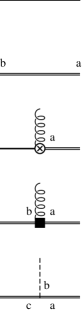
Figure 3: Propagators and vertices of the pNRQCD Lagrangian (at order $1/m^{0}$ and at the NLO in the multipole expansion).

6.2 The $Q\bar{Q}$ potential in perturbation theory

The existence of the different physical scales makes even a purely perturbative definition of the static $Q\bar{Q}$ potential not free from complications. Let us consider the energy of the static quark sources $E_{s}(r)=\displaystyle\lim_{T\to\infty}{i\over T}\ln\langle W_{\Box}\rangle$, (being $W_{\Box}$ the static Wilson loop of size ${\bf r}\times T$, and the symbol $\langle~{}~{}\rangle$ being the average over the gauge fields), which is usually considered as a definition of the static potential. At three loops $E_{s}$ shows infrared divergences[30, 31]. These singularities may indeed be regulated, upon resummation of a certain class of diagrams, which give rise to a sort of dynamical cut-off provided by the difference between the singlet and the octet potential. However, such a dynamical scale is of the same order of the kinetic energy for quarks of large but finite mass and, therefore, should not be included into a proper definition of the static potential in the sense of the Schrödinger equation. This is similar to what happens for the Lamb shift in QED at order $1/m^{2}$. In QCD this effect calls, even in the definition of the static potential, for a rigorous treatment of the bound-state scales. To address the multiscale dynamics of the heavy quark bound state, the concept of effective field theory turns out to be not only helpful but actually necessary.

We answer these questions by performing explicitly the singlet matching at order $1/m^{0}$ and at the NLO in the multipole expansion.

The matching can be done once the interpolating fields for $S$ and $O^{a}$ have been identified in NRQCD. The former need to have the same quantum numbers and the same transformation properties as the latter. The correspondence is not one-to-one. Given an interpolating field in NRQCD, there is an infinite number of combinations of singlet and octet wave-functions with ultrasoft fields, which have the same quantum numbers and, therefore, have a non vanishing overlap with the NRQCD operator. However, the operators in pNRQCD can be organized according to the counting of the multipole expansion. For instance, for the singlet we have

$$\chi^{\dagger}({\bf x}_{2},t)\phi({\bf x}_{2},{\bf x}_{1};t)\psi({\bf x}_{1},t)=Z^{1/2}_{s}(r)S({\bf R},{\bf r},t)+Z^{1/2}_{E,s}(r)r\,{\bf r}\cdot{\bf E}^{a}({\bf R},t)O^{a}({\bf R},{\bf r},t)+\dots,$$ (9)

and for the octet

$$\!\!\!\chi^{\dagger}({\bf x}_{2},t)\phi({\bf x}_{2},{\bf R};t)T^{a}\phi({\bf R},{\bf x}_{1};t)\psi({\bf x}_{1},t) = Z^{1/2}_{o}(r)O^{a}({\bf R},{\bf r},t)$$

$$+ Z^{1/2}_{E,o}(r)r\,{\bf r}\cdot{\bf E}^{a}({\bf R},t)S({\bf R},{\bf r},t)+\dots,$$

$\phi({\bf y},{\bf x};t)\equiv{\rm P}\exp\{ig\int_{0}^{1}\!\!ds\,({\bf y}-{\bf x})\cdot{\bf A}({\bf x}-s({\bf x}-{\bf y}),t)\}$, $Z_{i}$ being normalization factors. These operators guarantee a leading overlap with the singlet and the octet wave-functions respectively. Higher order corrections are suppressed in the multipole expansion. The expressions for the octet can be made manifestly gauge-invariant by inserting a chromomagnetic field in place of the pure color matrix. The fact that the matching can be done in a completely gauge-invariant way enables us to generalize pNRQCD to the case in which $\Lambda_{\rm QCD}\simeq mv$, i.e. to the nonperturbative matching, cf. Sec. 12.

Now, in order to get the singlet potential, we compare 4-quark Green functions. From (9), we take in NRQCD

$$I=\delta^{3}({\bf x}_{1}-{\bf y}_{1})\delta^{3}({\bf x}_{2}-{\bf y}_{2})\langle W_{\Box}\rangle,$$ (11)

and we equate (11) to the singlet propagator in pNRQCD at NLO in the multipole expansion (cf. Fig. 4 for a diagrammatic representation)

$$\!\!\!\!\!\!\!\!\!I=Z_{s}(r)\delta^{3}({\bf x}_{1}-{\bf y}_{1})\delta^{3}({\bf x}_{2}-{\bf y}_{2})e^{-iTV_{s}(r)}\times$$ (12)

$$\!\!\!\!\!\!\!\!\!\!\!\!\Bigg{(}1-{g^{2}\over N_{c}}T_{F}V_{A}^{2}(r)\int_{-T/2}^{T/2}\!\!\!dt\int_{-T/2}^{t}\!\!\!dt^{\prime}e^{-i(t-t^{\prime})(V_{o}-V_{s})}\langle{\bf r}\cdot{\bf E}^{a}(t)\phi(t,t^{\prime})^{\rm adj}_{ab}{\bf r}\cdot{\bf E}^{b}(t^{\prime})\rangle\Bigg{)},$$

where $\phi^{\rm adj}$ is a Schwinger (straight-line) string in the adjoint representation and fields with only temporal argument are evaluated in the centre-of-mass coordinate.

b

Figure 4: The matching between the Wilson loop in NRQCD and the singlet propagator in pNRQCD.

Comparing Eqs. (11) and (12), one gets at the next-to-leading order in the multipole expansion the singlet wave-function normalization $Z_{s}$ and the singlet static potential $V_{s}$. $V_{A}$ and $V_{o}$ must have been previously obtained from the matching of suitable operators, but for the present purposes we only need the tree-level values: $V_{A}=1$ and $V_{o}=(C_{A}/2-C_{F})\alpha_{\rm s}/r$. Let us concentrate here on the matching potential $V_{s}$. By substituting the chromoelectric field correlator in Eq. (12) with its perturbative expression we obtain at the next-to-leading order in the multipole expansion and at order $\alpha_{\rm s}^{4}\ln\alpha_{\rm s}$

$$V_{s}(r)=E_{s}(r)\big{|}_{\rm 2-loop+NNNLL}+C_{F}{\alpha_{\rm s}\over r}{\alpha^{3}_{\rm s}\over\pi}{C_{A}^{3}\over 12}\ln{C_{A}\alpha_{\rm s}\over 2r\mu}.$$ (13)

The 2-loop contribution to $E_{s}$ has been calculated in [25]. The NNNLL contributions arise from the diagrams studied first in [30] and shown below.

b

Note that $V_{s}$ and $E_{s}$ would coincide in QED and that, therefore, this difference here is a genuine QCD feature. Such difference is switched on at NLO in the multipole expansion. An explicit calculation gives [31]

$$\!V_{s}(r)\equiv-C_{F}{\alpha_{V}(r,\mu^{\prime})\over r},\!$$ (14)

$$\!{\alpha}_{V}(r,\mu)=\alpha_{\rm s}(r)\left\{1+\left(a_{1}+2{\gamma_{E}\beta_{0}}\right){\alpha_{\rm s}(r)\over 4\pi}\right.+{\alpha_{\rm s}^{2}(r)\over 16\,\pi^{2}}\bigg{[}\gamma_{E}\left(4a_{1}\beta_{0}+2{\beta_{1}}\right)+\left({\pi^{2}\over 3}+4\gamma_{E}^{2}\right){\beta_{0}^{2}}+a_{2}\bigg{]}\left.\right.$$

$$\left.\quad+{C_{A}^{3}\over 12}{\alpha_{\rm s}^{3}(r)\over\pi}\ln{r\mu^{\prime}}\right\},$$

where $\beta_{n}$ are the coefficients of the beta function ($\alpha_{\rm s}$ is in the $\overline{\rm MS}$ scheme), and $a_{1}$ and $a_{2}$ were given in [25]. We see that the interpretation of the potentials as matching coefficients in pNRQCD implies that the Coulomb potential is not simply coincident with the static energy $E_{s}$. The Coulomb potential turns out to be sensitive to the ultrasoft scale. The same happens with the other potentials (like $V_{o}$ or the potentials that bear corrections in $1/m^{n}$) that can equally be calculated via the matching procedure.

6.3 The singlet potential in the situation $mv\gg\Lambda_{\rm QCD}\gg mv^{2}$

Since in this situation there is a physical scale ($\Lambda_{\rm QCD}$) above the US scale, a potential can be properly defined only once this scale has been integrated out. At the NLO in the multipole expansion we get

$$\!\!\!\!\!\!\!\!\!\!\!\!\!\!\!V_{s}(r)=-C_{F}{\alpha_{V}(r,\mu^{\prime})\over r}-i{g^{2}\over N_{c}}T_{F}V_{A}^{2}(r){r^{2}\over 3}\int_{0}^{\infty}\!\!\!\!dte^{-it(V_{o}-V_{s})}\langle{{\bf E}^{a}}(t)\phi(t,0)^{\rm adj}_{ab}{\bf E}^{b}(0)\rangle(\mu^{\prime}).$$

(15)

Therefore, the heavy quarkonium static potential $V_{s}$ is given in this situation by the sum of the purely perturbative piece calculated in Eq. (14) and a term carrying nonperturbative contributions (contained into non-local gluon field correlators). This last one can be organized as a series of power of $r^{n}$ by expanding $\exp\{-it(V_{o}-V_{s})\}=1-it(V_{o}-V_{s})+\dots$ (since $t\simeq 1/\Lambda_{\rm QCD}$, $V_{o}-V_{s}\simeq mv^{2}$). Typically the nonperturbative piece of Eq. (15) absorbs the $\mu^{\prime}$ dependence of $\alpha_{V}$ so that the resulting potential $V_{s}$ is now scale independent.
We notice that the leading nonperturbative term could be as important as the perturbative potential once the power counting is established and, if so, it should be kept exact when solving the Schrödinger equation. In Table 1 we summarize the different kinematic situations.

b $mv$ $mv^{2}$ potential ultrasoft corrections $\gg\Lambda_{\rm QCD}$ $\gg\Lambda_{\rm QCD}$ perturbative US gluons + local condensates $\gg\Lambda_{\rm QCD}$ $\sim\Lambda_{\rm QCD}$ perturbative US gluons + non-local condensates $\gg\Lambda_{\rm QCD}$ $\ll\Lambda_{\rm QCD}$ perturbative + No US (if light quarks short-range nonpert.     are not considered)

Table 1: Summary of the different kinematic situations.

6.4 The perturbative potential and nonpotential nonperturbative corrections:
Coulombic and quasi-Coulombic systems

Let me define what I mean with Coulombic or quasi-Coulombic systems [37]. If $mv\gg mv^{2}{\ \lower-1.2pt\vbox{\hbox{\hbox to0.0pt{$>$\hss}\lower 6.0pt\vbox{\hbox{$\sim$}}}}\ }\Lambda_{\rm QCD}$, the system is described up to order $\alpha_{\rm s}^{4}$ by a potential which is entirely accessible to perturbative QCD (14). Nonpotential effects start at order $\alpha_{\rm s}^{5}\ln\mu^{\prime}$ [32]. We call Coulombic this kind of system. Nonperturbative effects are of nonpotential type and can be encoded into local (à la Voloshin–Leutwyler[5]) condensates (if $mv^{2}\gg\Lambda_{\rm QCD}$) or non-local condensates (if $mv^{2}\sim\Lambda_{\rm QCD}$): they are suppressed by powers of $\Lambda_{\rm QCD}/mv^{2}$ and $\Lambda_{\rm QCD}/mv$ respectively. We will discuss in details the case of Coulombic systems in the next section.

If $mv\gg\Lambda_{\rm QCD}\gg mv^{2}$, the scale $mv$ can be still integrated out perturbatively, giving rise to the Coulomb-type potential (14). Nonperturbative contributions to the potential arise when integrating out the scale $\Lambda_{\rm QCD}$ [23], precisely as explained in Sec. 6.3. We call quasi-Coulombic the systems where the nonperturbative piece of the potential can be considered small with respect to the Coulombic one and treated as a perturbation.

Some levels of $t\bar{t}$, the lowest level of $b\bar{b}$ may be considered Coulombic systems , while the $J/\psi$, the $\eta_{c}$ and the short-range hybrids may be considered quasi-Coulombic. The $B_{c}$ may be in a boundary situation. As it is typical in an effective theory, only the actual calculation may confirm if the initial assumption about the physical system was appropriate. In Sec. 9 I will give an example of computation in a quasi-Coulombic system after an appropriate redefinition of the mass parameter that subtracts the largest indetermination in the perturbative series.

For all these systems it is relevant to obtain a determination of the energy levels as accurate as possible in perturbation theory.

7 CALCULATION of QUARKONIUM ENERGIES at $O(m\alpha_{s}^{5}\ln\alpha_{s})$

The perturbative energy levels of quarkonium are known at $O(m\alpha_{s}^{4})$[33]. pNRQCD provides us with a well defined way of calculating the energy levels at higher orders, since the size of each term in the pNRQCD Lagrangian is well-defined and since we are now able to calculate the static potential beyond two loops. In order to obtain the leading logs at $O(m\alpha_{\rm s}^{5})$ in the spectrum, $V_{s}$ has to be computed at $O(\alpha_{\rm s}^{4}\ln)$, $V_{s}^{(1)}$ at $O(\alpha_{\rm s}^{3}\ln)$, $V_{s}^{(2)}$ at $O(\alpha_{\rm s}^{2}\ln)$ and $V_{s}^{(3)}$ at $O(\alpha_{\rm s}\ln)$. The matching to pNRQCD at ${\rm N}^{3}$LL accuracy was calculated in [32] and the potentials at the requested accuracy were thus obtained.

The total correction to the energy at $O(m\alpha_{s}^{5}\ln\alpha_{s})$ is given by the sum of the averaged values of the potentials plus the nonpotential contributions,

$$\delta E_{n,l,j}=\delta^{\rm pot}E_{n,l,j}(\mu^{\prime})+\delta^{\rm US}E_{n,l}(\mu^{\prime})\,,$$ (16)

$$\delta E_{n,l,j}^{\rm pot}(\mu^{\prime})=E_{n}{\alpha_{\rm s}^{3}\over\pi}\left\{{C_{A}\over 3}\left[{C_{A}^{2}\over 2}+4C_{A}C_{F}{1\over n(2l+1)}+2C_{F}^{2}\left({8\over n(2l+1)}-{1\over n^{2}}\right)\right]\ln{\mu^{\prime}\over m\alpha_{\rm s}}\right.$$ (17)

$$\quad\quad\quad+{C_{F}^{2}\delta_{l0}\over 3n}\left(8\left[C_{F}-{C_{A}\over 2}\right]\ln{\mu^{\prime}\over m\alpha_{\rm s}}+\left[C_{F}+{17C_{A}\over 2}\right]\ln{\alpha_{\rm s}}\right)\left.\right.$$

$$\quad\quad\quad\left.-{7\over 3}{C_{F}^{2}C_{A}\delta_{l0}\delta_{s1}\over n}\ln{\alpha_{\rm s}}-{(1-\delta_{l0})\delta_{s1}C_{j,l}\over l(2l+1)(l+1)n}{C_{F}^{2}C_{A}\over 2}\ln{\alpha_{\rm s}}\right\},$$

where $E_{n}=-mC_{F}^{2}\alpha_{\rm s}^{2}/(4n^{2})$ and $C_{j,l}=-{(l+1)(4l-1)/(2l-1)}\,{\rm for}\,j=l-1$, $=-1\,{\rm for}\,j=l$ and $={l(4l+5)/(2l+3)}\,{\rm for}\,j=l+1$.

The $\ln\alpha_{\rm s}$ appearing in Eq. (17) come from logs of the type $\ln{1/mr}$ in the potential. Therefore they can be deduced once the dependence on $\ln m$ is known. The $\mu^{\prime}$ dependence of Eq. (17) cancels against contributions from US energies. At the next-to-leading order in the multipole expansion the contribution from these scales reads

$$\delta^{\rm US}E_{n,l}(\mu^{\prime})=-i{g^{2}\over 3N_{c}}T_{F}\times\int_{0}^{\infty}\!\!dt\langle n,l|{\bf r}e^{it(E_{n}-H_{o})}{\bf r}|n,l\rangle\langle{\bf E}^{a}(t)\phi(t,0)^{\rm adj}_{ab}{\bf E}^{b}(0)\rangle(\mu^{\prime}),$$ (18)

where $H_{o}={{\bf p}^{2}/2m}+V_{o}$.

Different possibilities appear depending on the relative size of $\Lambda_{\rm QCD}$ with respect to the US scale $m\alpha_{\rm s}^{2}$. If we consider that $\Lambda_{\rm QCD}\sim m\alpha_{\rm s}^{2}$ the gluonic correlator in Eq. (18) cannot be computed using perturbation theory. We are still able to obtain all the $m\alpha_{s}^{5}\ln({m\alpha_{s}/m})$ and $m\alpha_{s}^{5}\ln({m\alpha_{s}/{\mu^{\prime}}})$ contributions where the ${\mu^{\prime}}$ dependence cancels now against the US contributions that have to be evaluated non-perturbatively.

If we consider that $m\alpha_{\rm s}^{2}\gg\Lambda_{\rm QCD}$, Eq. (18) can be computed perturbatively. Being $m\alpha_{\rm s}^{2}$ the next relevant scale, the effective role of Eq. (18) will be to replace $\mu^{\prime}$ by $m\alpha_{\rm s}^{2}$ (up to finite pieces that we are neglecting) in Eq. (17). Then Eq. (16) simplifies to

$$\delta E_{n,l,j}=E_{n}{\alpha_{\rm s}^{3}\over\pi}\ln{\alpha_{\rm s}}\left\{{C_{A}\over 3}\left[{C_{A}^{2}\over 2}+4C_{A}C_{F}\right.{1\over n(2l+1)}+2C_{F}^{2}\left({8\over n(2l+1)}-{1\over n^{2}}\right)\right]$$

$$\quad+{3C_{F}^{2}\delta_{l0}\over n}\left[C_{F}+{C_{A}\over 2}\right]\left.-{7\over 3}{C_{F}^{2}C_{A}\delta_{l0}\delta_{s1}\over n}-{(1-\delta_{l0})\delta_{s1}\over l(2l+1)(l+1)n}\,C_{j,l}{C_{F}^{2}C_{A}\over 2}\right\}$$ (19)

plus non-perturbative corrections that can be parameterized by local condensates [32, 5] and are of order $\alpha_{s}^{2}({\Lambda_{\rm QCD}\over m\alpha_{s}})^{2}({\Lambda_{\rm QCD}\over m\alpha_{s}^{2}})^{2}$ and higher. For the $\Upsilon(1S)$ and $t\bar{t}$ non-perturbative contributions are expected not to exceed $100\div 150$ MeV and $10$ MeV respectively.

The calculation (19) paves the way to the full ${\rm N}^{3}$LO order analysis of Coulombic systems and is relevant at least for $t\bar{t}$ production and $\Upsilon$ physics. In the first case it is a step forward reaching a 50 MeV sensitivity on the top quark mass for the $t\bar{t}$ cross section near threshold to be measured at future Linear Colliders [43]. In the second case they improve our knowledge of the $b$ mass [33].

In particular, from (19) we can estimate the ${\rm N}^{3}$LL correction to the energy level of the $\Upsilon(1S)$ and we find [32]

$$\delta E_{101}={1730\over 81\pi}m_{b}\alpha_{s}^{4}(\mu)\alpha_{s}(\mu^{\prime})\ln{1/\alpha_{s}(\mu^{\prime})}\simeq(80\div 100)\,{\rm MeV},$$ (20)

which appears not to be small. Corrections from this ${\rm N}^{3}$LL terms have been calculated for the $t\bar{t}$ cross section and $\Upsilon(1S)$ wave function, cf. [35] and [33]. They also turn out to be sizeable.

Large corrections, however, already show up at NLO and ${\rm N}^{2}$LO and are responsible for the bad convergence of the perturbative series in terms of the pole mass.

8 RENORMALONS, the POLE MASS and the PERTURBATIVE EXPANSION

The bad convergence of the perturbative expansion can be, at least in part, attributed to renormalon contributions. The pole mass, thought an infrared safe quantity[39], has long distance contributions of order $\Lambda_{\rm QCD}$[40]. Also the static potential is affected by renormalons (see e.g. [40]). Rephrasing them in the effective field theory language of pNRQCD we can say that the Coulomb potential suffers from IR renormalons ambiguities with the following structure

$$V_{s}(r)|_{\rm IR\,ren}=C_{0}+C_{2}r^{2}+\dots$$ (21)

b

Figure 5: Renormalon in the static potential at LO in the multipole expansion, here $\mu$ is a hard cut-off, $1/r\gg\mu\gg\Lambda_{\rm QCD}$.

b

Figure 6: Renormalon contribution the pole mass.

The constant $C_{0}\sim\Lambda_{\rm QCD}$ is known to be canceled by the IR pole mass renormalon ($2m_{\rm pole}|_{\rm IR\,ren}=-C_{0}$, [40]). Several mass definitions appropriate to explicitly realize this renormalon cancellation have been proposed[41]. Among the others, the $1S$ mass[38] is defined as half of the perturbative contribution to the ${}^{3}S_{1}$ $q\bar{q}$ mass. Unlike the pole mass, the $1S$ mass, containing, by construction, half of the total static energy $\langle 2m+V^{Coul}\rangle$, is free of ambiguities of order $\Lambda_{\rm QCD}$. Taking e.g. the $\Upsilon(1S)$, the $1S$ mass is related to the physical $\Upsilon(1S)$ mass by $E(\Upsilon(1S))=2m_{1S}+\Lambda_{\Upsilon}$. $\Lambda_{\Upsilon}$ is the poorly known non-perturbative contribution, which is likely, as we said, to be less than $100\div 150$ MeV. In the next section we will present an explicit example that shows how, using this mass and thus dealing with quantities that are infrared safe at order $\Lambda_{\rm QCD}$, the pathologies of the perturbative series, due to the renormalon ambiguities affecting the pole mass, are cured.

It is possible to show that the second infrared renormalon, $C_{2}\simeq\Lambda_{\rm QCD}^{3}$, of $V_{s}$ cancels against the appropriate pNRQCD UV renormalon in the contribution to the potential originating at NLO in the multipole expansion. What remains is the explicit expression for the operator which absorbs the $C_{2}\sim\Lambda_{\rm QCD}^{3}$ ambiguity (for details see [23]): such nonperturbative operator turns out to be a nonlocal chromoelectric condensate of the type used in some QCD vacuum models [37, 44].

An interesting open question is if an explicit renormalon subtraction similar to that one at $O(\Lambda_{\rm QCD})$ can be realized at the subsequent order $O(\Lambda_{\rm QCD}^{3})$. This may be relevant since this renormalon is related to the corrections at ${\rm N}^{3}$LL discussed in the previous section. Indeed, it is still an open problem whether the largeness of the ${\rm N}^{3}$LL corrections is an artifact due to our partial knowledge of the contributions at this order, or if it is an artifact due to the fact that the subsequent renormalon cancellation has to be realized at this order or finally if it is a true signal of the breakdown of the perturbative series. To make more definite statements one should know the complete ${\rm N}^{3}$LO or understand the mechanism of cancellation of the second renormalon [42].

In the next section I will present a concrete example of the relevance of the mass renormalon cancellation in order to obtain reliable phenomenological predictions.

9 A QUASI COULOMBIC SYSTEM with
EXPLICIT $O(\Lambda_{\rm QCD})$ RENORMALON CANCELLATION

I consider here the perturbative calculation up to order $m\alpha_{s}^{4}$ of the energy of the $\bar{b}c$ ground state: this will be relevant to a QCD determination of the $B_{c}$ mass if this system is Coulombic or at least quasi-Coulombic. I will assume this to be the case.

In order to calculate the $B_{c}$ mass in perturbation theory up to order $\alpha_{\rm s}^{4}$, we need to consider the following contributions to the potential: the perturbative static potential at two loops, the $1/m$ relativistic corrections at one loop, the spin-independent $1/m^{2}$ relativistic corrections at tree level and the $1/m^{3}$ correction to the kinetic energy. We do not consider $\alpha^{5}_{s}\ln{\alpha_{s}}$ corrections since the mechanism responsible for this large contributions has not yet been understood. Then, we have[46]

$$E(B_{c})_{\rm pert}=m_{b}+m_{c}+E_{0}(\bar{\mu})\left\{\!1\!-{\alpha_{\rm s}(\bar{\mu})\over\pi}\right.\left[\beta_{0}l+{4\over 3}C_{A}-{11\over 6}\beta_{0}\right]+\left({\alpha_{\rm s}\over\pi}\right)^{2}\left[{3\over 4}\beta_{0}^{2}\right.l^{2}+(2C_{A}\beta_{0}$$

$$-{9\over 4}\beta_{0}^{2}-{\beta_{1}\over 4})l-\pi^{2}C_{F}^{2}\left({1\over m_{b}^{2}}+{1\over m_{c}^{2}}-{6\over m_{b}m_{c}}\right)m_{\rm red}^{2}+{5\over 4}\pi^{2}C_{F}^{2}\left({1\over m_{b}^{3}}+{1\over m_{c}^{3}}\right)m_{\rm red}^{3}+\pi^{2}C_{F}C_{A}$$

$$+{4\over 9}C_{A}^{2}-{17\over 9}C_{A}\beta_{0}+\left.\left.\left({181\over 144}+{1\over 2}\zeta(3)+{\pi^{2}\over 24}\right)\beta_{0}^{2}+{\beta_{1}\over 4}+{c\over 8}\right]\right\},$$ (22)

being $m_{\rm red}=m_{b}m_{c}/(m_{b}+m_{c})$, $l=\ln({2C_{F}\alpha_{\rm s}m_{\rm red}/\bar{\mu}})$, $E_{0}(\bar{\mu})=-m_{\rm red}{(C_{F}\alpha_{\rm s}(\bar{\mu}))^{2}/2}$ and $\bar{\mu}$ the scale around which we expand $\alpha_{s}(r)$.

If we use here the pole masses $m_{b}=5$ GeV, $m_{c}=1.8$ GeV and $\bar{\mu}=1.6$ GeV, then we obtain $E(B_{c})_{\rm pert}\simeq 6149$ MeV $\simeq 6800-115-183-353$ MeV, where the second, third and fourth figures are the corrections of order $\alpha_{\rm s}^{2}$, $\alpha_{\rm s}^{3}$ and $\alpha_{\rm s}^{4}$ respectively. The series turns out to be very badly convergent. This reflects also in a strong dependence on the normalization scale $\bar{\mu}$: at $\bar{\mu}=1.2$ GeV we would get $E(B_{c})_{\rm pert}\simeq 5860$ MeV, while at $\bar{\mu}=2.0$ GeV we would get $E(B_{c})_{\rm pert}\simeq 6279$ MeV. The non-convergence of the perturbative series (22) signals the fact that large $\beta_{0}$ contributions (coming from the static potential renormalon) are not summed up and canceled against the pole masses. In order to obtain a well-behaved perturbative expansion, we use, now, the so-called $1S$ mass.

b

Figure 7: $E(B_{c})_{\rm pert}$ as a function of $\bar{\mu}$ at $\Lambda_{\overline{\rm MS}}^{N_{f}=3}=300$ MeV (continuous line). The dashed lines refer to $\Lambda_{\overline{\rm MS}}^{N_{f}=3}=250,350$ MeV respectively.

We consider the perturbative contribution (up to order $\alpha_{s}^{4}$) of the $\,{}^{3}S_{1}$ levels of charmonium and bottomonium:

$$E(J/\psi)_{\rm pert}=f(m_{c});\quad E(\Upsilon(1S))_{\rm pert}=f(m_{b}),$$

which are respectively a function of the $c$ and the $b$ pole mass and can be read off from Eq. (22) in the equal-mass case, adding to it the spin-spin interaction energy: $m(C_{F}\alpha_{\rm s})^{4}/3$. We invert these relations in order to obtain the pole masses as a formal perturbative expansion depending on the $1S$ masses. Finally, we insert the expressions $m_{c}=f^{-1}(E(J/\psi)_{\rm pert})$ and $m_{b}=f^{-1}(E(\Upsilon(1S))_{\rm pert})$ in Eq. (22). At this point we have the perturbative mass of the $B_{c}$ as a function of the $J/\psi$ and $\Upsilon(1S)$ perturbative masses. If we identify the perturbative masses $E(J/\psi)_{\rm pert}$, $E(\Upsilon(1S))_{\rm pert}$ with the physical ones, then the expansion (22) depends only on the scale $\bar{\mu}$. The perturbative series turns out to be reliable for values of $\bar{\mu}$ bigger than $(1.2\div 1.3)$ GeV and lower than $(2.6\div 2.8)$ GeV. For instance, $E(B_{c})_{\rm pert}=6278.5+35+6.5+5.5$ MeV at the scale $\bar{\mu}=1.6$ GeV. Therefore, we obtain now a better convergence of the perturbative expansion and a stable determination of the perturbative mass of the $B_{c}$. This fact seems to support the $B_{c}$ being indeed a Coulombic or quasi-Coulombic system. By varying $\bar{\mu}$ from 1.2 GeV to 2.0 GeV and $\Lambda_{\overline{\rm MS}}^{N_{f}=3}$ from 250 MeV to 350 MeV and by calculating the maximum variation of $E(B_{c})_{\rm pert}$ in the given range of parameters, we get as our final result

$$E(B_{c})_{\rm pert}=6326^{+29}_{-9}\,{\rm MeV}.$$ (23)

As a consequence of the now obtained good behaviour of the perturbative series in the considered range of parameters, the result appears stable with respect to variations of $\bar{\mu}$ (see Fig. 7) and, therefore, reliable from the perturbative point of view. It represents a rather clean prediction of the lowest mass of the $B_{c}$. Notice that all the existing predictions are based either on potential models or on lattice evaluation (with still large errors).

Non-perturbative contributions have not been taken into account so far. They affect the identification of the perturbative masses $E(B_{c})_{\rm pert}$, $E(\Upsilon(1S))_{\rm pert}$, $E(J/\psi)_{\rm pert}$, with the corresponding physical ones through Eq.(22). Let us call these non-perturbative contributions $\Lambda_{B_{c}}$, $\Lambda_{\Upsilon}$ and $\Lambda_{J/\psi}$ respectively. As discussed before, they can be of potential or nonpotential nature. In the latter case they can be encoded into non-local condensates or into local condensates. Non-perturbative contributions affect the identification with the physical $B_{c}$ mass roughly by an amount $\simeq-{\Lambda_{J/\psi}/2}$ $-{\Lambda_{\Upsilon}/2}$ $+\Lambda_{B_{c}}$. Assuming $|\Lambda_{J/\psi}|\leq 300$ MeV, $|\Lambda_{\Upsilon}|\leq 100$ MeV and $\Lambda_{\Upsilon}\leq\Lambda_{B_{c}}\leq\Lambda_{J/\psi}$, the identification of our result (23) with the physical $B_{c}$ mass may, in principle, be affected by uncertainties, due to the unknown non-perturbative contributions, as big as $\pm 200$ MeV. However, the different non-perturbative contributions $\Lambda$ are correlated, so that we expect, indeed, smaller uncertainties. If we assume, for instance, $\Lambda_{\Upsilon}$ and $\Lambda_{J/\psi}$ to have the same sign, which seems to be quite reasonable, then the above uncertainty reduces to $\pm 100$ MeV. This would confirm, indeed, that the effect of the non-perturbative contributions on the result of Eq. (23) is not too large.

10 RENORMALIZATION GROUP IMPROVEMENT
and vNRQCD

Of course the results presented here can be renormalization group improved, i.e. the potentially large logarithms can be resummed. The RG group improvement in pNRQCD has been done only at the level of the static potential [28] up to now. When going beyond the static limit $v=0$ a special care has to be payed to the correct implementation of the renormalization group equations because on the bound state we are dealing with correlated scales $mv$ and $mv^{2}$ [29]. Another EFT, called vNRQCD [26], has been devised explicitly to deal with the resummation of large logs. In this case the treatment is, however, purely perturbative. The Lagrangian is explicitly decomposed in soft, potential and ultrasoft fields:

$$L_{vNRQCD}=L_{s}+L_{p}+L_{u}$$

The matching is performed at the scale $m$. The RG equations evolve simultaneously from the scale $m$ to the correlated scales $mv$ and $mv^{2}$. This seems to provide the correct double logarithms.

The approach of vNRQCD may be complicated by the fact that the different scales remain entangled. Moreover vNRQCD is perturbative by construction and thus cannot be used in order to parameterize nonperturbative effects. The goal of vNRQCD is summing up the logarithms in the velocity. In my opinion, however, the real challenge in heavy quark systems remain the nonperturbative corrections. It is also important to keep in mind that, as I noticed in Sec. 4, the finite part contributions may be as much (or more) relevant as the logarithmic ones.

11 RESULTS and APPLICATIONS

In this Section we just recall a list of physical situations where the presented results of pNRQCD (in the situation of the perturbative matching $mv\gg\Lambda_{\rm QCD}$) have been or may be relevant:

• Toponium cross section [43, 35].

• Determination of the mass of the $b$, once the renormalon contribution has been appropriately subtracted [33, 35, 34].

• Hybrids and gluelumps
  pNRQCD gives model independent predictions on the behaviour of the hybrid static potentials. In particular it predicts for these potentials an octet behaviour at very short distances and it correctly states all the degeneration patterns in the small $r$ region [23, 45]. Moreover, it allows to relate the mass of the gluelumps to the correlation lengths of some nonlocal vacuum field strength correlators [37, 23] allowing us to obtain interesting model independent information on the behaviour of these nonperturbative objects [44].

• Quarkonium scattering, Van Der Waals forces, Quarkonium Production. Work is in progress on these applications.

12 NONPERTURBATIVE MATCHING
pNRQCD for $\Lambda\simeq mv$

In this case the potential interaction is dominated by nonperturbative effects. This is the most interesting situation, in which most of the mesons seem to lie.

A large effort has been made in the last decades in order to obtain from QCD the nonperturbative potentials in the Wilson loop approach. pNRQCD allows us to obtain via a nonperturbative matching all the nonperturbative potentials [47]. On this respect I want to discuss few concepts and results.

In pNRQCD a potential picture for heavy quarkonium emerges at the leading order in the US expansion under the condition that the matching between NRQCD and pNRQCD can be performed within an expansion in $1/m$. The gluonic excitations (hybrids and glueballs) that form a gap of order $\Lambda_{\rm QCD}$ with respect to the quarkonium state can be integrated out and the potentials follow in an unambiguous and systematic way from the nonperturbative matching to pNRQCD. Thus, we recover the quark model from pNRQCD [47]. The US degrees of freedom in this case are not coloured gluons but US gluonic excitations between heavy quarks and pions. They can be systematically included and may eventually affect the leading potential picture. Let us consider for instance the singlet matching potential. Disregarding the US corrections, we have the identification

$$V_{s}(r)=\lim_{T\to\infty}{i\over T}\ln\langle W_{\Box}\rangle.$$

US corrections to this formula are due to pions and US gluonic excitations between heavy quarks, and may be included in the same way as the effects due to US gluons have been included in the perturbative situation.

The complete $1/m^{2}$ potential has been calculated along these lines [47]. There are many appealing and interesting features of this procedure. The matching calculation is performed in the way of the quantum mechanical perturbation theory on the QCD Hamiltonian (where perturbations are counted in orders of $1/m$ and not of $\alpha_{s}$) and only at a later stage the relation with the Wilson loop and field insertions is established. This allows us to have a control on the Fock states of the problem and on the contributions coming from gluonic excitations in the intermediate states. At the end, all the expressions are again given in terms of Wilson loops, which can be evaluated on the lattice or in QCD vacuum models. The potentials turn out to be naturally factorized in a hard part (the matching coefficients at the hard scales inherited by pNRQCD from NRQCD) and a low energy part (the Wilson loops expressions). The power counting may turn out to be quite different from the perturbative (QED-like) situation and this may turn out to be very important for some applications (e.g. quarkonium production).

I will not discuss these very interesting results any longer because it is the content of the review of Antonio Vairo at this Conference [47].

13 CONCLUSION and OUTLOOK

I have shown that it is possible to construct systematically and within a controlled expansion an effective theory of QCD, which describes heavy quark bound states. All known perturbative and nonperturbative regimes (potential, nonpotential), are dynamically present in the theory, which is equivalent to QCD. I have presented many applications of pNRQCD in the situation $\Lambda_{\rm QCD}\ll mv$. In the situation $\Lambda_{\rm QCD}\simeq mv$, I have shortly discussed how pNRQCD allows us to systematically factorize the nonperturbative heavy quark dynamics. Similar techniques have been applied to pionium [48]. Acknowledgements

I thank the Organizers, especially Vladimir Petrov and Sergei Klishevich, for arranging such an interesting and nice Conference and for providing the participants with a particularly warm hospitality, a friendly and enjoable atmosphere and a perfect organization. I wish that this series of Conferences could continue like this in the future.

I thank Antonio Vairo for reading the manuscript and for useful comments.

References

- [1] T. Kinoshita, Singapore: World Scientific (1990) 997 p. (Advanced series on directions in high energy physics, 7).
- [2] A. Vairo, Found. Phys. 28, 829 (1998) [hep-ph/9807458].
- [3] C. D. Roberts and A. G. Williams, Prog. Part. Nucl. Phys. 33, 477 (1994) [hep-ph/9403224]; C. D. Roberts and S. M. Schmidt, Prog. Part. Nucl. Phys. 45S1, 1 (2000) [nucl-th/0005064].
- [4] N. Brambilla and A. Vairo, in Lectures given at the 13th Annual HUGS at CEBAF (HUGS 98) in Newport News 1998, Strong interactions at low and intermediate energies pags. 151-220. [hep-ph/9904330]; G. S. Bali, hep-ph/0001312; F. J. Yndurain, hep-ph/9910399.
- [5] M. B. Voloshin, Nucl. Phys. B154, 365 (1979); H. Leutwyler, Phys. Lett. B98, 447 (1981).
- [6] N. Isgur and M. B. Wise, Phys. Lett. B237, 527 (1990); M. Neubert, hep-ph/9610266; B. Grinstein, hep-ph/9508227.
- [7] B. Grinstein, Nucl. Phys. B339, 253 (1990).
- [8] T. Mannel, W. Roberts and Z. Ryzak, Nucl. Phys. B368, 204 (1992).
- [9] S. Balk, J. G. Korner and D. Pirjol, Nucl. Phys. B428, 499 (1994) [hep-ph/9307230].
- [10] W. E. Caswell and G. P. Lepage, Phys. Lett. B167, 437 (1986). G. T. Bodwin, E. Braaten and G. P. Lepage, Phys. Rev. D51, 1125 (1995) [hep-ph/9407339].
- [11] A. V. Manohar, Phys. Rev. D56, 230 (1997) [hep-ph/9701294].
- [12] B. Grinstein, Int. J. Mod. Phys. A15, 461 (2000) [hep-ph/9811264]; I. Z. Rothstein, hep-ph/9911276.
- [13] A. Pineda and J. Soto, Phys. Rev. D58, 114011 (1998) [hep-ph/9802365].
- [14] G. Amoros, M. Beneke and M. Neubert, Phys. Lett. B401, 81 (1997) [hep-ph/9701375].
- [15] C. Bauer and A. V. Manohar, Phys. Rev. D57, 337 (1998) [hep-ph/9708306].
- [16] M. Finkemeier, H. Georgi and M. McIrvin, Phys. Rev. D55, 6933 (1997) [hep-ph/9701243]; M. Luke and A. V. Manohar, Phys. Lett. B286, 348 (1992) [hep-ph/9205228]. Y. Chen and Y. Kuang, Z. Phys. C67, 627 (1995) [hep-ph/9312209].
- [17] Y. Chen, Y. Kuang and R. J. Oakes, Phys. Rev. D52, 264 (1995) [hep-ph/9406287]; N. Brambilla and A. Vairo, Nucl. Phys. Proc. Suppl. 74, 201 (1999) [hep-ph/9809230]; N. Brambilla and A. Vairo, Fizika B8, 261 (1999) [hep-ph/9902360].
- [18] B. A. Thacker and G. P. Lepage, Phys. Rev. D43, 196 (1991); C. T. Davies, K. Hornbostel, G. P. Lepage, A. Lidsey, P. McCallum, J. Shigemitsu and J. H. Sloan [UKQCD Collaboration], Phys. Rev. D58, 054505 (1998) [hep-lat/9802024].
- [19] G. P. Lepage, L. Magnea, C. Nakhleh, U. Magnea and K. Hornbostel, Phys. Rev. D46, 4052 (1992) [hep-lat/9205007].
- [20] A. Vairo, hep-ph/9809229.
- [21] A. Pineda and J. Soto, Nucl. Phys. Proc. Suppl. 64, 428 (1998) [hep-ph/9707481].
- [22] P. Labelle, Phys. Rev. D58, 093013 (1998) [hep-ph/9608491]; H. W. Griesshammer, Phys. Rev. D58, 094027 (1998) [hep-ph/9712467]. M. Beneke, A. Signer and V. A. Smirnov, Phys. Lett. B454, 137 (1999) [hep-ph/9903260]; B. Grinstein and I. Z. Rothstein, Phys. Rev. D57, 78 (1998) [hep-ph/9703298]; A. Pineda and J. Soto, Phys. Rev. D59, 016005 (1999) [hep-ph/9805424].
- [23] N. Brambilla, A. Pineda, J. Soto and A. Vairo, Nucl. Phys. B566, 275 (2000) [hep-ph/9907240];
- [24] A. Vairo, hep-ph/0010191. N. Brambilla, hep-ph/0008279.
- [25] Y. Schroder, Phys. Lett. B447, 321 (1999) [hep-ph/9812205]; M. Peter, Phys. Rev. Lett. 78, 602 (1997) [hep-ph/9610209]; A. Billoire, Phys. Lett. B92, 343 (1980).
- [26] A. V. Manohar and I. W. Stewart, hep-ph/0003107; M. E. Luke, A. V. Manohar and I. Z. Rothstein, Phys. Rev. D61, 074025 (2000) [hep-ph/9910209].
- [27] A. Barchielli et al. Nuovo Cim. A103, 59 (1990); D. Gromes, Z. Phys. C26, 401 (1984).
- [28] A. Pineda and J. Soto, hep-ph/0007197.
- [29] A. V. Manohar, J. Soto and I. W. Stewart, Phys. Lett. B486, 400 (2000) [hep-ph/0006096].
- [30] T. Appelquist, M. Dine and I. J. Muzinich, Phys. Rev. D17, 2074 (1978); L. S. Brown and W. I. Weisberger, Phys. Rev. D20, 3239 (1979).
- [31] N. Brambilla, A. Pineda, J. Soto and A. Vairo, Phys. Rev. D60, 091502 (1999) [hep-ph/9903355].
- [32] N. Brambilla, A. Pineda, J. Soto and A. Vairo, Phys. Lett. B470, 215 (1999) [hep-ph/9910238]; B. A. Kniehl and A. A. Penin, Nucl. Phys. B563, 200 (1999) [hep-ph/9907489].
- [33] F. J. Yndurain, hep-ph/0008007; F. J. Yndurain, hep-ph/0002237.
- [34] A. H. Hoang, hep-ph/0008102.
- [35] B. A. Kniehl and A. A. Penin, Nucl. Phys. B577, 197 (2000) [hep-ph/9911414].
- [36] N. Brambilla, hep-ph/0009143.
- [37] N. Brambilla and A. Vairo, hep-ph/0004192.
- [38] A. H. Hoang, Z. Ligeti and A. V. Manohar, Phys. Rev. Lett. 82, 277 (1999) [hep-ph/9809423].
- [39] A. S. Kronfeld, Phys. Rev. D58, 051501 (1998) [hep-ph/9805215].
- [40] M. Beneke, Phys. Lett. B434, 115 (1998) [hep-ph/9804241]. A. H. Hoang, M. C. Smith, T. Stelzer and S. Willenbrock, Phys. Rev. D59, 114014 (1999) [hep-ph/9804227].
- [41] A. H. Hoang and T. Teubner, Phys. Rev. D60, 114027 (1999) [hep-ph/9904468]; I. Bigi, M. Shifman and N. Uraltsev, Ann. Rev. Nucl. Part. Sci. 47, 591 (1997) [hep-ph/9703290]; O. Yakovlev and S. Groote, hep-ph/0009014.
- [42] Y. Kiyo and Y. Sumino, hep-ph/0007251; Y. Sumino, hep-ph/0004087.
- [43] A. H. Hoang et al., Eur. Phys. J. direct C3, 1 (2000) [hep-ph/0001286].
- [44] H. G. Dosch et al., Phys. Lett. B452, 379 (1999) M. Baker et al. Phys. Rev. D58, 034010 (1998); H. G. Dosch, Phys. Lett. B190, 177 (1987).
- [45] N. Brambilla, Nucl. Phys. Proc. Suppl. 86, 389 (2000) [hep-ph/9909211].
- [46] N. Brambilla and A. Vairo, Phys. Rev. D62, 094019 (2000) [hep-ph/0002075].
- [47] A. Vairo, contribution to this conference hep-ph/0009146; see also N. Brambilla, A. Pineda, J. Soto and A. Vairo, hep-ph/0002250; A. Pineda and A. Vairo, hep-ph/0009145; N. Brambilla and A. Vairo, Phys. Rev. D55, 3974 (1997) [hep-ph/9606344]; N. Brambilla, in Proceedings of Quark Confinement and the Hadron spectrum III, Ed. N. Isgur, World Scientific 2000, pags. 37-56. [hep-ph/9809263].
- [48] D. Eiras and J. Soto, Phys. Rev. D61, 114027 (2000) [hep-ph/9905543]; J. Gasser, V. E. Lyubovitskij and A. Rusetsky, hep-ph/9910524; H. Sazdjian, Phys. Lett. B490, 203 (2000) [hep-ph/0004226]; V. Antonelli, A. Gall, J. Gasser and A. Rusetsky, hep-ph/0003118.