University of Wisconsin - Madison MADPH-00-1199 FERMILAB-Pub-00/318-T AMES-HET-00-12 hep-ph/0012017 November 2000
Exploring Neutrino Oscillations with Superbeams
V. Barger1, S. Geer2, R. Raja2, and K. Whisnant3
1Department of Physics, University of Wisconsin,
Madison, WI 53706, USA
2Fermi National Accelerator Laboratory, P.O. Box 500,
Batavia, IL 60510, USA
3Department of Physics and Astronomy, Iowa State University,
Ames, IA 50011, USA
Abstract
We consider the medium- and long-baseline oscillation physics capabilities of intense muon-neutrino and muon-antineutrino beams produced using future upgraded megawatt-scale high-energy proton beams. In particular we consider the potential of these conventional neutrino “superbeams” for observing oscillations, determining the hierarchy of neutrino mass eigenstates, and measuring -violation in the lepton sector. The physics capabilities of superbeams are explored as a function of the beam energy, baseline, and the detector parameters (fiducial mass, background rates, and systematic uncertainties on the backgrounds). The trade-offs between very large detectors with poor background rejection and smaller detectors with excellent background rejection are illustrated. We find that, with an aggressive set of detector parameters, it may be possible to observe oscillations with a superbeam provided that the amplitude parameter is larger than a few . If is of order or larger, then the neutrino mass hierarchy can be determined in long-baseline experiments, and if in addition the large mixing angle MSW solution describes the solar neutrino deficit then there is a small region of parameter space within which maximal -violation in the lepton sector would be observable (with a significance of a few standard deviations) in a low-energy medium-baseline experiment. We illustrate our results by explicitly considering massive water Cherenkov and liquid argon detectors at superbeams with neutrino energies ranging from 1 GeV to 15 GeV, and baselines ranging from 295 km to 9300 km. Finally, we compare the oscillation physics prospects at superbeams with the corresponding prospects at neutrino factories. The sensitivity at a neutrino factory to violation and the neutrino mass hierarchy extends to values of the amplitude parameter that are one to two orders of magnitude lower than at a superbeam.
I Introduction
Measurements [1, 2] of the neutrino flux produced by cosmic ray interactions in the atmosphere [3] have led to a major breakthrough in our understanding of the fundamental properties of neutrinos. The early observations of the atmospheric neutrino interaction rates found a muon-to-electron event ratio of about 0.6 times the expected ratio. This anomaly was interpreted[4] as evidence for neutrino oscillations with large amplitude and neutrino mass-squared difference eV2. Continued experimental studies[1, 2], especially by the SuperKamiokande (SuperK) collaboration, have firmly established that the deviation of the ratio from expectation is due to a deficit of muon events. This muon deficit increases with zenith angle, and hence with path length, and is consistent with expectations for muon-neutrino oscillations to some other neutrino flavor or flavors with maximal or near-maximal amplitude and eV2. In principle could be (electron-neutrino), (tau-neutrino), or (sterile neutrino) [5]. However, the observed flux is in approximate agreement with the predicted flux for all zenith angles[1], which rules out oscillations with large amplitude. The null results from the CHOOZ and Palo Verde reactor disappearance experiments[6] also exclude oscillations at a mass-squared-difference scale eV2 with amplitude . Furthermore, large amplitude oscillations at the scale are also excluded by SuperK. This is because oscillations are expected to be significantly affected by propagation through matter [7, 8], causing a distortion in the zenith-angle distribution at large angles (corresponding to long path lengths) that is not present in the data [9]. The zenith-angle distribution observed by SuperK excludes oscillations of maximal amplitude at 99% confidence level[9]. We conclude that, if the oscillation interpretation of the atmospheric neutrino deficit is correct, the dominant mode must be oscillation, with the possibility of some smaller amplitude muon-neutrino oscillations to sterile and/or electron-neutrinos[10].
An exotic alternative interpretation[11] of the atmospheric neutrino disappearance results is that a neutrino mass-eigenstate, which is a dominant component of the state, decays to a lighter mass-eigenstate and a Majoron[12]. The first oscillation minimum in must be observed or excluded to differentiate neutrino oscillations from neutrino decays. Unfortunately, the SuperK neutrino-energy and angular-resolution functions smear out the characteristic event rate dip that would correspond to the first oscillation minimum, which cannot therefore be resolved.
Progress in establishing neutrino oscillations at the atmospheric scale is expected in the near future at accelerator neutrino sources with detectors at medium to long baselines. The K2K experiment, from KEK to SuperK[13], with a baseline km and average neutrino energy GeV, is underway. Their preliminary results are in excellent agreement with the oscillation expectations (27 events are observed, whereas 27 events would be expected with oscillations and 40 events for no oscillations[13]). The MINOS experiment from Fermilab to Soudan [14] with km and GeV, which begins operation in 2003, is expected to resolve the first oscillation minimum in and to search for oscillations at the scale with an amplitude sensitivity of . Beginning in 2005, similar physics measurements will be made by the ICARUS[15] and OPERA[16] experiments with neutrinos of average energy GeV from CERN detected at km in the Gran Sasso laboratory.
In addition to the atmospheric neutrino deficit, there are other possible indications of neutrino oscillations. In particular, the long-standing deficit of solar neutrinos [17, 18, 19, 20] compared to the Standard Solar Model (SSM) predictions [21] is widely interpreted as an oscillation depletion of the flux. Note that helioseismology and other solar observations stringently limit uncertainties in the central temperature of the sun and other solar model parameters[22]. The deficit relative to prediction is about one-half for the water Cherenkov [18, 19] and Gallium experiments [20], with the Chlorine experiment [17] finding a suppression of about one-third. The latest solar neutrino results from SuperK show an electron recoil spectrum that is flat in energy, and exhibits no significant day-night or seasonal variation [23].
An industry has developed to extract the allowed ranges of and mixing angles that can account for the solar neutrino data. The analyses take account of the coherent scattering of on matter [7], both in the Sun (the MSW effect [24]) and in the Earth [25]. These matter effects can make significant modifications to vacuum oscillation amplitudes. Until recently, four viable regions of the parameter space were found in global fits to the data:
-
(i)
LMA — large mixing angle with small matter effects ( to );
-
(ii)
SMA — small mixing angle with large matter effects ();
-
(iii)
LOW — large-angle mixing with quasi-vacuum amplitude ();
-
(iv)
VO — large-angle vacuum mixing with small matter effects ().
The latest global solar neutrino analysis by the SuperK collaboration[23] strongly favors solar oscillations to active neutrinos ( and/or ) in the LMA region. A very small area in the LOW region is also allowed at 99% C.L., while the SMA and VO regions are rejected at 95% C.L. However, other global analyses disagree that the latter regions are excluded [26]. Moreover, solar oscillations may also still be viable[27, 28]. The relative weighting of different experiments (e.g. inclusion or exclusion of the Cl data) and whether the 8B flux is held fixed at its SSM value or allowed to float in the global fits presumably account in part for the differences in conclusions. It is expected that the KamLAND reactor experiment [29] will be able to measure to % accuracy and to accuracy [30] if the LMA solar solution is correct.
Finally, the LSND accelerator experiment[31] reports evidence for possible and oscillations with very small amplitude and . If, in addition to the LSND observations, the atmospheric and solar effects are also to be explained by oscillations, then three distinct scales are needed, requiring a sterile neutrino in addition to the three active neutrino flavors[5, 10, 27, 28]. The MiniBooNE experiment at Fermilab[32] is designed to cover the full region of oscillation parameters indicated by LSND.
The principal goals of our analyses are to examine the relative merits of different neutrino “superbeam” scenarios, where we define a neutrino superbeam as a conventional neutrino beam generated by decays, but using a very intense megawatt(MW)-scale proton source. In particular, we are interested in the physics reach in medium- and long-baseline experiments with a neutrino superbeam, and how this reach depends upon the beam energy, baseline, and the parameters of the neutrino detector. As representative examples we explicitly consider water Cherenkov, liquid argon and iron scintillator detectors. However, we note that there is room for new detector ideas, detector optimization, and possibly an associated detector R&D program. Therefore, results are presented that apply to any detector for which the effective fiducial mass and background rates can be specified. Finally, we will discuss the role that neutrino superbeams might play [33, 34] en route to a neutrino factory [35, 36]. Our calculations are performed within a three-neutrino oscillation framework with the parameters chosen to describe the atmospheric neutrino deficit and the solar neutrino deficit assuming the LMA solution. However, our considerations for long-baseline experiments are relevant even if there are additional short-baseline oscillation effects associated with a fourth neutrino [37].
The central objective of long-baseline neutrino oscillation experiments is to determine the parameters of the neutrino mixing matrix and the magnitudes and signs of the neutrino mass-squared differences; the signs fix the hierarchy of the neutrino mass eigenstates [38]. For three neutrinos the mixing matrix relevant to oscillation phenomena can be specified by three angles and a phase associated with -violation [see Eq. (10) below]. There are only two independent mass-squared differences (e.g. and ) for three neutrinos. The muon-disappearance measurements at SuperK constrain and . The other parameter that enters at the leading oscillation scale is , and its measurement requires the observation of neutrino appearance in , , or oscillations.
In long-baseline experiments, if is nonzero, matter effects [7, 39, 40] modify the probability for oscillations involving a or in a way that can be used to determine the sign of [38, 41, 42, 43]. Matter effects give apparent -violation, but this may be disentangled from intrinsic -violation effects [38, 44, 45, 46, 47, 48, 49, 50, 51, 52] at optimally chosen baselines. Matter can also modify the effects of intrinsic or violation [53]. Intrinsic violation may also be studied at short baselines where matter effects are relatively small [54, 55]. -violating effects enter only for values of where oscillations associated with the subleading become significant [56, 57]. The most challenging goal of accelerator-based neutrino oscillation experiments is to detect, or place stringent limits on, violation in the lepton sector. We will address the extent to which this may be possible with conventional superbeams.
II Three-Neutrino Formalism
The flavor eigenstates are related to the mass eigenstates in vacuum by
| (1) |
where is a unitary mixing matrix. The propagation of neutrinos through matter is described by the evolution equation [7, 58]
| (2) |
where and is the amplitude for coherent forward charged-current scattering on electrons,
| (3) |
where is the electron fraction and is the matter density. In the Earth’s crust the average density is typically 3–4 gm/cm3 and . The propagation equations can be re-expressed in terms of mass-squared differences:
| (4) |
where . We assume , and that the sign of can be either positive or negative, corresponding to the case where the most widely separated mass eignstate is either above or below, respectively, the other two mass eigenstates. Thus the sign of determines the ordering of the neutrino masses. The evolution equations can be solved numerically taking into account the dependence of the density on depth using the density profile from the preliminary reference earth model[59]. We integrate the equations numerically along the neutrino path using a Runge-Kutta method. The step size at each point along the path is taken to be 1% of the shortest oscillation wavelength given by the two scales and .
It is instructive to examine analytic expressions for the vacuum probabilities. We introduce the notation
| (5) |
The vacuum probabilities are then given by
| (7) | |||||
where is the -violating invariant[60, 61],
| (8) |
and is the associated dependence on and ,
| (9) |
The mixing matrix can be specified by 3 mixing angles () and a -violating phase (). We adopt the parameterization
| (10) |
where and . We can restrict the angles to the first quadrant, , with in the range . In this parameterization is given by
| (11) |
For convenience we also define
| (12) |
Then the vacuum appearance probabilities are given by
| (14) | |||||
| (18) | |||||
| (20) | |||||
The corresponding probabilities can be obtained by reversing the sign of in the above formulas (only the term changes sign in each case). The probabilities for are the same as those for , assuming invariance. Tests of non-invariance are important [62, 63, 64] but beyond the scope of the present analysis. The are not independent, and can be expressed in terms of and . Then and
| (21) | |||||
| (22) |
Since Eqs. (14)–(22) in their exact form are somewhat impenetrable, we make a few simplifying assumptions to illustrate their typical consequences. First, it is advantageous in long-baseline experiments to operate at an value such that the leading oscillation is nearly maximal, i.e. . Since , and to a good approximation we can ignore terms involving . Also, since is already constrained by experiment to be small, for the terms involving we retain only the leading terms in . Second, at the value for which the leading oscillation is best measured, . Even if is not close to for all neutrino energies in the beam, an averaging over the energy spectrum will suppress if the neutrinos at the middle of the spectrum have . With the above approximations the vacuum oscillation probabilities simplify to
| (23) | |||||
| (24) | |||||
| (25) |
It is interesting to compare the relative sizes of the leading -violating () and -conserving () terms in the oscillation probability:
| (26) |
For the standard three-neutrino solution to the solar and atmospheric data with large-angle mixing in the solar sector, the first fraction on the right-hand side of Eq. (26) is of order unity, and the relative size of the term is
| (27) |
As an example, with eV2 and km/GeV, ; then with and (its maximum allowed value), the term is about 25% of the term. Smaller values of or decrease the ratio in Eq. (27); smaller values of increase it.
While smaller values of give a larger relative term, they will also reduce the overall event rate since the term is proportional to . The effect may be hard to measure if the event rate is low (due to insufficient flux or a small detector). Because the number of events is proportional to , the statistical uncertainty on the event rate is proportional to for small and Gaussian statistics. Since the number of events is also proportional to , the size of the signal relative to the statistical uncertainties does not decrease as becomes smaller. Therefore, a priori it does not follow that small automatically makes undetectable [65].
On the other hand, even if the event rate is high enough to overcome the statistical uncertainties on the signal, backgrounds will limit the ability to measure . Background considerations place an effective lower bound on the values of for which a search can be made. This can be quantified by noting that the ratio of the number of events to the uncertainty due to the background is (assuming Gaussian statistics), where is the number of events without oscillations and is the background fraction. can be expressed as the part of the oscillation probability times . Using the expression for the probability in Eq. (23), it follows that a effect in the channel requires
| (28) |
For and , a typical experiment with and can detect for . The detailed calculations in Sec. V confirm this approximate result.
The preceding discussion applies only when the corrections due to matter are not large, generally when is small compared to the Earth’s radius. Reference [54] gives approximate expressions for the probabilities when the matter corrections are small but not negligible. However, the most striking matter effects occur when the matter corrections are large and the expansions of Ref. [54] are no longer valid (see, e.g., the plots of oscillation probabilities in matter given in Ref. [66]).
Some of the qualitative properties of neutrino oscillations in matter can be determined by considering only the leading oscillation and assuming a constant density. There is an effective mixing angle in matter defined by
| (29) |
where is given in Eq. (3). The oscillation probabilities in the leading oscillation approximation for constant density are [41, 67]
| (30) | |||||
| (31) | |||||
| (32) |
where the oscillation arguments are
| (33) |
and
| (34) |
The term in must be retained here because it is not necessarily negligible compared to , due to matter effects. The expressions for antineutrinos may be generated by changing the sign of .
In Eq. (29) there is a resonant enhancement of oscillations when ( for antineutrinos). This occurs for neutrinos when and for antineutrinos when . On resonance, there is a suppression for antineutrinos (neutrinos) when (). This enhancement of one channel and suppression of the other then gives a fake violation due to matter effects.
In the event that the contribution of the sub-leading oscillation is not negligible, the true effects due to also enter, but they may be masked by matter effects. Numerical calculations [42] show that for distances larger than 2000 km matter effects dominate the true for and vice versa for .
As long as is not too small, one approach is to have large enough so that the dominant effect is from matter and the sign of is clearly determinable; then the true effect can be extracted by considering deviations from the -conserving predictions [42]. With large , the neutrino energies must be high enough that (e.g., km requires GeV). An alternative approach is to have short where the matter effects are relatively small [54]; this usually requires a smaller to have of order (e.g., km and GeV). We will study both of these possibilities in this paper.
For , the matter effect is similar in size or smaller than the true effect, and it may not be possible to distinguish between large intrinsic with very small from no intrinsic with a moderate-sized . Even in experiments at short distances (where the matter effect is small) the number of appearance events may be too small relative to the background to have a statistically significant difference between the neutrino and antineutrino oscillation probabilities. The existence of intrinsic violation may be very difficult to determine in this case.
III Conventional neutrino beams
Conventional neutrino beams are produced using a pion decay channel. If the pions are charge-sign selected so that only positive (negative) particles are within the channel, the pion decays () will produce a beam of muon neutrinos (antineutrinos). The beams will also contain small components of and from kaon and muon decays. For a positive beam, the dominant decays that contribute to the component are and . If the pion beam has not been charge-sign selected there will also be a contribution from decays. The “contamination” can be minimized using beam optics that disfavor decays occurring close to the target [note: ], and choosing a short decay channel to reduce the contribution from muon decays. These strategies enhance the flavor purity of the beam, but reduce the beam flux. Depending on the beamline design, the resulting contamination is typically at the few parts in 100 to a few parts in 1000 level. The intrinsic component in the beam produces a background that must be subtracted in a oscillation search. Ultimately, the systematic uncertainty associated with the background subtraction will degrade the sensitivity of the oscillation measurement.
To maximize the neutrino flux in the forward direction it is desirable that the pion beam divergence is small within the decay channel. The required radial focusing can be provided by a quadrupole channel and/or magnetic horns. The beamline optics (dipoles, horns, and quadrupoles) determine the peak pion energy and energy spread within the decay channel, and hence determine the neutrino spectrum. If the optics are designed to accept a large pion momentum spread the resulting wide band beam (WBB) will contain a large neutrino flux with a broad energy spectrum. If the optics are designed to accept a smaller pion momentum spread, the resulting narrow band beam (NBB) will have a narrower energy spread, but a smaller flux.
A Detectors and backgrounds
We are primarily interested in searching for, and measuring, and oscillations. The experimental signature for these oscillation modes is the appearance of an energetic electron or positron in a charged-current (CC) event. The electron must be separated from the hadronic remnants produced by the fragmenting nucleon. Backgrounds can arise from (i) energetic neutral pions that are produced in neutral-current (NC) interactions, and subsequently fake a prompt-electron signature, (ii) energetic neutral pions that are produced in CC interactions in which the muon is undetected, and the fakes an electron, (iii) charm production and semileptonic decay, (iv) oscillations followed by decay of the tau-lepton to an electron. Backgrounds (iii) and (iv) can be suppressed using a low-energy neutrino beam.
Background (i) is potentially the most dangerous since leading production in NC events is not uncommon. Indeed, in a recent study [68, 69] using a low energy beam it has been shown that in a water Cherenkov detector (e.g. SuperK) it is difficult to reduce this background to a level below (3%) of the CC rate. A liquid argon detector is believed to provide much better -electron discrimination, and will perhaps enable the background to be reduced to (0.1%) of the CC rate [70]. Based on these considerations there are two different detector strategies. We can choose a water Cherenkov detector, enabling us to maximize the detector mass, and hence the event statistics, but obliging us to tolerate a significant background from production in NC events. Alternatively, we can choose a detector technology that highly suppresses the background, but this will oblige us to use a smaller fiducial mass, and hence lower event statistics.
For a given choice of beamline design, baseline, and detector parameters, the experimental and sensitivities can be calculated. It is useful to define some representative scenarios, characterized by (a) the parameters of the primary proton beam incident on the pion production target, (b) the data sample size (kt-years), defined as the product of the detector fiducial mass, the efficiency of the signal selection requirements, and the number of years of data taking, (c) the background fraction defined as the background rate divided by the CC rate for events that survive the signal selection requirements, and (d) the fractional systematic uncertainty on the predicted .
We will consider neutrino superbeams that can be produced with MW-scale proton beams at low energy ( GeV) at the proposed Japan Hadron Facility (JHF) and at high energy ( GeV) at laboratories with high-energy proton drivers that might be upgraded to produce these superbeams (BNL, CERN, DESY, and Fermilab). For the sake of definiteness, in the following we will restrict our considerations to two explicit MW-scale primary proton beams. First, we will consider the 0.77 MW beam at the 50 GeV proton synchrotron of the proposed JHF, and a 4 MW upgrade which we refer to as SJHF (Superbeam JHF). Second, we consider a 1.6 MW proton driver upgrade that is under study at Fermilab. With this new proton driver, and modest upgrades to the 120 GeV Fermilab Main Injector (MI), it is possible to increase the beam current within the MI by a factor of four, and hence increase the intensity of the NuMI beam by a factor of four, which we refer to as SNuMI (Superbeam NuMI). Higher beam intensities are precluded by space-charge limitations in the MI [71]. For both the SJHF and SNuMI cases we will assume a run plan in which there is 3 years of data taking with a neutrino beam followed by 6 years of data taking with an antineutrino beam. In principle the high-energy superbeams could be produced at any of the present laboratories with high-energy proton drivers.
We define three aggressive detector scenarios, which are summarized in Table I:
-
Scenario , which might be realized with a liquid argon detector. We choose a 30 kt fiducial mass, which has been considered previously for a neutrino factory detector. We assume tight selection requirements are used to suppress the background, and take the signal efficiency to be 0.5. This will result in kt-years for neutrino running and kt-years for antineutrino running. We assume that backgrounds from events contribute 0.001 to [72], and the contamination in the beam contributes 0.003 to in neutrino running, and to in antineutrino running. We neglect all other backgrounds. Hence, (0.006) for neutrino (antineutrino) running. Finally, we will assume that we know the background rate with a precision of 10% ().
-
Scenario , which might be realized with a fine-grain iron sampling calorimeter. We choose a 10 kt fiducial mass, which is a factor of 10 larger than the THESEUS detector [73]. Since this fiducial mass is smaller than for the alternative scenarios we are considering, we will assume that the selection cuts are not tight, and that the selection efficiency is 0.9. This will result in kt-years for neutrino running and kt-years for antineutrino running. We assume that backgrounds from events contribute 0.01 to , and the contamination in the beam contributes 0.003 to in neutrino running, and to in antineutrino running. We neglect all other backgrounds. Hence, (0.015) for neutrino (antineutrino) running. Finally, we will assume that we know the background rate with a precision of 10% ().
-
Scenario , which might be realized for a low-energy beam with a water Cherenkov detector. We choose a 220 kt fiducial mass, a factor of 10 larger than the SuperK detector. Guided by the study described in Ref. [68] we will assume the selection requirements used to suppress the background result in a signal efficiency of 0.68. This will result in kt-years for neutrino running and kt-years for antineutrino running. We assume that backgrounds from events dominate, and set . Note that a detailed detector simulation has obtained for a water Cherenkov detector at a low energy NBB at the JHF [68]. With further optimization the choice might therefore be realizable at low energy, but for higher energy ( GeV) neutrino beams the rejection against the background is expected to be much worse. Hence, a new detector technology might be required for this scenario to make sense at high energies. Finally, we will assume that we know the background rate with a precision of 10% ().
Scenarios , , and are very aggressive, and may or may not be realizable in practice. In the following we will explore the oscillation sensitivity as a function of , , , baseline, and neutrino beam energy. Scenario is clearly inferior to scenario , which has larger and smaller . Therefore, in the following we will not discuss the scenario physics potential in detail, but we will indicate the scenario physics potential on several relevant figures. We will use scenarios and extensively to illustrate the physics potential of upgraded conventional neutrino beams, and facilitate a discussion of the challenges involved in probing small values of .
IV reach
For a given neutrino beam, baseline, and detector, we wish to calculate the resulting reach, which we define as the value of that would result in a or signal that is 3 standard deviations above the background. In our analysis we will take into account the Poisson statistical uncertainties on the numbers of signal and background events, and the systematic uncertainty on the background subtraction. Our prescription for determining the reach is given in the appendix. In the following, unless otherwise stated, the reaches are calculated setting the sub–leading oscillation parameters and eV2. The small effectively switches off contributions from the sub–leading scale. Larger values of can yield contributions to the signal, but these contributions are not important unless is significantly less than .
A Sensitivity at the Japan Hadron Facility
The Japan Hadron Facility working group has recently investigated [68] the oscillation sensitivity attainable at the proposed 0.77 MW 50 GeV proton synchrotron in Japan, using a 295 km baseline together with the SuperK detector. In their study they considered a variety of low energy ( GeV) WBB and NBB beamline designs. The resulting experimental scenario is similar to the one later considered in Ref. [33]. The conclusions from the study were: (i) With a water Cherenkov detector the sensitivity is limited by the background produced in NC events. To minimize the background a NBB must be used, since in a WBB the high energy tail will be the dominant source of background events. (ii) With an effective oscillation amplitude of at an oscillation scale of eV2, the best set of selection requirements identified in the study yielded , and a signal:background ratio of 1:1 with 12.3 signal events per year in the SuperK detector. A 10% systematic uncertainty on the background rate was assumed. If no signal is observed after 5 years of running the expected limit would be at 90% C.L., which corresponds to a reach of 0.05. (iii) With a detector of mass 20 SuperK, after 5 years running the resulting limit in the absence of a signal would be at 90% C.L., which corresponds to a reach of 0.01. (iv) The energy distribution of the background events is similar to the corresponding distribution for the signal. Hence, the search is essentially a counting experiment. Using these JHF study results, we find that the appropriate values to use in evaluating the reach for the JHF to SuperK experiment are , , and kt-years (SuperK with 5 years exposure and a signal efficiency of 68%). With these values, our statistical treatment recovers the 90% C.L. results presented in the JHF report [68]. In our calculations for SJHF we used the neutrino intraction rates presented in Ref. [68].
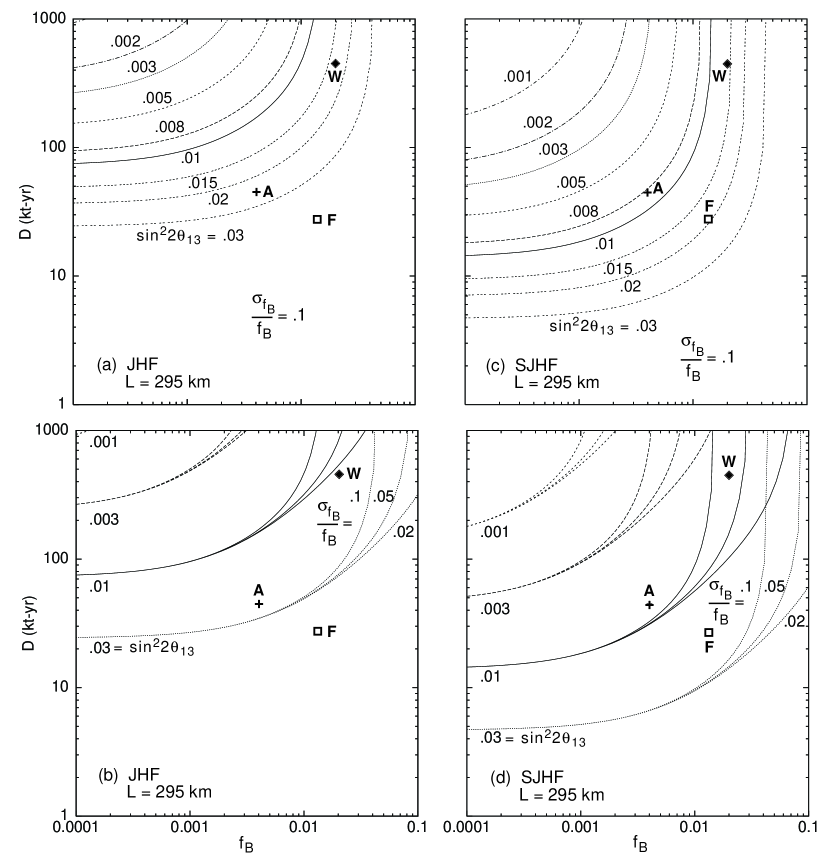
We can now investigate the dependence of the reach on the detector parameters, and hence try to understand whether a massive water Cherenkov detector is likely to be the best option. In Fig. 1 contours of constant reach are shown as a function of the dataset size and the background rate for 3 years of running at the 0.77 MW JHF beam (left-hand plots) and at an upgraded 4 MW SJHF beam (right-hand plots). The lower panels show how the reach varies with . The contours have a characteristic shape. At sufficiently large the sensitivity is limited by the systematic uncertainties associated with the background subtraction, and the reach does not significantly improve with increasing dataset size. The contours are therefore vertical in this region of Fig. 1. At sufficiently small the sensitivity of the appearance search is limited by signal statistics, and further reductions in do not improve the reach. The contours are therefore horizontal in this region of Fig. 1. The positions in the (, )-plane corresponding to our three detector scenarios (, , and ) are indicated on the figure. For the 0.77 MW machine the two scenarios ( and ) both yield reaches in the range 0.015 to 0.03. However, the water Cherenkov sensitivity is limited by the systematic uncertainty on the substantial background. Hence, the reach for scenario does not improve substantially when the accelerator beam is upgraded from 0.77 MW to 4 MW (SJHF). On the other hand this upgrade would result in a substantial improvement in the reach obtained with scenario , which is not background limited, and therefore has a reach improving almost linearly with . We conclude that, even with SJHF, it will be difficult to observe a signal if is less than about 0.01. This conclusion is consistent with the JHF study group analysis, but is in conflict with the expectations of Ref. [33]. On the positive side, if is larger than 0.01, a 1 GeV neutrino beam at JHF or SJHF would permit the observation of a signal. Detector scenario does slightly better for a 0.77 MW JHF, while scenario does slightly better for a 4.0 MW SJHF.
Finally, we consider whether the reach at a 1 GeV JHF or SJHF neutrino beam can be improved with a different choice of baseline. Contours of constant reach in the ()-plane are shown for scenarios and in Fig. 2. A baseline of 295 km does indeed yield the optimal reach for the water Cherenkov scenario. For scenario , a slightly shorter baseline (200 km) would yield a slightly improved reach.
B Sensitivities for long baseline experiments
1 Decay channel length restrictions
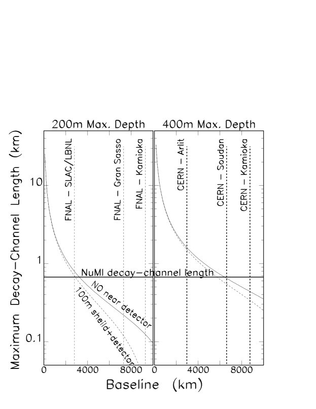
Consider next the sensitivity that can be achieved with longer baselines and higher energies. We begin by considering how restrictions on the decay channel length reduce the neutrino flux for very long baselines. In a conventional neutrino beamline design it is desirable that the pion decay channel is long enough for most of the pions to decay. However, for very-long-baseline experiments the decay channel must point downwards at a steep angle, and the geology under the accelerator site may impose significant constraints on the maximum length of the decay channel. In practice, an upgraded long-baseline conventional neutrino beam would be sited at an existing particle physics laboratory having a high-energy proton accelerator: Brookhaven or Fermilab in the US, CERN or DESY in Europe, or the planned JHF laboratory in Japan. The rock characteristics under the JHF site are expected to be determined next year by drilling [70]. The site with the deepest viable rock layer in the US is Fermilab, which sits above approximately 200 m of good rock. The Brookhaven and DESY [74] laboratories sit just above the water table — an impediment that would have to be overcome before a high-energy long-baseline beam could be proposed. The depth of the good rock (Molasse) under CERN varies between about 200 m and 400 m, depending on location [72]. The impact of these restrictions on the maximum decay channel length is shown as a function of the baseline length in Fig. 3 for the Fermilab and CERN sites. The resulting fraction of pions that decay within the decay channel is summarized in Table II for several neutrino beam energies. The channel length calculations were performed assuming that (i) the proton accelerator is at a depth of 10 m, (ii) the beam is then bent down to point in the appropriate baseline-dependent direction using a magnetic channel with an average field of 2 Tesla, and (iii) once pointing in the right direction the proton beam enters a 50 m long targeting and focusing section, after which the decay channel begins. The maximum decay channel length then depends upon whether the channel extends all the way to the bottom of the usable rock layer, or whether this rock layer must also accommodate a near detector. Results for both of these cases are presented in Fig. 3 and Table II. In the near-detector case the maximum decay channel length has been reduced by 100 m to allow for the shielding and detector hall. The pion decay fraction estimates have been made assuming that all of the decaying pions have the average pion energy in the channel.
The decay fractions in Table II show that the site-dependent depth restrictions will result in a significant reduction in the neutrino beam intensities for high-energy long-baseline beams. For example, at the Fermilab site there is no room for a near detector if the baseline is 9300 km (Fermilab to SuperK). With the medium energy beam and a baseline of 7300 km (Fermilab to Gran Sasso) only 17% of the pions decay within the channel. Hence, the channel length restrictions would exclude, or at least heavily penalize, the extremely-long-baseline ideas proposed by Dick et al. [75]. Clearly, decay channel length restrictions must be taken into account when comparing choices of baseline and beam energy.
2 reach for scenarios and
We are now ready to consider the reach that can be obtained in a long-baseline experiment. In our main discussion we consider appearance with ; the case is discussed at the end of this section. Our calculations use the WBB spectra and interaction rates presented in the MINOS design report [14] for the low-energy (LE) horn configuration ( GeV), the medium-energy (ME) horn configuration ( GeV), and the high-energy (HE) horn configuration ( GeV). After accounting for the decay channel length restrictions arising from a maximum depth requirement of 200 m, the neutrino fluxes are assumed to scale with the inverse square of the baseline length.
The calculated reaches are listed in Tables III and IV for detector scenarios and , and several baselines: km (Fermilab Soudan or CERN Gran Sasso), km (Fermilab LBNL/SLAC), km (Fermilab Gran Sasso), and km (Fermilab SuperK). Note that the shortest baseline (730 km) has a very limited reach for all the beams, and the lowest energy beam (LE) has a very limited reach for all baselines. The best reach for detector scenario is , which is obtained with a baseline that is not too long (e.g. 2900 km). The best reach for detector scenario is also , and is obtained with long baselines (e.g. 7300 km or 9300 km) which benefit from the enhancement of the oscillation amplitude due to matter effects. The reaches for the two longest baselines are about the same since the increase of the matter enhancement as increases is compensated by the decrease in the pion decay fraction due to the decay channel length restriction.
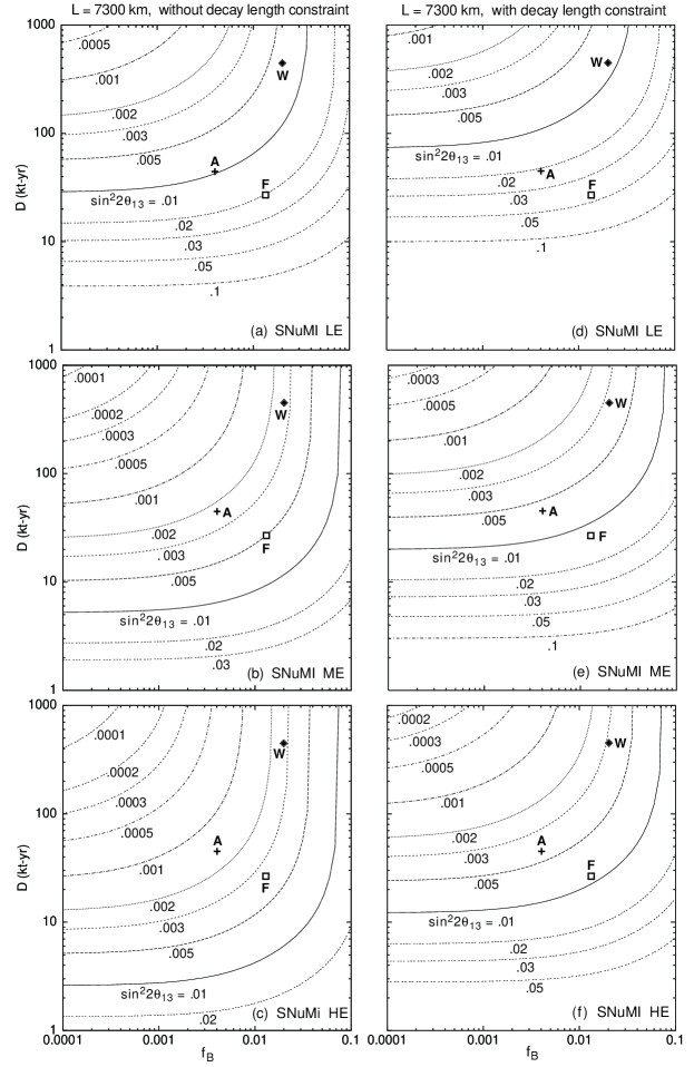
To further illustrate the impact of the decay channel length restrictions on the reach for long-baseline experiments, in Fig. 4 contours of constant reach are shown in the (, )-plane for km with the channel length restrictions (right-hand plots) and without the channel length restrictions (left-hand plots). The scenario point lies in the systematics-dominated (vertical contour) region, and is therefore not significantly affected by a reduction in due to the decay channel length restrictions. However, the scenario point lies between the systematics-limited and statistics-limited regions of the plot, and is significantly affected by the reduction in neutrino flux due to the channel length restrictions. Indeed, in scenario the reach at the HE beam is degraded from about 0.0015 to about 0.004 by the channel length restriction.
3 Dependence on detector parameters
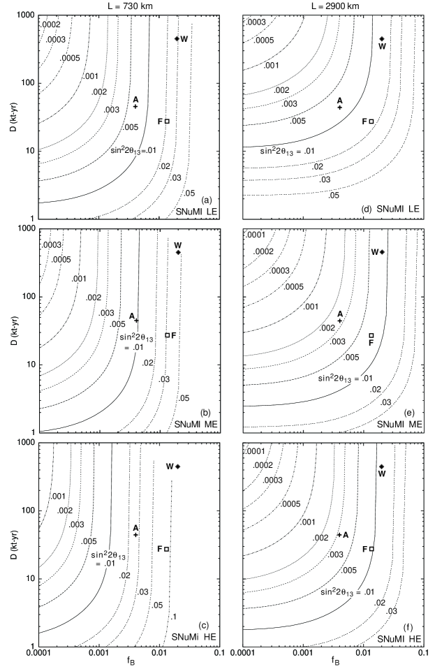
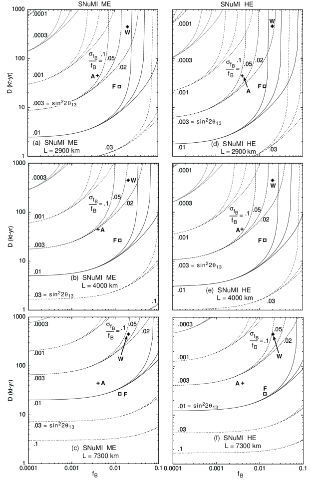
We can now explore the dependence of the reach on the baseline, beam energy, and detector parameters. In Fig. 5 contours of constant reach are shown in the (, )-plane for km and 2900 km. As already noted, for our detector scenarios and the best reach is , obtained with scenario at km using either the ME or HE beams (Figs. 5e and 5f), or with scenario at km using the same beams (Figs. 4e and 4f). It is interesting to consider what improvements to scenarios and would be required to obtain a reach of 0.001, for example. This goal can be attained by decreasing the background fraction for scenario to (or alternatively increasing the dataset size for scenario by a factor of 10) and using the HE beam at a very long baseline. The goal could also be attained by decreasing for scenario by an order of magnitude and using the high energy beam and a baseline of 2900 km, for example. None of these revised detector scenarios seems practical. An alternative strategy is to try to find a detector scenario with a smaller systematic uncertainty on . Fig. 6 shows, for the ME and HE beams, contours of constant reach in the (, )-plane for several different , and for baselines of 2900 km, 4000 km, and 7300 km. The scenario sensitivity would benefit if the systematic uncertainty on the background could be reduced, but even a factor of five improvement in would not permit a reach of 0.001 to be attained.
Since detector scenarios and are ambitious, we can ask what happens if , , or must be relaxed. The best reaches obtained with scenario were for the ME and HE beams at very long baselines (e.g. km). In these cases the reach is not very sensitive to , but degrades roughly linearly with increasing (Fig. 4) or (Fig. 6). Hence, if the achievable background rate is really then the reach is well above 0.01 for the observation of a signal at 3 standard deviations above the background. The best reaches obtained with scenario were for the ME and HE beams at long baselines (e.g. km). In these cases the reach is sensitive to both decreases in and increases in . The reach can be degraded by a factor of 2 by either reducing by about a factor of 4, or by increasing by about a factor of 3 (Fig. 5).
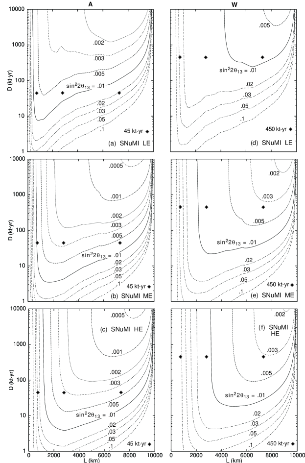
So far we have considered only a few discrete baseline lengths. To explore the reach that can be obtained with other baseline choices, Fig. 7 shows, for each of the three NuMI beam energies, contours of constant reach in the (, )-plane for scenarios and . For scenario , where backgrounds are less important, the optimal distance varies with beam energy; crudely speaking, the optimal is given by making the vacuum oscillation argument of order . For scenario the backgrounds are more important and larger distances give a better reach for all three upgraded NuMI beams.
Finally, we have also studied neutrino beams with higher energy than NuMI. For example, the CNGS beam [76] at CERN has an average neutrino energy of about 20 GeV. We find that for the expected protons on target per year, three years of running will at best give a reach of about 0.01 for either scenario or . Upgrading the proton intensity by a factor of four improves the reach to about 0.005. Therefore we conclude that the higher-energy CNGS superbeams have similar capability to the SNuMI beams.
4 Summary of reaches for and
In summary, Figs. 4, 5, and 7 show that the best reach that can be obtained with detector scenarios and is about 0.003. This optimum reach can be obtained in scenario with – km for the NuMI ME beam or with – km for the HE beam, or in scenario with – km for either the ME or HE beams. Scenarios and require ambitious detector parameters. To improve the reach to 0.001, for example, requires substantial improvements in , , and/or , and does not therefore seem practical. If the scenario and parameters cannot be realized the reach will be degraded. In particular, a significant increase of (or ) in either scenario or would result in a significant decrease in reach. A significant decrease in the data-sample size in scenario will also degrade the reach.
Up to now we have considered the sensitivity of long baseline experiments if . We now turn our attention to the alternative case: . In this case long baseline experiments using a neutrino beam will suffer from a suppression of signal due to matter effects. Therefore, in our scenarios and , if no signal is observed after 3 years of neutrino running the beam is switched to antineutrinos for a further 6 years of data taking. For antineutrino running with the results shown in Figs. 4, 5, and 7 must be modified since the antineutrino cross section is about half of the neutrino cross section. Hence we must double the required values on the -axes in the various figures. Other modifications to the contour plots for antineutrino running with are minor since the matter enhancement in this case is similar to the enhancement for neutrinos when (they are the same in the limit that the sub-leading oscillation can be ignored). However, the positions of the scenario and points on the various figures must be moved to account for the larger values of and (and potentially ). Note that the larger background rate associated with antineutrino running in Scenario will degrade the ultimate reach for ; the best reach becomes .
V Neutrino mass hierarchy and CP-violation
In the 1 GeV and multi-GeV superbeam scenarios that we have considered it will be difficult to observe a or signal if is smaller than about 0.01. However, if is (0.01) a signal would be observable provided a sufficiently massive detector with sufficiently small background is practical. We would like to know if, in this case, the sign of can be determined in the long-baseline multi-GeV beam experiment, and whether violation might be observed in either the long-baseline multi-GeV beam experiment or the 1 GeV intermediate baseline experiment. We begin by considering the sensitivity at the SJHF, and then consider the sensitivity for determining violation and/or the pattern of neutrino masses at long baselines.
A violation with a JHF superbeam
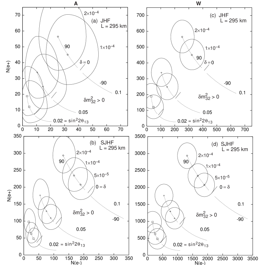
In our SJHF scenario, a violation search would consist of running for 3 years with a neutrino beam and measuring the number of signal events [], and then running for 6 years with an antineutrino beam and measuring the number of signal events []. In our calculations we assume that the antineutrino cross section is about one-half of the neutrino cross section, and that the antineutrino flux is the same as the neutrino flux. In the absence of violation ( or ), after correcting for cross-section and flux differences, we would therefore expect . In the presence of maximal violation with we would expect . The magnitude of the deviation from induced by violation is quite sensitive to the sub-leading scale . Setting , in Fig. 8 the predicted positions in the []-plane are shown for scenarios (left-hand plots) and (right-hand plots) The predictions are shown as a function of both and . The error ellipses around each point indicate the measurement precision at 3 standard deviations, taking into account both statistical and systematic uncertainties, and using the statistical prescription described in the appendix. An overall normalization uncertainty (which could account for uncertainties in the flux and/or cross sections) of 2% is included, although its effects are generally small. violation can be established at the level if the error ellipses do not overlap the -conserving curves (solid lines, ). The curves for the other -conserving case () lie very close to the curves and are not shown.
Note that for scenario with the upgraded 4 MW SJHF beam, if (larger values are already excluded), eV2, and , then the predicted point in the []-plane is just away from the conserving () prediction. Alternatively, if , eV2 (larger values are improbable), and , then the predicted point is also just away from the -conserving prediction. Hence there is a small region of the allowed parameter space ( and eV2) within which maximal violation might be observable at an upgraded JHF if is in the center of the presently favored SuperK region and . It is also possible to detect maximal violation for and eV2 with the 0.77 MW JHF in the scenario. Generally detector scenario does better for violation, except scenario is slightly better for at the 4 MW SJHF. Because the matter effect is small at km, predictions for and are nearly the same, and hence the sign of cannot be determined.
B violation and the sign of at long-baseline experiments
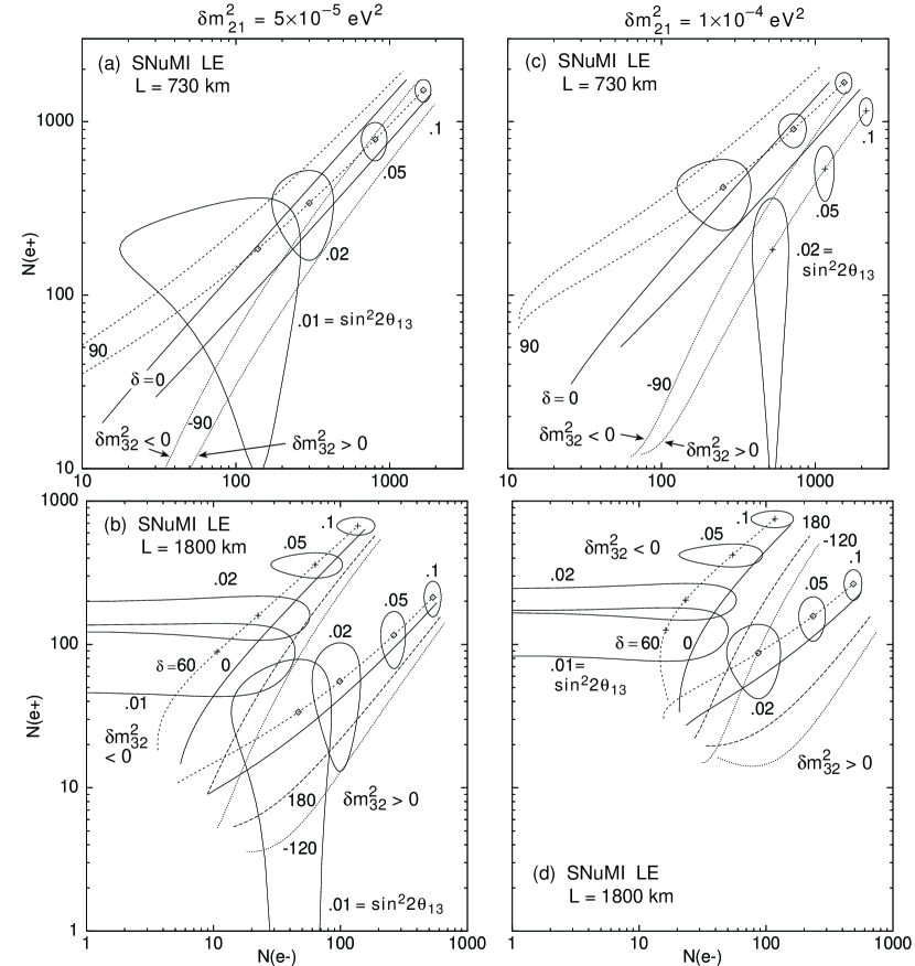
Consider next long-baseline experiments using multi-GeV neutrino beams. The approximate equality will be modified by intrinsic violation and by matter effects. Predictions in the []-plane are shown in Fig. 9 for scenario using the 1.6 MW LE superbeam for two values of ( eV2 and eV2), and for two baselines ( km and 1800 km). The predictions for each of these cases are shown as a function of , , and the sign of , with eV2 and . Note that at km the magnitude of the modifications of the appearance rates due to matter effects are comparable to the magnitudes of the modifications due to maximal intrinsic violation. Furthermore, the expected precisions of the measurements, shown on the figure by the error ellipses, are also comparable to the sizes of the predicted and matter effects.
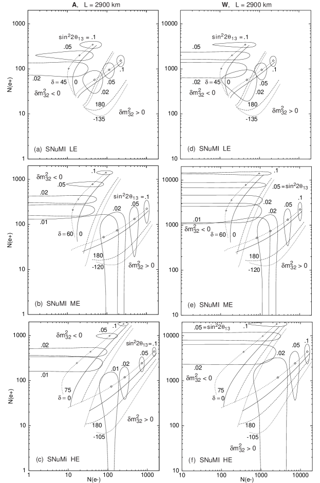
Matter effects will cause the two -conserving cases and to give different predictions for and , and therefore to establish violation the signal must be distinguishable from both and . Hence, in the scenario we are considering, Fig. 9 shows that superbeam measurements with the LE beam at 730 km can help to constrain the parameter space, but generally cannot provide unambiguous evidence for intrinsic violation, and cannot unambiguously determine the sign of . The only exception to this is if and (or and ), in which case violation could be established and the sign of determined for . The and matter effects are better separated at km, for which an unambiguous determination of the sign of seems possible provided , although violation cannot be established for eV2. At smaller values of modifications to the appearance rates cannot distinguish between matter and effects. Note that, because of the matter effect, at distances longer than 1000 km the values of that give the largest disparity of and are no longer . Also note that the sign of is most easily determined when the and matter effects interfere constructively to give a greater disparity of and , and more difficult when the and matter effects interfere destructively [i.e., and are more equal]. Going to even longer baselines, predictions in the [] plane are shown in Fig. 10 for scenario (left-hand plots) and scenario (right-hand plots) with km. The predictions are shown for the LE beam (top plots), ME beam (middle plots), and HE beam (bottom plots). In general, the sign of can be determined provided , but in none of the explored long-baseline scenarios can -violation be unambiguously established for eV2.
C CP-violation and the sign of at a neutrino factory
We can ask, how do the and -sign capabilities of superbeams compare with those of a neutrino factory? The relevant experimental signature at neutrino factory is the appearance of a wrong-sign muon indicating (or ) transitions. This is a much cleaner signature than electron appearance with a superbeam. Hence, background systematics are under better control at a neutrino factory, and the expected error ellipses in the [N(), N()]-plane are therefore much smaller.
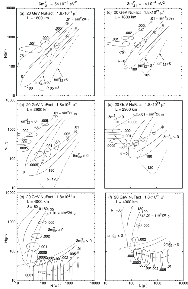
In our analysis we assume a 20 GeV neutrino factory with useful decays (which might be achieved in three years running at at high-performance neutrino factory) and useful decays, a 50 kt iron–scintillator detector [49] at distances km, 2900 km, and 4000 km from the source. For comparison, the total neutrino flux for three years running at a distance of 1 km from the source is for the neutrino factory scenario, while it is for SJHF and for the SNuMI HE beam. We choose an iron–scintillator detector for the neutrino factory analysis since it is particularly well–suited for the detection of muons and can be made larger than, e.g., a liquid argon detector, at a similar or lower cost. We also take , , and a normalization uncertainty of 2%. This background level can be achieved with a 4 GeV cut on the detected muon, which gives a detection efficiency of about 73%, implying an effective data sample of kt–yr for three years running.
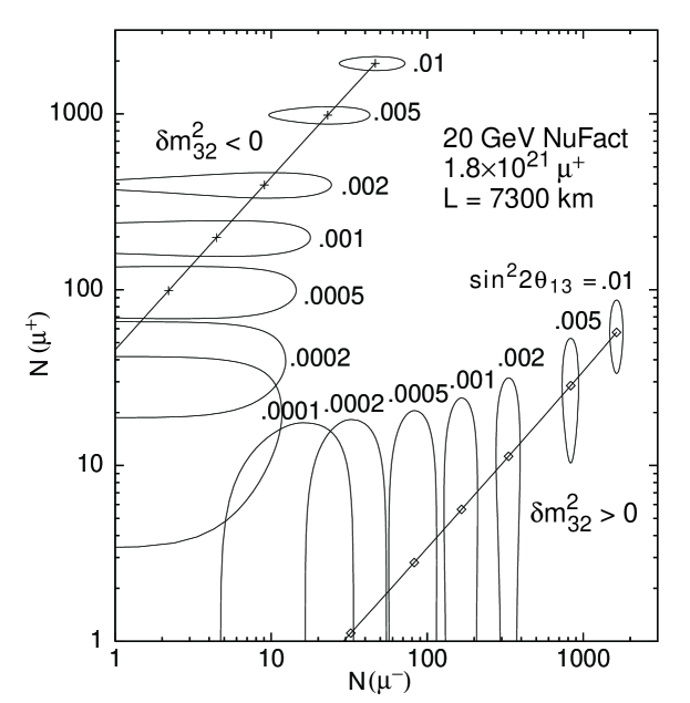
The corresponding neutrino factory predictions in the [N(), N()]-plane are shown in Fig. 11. The 1800 km baseline is too short, since matter and effects are indistinguishable in most cases. At 2900 km the predictions allow an unambiguous determination of the sign of for much of the parameter space, and the possibility of establishing the existence of . At 4000 km the statistical uncertainties are larger, and impair the sensitivity to observe . However, matter effects are also larger, and an unambiguous determination of the sign of is possible down to of a few . For very long baselines (e.g. km, Fig. 12) there is negligible sensitivity to or to , matter effects are large, and the reach for determining the sign of approaches .
VI Summary
We have explored the oscillation-physics capabilities of 1 GeV and multi-GeV neutrino beams produced at MW-scale proton accelerator facilities (neutrino superbeams). Specifically, the limiting value of that would permit the first observation of and/or oscillations at 3 standard deviations is considered, along with the ability of these intense conventional neutrino beams to determine the pattern of neutrino masses (sign of ) and discover -violation in the lepton sector. The figures in this paper provide a toolkit for accessing the physics capabilities as a function of the detector specifications, characterized by the dataset size (kt-years) and the uncertainty on the background subtraction (given by and ). Table V summarizes the physics capabilities of some beam-detector combinations. Also shown in the table are similar results for an entry-level and high-performance neutrino factory with GeV.
Determining the optimum detector technology and characteristics is beyond the scope of this paper, and may require a detector R&D program. However, for some ambitious but plausible detector scenarios we find:
-
(i) With a sufficiently ambitious detector, if few and , then and signals should be observable at a superbeam. The reach is slightly worse if . The best reach is obtained with a long-baseline multi-GeV superbeam; for example, with the SNuMI ME or HE beams and a baseline km. This would permit the tightening of constraints on the oscillation parameter space. It is important to account for decay channel length restrictions when assessing the capabilities of very-long-baseline experiments.
-
(ii) If is maximally violated in the lepton sector, there is a small region of allowed parameter space in which an experiment at a JHF or SJHF beam ( GeV) might be able to establish -violation at 3 standard deviations. Except for certain small regions in parameter space where matter and effects constructively interfere, a long-baseline experiment with conventional superbeams would be unable to unambiguously establish violation because matter effects can confuse the interpretation of the measurements.
-
(iii) With a sufficiently ambitious detector, if there is a significant region of parameter space over which a long baseline experiment with a multi-GeV neutrino superbeam could unambiguously establish the sign of .
-
(iv) Lower-energy superbeams do best at shorter distances, with a fair reach for appearance and some capability, but little or no sensitivity to the sign of ; higher-energy superbeams do best at longer distances, with good reach for appearance and sign() determination, but little or no sensitivity to .
-
(v) A neutrino factory can deliver between one and two orders of magnitude better reach in for appearance, the sign of , and violation; for km there is excellent sensitivity to all three observables.
Acknowledgments
This research was supported in part by the U.S. Department of Energy under Grants No. DE-FG02-94ER40817, No. DE-FG02-95ER40896 and No. DE-AC02-76CH03000, and in part by the University of Wisconsin Research Committee with funds granted by the Wisconsin Alumni Research Foundation.
REFERENCES
- [1] Super-Kamiokande Collaboration, Y. Fukuda et al., Phys. Lett. B433, 9 (1998); Phys. Lett. B436, 33 (1998); Phys. Rev. Lett. 81, 1562 (1998); Phys. Rev. Lett. 82, 2644 (1999).
- [2] Kamiokande collaboration, K.S. Hirata et al., Phys. Lett. B280, 146 (1992); Y. Fukuda et al., Phys. Lett. B335, 237 (1994); IMB collaboration, R. Becker-Szendy et al., Nucl. Phys. Proc. Suppl. 38B, 331 (1995); Soudan-2 collaboration, W.W.M. Allison et al., Phys. Lett. B391, 491 (1997); MACRO collaboration, M. Ambrosio et al., Phys. Lett. B434, 451 (1998).
- [3] G. Barr, T.K. Gaisser, and T. Stanev, Phys. Rev. D39, 3532 (1989); M. Honda, T. Kajita, K. Kasahara, and S. Midorikawa, Phys. Rev. D52, 4985 (1995); V. Agrawal, T.K. Gaisser, P. Lipari, and T. Stanev, Phys. Rev. D53, 1314 (1996); T.K. Gaisser et al., Phys. Rev. D54, 5578 (1996); T.K. Gaisser and T. Stanev, Phys. Rev. D57, 1977 (1998); P. Lipari, Astropart. Phys. 14, 153 (2000).
- [4] V. Barger and K. Whisnant, Phys. Lett. 209B, 365 (1988); J.G. Learned, S. Pakvasa, and T.J. Weiler, ibid. 207B, 79 (1988); K. Hidaka, M. Honda, and S. Midorikawa, Phys. Rev. Lett. 61, 1537 (1988).
- [5] S.M. Bilenky, C. Giunti, and W. Grimus, Eur. Phys. J. C1, 247 (1998); V. Barger, K. Whisnant, and T.J. Weiler, Phys. Lett. B427, 97 (1998); V. Barger, S. Pakvasa, T.J. Weiler, and K. Whisnant, Phys. Rev. D58, 093016 (1998); V. Barger, Yuan-Ben Dai, K. Whisnant, and B.-L. Young, Phys. Rev. D59, 113010 (1999); O. Yasuda, talk given at 30th International Conference on High-Energy Physics (ICHEP 2000), Osaka, Japan, Aug. 2000, hep-ph/0008256; T. Hattori, T. Hasuike, and S. Wakaizumi, hep-ph/0010232. Additional references can be found in V. Barger and K. Whisnant, hep-ph/0006235, to be published in “Current Aspects of Neutrino Physics”, ed. by D. Caldwell (Springer-Verlag, Hamburg, 2000).
- [6] CHOOZ Collaboration, M. Apollonio et al., Phys. Lett. B420, 320 (1998); Palo Verde Collaboration, C. Gratta, talk at Neutrino-2000, XIXth International Conference on Neutrino Physics and Astrophysics, Sudbury, Canada, June 2000.
- [7] L. Wolfenstein, Phys. Rev. D17, 2369 (1978); V. Barger, S. Pakvasa, R.J.N. Phillips, and K. Whisnant, Phys. Rev. D22, 2718 (1980).
- [8] V. Barger, N. Deshpande, P. B. Pal, R.J.N. Phillips, and K. Whisnant, Phys. Rev. D43 (Rapid Communications), R1759 (1991).
- [9] T. Toshita, talk given at 30th International Conference on High-Energy Physics (ICHEP 2000), Osaka, Japan, Aug. 2000.
- [10] G.L. Fogli, E. Lisi, A. Marrone, hep-ph/0009299.
- [11] V. Barger, J.G. Learned, S. Pakvasa, and T.J. Weiler, Phys. Rev. Lett. 82, 2640 (1999); V. Barger, J.G. Learned, P. Lipari, M. Lusignoli, S. Pakvasa, and T.J. Weiler, Phys. Lett. B462, 109 (1999).
- [12] A. Acker, A. Joshipura, and S. Pakvasa, Phys. Lett. B285, 371 (1992); G. Gelmini and J.W.F. Valle, Phys. Lett. B142, 181 (1984); K. Choi and A. Santamaria, Phys. Lett. B267, 504 (1991); A.S. Joshipura, PRL Report-PRL-TH-91/6; A.S. Joshipura and S. Rindani, Phys. Rev. D46, 3000 (1992).
- [13] K. Nishikawa et al. (KEK-PS E362 Collab.), “Proposal for a Long Baseline Neutrino Oscillation Experiment, using KEK-PS and Super-Kamiokande”, 1995, unpublished; talk presented by M. Sakuda (K2K collaboration) at the XXXth International Conference on High Energy Physics (ICHEP 2000), Osaka, Japan, July 2000.
- [14] MINOS Collaboration, “Neutrino Oscillation Physics at Fermilab: The NuMI-MINOS Project,” NuMI-L-375, May 1998.
- [15] See the ICARUS/ICANOE web page at http://pcnometh4.cern.ch/
- [16] See the OPERA web page at http://www.cern.ch/opera/
- [17] B.T. Cleveland et al., Nucl. Phys. B (Proc. Suppl.) 38, 47 (1995).
- [18] Kamiokande collaboration, Y. Fukuda et al., Phys. Rev. Lett, 77, 1683 (1996).
- [19] Super-Kamiokande collaboration, Y. Fukuda et al., Phys. Rev. Lett. 81, 1158 (1998); 82, 1810 (1999); 82, 2430 (1999).
- [20] GALLEX collaboration, W. Hampel et al., Phys. Lett. B388, 384 (1996); SAGE collaboration, J.N. Abdurashitov et al., Phys. Rev. Lett. 77, 4708 (1996); GNO Collaboration, M. Altmann et al., hep-ex/0006034.
- [21] J.N. Bahcall and M.H. Pinsonneault, Rev. Mod. Phys. 67, 781 (1995); J.N. Bahcall, S. Basu, and M.H. Pinsonneault, Phys. Lett. B 433, 1 (1998).
- [22] N. Hata and P. Langacker, Phys. Rev. D56, 6107 (1997); J.N. Bahcall, M.H. Pinsonneault, and S. Basu, astro-ph/0010346.
- [23] Y. Takeuchi, talk given at 30th International Conference on High-Energy Physics (ICHEP 2000), Osaka, Japan, Aug. 2000.
- [24] S.P. Mikheyev and A. Smirnov, Yad. Fiz. 42, 1441 (1985) [Sov. J. Nucl. Phys. 42, 913 (1986)]; P. Langacker, J.P. Leveille, and J. Sheiman, Phys. Rev. D 27, 1228 (1983).
- [25] G. Fogli, E. Lisi, D. Montanino, and A. Palazzo, hep-ph/0008012; M.C. Gonzalez-Garcia, C. Pena-Garay, Y. Nir, A. Yu. Smirnov, hep-ph/0007227; J.N. Bahcall, P.I. Krastev, A. Yu. Smirnov, Phys. Rev. D60, 093001 (1999); J.N. Bahcall and P.I. Krastev, Phys. Rev. C56, 2839 (1997); M. Maris and S. Petcov, Phys. Rev. 58, 113008 (1998); Phys. Rev. D56, 7444 (1997); hep-ph/0004151; Q.Y. Liu, M. Maris and S. Petcov, Phys. Rev. 56, 5991 (1997); E. Lisi and D. Montanino, Phys. Rev. D56, 1792 (1997). A.H. Guth, L. Randall, and M. Serna, JHEP 9908, 019 (1999). A. de Gouvea, A. Friedland, and H. Murayama, hep-ph/9910286.
- [26] M.C. Gonzales-Garcia and C. Pena-Garay, hep-ph/009041; M.C. Gonzalez-Garcia, M. Maltoni, C. Pena-Garay, J.W.F. Valle, hep-ph/0009350; R. Barbieri and A. Strumia, hep-ph/0011307.
- [27] V. Barger, B. Kayser, J.G. Learned, T.J. Weiler, and K. Whisnant, hep-ph/0008019, Phys. Lett. B489, 345 (2000).
- [28] O.L.G. Peres and A. Yu. Smirnov, hep-ph/0011054.
- [29] KamLAND proposal, Stanford-HEP-98-03; A. Piepke, talk at Neutrino-2000, XIXth International Conference on Neutrino Physics and Astrophysics, Sudbury, Canada, June 2000.
- [30] V. Barger, D. Marfatia, and B.W. Wood, hep-ph/0011251.
- [31] C. Athanassopoulos et al. (LSND Collab.), Phys. Rev. Lett. 77, 3082 (1996); 81, 1774 (1998); G. Mills, talk at Neutrino-2000, XIXth International Conference on Neutrino Physics and Astrophysics, Sudbury, Canada, June 2000.
- [32] A. Bazarko, MiniBooNE Collaboration, talk at Neutrino-2000.
- [33] B. Richter, hep-ph/0008222
- [34] K. Dick, M. Freund, P. Huber, and M. Lindner, hep-ph/0008016.
- [35] S. Geer, Phys. Rev. D57, 6989 (1998).
- [36] V. Barger, S. Geer, and K. Whisnant, Phys. Rev. D61, 053004 (2000).
- [37] V. Barger, S. Geer, R. Raja, and K. Whisnant, hep-ph/0007181, to appear in Phys. Rev. D.
- [38] V. Barger, S. Geer, R. Raja, and K. Whisnant, Phys. Lett. B485, 379 (2000).
- [39] H.W. Zaglauer and K.H. Schwarzer, Z. Phys. C40, 273 (1988).
- [40] R.H. Bernstein and S.J. Parke, Phys. Rev. D44, 2069 (1991).
- [41] V. Barger, S. Geer, R. Raja, and K. Whisnant, Phys. Rev. D62, 013004 (2000).
- [42] V. Barger, S. Geer, R. Raja, and K. Whisnant, Phys. Rev. D62, 073002 (2000).
- [43] P. Lipari, Phys. Rev. D61, 113004 (2000).
- [44] A. De Rujula, M.B. Gavela, and P. Hernandez, Nucl. Phys. B547, 21 (1999).
- [45] A. Donini, M.B. Gavela, P. Hernandez, and S. Rigolin, Nucl. Phys. B574, 23 (2000); A. Cervera, A. Donini, M.B. Gavela, J.J. Gomez Cadenas, P. Hernandez, O. Mena, and S. Rigolin, hep-ph/0002108.
- [46] K. Dick, M. Freund, M. Lindner, and A. Romanino, Nucl. Phys. B562, 299 (1999); A. Romanino, Nucl. Phys. B574, 675 (2000); M. Freund, M. Lindner, S.T. Petcov, and A. Romanino, Nucl. Phys. B578, 27 (2000).
- [47] M. Freund, P. Huber, and M. Lindner, Nucl. Phys. B585, 105 (2000).
- [48] D. Ayres et al., Neutrino Factory and Muon Collider Collaboration, physics/9911009.
- [49] C. Albright et al., hep-ex/0008064.
- [50] M. Campanelli, A. Bueno, and A. Rubbia, hep-ph/9905240; A. Bueno, M. Campanelli, and A. Rubbia, Nucl. Phys. B573, 27 (2000); Nucl. Phys. B589, 577 (2000).
- [51] M. Koike and J. Sato, Phys. Rev. D61, 073012 (2000).
- [52] O. Yasuda, hep-ph/0005134.
- [53] P.F. Harrison and W.G. Scott, Phys. Lett. B476, 349 (2000); H. Yokomakura, K. Kimura, and A. Takamura, hep-ph/0009141; S.J. Parke and T.J. Weiler, hep-ph/0011247; Z.Z. Xing, Phys. Lett. B487, 327 (2000) and hep-ph/0009294.
- [54] J. Arafune and J. Sato, Phys. Rev. D55, 1653 (1997); M. Koike and J. Sato, hep-ph/9707203; J. Arafune, M. Koike, and J. Sato, Phys. Rev. D56, 3093 (1997); T. Ota and J. Sato, hep-ph/0011234.
- [55] T. Hattori, T. Hasuike, and S. Wakaizumi, Phys. Rev. D62, 033006 (2000).
- [56] V. Barger, R.J.N. Phillips, and K. Whisnant, Phys. Rev. Lett. 45, 2084 (1980).
- [57] S. Pakvasa, in High Energy Physics – 1980, AIP Conf. Proc. No. 68, ed. by L. Durand and L.G. Pondrom (AIP, New York, 1981), p. 1164.
- [58] T.K. Kuo and J. Pantaleone, Rev. Mod. Phys. 61, 937 (1989).
- [59] Parameters of the Preliminary Reference Earth Model are given by A. Dziewonski, Earth Structure, Global, in “The Encyclopedia of Solid Earth Geophysics”, ed. by D.E. James, (Van Nostrand Reinhold, New York, 1989) p. 331; also see R. Gandhi, C. Quigg, M. Hall Reno, and I. Sarcevic, Astroparticle Physics 5, 81 (1996).
- [60] W.-Y. Keung and L.-L. Chau, Phys. Rev. Lett. 53, 1802 (1984).
- [61] C. Jarlskog, Z. Phys. C 29, 491 (1985); Phys. Rev. D35, 1685 (1987).
- [62] S. Coleman and S.L. Glashow, Phys. Rev. D59, 116008 (1999).
- [63] V. Barger, S. Pakvasa, T.J. Weiler, and K. Whisnant, hep-ph/0005197, Phys. Rev. Lett. (in press).
- [64] H. Murayama and T. Yanagida, hep-ph/0010178.
-
[65]
Talk presented by W. Marciano at the Joint U.S./Japan Workshop On New
Initiatives In Muon Lepton Flavor Violation and Neutrino Oscillation
With High Intense Muon and Neutrino Sources, Honolulu, Hawaii,
Oct. 2–6, 2000,
http://meco.ps.uci.edu/lepton_workshop/talks/marciano.pdf. - [66] I. Mocioiu and R. Shrock, AIP Conf. Proc. 533, 74 (2000); Phys. Rev. D62, 053017 (2000).
- [67] J. Pantaleone, Phys. Rev. Lett. 81, 5060 (1998).
- [68] JHF LOI, http://www-jhf.kek.jp/
- [69] See also talks by D. Casper, K. Nakamura, Y. Obayashi, and Y.F. Wang at the Joint U.S./Japan Workshop On New Initiatives In Muon Lepton Flavor Violation and Neutrino Oscillation With High Intense Muon and Neutrino Sources, Honolulu, Hawaii, Oct. 2–6, 2000, http://meco.ps.uci.edu/lepton_workshop/talks/
- [70] M. Aoki, private communication
- [71] W. Chou, FERMILAB-Conf-97/199, Proc. 1997 Particle Accel. Conf. PAC97, Vancouver, Canada, May 1997.
- [72] M. Campanelli, private communication.
- [73] L. Barret et al., NuMI-L-551 (1999).
- [74] N. Holtkamp, private communication.
- [75] K. Dick, M. Freund, P. Huber, and M. Lindner, Nucl. Phys. B588, 101 (2000).
- [76] CNGS conceptual design report, CERN 98-02.
-
[77]
Talk presented by A. Riche at the Joint U.S. / Japan Workshop On
New Initiatives In Muon Lepton Flavor Violation And Neutrino Oscillation
With High Intense Muon And Neutrino Sources, Honolulu, Hawaii, Oct. 2000,
http://meco.ps.uci.edu/lepton_workshop/talks/riche.pdf - [78] V. Barger, S. Geer, R. Raja, and K. Whisnant, in preparation.
- [79] N. Gehrels, Ap. J 303, 336 (1986).
Appendix
To implement the Poisson statistical uncertainties in our analysis of the reach we use an approximate expression for the upper limit () on the number of events from the observation of events,
| (35) |
where is the number of standard deviations corresponding to the limit. This expression gives the correct with an accuracy that is better than 10% for , and better than 1% for larger [79]. If the number of predicted background events is , the expected number of signal events corresponding to an observation 3 statistical standard deviations above the background is given by
| (36) |
Let the systematic uncertainty on be given by . To account for this systematic uncertainty, we add it in quadrature with the statistical uncertainty. Defining the quantity
| (37) |
the reach can then be estimated by finding the value of that yields signal events.
To determine the sign of and/or search for violation with conventional and beams, we will need to compare the and appearance rates (for a neutrino factory with a detector that measures muons, we compare the and appearance rates). As in the case of the reach, we will be considering the allowed regions.
Let and be the number of events that satisfy the signal selection criteria and are recorded respectively during neutrino and antineutrino running. If and are theoretical predictions for and , the region of the – space allowed by the measurements is described by
| (38) |
where and are the experimental uncertainties on and , respectively. In the absence of systematic uncertainties, and in the approximation of Gaussian statistics, the values are and . However, since and might be small Gaussian statistics may be inappropriate. Instead, we define and to correspond to the appropriate 99.87% confidence level deviations from the central values of and , respectively, using Poisson statistics. The expressions for and will depend on whether we are considering an upper or lower limit.
Consider first the case of an upper limit. We can compute using Eq. (35), with , yielding:
| (39) |
To compute the value for for a lower bound, we need an expression for the Poisson lower limit given the observation of events. We use the expression from Ref. [79], namely:
| (40) |
where with we have and . This approximate expression for the Poisson lower limit on is accurate to a few percent or better for all . Hence
| (41) |
The corresponding values for can be found by substituting for in Eqs. (39) and (41).
In practice and will contain background components and . The predicted backgrounds will have associated systematic uncertainties and . In this case we can still use Eq. (38) to determine the allowed regions, but to take account of the background and systematic uncertainties the and are replaced with the substitutions:
| (42) |
| (43) |
Other systematic uncertainties on the predicted and (for example, the uncertainty on the neutrino and antineutrino cross-sections) can be handled in a similar way, by replacing () with the quadrature sum of () and the additional 99.87% C.L. uncertainty on ().
| Scenario | Scenario | Scenario | ||||
| Fiducial mass (kt) | 30 | 30 | 10 | 10 | 220 | 220 |
| (kt-years) | 45 | 90 | 27 | 54 | 450 | 900 |
| Backg. frac. | 0.004 | 0.006 | 0.013 | 0.015 | 0.02 | 0.02 |
| Backg. uncertainty | 0.1 | 0.1 | 0.1 | 0.1 | 0.1 | 0.1 |
| SNuMI | (peak) | ||||
|---|---|---|---|---|---|
| Beam | (GeV) | (m) | (km) | with near | no near |
| LE | 3 | 200 | 2900 | 0.93 | 0.95 |
| 7300 | 0.36 | 0.56 | |||
| 9300 | — | 0.37 | |||
| ME | 7 | 200 | 2900 | 0.67 | 0.72 |
| 7300 | 0.17 | 0.29 | |||
| 9300 | — | 0.17 | |||
| HE | 15 | 200 | 2900 | 0.41 | 0.44 |
| 7300 | 0.09 | 0.16 | |||
| 9300 | — | 0.09 | |||
| LE | 3 | 400 | 2900 | 0.98 | 0.99 |
| 7300 | 0.82 | 0.88 | |||
| 9300 | 0.67 | 0.77 | |||
| ME | 7 | 400 | 2900 | 0.93 | 0.94 |
| 7300 | 0.56 | 0.64 | |||
| 9300 | 0.38 | 0.47 | |||
| HE | 15 | 400 | 2900 | 0.69 | 0.72 |
| 7300 | 0.29 | 0.34 | |||
| 9300 | 0.20 | 0.26 | |||
| SNuMI | (peak) | reach | ||||
|---|---|---|---|---|---|---|
| Beam | (GeV) | (km) | ||||
| LE | 3 | 730 | 0.0024 | 210 | 340 | 0.006 |
| 2900 | 0.0045 | 26 | 24 | 0.008 | ||
| 7300 | 0.012 | 4.1 | 1.3 | 0.02 | ||
| 9300(*) | 0.016 | 3.2 | 0.8 | 0.02 | ||
| ME | 7 | 730 | 0.0016 | 370 | 910 | 0.01 |
| 2900 | 0.0075 | 120 | 62 | 0.003 | ||
| 7300 | 0.025 | 15 | 2.4 | 0.006 | ||
| 9300(*) | 0.035 | 14 | 1.6 | 0.006 | ||
| HE | 15 | 730 | 0.0006 | 290 | 2000 | 0.02 |
| 2900 | 0.0054 | 180 | 130 | 0.003 | ||
| 7300 | 0.024 | 25 | 4.2 | 0.004 | ||
| 9300(*) | 0.032 | 25 | 3.1 | 0.004 |
(*) No near detector
| SNuMI | (peak) | reach | ||||
|---|---|---|---|---|---|---|
| Beam | (GeV) | (km) | ||||
| LE | 3 | 730 | 0.0024 | 2100 | 17000 | 0.03 |
| 2900 | 0.0045 | 260 | 1200 | 0.02 | ||
| 7300 | 0.012 | 41 | 67 | 0.009 | ||
| 9300(*) | 0.016 | 32 | 40 | 0.008 | ||
| ME | 7 | 730 | 0.0016 | 3700 | 46000 | 0.05 |
| 2900 | 0.0075 | 1200 | 3100 | 0.008 | ||
| 7300 | 0.024 | 150 | 120 | 0.003 | ||
| 9300(*) | 0.035 | 140 | 80 | 0.003 | ||
| HE | 15 | 730 | 0.0006 | 2900 | 98000 | 0.1 |
| 2900 | 0.0054 | 1800 | 6700 | 0.01 | ||
| 7300 | 0.024 | 250 | 210 | 0.003 | ||
| 9300(*) | 0.032 | 250 | 160 | 0.003 |
(*) No near detector
| reach (in units of ) | |||||||
| Unambiguous | Possible | ||||||
| appearance | sign() | (in eV2) | |||||
| Beam | (km) | Detector | |||||
| JHF | 295 | A | |||||
| W | |||||||
| SJHF | 295 | A | |||||
| W | |||||||
| SNuMI LE | 730 | A | |||||
| W | |||||||
| SNuMI ME | 2900 | A | |||||
| W | |||||||
| 7300 | A | ||||||
| W | |||||||
| SNuMI HE | 2900 | A | |||||
| W | |||||||
| 7300 | A | ||||||
| W | |||||||
| 20 GeV NuF | 2900 | 50 kt | |||||
| 7300 | |||||||
| 20 GeV NuF | 2900 | 50 kt | |||||
| 7300 | |||||||