Dileptons from a Quark Gluon Plasma with Finite Baryon Density

Abstract

We investigate the effects of a baryon-antibaryon asymmetry on the spectrum of dileptons radiating from a quark gluon plasma. We demonstrate the existence of a new set of processes in this regime. The dilepton production rate from the corresponding diagrams is shown to be as important as that obtained from the usual quark-antiquark annihilation.

I INTRODUCTION

Experiments are now underway at the Relativistic Heavy Ion Collider (RHIC) at Brookhaven to study nuclear collisions at very high energies. The hope is to produce a plasma of deconfined quarks and gluons. This plasma is, however, rather ephemeral and soon hadronizes into a cornucopia of mesons and baryons. One thus needs an indirect means of deducing as to whether or not the plasma was produced in the history of a given collision. Various experimental signatures have been proposed to this effect: J$/\Psi$ suppression [2], strangeness enhancement [3], dilepton spectra [4, 5, 6] etc. In this paper we calculate a new contribution to the spectrum of dileptons ( i.e., $e^{+}e^{-},\mu^{+}\mu^{-}$) emanating from a quark gluon plasma.

Early calculations of the dilepton radiation in the deconfined sector were concerned with the process $q\bar{q}\rightarrow e^{+}e^{-}$ [4, 5, 6]. A recent calculation has estimated the effects of chemical non-equilibrium and of a large gluon excess on dilepton spectra [7]. There, a fugacity was introduced to account for chemical non-equilibrium. The function of this fugacity is essentially to change the gluon and quark numbers from their equilibrium values. Possible sources of dileptons, such as $q+\bar{q}$ annihilation, $q+g$ Compton scattering, and $g+g$ fusion had been investigated and at chemical and thermal equilibrium the spectrum was found to be dominated by $q\bar{q}\rightarrow e^{+}e^{-}$, followed by $qg\rightarrow qge^{+}e^{-}$ which is an order of magnitude lower, followed by $gg\rightarrow q\bar{q}e^{+}e^{-}$ which is lower than the first process by 3 orders of magnitude [7].

The aim of our work is to propose that, when there is an asymmetry in the populations of quarks and antiquarks (i.e., a finite baryon chemical potential) a new set of diagrams actually arise. Using these we calculate a new contribution to the 3-loop photon self-energy. The various cuts of this self-energy contain higher loop contributions to the usual processes of $q\bar{q}\rightarrow e^{+}e^{-}$, $qg\rightarrow qe^{+}e^{-}$, $qq\rightarrow qqe^{+}e^{-}$, and an entirely new process: $gg\rightarrow e^{+}e^{-}$. We calculate the contribution of this new channel to the differential production rate of back-to-back dileptons. It is finally shown that within reasonable values of parameters this process may become larger than the differential rate from the standard tree level $q\bar{q}\rightarrow e^{+}e^{-}$.

Imagine a scenario where the plasma is not just heated vacuum, but actually displays an asymmetry between quarks and antiquarks. This asymmetry would eventually manifest itself as an asymmetry between the baryon antibaryon populations in the final state. In plasma calculations this asymmetry may be achieved by the introduction of a quark chemical potential $\mu_{q}$. For the sake of simplicity we will assume here that $\mu$ is the same for $u$, $d$, and $s$ quarks (we are assuming the plasma to contain three massless flavours). We also assume that the chemical potential for gluons is zero. The rest of the paper is organised as follows: section II discusses a class of diagrams which are non-existent at zero temperature, and also at finite temperature and zero density. These become finite at finite density. Section III focuses on a specific channel which will become a source of dileptons. In section IV we derive a new contribution to the photon self-energy at three loops and discuss its various cuts. Finally, in section V we calculate the production rate of back to back dileptons. All our calculations are done in the imaginary time formalism of equilibrium thermal field theory (our notation is described in Appendix A). We have assumed the presence of only three massless flavours of quarks.

II NEW DIAGRAMS FROM BROKEN CHARGE CONJUGATION INVARIANCE

At zero temperature, and at finite temperature and zero baryon density, diagrams in QED that contain a fermion loop with an odd number of photon vertices (e.g. Fig. 1) are cancelled by an equal and opposite contribution coming from the same diagram with fermion lines running in the opposite direction (Furry’s theorem [8, 9]). This statement can also be generalized to QCD for processes with two gluons and an odd number of photon vertices.

FIG. 1.: Diagrams that are zero by Furry’s theorem and extensions thereof at finite temperature. These become non-zero at finite density.

However, at finite density or alternatively at finite fermion chemical potential, this cancellation no longer occurs. As an illustration consider the diagrams of Fig. 2 for the case of two gluons and a photon attached to a quark loop (the analysis is the same even for QED i.e., for three photons connected to an electron loop). In order to obtain the full matrix element of a process containing the above as a sub-diagram one must coherently sum contributions from both diagrams which have fermion number running in opposite directions. The amplitude for ${\mathcal{T}}^{\mu\rho\nu}(=T^{\mu\rho\nu}+T^{\nu\rho\mu})$ are :

$$\!\!\!\!\!T^{\mu\rho\nu} = \frac{1}{\beta}\sum_{n=-\infty}^{\infty}\int^{\infty}_{-\infty}eg^{2}tr[t^{a}t^{b}]\frac{d^{3}q}{(2\pi)^{3}}Tr[\gamma^{\mu}\gamma^{\beta}\gamma^{\rho}\gamma^{\delta}\gamma^{\nu}\gamma^{\alpha}]$$ (2)

$$\frac{(q+p-k)_{\alpha}q_{\beta}(q+p)_{\delta}}{(q+p-k)^{2}q^{2}(q+p)^{2}},$$

and

$$\!\!\!\!\!T^{\nu\rho\mu} = \frac{1}{\beta}\sum_{n=-\infty}^{\infty}\int^{\infty}_{-\infty}eg^{2}tr[t^{a}t^{b}]\frac{d^{3}q}{(2\pi)^{3}}Tr[\gamma^{\nu}\gamma^{\delta}\gamma^{\rho}\gamma^{\beta}\gamma^{\mu}\gamma^{\alpha}]$$ (4)

$$\frac{(q+k-p)_{\alpha}q_{\beta}(q-p)_{\delta}}{(q+k-p)^{2}q^{2}(q-p)^{2}}.$$

At finite temperature ($T$) and density (chemical potential $\mu$), we have the zeroth component of the fermion momenta given by,

$$q_{0}=i(2n+1)\pi T+\mu\hskip 28.45274pt\forall\;n\in I.$$ (5)

We assume that $\mu$ is the same for both flavours of quarks. Note that the extension of Furry’s theorem to finite temperature does not hold at finite density: as, if we set $n\rightarrow-2n-2$ we note that $q_{0}\rightarrow\!\!\!\!\!\!/-q_{0}$ and as a result

$$T^{\mu\rho\nu}(\mu,T)\not=-T^{\nu\rho\mu}(\mu,T).$$ (6)

Of course, If we now let the chemical potential go to zero ($\mu\rightarrow 0$) we note that for the transformation $n\rightarrow-2n-2$ we obtain $q_{0}\rightarrow-q_{0}$ and thus $T^{\mu\rho\nu}(0,T)\rightarrow-T^{\nu\rho\mu}(0,T)$. The analysis for fermion loops with larger number of vertices is essentially the same.

A more physical perspective is obtained by noting that all these diagrams are are encountered in the perturbative evaluation of Green’s functions with an odd number of gauge field operators. At zero (finite) temperature, in the well defined case of QED we observe quantities like $\langle 0|A_{\mu 1}A_{\mu 2}...A_{\mu 2n+1}|0\rangle$ ( $Tr[\rho(\mu,\beta)A_{\mu 1}A_{\mu 2}...A_{\mu 2n+1}]$ ) under the action of the charge conjugation operator $C$. In QED we know that $CA_{\mu}C^{-1}=-A_{\mu}$. In the case of the vacuum $|0\rangle$, we note that $C|0\rangle=|0\rangle$, as the vacuum is uncharged. As a result

$$\langle 0|A_{\mu 1}A_{\mu 2}...A_{\mu 2n+1}|0\rangle = \langle 0|C^{-1}CA_{\mu 1}C^{-1}CA_{\mu 2}...A_{\mu 2n+1}C^{-1}C|0\rangle$$ (7)

$$= \langle 0|A_{\mu 1}A_{\mu 2}...A_{\mu 2n+1}|0\rangle(-1)^{2n+1}$$ (8)

$$= -\langle 0|A_{\mu 1}A_{\mu 2}...A_{\mu 2n+1}|0\rangle.$$ (9)

Hence, all such Green’s functions are zero. The argument is the same for the case of finite temperature and zero density (or chemical potential). In the case of nonzero chemical potential, however, the system is charged, hence the eigenstates of the density operator $\rho$ are not eigenstates of $C$ i.e., $C|n\rangle\not=|n\rangle$. The medium, being charged, manifestly breaks charge conjugation invariance and these Green’s functions are thus finite. The appearance of processes that can be related to symmetry-breaking in a medium has been noted before. [10].

III THE TWO-GLUON-PHOTON VERTEX

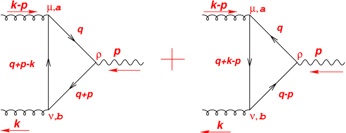
FIG. 2.: The two gluon photon effective vertex as the sum of two diagrams with quark number running in opposite directions.

Let us now focus our attention on the diagrams of Fig. 2. Such a process does not exist at zero temperature or even at finite temperature and zero density. At finite density this may lead to a new source of dilepton or photon production. In this section we obtain general expressions for this diagram.

We sum the Matsubara frequencies using Pisarski’s non-covariant method [11] (Our notation is however different from that in [11] and is explained in Appendix A.). In this method, propagators may be expanded as follows,

$$\frac{1}{q^{2}}=\tilde{\Delta}(q)=(-i)\int_{0}^{-i\beta}dx_{2}^{0}\;e^{-i(q^{0}-\mu)x_{2}^{0}}\;\tilde{\Delta}^{\prime}(|\vec{q}|,-x_{2}^{0}),$$ (10)

where

$\displaystyle\tilde{\Delta}^{\prime}(|\vec{q}|,-x_{2}^{0})=\frac{1}{2E_{q}}\sum_{s_{2}}\tilde{f}_{s_{2}}^{\prime}(E_{q},s_{2}\mu)e^{-is_{2}(E_{q}+s_{2}\mu)x_{2}^{0}},$

where $\tilde{f}^{\prime}_{+}=1-\tilde{n}(E+\mu)\;,\tilde{f}^{\prime}_{-}=-\tilde{n}(E-\mu)$, and $\tilde{n}$ is the Fermi-Dirac distribution function. Then,

$$\frac{1}{(q+p-k)^{2}} = \tilde{\Delta}(q+p-k)$$ (11)

$$= (-i)\int_{0}^{-i\beta}dx_{1}^{0}\;e^{i(q^{0}+p^{0}-k^{0}-\mu)x_{1}^{0}}\;\Delta(|\vec{q}+\vec{p}-\vec{k}|,x_{1}^{0})$$ (12)

$\displaystyle\tilde{\Delta}(|\vec{q}+\vec{p}-\vec{k}|,x_{1}^{0})=\frac{1}{2E_{q+p-k}}\sum_{s_{1}}\tilde{f}_{s_{1}}(E_{q+p-k},s_{1}\mu)e^{-is_{1}(E_{q+p-k}-s_{1}\mu)x_{1}^{0}},$

where $\tilde{f}_{+}=1-\tilde{n}(E-\mu)\;,\tilde{f}_{-}=-\tilde{n}(E+\mu)$. For the last propagator, we may write

$$\frac{1}{(q+p)^{2}} = \tilde{\Delta}(q+p)$$ (13)

$$= (-i)\int_{0}^{-i\beta}dx_{3}^{0}\;e^{i(q^{0}+p^{0}-\mu)x_{3}^{0}}\;\tilde{\Delta}(|\vec{q}+\vec{p}|,x_{3}^{0})$$ (14)

with

$\displaystyle\tilde{\Delta}(|\vec{q}+\vec{p}|,x_{3}^{0})=\frac{1}{2E_{q+p}}\sum_{s_{3}}\tilde{f}_{s_{3}}(E_{q+p},s_{3}\mu)e^{-is_{3}(E_{q+p}-s_{3}\mu)x_{3}^{0}}.$

In the above three equations $s_{1},s_{2},s_{3}$ are sign factors which are either +1 or -1, and $q^{0}\rightarrow i(\frac{\partial}{\partial x_{2}^{0}}-i\mu)$. We substitute the above three equations in Eq. (4) and add the two diagrams. Now, one may simply perform the Matsubara sum to obtain a delta function over the times (see Appendix B). Using the delta function we may evaluate the remaining time integrations to give the full expression for this vertex as (see Appendix B)

$${\mathcal{T}}^{\mu\rho\nu}=\int\frac{d^{3}q}{(2\pi)^{3}}\frac{\delta^{ab}}{2}eg^{2}\sum_{s_{1}s_{2}s_{3}}Tr[\gamma^{\mu}\gamma^{\beta}\gamma^{\rho}\gamma^{\delta}\gamma^{\nu}\gamma^{\alpha}]\frac{\widehat{(q+p-k)}_{s_{1},\alpha}\hat{q}_{s_{2},\beta}\widehat{(q+p)}_{s_{3},\delta}}{p^{0}+s_{2}E_{q}-s_{3}E_{q+p}}$$ (17)

$$\!\!\!\!\!\!\!\!\!\!\!\!\!\!\!\!\!\!\!\!\!\!\left[s_{2}\frac{s_{3}(\tilde{n}(E_{q+p-k}+s_{1}\mu)-\tilde{n}(E_{q+p-k}-s_{1}\mu))-s_{1}(\tilde{n}(E_{q+p}+s_{3}\mu)-\tilde{n}(E_{q+p}-s_{3}\mu))}{k^{0}+s_{1}E_{q+p-k}-s_{3}E_{q+p}}\right.$$

$$\!\!\!\!\!\!\!\!\!\!\!\!\!\!\!\!\!\!\!\!\!\!\!\!\!\left.\mbox{}-s_{3}\frac{s_{2}(\tilde{n}(E_{q+p-k}+s_{1}\mu)-\tilde{n}(E_{q+p-k}-s_{1}\mu))-s_{1}(\tilde{n}(E_{q}+s_{2}\mu)-\tilde{n}(E_{q}-s_{2}\mu))}{k^{0}-p^{0}+s_{1}E_{q+p-k}-s_{2}E_{q}}\right].$$

In the above equation $E_{q-k}=\sqrt{|\vec{q}|^{2}+|\vec{k}|^{2}-2|\vec{q}||\vec{k}|\cos{\theta}}$, where $\cos{\theta}$ is the angle between $\vec{q}$ and $\vec{k}$. While in the numerator

$\displaystyle\hat{q}_{s_{2}}=(s_{2},\sin{\theta}\cos{\phi},\sin{\theta}\sin{\phi},\cos{\theta}),$

and

$\displaystyle\widehat{(q-k)}_{s_{1}}=\Bigg{(}s_{1},\frac{q\sin{\theta}\cos{\phi}}{|\vec{q}-\vec{k}|},\frac{q\sin{\theta}\sin{\phi}}{|\vec{q}-\vec{k}|},\frac{q\cos{\theta}-k}{|\vec{q}-\vec{k}|}\Bigg{)}.$

Up to this point no approximations have been made. Completing the remaining angular integrations will lead to the expression for the effective vertex with arbitrary momenta $k,p$. This, however, turns out to be rather difficult. Even in the Hard Thermal Loop (HTL) approximation, evaluation of similar three point loops for arbitrary three momentum $\vec{p}$ is a difficult problem [13]. For the HTL approximation to be valid, the temperature should be high, and the momentum in the outer legs should be low. Predicted, initial temperatures at RHIC and LHC range from 300 to 800 MeV [14, 15]. Dileptons from the plasma are predicted to become important in the intermediate mass regime (1-3 GeV)[4]. In this region of parameter space the HTL approximation obviously does not apply . Hence we do not make this approximation in this work. Furthermore, in the interest of technical simplicity, we proceed to evaluate the above diagram in the limit of the photon three momentum $\vec{p}=0$, i.e., for dilepton pairs produced back-to-back.

In this limit the expression for the effective vertex reduces to

$${\mathcal{T}}^{\mu\rho\nu} = \int\frac{d^{3}q}{(2\pi)^{3}}\frac{\delta^{ab}}{2}eg^{2}\sum_{s_{1}s_{2}s_{3}}Tr[\gamma^{\mu}\gamma^{\beta}\gamma^{\rho}\gamma^{\delta}\gamma^{\nu}\gamma^{\alpha}]\frac{\widehat{(q-k)}_{s_{1},\alpha}\hat{q}_{s_{2},\beta}\hat{q}_{s_{3},\delta}}{p^{0}+s_{2}E_{q}-s_{3}E_{q}}$$ (19)

$$\!\!\!\!\!\!\!\!\!\!\!\!\!\!\!\!\!\!\!\!\!\!\left[s_{2}\frac{s_{3}\Delta\tilde{n}(E_{q-k},s_{1}\mu)-s_{1}\Delta\tilde{n}(E_{q},s_{3}\mu)}{k^{0}+s_{1}E_{q-k}-s_{3}E_{q}}-s_{3}\frac{s_{2}\Delta\tilde{n}(E_{q-k},s_{1}\mu)-s_{1}\Delta\tilde{n}(E_{q},s_{2}\mu)}{k^{0}-p^{0}+s_{1}E_{q-k}-s_{2}E_{q}}\right].$$

In the above, the notation $\Delta\tilde{n}(E,s\mu)=\tilde{n}(E+s\mu)-\tilde{n}(E-s\mu)$) is introduced. The $\Delta\tilde{n}$’s quantify the effect of a finite chemical potential, as they represent the difference between the distribution functions of a quark and its antiquark. If $\mu\rightarrow 0$, all the $\Delta\tilde{n}$’s go to zero and so does the entire expression. Noting that $s_{2}\Delta\tilde{n}(E_{q},s_{3}\mu)=s_{3}\Delta\tilde{n}(E_{q},s_{2}\mu)$, we may add up the two terms in the integrand to give,

$${\mathcal{T}}^{\mu\rho\nu} = \int\frac{d^{3}q}{(2\pi)^{3}}\frac{\delta^{ab}}{2}eg^{2}\sum_{s_{1}s_{2}s_{3}}Tr[\gamma^{\mu}\gamma^{\beta}\gamma^{\rho}\gamma^{\delta}\gamma^{\nu}\gamma^{\alpha}]\widehat{(q-k)}_{s_{1},\alpha}\hat{q}_{s_{2},\beta}\hat{q}_{s_{3},\delta}$$ (21)

$$\left[\frac{s_{2}s_{1}\Delta\tilde{n}(E_{q},s_{3}\mu)-s_{2}s_{3}\Delta\tilde{n}(E_{q-k},s_{1}\mu)}{(k^{0}+s_{1}E_{q-k}-s_{3}E_{q})(k^{0}-p^{0}+s_{1}E_{q-k}-s_{2}E_{q})}\right].$$

Note that the integrand of the above expression for the vertex has factorized into a function of the form $f_{1}(k_{0})f_{2}(p_{0}-k_{0})$. This result will become important in the eventual evaluation of the photon self-energy in the subsequent sections.

We note that the sole $\phi$ dependence is in the numerator. This allows us to integrate out the $\phi$ dependence. The presence of the Lorentz indices $\alpha,\beta,\gamma$ indicate that Eq. (21) actually contains 64 separate terms. The $Tr[\gamma^{\mu}\gamma^{\beta}\gamma^{\rho}\gamma^{\delta}\gamma^{\nu}\gamma^{\alpha}]$ combines these into 64 other terms. Ignoring the trace part, the rest of the formula is found to contain only 20 nonzero terms (see Appendix C). Of these 20 terms we observe many to be interdependent. There are at most 8 independent terms (see Appendix C).

To perform the $\theta$ integration we shift $\vec{q}$ in the second term of the integrand of Eq. (21) to give

$${\mathcal{T}}^{\mu\rho\nu} = \int\frac{dqq^{2}d\theta d\phi\sin{\theta}}{(2\pi)^{3}}\frac{\delta^{ab}}{2}eg^{2}\sum_{s_{1}s_{2}s_{3}}Tr[\gamma^{\mu}\gamma^{\beta}\gamma^{\rho}\gamma^{\delta}\gamma^{\nu}\gamma^{\alpha}]$$ (24)

$$\left[\widehat{(q-k)}_{s_{1},\alpha}\hat{q}_{s_{2},\beta}\hat{q}_{s_{3},\delta}\frac{s_{2}s_{1}\Delta\tilde{n}(E_{q},s_{3}\mu)}{(k^{0}+s_{1}E_{q-k}-s_{3}E_{q})(k^{0}-p^{0}+s_{1}E_{q-k}-s_{2}E_{q})}\right.$$

$$\mbox{}-\left.\hat{q}_{s_{1},\alpha}\widehat{(q+k)}_{s_{2},\beta}\widehat{(q+k)}_{s_{3},\delta}\frac{s_{2}s_{3}\Delta\tilde{n}(E_{q},s_{1}\mu)}{(k^{0}+s_{1}E_{q}-s_{3}E_{q+k})(k^{0}-p^{0}+s_{1}E_{q}-s_{2}E_{q+k})}\right].$$

The resulting $(\theta,\phi)$ integration now becomes rather simple.

IV THE PHOTON SELF-ENERGY AND ITS IMAGINARY PART

We are now in a position to calculate the contribution made by the diagram of Fig. 2 to the dilepton spectrum emanating from a quark gluon plasma. To achieve this aim we choose to calculate the imaginary part of the photon self-energy as represented by the diagram of Fig. 3. In the previous section we wrote down expressions for ${\mathcal{T}}^{\mu\rho\nu}(k-p,k;p)$. To write down the expression for the full self-energy we also need expressions for ${\mathcal{T}}^{\zeta\rho\eta}(k,k-p;-p)$. A simple analysis consisting of essentially reversing the direction of the internal momentum $\vec{q}$ leads us to the result that ${\mathcal{T}}^{\zeta\rho\eta}(k,k-p;-p)={\mathcal{T}}^{\eta\rho\zeta}(k-p,k;p)$.

We may write down the full expression for the photon self-energy as

$$\Pi^{\rho}_{\rho}=\frac{1}{\beta}\sum_{k^{0}}\int\frac{d^{3}k}{(2\pi)^{3}}{\mathcal{D}}_{\eta\mu}(k){\mathcal{T}}^{\mu\rho\nu}(k-p,k;p){\mathcal{D}}_{\nu\zeta}(k-p){\mathcal{T}}^{\zeta\rho\eta}(k,k-p;-p).$$ (25)

FIG. 3.: The Full photon self-energy at three loop and the cut that is evaluated in this paper.

We perform this calculation in the Feynman gauge for the gluons, thus

$${\mathcal{D}}_{\eta\mu}(k)=\frac{g_{\eta\mu}}{k^{2}}.$$ (26)

We calculate in the limit of photon three momentum $\vec{p}=0$. We now shift $k\rightarrow k+p$. Notice that, in the limit $\vec{p}=0$, this only implies shifting $k^{0}$ by $p^{0}$. This is followed by switching $k^{0}\rightarrow-k^{0}$. Note that neither of these operations has any effect on the full nature of the integral as $k^{0}$ is summed over all even discrete frequencies. With this we now obtain the full self-energy as

$$\Pi^{\rho}_{\rho} = e^{2}g^{4}\frac{32}{9}{\mathcal{C}}_{\alpha\beta\gamma}^{\alpha^{\prime}\beta^{\prime}\gamma^{\prime}}\int\frac{d^{3}kd^{3}qdq^{\prime 3}}{(2\pi)^{9}}\frac{1}{\beta}\sum_{k^{0}}\sum_{s_{1}s_{2}s_{3}s_{1}^{\prime}s_{2}^{\prime}s_{3}^{\prime}}\frac{1}{(k^{0})^{2}-k^{2}}\frac{1}{(p^{0}-k^{0})^{2}-k^{2}}$$ (29)

$$\times\left[\frac{\widehat{(q-k)}_{s_{1}}^{\alpha}\hat{q}_{s_{2}}^{\beta}\hat{q}_{s_{3}}^{\gamma}\{s_{2}s_{1}\Delta\tilde{n}(E_{q},s_{3}\mu)-s_{2}s_{3}\Delta\tilde{n}(E_{q-k},s_{1}\mu)\}}{(-k^{0}+p^{0}+s_{1}E_{q-k}-s_{3}E_{q})(-k^{0}+s_{1}E_{q-k}-s_{2}E_{q})}\right]$$

$$\times\left[\frac{\widehat{(q^{\prime}-k)}_{s_{1}^{\prime},\alpha^{\prime}}\hat{q^{\prime}}_{s_{2}^{\prime},\beta^{\prime}}\hat{q^{\prime}}_{s_{3}^{\prime},\gamma^{\prime}}\{s_{2}^{\prime}s_{1}^{\prime}\Delta\tilde{n}(E_{q^{\prime}},s_{3}^{\prime}\mu)-s_{2}^{\prime}s_{3}^{\prime}\Delta\tilde{n}(E_{q^{\prime}-k},s_{1}^{\prime}\mu)\}}{(-k^{0}+p^{0}+s_{1}^{\prime}E_{q^{\prime}-k}-s_{3}^{\prime}E_{q^{\prime}})(-k^{0}+s_{1}^{\prime}E_{q^{\prime}-k}-s_{2}^{\prime}E_{q^{\prime}})}\right].$$

Where the multiplicative factor ${\mathcal{C}}_{\alpha\beta\gamma}^{\alpha^{\prime}\beta^{\prime}\gamma^{\prime}}$ is the result of the contraction of Lorentz indices appearing in the two traces of 6 $\gamma$ matrices and the intervening factors of the metric. In the above expression, we have also assumed the presence of three massless flavours of quarks. For simplicity the chemical potential is assumed to be the same for all three flavours. In order to calculate the differential rate of back to back dileptons we need to evaluate the imaginary part of this diagram. This may be obtained in two ways: the conventional method [12] involves converting the sum over discrete frequencies into a contour integral, followed by evaluation of the contour integral by summing over its residues and then looking for poles and branch cuts in the final expression in terms of $p^{0}$ by analytically continuing $p^{0}$ onto the real axis. Ten years ago Braaten, Pisarski, and Yuan presented an identity [16] which elegantly achieved the end result of this procedure for a fermionic Matsubara frequency $k^{0}$ . In the following we will refer to this formula as the BPY formula. It is given, generally, in terms of products of arbitrary functions of discrete imaginary frequencies as (for completeness, a brief proof of the BPY formula for a Bosonic frequency $k^{0}$ in terms of the method of [12] is presented in appendix D)

$$\mbox{Disc}T\sum_{k^{0}}f_{1}(k^{0})f_{2}(p^{0}-k^{0}) = 2\pi i(1-e^{E/T})\int_{-\infty}^{+\infty}d\omega\int_{-\infty}^{+\infty}d\omega^{\prime}$$ (31)

$$n(\omega)n(\omega^{\prime})\delta(E-\omega-\omega^{\prime})\rho_{1}(\omega)\rho_{2}(\omega^{\prime}),$$

where $\rho_{1}(\omega)$,$\rho_{2}(\omega^{\prime})$ are the spectral densities of $f_{1}(z)$,$f_{2}(z)$. Note that Eq. (29) is precisely in the form required by Eq. (31), with

$$f_{1}(k^{0}) = \frac{1}{[k^{0}-(s_{1}x-s_{2}q)][k_{0}-(s_{1}^{\prime}x^{\prime}-s_{2}^{\prime}q^{\prime})][(k^{0})^{2}-k^{2}]}$$ (32)

$$f_{2}(p^{0}-k^{0}) = \frac{1}{[p^{0}-k^{0}-(s_{1}x-s_{3}q)][k_{0}-(s_{1}^{\prime}x^{\prime}-s_{3}^{\prime}q^{\prime})][(p^{0}-k^{0})^{2}-k^{2}]},$$ (33)

where, for brevity we have $x(x^{\prime})=E_{q-k}(E_{q^{\prime}-k})$ and $q(q^{\prime})=E_{q}(E_{q^{\prime}})$. From here, one may write down the spectral densities of the two functions by mere inspection:

$$\rho_{1}(\omega) = \delta(\omega-k)\mbox{Res}[f_{1}(\omega=k)]+\delta(\omega+k)\mbox{Res}[f_{1}(\omega=-k)]$$ (34)

$$+ \delta(\omega-(s_{1}x-s_{2}q))\mbox{Res}[f_{1}(\omega=s_{1}x-s_{2}q)]$$ (35)

$$+ \delta(\omega-(s_{1}^{\prime}x^{\prime}-s_{2}^{\prime}q^{\prime}))\mbox{Res}[f_{1}(\omega=s_{1}^{\prime}x^{\prime}-s_{2}^{\prime}q^{\prime})]$$ (36)

$$\rho_{2}(\omega^{\prime}) = \delta(\omega^{\prime}-k)\mbox{Res}[f_{1}(\omega^{\prime}=k)]+\delta(\omega^{\prime}+k)\mbox{Res}[f_{1}(\omega^{\prime}=-k)]$$ (37)

$$+ \delta(\omega^{\prime}-(s_{1}x-s_{3}q))\mbox{Res}[f_{1}(\omega^{\prime}=s_{1}x-s_{3}q)]$$ (38)

$$+ \delta(\omega^{\prime}-(s_{1}^{\prime}x^{\prime}-s_{3}^{\prime}q^{\prime}))\mbox{Res}[f_{1}(\omega^{\prime}=s_{1}^{\prime}x^{\prime}-s_{3}^{\prime}q^{\prime})].$$ (39)

In the above equation Res$[f(\omega)]$ stands for the residue of the function $f$ at $\omega$. In the language of BPY [16], the first two terms of the two spectral densities are the pole terms. The next two are the cut terms as they contain $q$ and $x$; variables which will get integrated over before the $k$ integration. There are, of course, other multiplicative factors which depend on $k,x,\mbox{ and }q$ which have not been expressly written down in Eq. (39).

We now take the product of the two spectral densities as given in Eq. (39). Each combination of delta functions gives us a different cut of the diagram. For instance combining any of the pole terms from the two spectral densities gives us the cut shown in Fig. 3 (and thus, the resulting cross section for the second diagram ). This represents the process of gluon-gluon to $\mbox{e}^{+}\mbox{e}^{-}$. This is a new process which to our knowledge has never been discussed before. The other possible cuts represent essentially finite density contributions to other known processes of dilepton production: two loop contributions to $q\bar{q}\rightarrow\gamma^{*}$, one loop contributions to $qg\rightarrow q\gamma^{*}$, and $qq\rightarrow qq\gamma^{*}$.

In the following we focus exclusively on the first process i.e., $gg\rightarrow\gamma^{*}$. The reasons for this are twofold. The first is the fact that this process is unique and resembles nothing at zero density; all the other processes are extra contributions to processes which are known and have been calculated up to two-loop level at finite temperature and zero density [17, 18, 19]. Secondly, all the other diagrams have at least one internal gluon line which is weighted by Bose Einstein statistics, and hence, these diagrams will display infrared divergence. To cure this divergence one can replace the bare gluon propagator with a resumed HTL propagator. These rather involved calculations deserve a separate treatment. In contrast, all the internal lines of the first process are fermions and hence show no infrared divergence.

V THE CALCULATION

We now apply the BPY formula with only the pole-pole terms from Eq. (39). The various delta function combinations that are encountered can be schematically written as

$$\delta(E-\omega-\omega^{\prime})\rho_{1}\rho_{2} = \delta(E-\omega-\omega^{\prime})\Bigg{[}\delta(\omega-k)\mbox{Res}[f_{1}(\omega=k)]\delta(\omega^{\prime}-k)\mbox{Res}[f_{2}(\omega^{\prime}=k)]$$ (40)

$$+ \delta(\omega-k)\mbox{Res}[f_{1}(\omega=k)]\delta(\omega^{\prime}+k)\mbox{Res}[f_{2}(\omega^{\prime}=-k)]$$ (41)

$$+ \delta(\omega+k)\mbox{Res}[f_{1}(\omega=-k)]\delta(\omega^{\prime}-k)\mbox{Res}[f_{2}(\omega^{\prime}=k)]$$ (42)

$$+ \delta(\omega+k)\mbox{Res}[f_{1}(\omega=-k)]\delta(\omega^{\prime}+k)\mbox{Res}[f_{2}(\omega^{\prime}=-k)]\Bigg{]}.$$ (43)

Note that only the first term (i.e., gluon-gluon annihilation) survives. In this term $\omega=\omega^{\prime}=k=E/2$. Thus, this contribution to the discontinuity of the photon self-energy may be given as

$$\mbox{Disc}[\Pi^{\rho}_{\rho}] = e^{2}g^{4}\frac{64}{9}\pi i(1-e^{E/T}){\mathcal{C}}_{\alpha\beta\gamma}^{\alpha^{\prime}\beta^{\prime}\gamma^{\prime}}\int\frac{4\pi k^{2}dqdq^{\prime}q^{2}q^{\prime 2}d\theta d\theta^{\prime}\sin{\theta}\sin{\theta^{\prime}}}{(2\pi)^{7}}\sum_{s_{1}s_{2}s_{3}s_{1}^{\prime}s_{2}^{\prime}s_{3}^{\prime}}\frac{1}{4k^{2}}$$ (46)

$$\times\left[\frac{\widehat{(q-k)}_{s_{1}}^{\alpha}\hat{q}_{s_{2}}^{\beta}\hat{q}_{s_{3}}^{\gamma}\{s_{2}s_{1}\Delta\tilde{n}(E_{q},s_{3}\mu)-s_{2}s_{3}\Delta\tilde{n}(E_{q-k},s_{1}\mu)\}}{(k+(s_{1}E_{q-k}-s_{3}E_{q}))(k-(s_{1}E_{q-k}-s_{2}E_{q}))}\right]$$

$$\times\left[\frac{\widehat{(q^{\prime}-k)}_{s_{1}^{\prime},\alpha^{\prime}}\hat{q^{\prime}}_{s_{2}^{\prime},\beta^{\prime}}\hat{q^{\prime}}_{s_{3}^{\prime},\gamma^{\prime}}\{s_{2}^{\prime}s_{1}^{\prime}\Delta\tilde{n}(E_{q^{\prime}},s_{3}^{\prime}\mu)-s_{2}^{\prime}s_{3}^{\prime}\Delta\tilde{n}(E_{q^{\prime}-k},s_{1}^{\prime}\mu)\}}{(k+(s_{1}^{\prime}E_{q^{\prime}-k}-s_{3}^{\prime}E_{q^{\prime}}))(k-(s_{1}^{\prime}E_{q^{\prime}-k}-s_{2}^{\prime}E_{q^{\prime}}))}\right].$$

As stated before, the multiplicative factor ${\mathcal{C}}_{\alpha\beta\gamma}^{\alpha^{\prime}\beta^{\prime}\gamma^{\prime}}$ is the result of the contraction of Lorentz indices appearing in the two traces of 6 $\gamma$ matrices and the intervening factors of the metric. Essentially, this serves the purpose of the average over initial spins. We basically now have four terms to integrate (there is no mixed term between ($q,\theta$) and ($q^{\prime},\theta^{\prime}$) ). Each term is classified by its fermionic distribution function. Now we may shift the variable $\vec{q}\rightarrow\vec{q}+\vec{k}$ in the second and fourth fermionic distribution functions, and the $\theta$ and $\theta^{\prime}$ integrals become simple and can be done analytically. The two $q$ and $q^{\prime}$ integrations are then done numerically.

The differential production rate for pairs of massless leptons with total energy $E$ and and total momentum $\vec{p}=0$ is given in terms of the discontinuity in the photon self-energy as [20]

$$\frac{dW}{dEd^{3}p}(\vec{p}=0)=\frac{\alpha}{12\pi^{3}}\frac{1}{E^{2}}\frac{1}{1-e^{E/T}}\frac{1}{2\pi i}\mbox{Disc}\Pi_{\rho}^{\rho}(0).$$ (47)

Where $\alpha$ is the electromagnetic coupling constant. The rate of production of a hard lepton pair with total momentum $\vec{p}=0$ at one-loop order in the photon self-energy (i.e., the Born term ) is given as

$$\frac{dW}{dEd^{3}p}(\vec{p}=0)=\frac{\alpha^{2}}{6\pi^{4}}\tilde{n}(E/2-\mu)\tilde{n}(E/2+\mu).$$ (48)

As mentioned before, initial temperatures of the plasma formed at RHIC and LHC have been predicted to lie in the range from 300-800 MeV [14, 15]. For this exploratory calculation we use a conservative estimate of $T=400\mbox{ MeV}$. To evaluate the effect of a finite chemical potential we perform the calculation with two extreme values of chemical potential $\mu=0.1T$ (Fig. 4) and $\mu=0.5T$(Fig. 5) [21]. The calculation, as stated before, is performed for three massless flavours of quarks. In this case the strong coupling constant is (see [19])

$$\alpha_{s}(T)=\frac{6\pi}{27ln(T/50MeV)}.$$ (49)

The differential rate for the production of dileptons with an invariant mass from 0.5 to $2.5\mbox{ GeV}$ is presented. On purpose, we avoid regions where the gluons become very soft. In the figures, the dashed line is the rate from tree level $q\bar{q}$ (Eq. (48)); the solid line is that from the process $gg\rightarrow e^{+}e^{-}$. We note that in both cases the gluon-gluon process dominates at low energy and dies out at higher energy leaving the $q\bar{q}$ process dominant at higher energy.

FIG. 4.: The differential production rate of back to back dileptons from two processes. Invariant mass runs from 0.5 GeV to 2.5 GeV. The dashed line represents the contribution from the process $q\bar{q}\rightarrow e^{+}e^{-}$. The solid line corresponds to the process $gg\rightarrow e^{+}e^{-}$. Temperature is 400 MeV. Quark chemical potential is 0.1T.

FIG. 5.: Same as Fig. 4 but with $\mu=0.5T$

VI DISCUSSIONS AND CONCLUSION

In this paper we have performed a calculation to estimate the effects of a non-zero quark chemical potential on the intermediate mass dilepton spectra. We have found that a new set of diagrams may become important at finite temperature and finite density. These diagrams lead to a new contribution to the photon self-energy at the 3-loop order. There are various cuts to this diagram. Most of these result in finite density contributions, and/or higher order excess contributions to well known processes. One of the cuts however represents an entirely new process. The contribution of this diagram to the differential production rate of back-to-back (or $\vec{p}=0$) dileptons is estimated. This is then compared with the contribution emanating from the tree level process of $q\bar{q}$ annihilation. The rate from this new process is found to be larger than the simple tree level rate by orders of magnitude between a dilepton invariant mass of 0.5 to 1.5 GeV. The reasons for this large magnitude are many. The gluon-gluon diagram is enhanced by the Bose-Einstein distribution function of the gluons. Also, at lower energy the $\Delta n$ factors which represent the difference between the quark and antiquark distribution functions are comparable in size to the distribution functions themselves. There is, also, enhancement from the larger color factors of the gluons. One also notes that as the energy (invariant mass) is increased, the difference between the two distribution functions ($\Delta n$) decreases rapidly, i.e., as higher energies the distributions of quarks and antiquarks becomes less sensitive to the chemical potential. This is the main reason behind the sharp drop of the differential rate compared to the differential rate from quark-antiquark annihilation.

These results demonstrate the importance of these finite $\mu$ processes on the dilepton spectra emanating from a quark gluon plasma with a quark-antiquark asymmetry. It is simple to note that this diagram is most sensitive to gluon number. The early stages of the plasma have been predicted to be gluon dominated [22]. The contribution from this diagram should clearly shine in such an environment.

The treatment in this rather exploratory work should, and will, be improved upon. Our goal here was simply to establish the existence of a signal. One may have desired, for example, that the calculation be extended to arbitrary $\vec{p}$. However, similar extensions, even in the HTL approximation, are known to be rather involved [13]. There are also the other diagrams which have yet to be computed. These however suffer from the defect of having an internal boson line which will show an infrared divergence. This bare propagator will have to replaced by a resumed HTL propagator, in the event that the momentum flowing through it becomes very small. These aspects, along with others, will be addressed elsewhere.

VII ACKNOWLEDGMENT

The authors wish to thank Y. Aghababaie, S. Das Gupta , F. Gelis, S. Jeon, D. Kharzeev, C. S. Lam and G. D. Mahlon for helpful discussions. A.M. acknowledges the generous support provided to him by McGill University through the Alexander McFee fellowship, the Hydro-Quebec fellowship and the Neil Croll award. This work was supported in part by the Natural Sciences and Engineering Research Council of Canada and by le fonds pour la Formation de Chercheurs et l’aide à la Recherche du Québec.

VIII APPENDIX A

Notation.

Our notation is categorized by the explicit presence of an apparent Minkowski time $x^{0}=-i\tau$ and a momentum $q^{0}=i(2n+1)\pi T+\mu$. Our metric is $(1,-1,-1,-1)$. For the case of zero chemical potential our bosonic propagators have the same appearance as at zero temperature, i.e.,

$$i\Delta(q)=\frac{i}{(q^{0})^{2}-|q|^{2}}.$$ (50)

The Feynman rules are also the same as at zero temperature, with the understanding that we replace the zeroth component of the momentum by Eq. (5) for a fermion and by an even frequency in the case of a boson. One may, in the case of zero chemical potential, relate this to the familiar case of reference [11] by noting that

$$\Delta(q)=\frac{1}{(q^{0})^{2}-|q|^{2}}=\frac{-1}{(\omega_{n})^{2}+|q|^{2}}=-\Delta_{E}(\omega_{n},q),$$ (51)

where $\Delta_{E}(\omega_{n},q)$ is the familiar Euclidean propagator presented in the literature ([11],[12]). One may immediately surmise the form of the non-covariant propagator $\Delta(|\vec{q}|,x^{0})$, the Fourier transform of which is the covariant propagator.

$$\Delta(q,q^{0}) = -\int_{0}^{\beta}d\tau e^{-i\omega_{n}\tau}\Delta_{E}(|\vec{q}|,\tau)$$ (52)

$$= -i\int_{0}^{-i\beta}dx^{0}e^{iq^{0}x^{0}}\Delta_{E}(|\vec{q}|,\tau)$$ (53)

$$= -i\int_{0}^{-i\beta}dx^{0}e^{iq^{0}x^{0}}\Delta(|\vec{q}|,x^{0}).$$ (54)

In the presence of a finite chemical potential our full fermionic propagators become

$$S(q,q^{0})=(\gamma^{\mu}q_{\mu})(-i)\int_{0}^{-i\beta}dx^{0}e^{i(q^{0}-\mu)x^{0}}\Delta_{\mu}(|\vec{q}|,x^{0}),$$ (55)

where,

$$\Delta_{\mu}(|\vec{q}|,x^{0})=\frac{1}{2E_{q}}\sum_{s}f_{s}(E_{q}-s\mu)e^{-isx^{0}(E_{q}-s\mu)}.$$ (56)

In the above two equations $q^{0}=i(2n+1)\pi T+\mu$.

IX APPENDIX. B

Derivation of Eq. 17.

As stated in section III we start by substituting Eqs. (10,12, 14) in Eq. (4). Substituting in the first diagram we get,

$$T^{\mu\rho\nu} = \frac{1}{\beta}\sum_{n}\int\frac{d^{3}q}{2\pi^{3}}\frac{\delta_{ab}}{2}Tr[6\gamma]\sum_{s_{1},s_{2},s_{3}}\frac{(q+p-k)_{s_{1}\alpha}q_{-s_{2}\beta}(q+p)_{s_{3}\gamma}}{8E_{q+p-k}E_{q}E_{q+p}}\Bigg{[}\int_{0}^{-i\beta}dx_{1}^{0}dx_{2}^{0}dx_{3}^{0}$$ (60)

$$e^{-i(q^{0}-\mu)x_{2}^{0}}e^{i(q^{0}+p^{0}-k^{0}-\mu)x_{1}^{0}}e^{i(q^{0}+k^{0}-\mu)x_{3}^{0}}$$

$$\tilde{f}_{s_{1}}(E_{q+p-k},s_{1}\mu)\tilde{f}_{s_{2}}^{\prime}(E_{q},s_{2}\mu)\tilde{f}_{s_{3}}(E_{q+p},s_{3}\mu)$$

$$e^{-is_{2}(E_{q}+s_{2}\mu)x_{2}^{0}}e^{-is_{1}(E_{q+p-k}+s_{1}\mu)x_{1}^{0}}e^{-is_{3}(E_{q+p}+s_{3}\mu)x_{3}^{0}}\Bigg{]}.$$

In our formalism $x^{0}=-i\tau$. Also, in Eq. (4) the zeroth components of the momenta are replaced by time derivatives e.g.,

$\displaystyle q_{0}=i\frac{d}{dx_{2}^{0}}+\mu,$

with the derivative acting on the $e^{-i(q^{0}-\mu)x_{2}^{0}}$. We then perform a by parts integration w.r.t. $x_{2}^{0}$, after which the derivative acts on the $e^{-is_{2}(E_{q}+s_{2}\mu)x_{2}^{0}}$ term. After some algebraic manipulation and using the definition that $q_{s_{2}0}=s_{2}E_{q}$, we obtain Eq. (LABEL:appB). We have the identity

$$\frac{1}{\beta}\sum e^{iq^{0}(x_{1}^{0}-x_{2}^{0}+x_{3}^{0})}=\delta(\tau_{1}-\tau_{2}+\tau_{3})+(-1)\delta(\tau_{1}-\tau_{2}+\tau_{3}-\beta).$$ (62)

Using the above identity we perform the Matsubara sum and then evaluate one of the $\tau$ integrals using the two delta functions. Noting that $e^{p^{0}\beta}=1$ we get

$$T^{\mu\rho\nu} = \int\frac{d^{3}q}{2\pi^{3}}\frac{\delta_{ab}}{2}Tr[6\gamma]\sum_{s_{1},s_{2},s_{3}}\frac{(q+p-k)_{s_{1}\alpha}q_{-s_{2}\beta}(q+p)_{s_{3}\gamma}}{8E_{q+p-k}E_{q}E_{q+p}}\int_{0}^{-i\beta}dx_{1}^{0}dx_{2}^{0}$$ (65)

$$e^{i(p^{0})x_{2}^{0}}e^{-i(k^{0})x_{1}^{0}}\tilde{f}_{s_{1}}(E_{q+p-k},s_{1}\mu)\tilde{f}_{s_{2}}^{\prime}(E_{q},s_{2}\mu)\tilde{f}_{s_{3}}(E_{q+p},s_{3}\mu)$$

$$e^{-ix_{2}^{0}(s_{2}E_{q}+s_{3}E_{q+p})}e^{-ix_{1}^{0}(s_{1}E_{q+p-k}-s_{3}E_{q+p})}\Bigg{[}\Theta(\tau_{2}-\tau_{1})-\Theta(\tau_{1}-\tau_{2})e^{\beta(-s_{3}E_{q+p}+\mu)}\Bigg{]}.$$

Noting that $e^{\beta(-s_{3}E_{q+p}+\mu)}=-\frac{\tilde{f}_{-s_{3}}^{\prime}(E_{q+p},s_{3}\mu)}{\tilde{f}_{s_{3}}(E_{q+p},s_{3}\mu)}$ we may integrate $x_{2}^{0}$ making explicit use of the two Heaviside theta functions to obtain,

$$T^{\mu\rho\nu} = \int\frac{d^{3}q}{2\pi^{3}}\frac{\delta_{ab}}{2}Tr[6\gamma]\sum_{s_{1},s_{2},s_{3}}\frac{(q+p-k)_{s_{1}\alpha}q_{-s_{2}\beta}(q+p)_{s_{3}\gamma}}{8E_{q+p-k}E_{q}E_{q+p}}\int_{0}^{-i\beta}dx_{1}^{0}$$ (69)

$$e^{-ix_{1}^{0}(k^{0}+s_{1}E_{q+p-k}-s_{3}E_{3})}\tilde{f}_{s_{1}}(E_{q+p-k},s_{1}\mu)\tilde{f}_{s_{2}}^{\prime}(E_{q},s_{2}\mu)$$

$$\Bigg{[}\tilde{f}_{s_{3}}(E_{q+p},s_{3}\mu)\frac{e^{i(-i\beta)(p^{0}-s_{2}E_{q}-s_{3}E_{q+p})}-e^{i(x_{1}^{0})(p^{0}-s_{2}E_{q}-s_{3}E_{q+p})}}{i(p^{0}-s_{2}E_{q}-s_{3}E_{q+p})}$$

$$\mbox{}+\tilde{f}_{-s_{3}}^{\prime}(E_{q+p},s_{3}\mu)\frac{e^{i(x_{1}^{0})(p^{0}-s_{2}E_{q}-s_{3}E_{q+p})}-1}{i(p^{0}-s_{2}E_{q}-s_{3}E_{q+p})}\Bigg{]}$$

We note that,

$$e^{-\beta(s_{2}E_{q}+s_{3}E_{q+p})} = e^{-\beta s_{2}(E_{q}+s_{2}\mu)}e^{-\beta s_{3}(E_{q+p}-s_{3}\mu)}$$ (70)

$$= \frac{\tilde{f}_{-s_{2}}(E_{q},s_{2}\mu)}{\tilde{f}_{s_{2}}^{\prime}(E_{q},s_{2}\mu)}\frac{\tilde{f}_{-s_{3}}^{\prime}(E_{q+p},s_{3}\mu)}{\tilde{f}_{s_{3}}(E_{q+p},s_{3}\mu)}.$$ (71)

Substituting the above equation in Eq. (69), and noting that $\tilde{f}_{s}-\tilde{f}_{-s}^{\prime}=s$, we may perform the $x_{1}^{0}$ integration to obtain

$$T^{\mu\rho\nu} = \int\frac{d^{3}q}{2\pi^{3}}\frac{\delta_{ab}}{2}Tr[6\gamma]\sum_{s_{1},s_{2},s_{3}}\frac{(q+p-k)_{s_{1}\alpha}q_{-s_{2}\beta}(q+p)_{s_{3}\gamma}}{8E_{q+p-k}E_{q}E_{q+p}}\frac{1}{p^{0}-s_{2}E_{q}-s_{3}E_{q+p}}$$ (73)

$$\left[\frac{\tilde{f}_{s_{1}}(E_{q+p-k},s_{1}\mu)\tilde{f}_{-s_{3}}^{\prime}(E_{q+p},s_{3}\mu)-\tilde{f}_{-s_{1}}^{\prime}(E_{q+p-k},s_{1}\mu)\tilde{f}_{+s_{3}}(E_{q+p},s_{3}\mu)}{k^{0}+s_{1}E_{q+p-k}-s_{3}E_{q+p}}s_{2}\right.$$

$$+ \left.s_{3}\frac{\tilde{f}_{s_{1}}(E_{q+p-k},s_{1}\mu)\tilde{f}_{s_{2}}(E_{q},s_{2}\mu)-\tilde{f}_{-s_{1}}^{\prime}(E_{q+p-k},s_{1}\mu)\tilde{f}_{-s_{2}}^{\prime}(E_{q},s_{2}\mu)}{k^{0}-p^{0}+s_{1}E_{q+p-k}+s_{2}E_{q}}\right].$$ (74)

Expanding the $\tilde{f}$’s in terms of Fermi-Dirac distribution functions, we finally obtain the full expression for $T^{\mu\rho\nu}$ as (note: $s_{3}$ has been changed to $-s_{3}$ )

$$T^{\mu\rho\nu} = \int\frac{d^{3}q}{2\pi^{3}}\frac{\delta_{ab}}{2}Tr[6\gamma]\sum_{s_{1},s_{2},s_{3}}\frac{(q+p-k)_{s_{1}\alpha}q_{-s_{2}\beta}(q+p)_{-s_{3}\gamma}}{8E_{q+p-k}E_{q}E_{q+p}}\frac{1}{p^{0}-s_{2}E_{q}+s_{3}E_{q+p}}$$ (76)

$$\left[\frac{(s_{1}+s_{3})/2-s_{3}\tilde{n}(E_{q+p-k}-s_{1}\mu)-s_{1}\tilde{n}(E_{q+p}-s_{3}\mu)}{k^{0}+s_{1}E_{q+p-k}+s_{3}E_{q+p}}s_{2}\right.$$

$$- \left.s_{3}\frac{(s_{1}+s_{2})/2-s_{2}\tilde{n}(E_{q+p-k}-s_{1}\mu)-s_{1}\tilde{n}(E_{q}+s_{2}\mu)}{k^{0}-p^{0}+s_{1}E_{q+p-k}+s_{2}E_{q}}\right].$$ (77)

We, now, perform the same set of manipulations for the other Feynman diagram of Fig. (2) to obtain

$$T^{\nu\rho\mu} = \int\frac{d^{3}q}{2\pi^{3}}\frac{\delta_{ab}}{2}Tr[6\gamma]\sum_{s_{1},s_{2},s_{3}}\frac{(q-p+k)_{s_{1}\alpha}q_{-s_{2}\beta}(q-p)_{-s_{3}\gamma}}{8E_{q-p+k}E_{q}E_{q-p}}\frac{1}{p^{0}+s_{2}E_{q}-s_{3}E_{q-p}}$$ (79)

$$\left[\frac{(s_{1}+s_{3})/2-s_{3}\tilde{n}(E_{q-p+k}-s_{1}\mu)-s_{1}\tilde{n}(E_{q-p}-s_{3}\mu)}{k^{0}+s_{1}E_{q-p+k}+s_{3}E_{q-p}}\right.$$

$$- \left.s_{3}\frac{(s_{1}+s_{2})/2-s_{2}\tilde{n}(E_{q-p+k}-s_{1}\mu)-s_{1}\tilde{n}(E_{q-p}+s_{2}\mu)}{k^{0}-p^{0}+s_{1}E_{q-p+k}+s_{2}E_{q}}\right].$$ (80)

In the above two equations we have $Tr[6\gamma]=Tr[\gamma^{\mu}\gamma^{\beta}\gamma^{\rho}\gamma^{\delta}\gamma^{\nu}\gamma^{\alpha}]$ in the first equation and $=Tr[\gamma^{\nu}\gamma^{\delta}\gamma^{\rho}\gamma^{\beta}\gamma^{\mu}\gamma^{\alpha}]$ in the second equation, note that both these factors are the same. The only difference between the two equations is the sign of $\vec{q}$. We now set $\vec{q}\rightarrow-\vec{q}$ in the three integration of the second term. As a result $(q-p+k)_{s_{1}\alpha}\rightarrow-(q+p-k)_{-s_{1}\alpha},q_{-s_{2}\beta}\rightarrow-q_{s_{2}\beta}$ and $(q-p)_{-s_{3}\gamma}\rightarrow-(q+p)_{s_{3}\gamma}$. This is then followed by setting $s_{1}\rightarrow-s_{1},s_{2}\rightarrow-s_{2},s_{3}\rightarrow-s_{3}$ in the summation over $s_{1},s_{2},s_{3}$. With these changes to Eq. (80), we may now add Eqs. (77) and (80), and finally change $(s_{2}$, $s_{3})\rightarrow(-s_{2}$, $-s_{3})$ to give Eq. (17).

X APPENDIX. C

Interdependence of the ${\mathcal{T}}^{\mu\rho\nu}$ integrals

In this appendix we will analyse the (potentially 64) terms generated by

$${\mathcal{J}}^{\alpha\beta\gamma}=\frac{{\mathcal{T}}^{\mu\rho\nu}}{Tr[\gamma^{\mu}\gamma^{\beta}\gamma^{\rho}\gamma^{\delta}\gamma^{\nu}\gamma^{\alpha}]}.$$ (81)

We note that the Lorentz indices affect, specifically, only part of the integrand of ${\mathcal{J}}^{\alpha\beta\gamma}$, i.e., we may write

$${\mathcal{J}}^{\alpha\beta\gamma}=\int d\theta d\phi\sin{\theta}\Bigg{[}I^{\alpha\beta\gamma}(\theta,\phi)\Bigg{(}\int dqq^{2}J(q,\theta,\mu)\Bigg{)}\Bigg{]}.$$ (82)

As noted in section III, performing the $\phi$ integration sets 44 of the 64 terms to zero, the only surviving terms are those that carry $(\alpha,\beta,\gamma)$ in some permutation of the combinations (0,0,0),(3,3,3),(0,0,3),(0,3,3), ($\phi$ integration gives $2\pi$), and those of (0,1,1),(0,2,2),(3,1,1),(3,2,2), ($\phi$ integration gives $\pi$). The $\mu$ dependence in $J$ only distinguishes between terms with $\mu=0$ and $\mu\not=0$. On performing the $\phi$ integration we get

$${\mathcal{J}}^{\alpha\beta\gamma}=\int d\theta\sin{\theta}\Bigg{[}I^{\alpha\beta\gamma}(\theta)\Bigg{(}\int dqq^{2}J(q,\theta,\mu)\Bigg{)}F(\alpha,\beta,\gamma)\Bigg{]},$$ (83)

where $J(q,\theta,\mu)=J_{0}\delta_{\mu,0}+J_{1}(1-\delta_{\mu,0})$, and

$$F(\alpha,\beta,\gamma) = \pi\Big{[}(g_{\alpha,1}g_{\beta,1}+g_{\alpha,2}g_{\beta,2})(g_{\gamma,0}-g_{\gamma,3})+(g_{\alpha,1}g_{\gamma,1}+g_{\alpha,2}g_{\gamma,2})(g_{\beta,0}-g_{\beta,3})$$ (84)

$$+ (g_{\beta,1}g_{\gamma,1}+g_{\beta,2}g_{\gamma,2})(g_{\alpha,0}-g_{\alpha,3})\Big{]}+2\pi\Big{[}(g_{\alpha,0}g_{\beta,0}+g_{\alpha,3}g_{\beta,3})(g_{\gamma,0}-g_{\gamma,3})$$ (85)

$$- g_{\alpha,0}g_{\gamma,0}g_{\beta,3}+g_{\alpha,3}g_{\gamma,3}g_{\beta,0}-g_{\beta,0}g_{\gamma,0}g_{\alpha,3}+g_{\beta,3}g_{\gamma,3}g_{\alpha,0}\Big{]}.$$ (86)

We now look at the integrands of the $\theta$ integration: note for example that

$\displaystyle I^{000}=s_{1}s_{2}s_{3};\mbox{ }I^{003}=s_{1}s_{2}\cos{\theta};\mbox{ }I^{030}=s_{1}\cos{\theta}s_{3}.$

The reader may easily verify that this implies that

$${\mathcal{J}}^{003}=\frac{s_{3}}{s_{2}}{\mathcal{J}}^{030}.$$ (87)

Also note that

$\displaystyle I^{033}=s_{1}\cos^{2}{\theta};I^{011}=I^{022}=s_{1}\sin^{2}{\theta},$

which implies that

$${\mathcal{J}}^{011} = {\mathcal{J}}^{022}$$ (88)

$${\mathcal{J}}^{033} + 2{\mathcal{J}}^{011}=\frac{{\mathcal{J}}^{000}}{s_{2}s_{3}}.$$ (89)

Following the above method we may also prove that

$${\mathcal{J}}^{303} = \frac{s_{2}}{s_{3}}{\mathcal{J}}^{330}$$ (90)

$${\mathcal{J}}^{311} = {\mathcal{J}}^{322}$$ (91)

$${\mathcal{J}}^{131} = {\mathcal{J}}^{232}={\mathcal{J}}^{113}={\mathcal{J}}^{223}$$ (92)

$${\mathcal{J}}^{333} + 2{\mathcal{J}}^{311}=\frac{{\mathcal{J}}^{300}}{s_{2}s_{3}}.$$ (93)

The above 12 conditions reduce the number of independent ${\mathcal{J}}^{\alpha\beta\gamma}$’s to 8. Thus, one only has to evaluate these 8 terms and the others may be evaluated by the above mentioned conditions.

XI APPENDIX. D

Derivation of the BPY formula.

In this section we present a discussion on the BPY formula. The basic aim is to evaluate the quantity

$\displaystyle\mbox{Disc}\Bigg{[}S=T\sum_{k^{0}}f_{1}(k^{0})f_{2}(p^{0}-k^{0})\Bigg{]},$

where $p^{0}$,$k^{0}$ are both discrete frequencies. As stated in [12] the sum over the Matsubara frequencies can be converted into two contour integrals over a complex $k^{0}$ ( Eq. (3.39) of [12] ), i.e.,

$$S = \frac{1}{2\pi i}\int_{i\infty-\epsilon}^{-i\infty-\epsilon}dk^{0}f_{1}(k^{0})f_{2}(p^{0}-k^{0})(\frac{1}{2}+\frac{1}{e^{\beta k^{0}}-1})$$ (94)

$$+ \int_{-i\infty+\epsilon}^{+i\infty+\epsilon}dk^{0}f_{1}(k^{0})f_{2}(p^{0}-k^{0})(\frac{1}{2}+\frac{1}{e^{\beta k^{0}}-1}).$$ (95)

Now $f_{1}(z)$ and $f_{2}(z)$ both have discontinuities on the real axis, which consists mostly of residues and branch cuts. Let the sum total of all such discontinuities be set equal to a spectral density $\rho(\omega)$, i.e.,

$$2\pi i\rho(\omega)=\sum_{i}\delta(\omega-p_{i})2\pi i\mbox{Res}[f(z=\omega)]+\sum_{j}\Theta(\omega-l_{j})\Theta(u_{j}-\omega)\mbox{Disc}[f(z=\omega)],$$ (96)

where $p_{i}$ represent the location of the poles of $f(z)$ on the real axis ,and $u_{j}$ and $l_{j}$ represent the upper and lower bounds of the branch cuts on the real axis. The presence of $p^{0}$ in the arguments of only one of the functions in Eq. (95) separates the discontinuities of the two functions. We have tacitly assumed that both these functions contain integrable discontinuities. Thus the contour integration can be reduced to a sum over residues and discontinuities of the two functions separately. Let us look at the first integral. The function $f_{1}(k^{0})$ ($k^{0}$ now complex ) has discontinuities at $k^{0}=\omega(\mbox{ real})$. The spectral density $\rho_{1}(\omega)$ is defined as

$\displaystyle 2\pi i\rho_{1}(\omega)=[f_{1}(z=\omega+i\epsilon)-f_{1}(z=\omega-i\epsilon)],$

thus the total contribution of this term to the clockwise integral is

$\displaystyle-\int_{-\infty}^{0}d\omega\rho_{1}(\omega)f_{2}(p^{0}-\omega)\Bigg{[}\frac{1}{2}+\frac{1}{e^{\beta\omega}-1}\Bigg{]}.$

The function $g(k^{0})=f_{2}(p^{0}-k^{0})$ has discontinuities at $k^{0}=p^{0}-\omega(\mbox{ real})$. The spectral density now, is

$\displaystyle=\Big{[}g(z=p^{0}-\omega+i\epsilon)-g(z=p^{0}-\omega-i\epsilon)\Big{]}$

$\displaystyle=\Big{[}f_{2}(z=\omega-i\epsilon)-f_{2}(z=\omega+i\epsilon)\Big{]}=-2\pi i\rho_{2}(\omega).$

Thus the contribution from this term to the first clockwise integral is

$\displaystyle\int_{0}^{\infty}d\omega^{\prime}\rho_{2}(\omega^{\prime})f_{1}(p^{0}-\omega^{\prime})\Bigg{[}\frac{1}{2}+\frac{1}{e^{\beta(p^{0}-\omega^{\prime})}-1}\Bigg{]}.$

Performing the above mentioned operation for the other contour integral we get,

$$S = -\int_{-\infty}^{0}d\omega\rho_{1}(\omega)f_{2}(p^{0}-\omega)\Bigg{[}\frac{1}{2}+\frac{1}{e^{\beta\omega}-1}\Bigg{]}+\int_{0}^{\infty}d\omega^{\prime}f_{1}(p^{0}-\omega^{\prime})\rho_{2}(\omega^{\prime})\Bigg{[}\frac{1}{2}+\frac{1}{e^{\beta(p^{0}-\omega^{\prime})}-1}\Bigg{]}$$ (98)

$$\!\!\!\!\!\!\!\!\!\!\!\!\!\!\!\!\!\!\!\!\!\!\!\!\!\mbox{}-\int^{\infty}_{0}d\omega\rho_{1}(\omega)f_{2}(p^{0}-\omega)\Bigg{[}\frac{1}{2}+\frac{1}{e^{\beta\omega}-1}\Bigg{]}+\int^{0}_{-\infty}d\omega^{\prime}f_{1}(p^{0}-\omega^{\prime})\rho_{2}(\omega^{\prime})\Bigg{[}\frac{1}{2}+\frac{1}{e^{\beta(p^{0}-\omega^{\prime})}-1}\Bigg{]}.$$

The two lines in Eq. (98) display the contributions from the two separate contour integrals of Eq. (95). These may be combined together to give,

$$S(p^{0}) = -\int_{-\infty}^{\infty}d\omega\rho_{1}(\omega)f_{2}(p^{0}-\omega)\Bigg{[}\frac{1}{2}+\frac{1}{e^{\beta\omega}-1}\Bigg{]}$$ (99)

$$+ \int_{-\infty}^{\infty}d\omega^{\prime}f_{1}(p^{0}-\omega^{\prime})\rho_{2}(\omega^{\prime})\Bigg{[}\frac{1}{2}+\frac{1}{e^{\beta(p^{0}-\omega^{\prime})}-1}\Bigg{]}.$$ (100)

Now, we start the operation of analytically continuing $p^{0}$ onto the real axis. Note that the Bose factor of the second term will have a discontinuity when $p^{0}$ is analytically continued onto the real axis. Thus the correct analytic continuation is achieved by dropping the $p^{0}$ from the expression (as $\exp{\beta p^{0}}=1\mbox{ when }p^{0}=-i2n\pi T$). We observe that in the first term of Eq. (98) the only factor that may have a discontinuity is $f_{2}(p^{0}-\omega)$ and this only happens when $p^{0}-\omega=\omega^{\prime}$(a real number). This is only possible when $p^{0}\rightarrow E\pm i\epsilon$. Taking the discontinuity across the real axis in both terms of Eq. (98), and combining them together we get,

$$\mbox{Disc}[S(E)]=-2\pi i\Bigg{[}\int_{-\infty}^{\infty}d\omega\int_{-\infty}^{\infty}d\omega^{\prime}\rho_{1}(\omega)\rho_{2}(\omega^{\prime})\delta(E-\omega-\omega^{\prime})\Bigg{\{}\frac{1}{e^{\beta\omega}-1}-\frac{1}{e^{-\beta\omega^{\prime}}-1}\Bigg{\}}\Bigg{]}.$$ (101)

We observe that the term in the curly brackets may be simplified:

$\displaystyle\frac{1}{e^{\beta\omega}-1}-\frac{1}{e^{-\beta\omega^{\prime}}-1}=\frac{e^{\beta E}-1}{(e^{\beta\omega}-1)(e^{-\beta\omega^{\prime}}-1)},$

thus we get back the BPY formula, i.e.,

$$\mbox{Disc}T\sum_{k^{0}}f_{1}(k^{0})f_{2}(p^{0}-k^{0})=2\pi i(1-e^{E/T})\int_{-\infty}^{+\infty}d\omega\int_{-\infty}^{+\infty}d\omega^{\prime}$$ (102)

$$n(\omega)n(\omega^{\prime})\delta(E-\omega-\omega^{\prime})\rho_{1}(\omega)\rho_{2}(\omega^{\prime}).$$ (103)

REFERENCES

• [1]
• [2] T. Matsui, and H. Satz, Phys. Lett. B178, 416, (1986)
• [3] J. Rafelski, and B. Müller, Phys. Rev. Lett. 48, 1066, (1982)
• [4] E. Shuryak, Phys. Rep. 80, 71 (1980).
• [5] K. Kajantie, J. Kapusta, L. McLerran, and A. Mekjian, Phys. Rev. D. 34, 2746 (1986).
• [6] A. Dumitru, D. H. Rischke, Th. Schönfeld, L. Winckelmann, H. Stöcker, and W. Greiner, Phys. Rev. Lett. 70, 2860, (1993).
• [7] Z. Lin, and C. M. Ko, Nucl. Phys. A671, 567 (2000).
• [8] C. Itzykson, J. B. Zuber, Quantum Field Theory, McGraw Hill, New York, (1980).
• [9] S. Weinberg, The Quantum Theory of Fields, Vol. 1, Cambridge University Press, (1995).
• [10] See for example, S. A. Chin, Ann. Phys. 108, 301 (1977); H. A. Weldon, Phys. Lett. B 274, 133 (1992).
• [11] R. D. Pisarski, Nucl. Phys. B309, 476 (1988).
• [12] J. I. Kapusta, Finite Temperature Field Theory, Cambridge University Press, (1989).
• [13] S. M. H. Wong, Z. Phys. C. 53, 465 (1992).
• [14] X. N. Wang, Phys. Rept. 280, 287 (1997).
• [15] R. Rapp, hep-ph/0010101.
• [16] E. Braaten, R. D. Pisarski, and T. C. Yuan, Phys. Rev. Lett. 64, 2242 (1990).
• [17] P.Aurenche, F. Gelis, H. Zaraket and R. Kobes, Phys. Rev. D. 58, 085003 (1998).
• [18] P.Aurenche, F. Gelis, H. Zaraket and R. Kobes, Phys. Rev. D. 60, 085003 (1999).
• [19] J. I. Kapusta, and S. M. H. Wong, Phys. Rev. C. 62, 027901 (2000).
• [20] C. Gale, and J. I. Kapusta, Nucl. Phys. B357, 65 (1991).
• [21] K. Geiger, and J. I. Kapusta, Phys. Rev. D. 47, 4905 (1993); N. George, for the PHOBOS collaboration, Proceedings of Quark Matter 2001.
• [22] K. J. Eskola, K. Kajantie, P. V. Ruuskanen and K. Tuominen, Nucl. Phys. B570, 379 (2000).