Phenomenology of Supersymmetric Theories with and without R-Parity

Abstract

We review supersymmetry models with and without R-parity. After briefly describing the Minimal Supersymetric Standard Model and its particle content we move to models where R–parity is broken, either spontaneously or explicitly. In this last case we consider the situation where R–parity is broken via bilinear terms in the superpotential. The radiative breaking of these models is described in the context of $b$–$\tau$ and $b$–$\tau$–$t$ unification. Finally we review the phenomenology of these R-parity violating models.

1 The Minimal Supersymmetric Standard Model

1.1 Motivation for Supersymmetry

Although there is not yet direct experimental evidence for supersymmetry (SUSY) [1], there are many theoretical arguments indicating that SUSY might be of relevance for physics below the 1 TeV scale. In fact SUSY interrelates matter fields (leptons and quarks) with force fields (gauge and/or Higgs bosons) and as local SUSY implies gravity (supergravity) it could provide a way to unify gravity with the other interactions. As SUSY and supergravity have fewer divergences than conventional field theories, the hope is that it could provide a consistent (finite) quantum gravity theory. Finally and most important, SUSY can help to understand the mass problem, in particular solve the naturalness problem ( and in some models even the hierarchy problem) if SUSY particles have masses $\leq{\cal O}(1\hbox{TeV})$.

1.2 R–Parity

In the discussions of SUSY phenomenology there is a quantum number called R-Parity that plays an important role:

$$R_{P}=(-1)^{2J+3B+L}$$ (1)

In the MSSM this quantity is conserved. This implies that SUSY particles are pair produced, every SUSY particle decays into another SUSY particle and there is a LSP that it is stable ($E\!\!\!\!/$ signature).

1.3 The Model

The MSSM Lagrangian is specified [2] by the R-parity conserving superpotential $W$,

$$W_{MSSM} \hskip-5.69054pt=\hskip-5.69054pt \varepsilon_{ab}\left[h_{U}^{ij}\widehat{Q}_{i}^{a}\widehat{U}_{j}\widehat{H}_{2}^{b}+h_{D}^{ij}\widehat{Q}_{i}^{b}\widehat{D}_{j}\widehat{H}_{1}^{a}\right.$$ (3)

$$\left.\hskip 28.45274pt+h_{E}^{ij}\widehat{L}_{i}^{b}\widehat{R}_{j}\widehat{H}_{1}^{a}-\mu\widehat{H}_{1}^{a}\widehat{H}_{2}^{b}\right]$$

where $i,j=1,2,3$ are generation indices, $a,b=1,2$ are $SU(2)$ indices, and $\varepsilon$ is a completely antisymmetric $2\times 2$ matrix, with $\varepsilon_{12}=1$. To this we have to add the SUSY soft breaking terms,

$$V_{soft}^{MSSM}\hskip-8.53581pt = \hskip-8.53581ptM_{Q}^{ij2}\widetilde{Q}^{a*}_{i}\widetilde{Q}^{a}_{j}\!+\!M_{U}^{ij2}\widetilde{U}^{*}_{i}\widetilde{U}_{j}\!+\!M_{D}^{ij2}\widetilde{D}^{*}_{i}\widetilde{D}_{j}$$ (5)

$$\hskip-14.22636pt+M_{L}^{ij2}\widetilde{L}^{a*}_{i}\widetilde{L}^{a}_{j}+M_{R}^{ij2}\widetilde{R}^{*}_{i}\widetilde{R}_{j}$$

$$\hskip-14.22636pt+m_{H_{1}}^{2}H^{a*}_{1}H^{a}_{1}+m_{H_{2}}^{2}H^{a*}_{2}H^{a}_{2}$$ (9)

$$\hskip-14.22636pt-\!\left[{\textstyle{1\over 2}}M_{s}\lambda_{s}\lambda_{s}\!+\!{\textstyle{1\over 2}}M\lambda\lambda\!+\!{\textstyle{1\over 2}}M^{\prime}\lambda^{\prime}\lambda^{\prime}\!+\!h.c.\right]$$

$$\hskip-14.22636pt+\varepsilon_{ab}\left[A_{U}^{ij}h_{U}^{ij}\widetilde{Q}_{i}^{a}\widetilde{U}_{j}H_{2}^{b}+A_{D}^{ij}h_{D}^{ij}\widetilde{Q}_{i}^{b}\widetilde{D}_{j}H_{1}^{a}\right.$$

$$\left.\hskip 8.53581pt+A_{E}^{ij}h_{E}^{ij}\widetilde{L}_{i}^{b}\widetilde{R}_{j}H_{1}^{a}-B\mu H_{1}^{a}H_{2}^{b}\right]$$

The electroweak symmetry is broken when the two Higgs doublets $H_{1}$ and $H_{2}$ acquire vevs

$$H_{1}=\left(\matrix{H^{0}_{1}\cr H^{-}_{1}}\right)\quad;\quad H_{2}=\left(\matrix{H^{+}_{2}\cr H^{0}_{2}}\right)$$ (10)

where $H^{0}_{1}={1\over{\sqrt{2}}}\left(\sigma^{0}_{1}+v_{1}+i\varphi^{0}_{1}\right)$, and $H^{0}_{2}={1\over{\sqrt{2}}}\left(\sigma^{0}_{2}+v_{2}+i\varphi^{0}_{2}\right)$. Our definitions are such that

$$m_{W}^{2}={\textstyle{1\over 4}}g^{2}v^{2}\quad;\quad v^{2}\equiv v_{1}^{2}+v_{2}^{2}=(246\;\rm{GeV})^{2}$$ (11)

The full scalar potential at tree level is then

$$V_{total}=\sum_{i}\left|{\partial W\over\partial z_{i}}\right|^{2}+V_{D}+V_{soft}$$ (12)

The scalar potential contains linear terms

$$V_{linear}=t_{1}^{0}\sigma^{0}_{1}+t_{2}^{0}\sigma^{0}_{2}$$ (13)

where

$$\hskip-5.69054ptt_{1}\hskip-2.84526pt = \hskip-2.84526ptm_{1}^{2}v_{1}\!-\!B\mu v_{2}\!+\!{\textstyle{1\over 8}}(g^{2}\!+\!g^{\prime 2})v_{1}(v_{1}^{2}\!-\!v_{2}^{2})\,,$$ (14)

$$\vbox to15.0pt{}t_{2}\hskip-2.84526pt = \hskip-2.84526ptm_{2}^{2}v_{2}\!-\!B\mu v_{1}\!-{\textstyle{1\over 8}}(g^{2}\!+\!g^{\prime 2})v_{2}(v_{1}^{2}\!-\!v_{2}^{2})$$ (15)

and $m_{i}^{2}=m_{H_{i}}^{2}\!+\!\mu^{2}$. At the minimum one should have

$$t_{i}=0\quad;\quad i=1,2$$ (16)

and $m_{H_{2}}^{2}<0$. Now two approaches are possible. In the first the values of the parameters at the weak scale are completely arbitrary. In the second the theory at weak scale is obtained from a GUT and there are few parameters at GUT scale. This possibility is more constrained (CMSSM). In the second approach one usually takes the N=1 SUGRA conditions:

$$A_{t}=A_{b}=A_{\tau}\equiv A\>,$$ (17)

$$\vbox to15.0pt{}B=B_{2}=A-1\>,$$ (18)

$$\vbox to15.0pt{}m_{H_{1}}^{2}=m_{H_{2}}^{2}=M_{L}^{2}=M_{R}^{2}=m_{0}^{2}\>,$$ (19)

$$\vbox to15.0pt{}M_{Q}^{2}=M_{U}^{2}=M_{D}^{2}=m_{0}^{2}\>,$$ (20)

$$\vbox to15.0pt{}M_{3}=M_{2}=M_{1}=M_{1/2}$$ (21)

After using the minimization equations one ends up with three independent parameters. These are normally taken to be $\tan\beta$ and the masses of two of the physical Higgs bosons. It is remarkable that with so few parameters we can get the correct values for the parameters, in particular $m_{H_{2}}^{2}<0$.

1.4 Particle Content

The minimal particle content of the MSSM is described in Table 1.

Table 1: MSSM Particle Content

Supermultiplet	$SU_{c}(3)\otimes SU_{L}(2)\otimes U_{Y}(1)$
	Quantum Numbers
$\widehat{V}_{1}\equiv(\lambda^{\prime},W_{1}^{\mu})$	$U_{Y}(1)$ Gauge multiplet
$\widehat{V}_{2}\equiv(\lambda^{a},W_{2}^{\mu a})$	$SU_{L}(2)$ Gauge multiplet
$\widehat{V}_{3}\equiv(\widetilde{g}^{b},W_{3}^{\mu b})$	$SU_{c}(3)$ Gauge multiplet
$\widehat{L}_{i}\equiv(\widetilde{L},L)_{i}$	$(1,2,-{\textstyle{1\over 2}})$
$\widehat{R}_{i}\equiv(\widetilde{\ell}_{R},\ell^{c}_{L})_{i}$	$(1,1,1)$
$\widehat{Q}_{i}\equiv(\widetilde{Q},Q)_{i}$	$(3,2,\frac{1}{6})$
$\widehat{D}_{i}\equiv(\widetilde{d}_{R},d^{c}_{L})_{i}$	$(3,1,\frac{1}{3})$
$\widehat{U}_{i}\equiv(\widetilde{u}_{R},u^{c}_{L})_{i}$	$(3,1,-\frac{2}{3})$
$\widehat{H}_{1}\equiv(H_{1},\widetilde{H}_{1})$	$(1,2,-\frac{1}{2})$
$\widehat{H}_{2}\equiv(H_{2},\widetilde{H}_{2})$	$(1,2,+\frac{1}{2})$

From this table one can see that the MSSM more than doubles the SM particle content. For SUSY to be relevant for the hierarchy problem these SUSY partners have to have masses below the 1 TeV scale. Then they should be seen at LEP and/or LHC.

1.5 The Higgs Mass

1.5.1 Tree Level

The tree level mass matrices are

$$\kern-0.24994pt\hbox{$M_{R}$}\kern-15.08693pt\kern 0.50003pt\hbox{$M_{R}$}\kern-15.08693pt\kern-0.24994pt\raise 0.43304pt\hbox{$M_{R}$}^{2}_{TL} = \left(\matrix{\cot\beta&-1\cr-1&\tan\beta\cr}\right)\,{\textstyle{1\over 2}}m_{Z}^{2}\sin 2\beta$$ (23)

$$+\left(\matrix{\tan\beta&-1\cr-1&\cot\beta\cr}\right)\,\Delta_{TL}$$

and

$$\kern-0.24994pt\hbox{$M_{I}$}\kern-13.69275pt\kern 0.50003pt\hbox{$M_{I}$}\kern-13.69275pt\kern-0.24994pt\raise 0.43304pt\hbox{$M_{I}$}^{2}_{TL}=\left(\matrix{\tan\beta&-1\cr\vbox to16.0pt{}-1&\cot\beta\cr}\right)\,\Delta_{TL}$$ (24)

where

$$\Delta_{TL}=B\mu$$ (25)

From these we obtain the masses,

$$m_{A}^{2}\hskip-8.53581pt = \hskip-8.53581pt2\Delta_{TL}/\sin 2\beta$$ (26)

$$\vbox to15.0pt{}m_{h,H}^{2}\hskip-8.53581pt = \hskip-8.53581pt{\textstyle{1\over 2}}\left[\vbox to13.0pt{}m_{A}^{2}+m_{Z}^{2}\right.$$ (28)

$$\left.\hskip-5.69054pt\mp\sqrt{(m_{A}^{2}+m_{Z}^{2})^{2}-4m_{A}^{2}m_{Z}^{2}\cos^{2}2\beta}\right]$$

with

$$m_{h}^{2}+m_{H}^{2}=m_{A}^{2}+m_{Z}^{2}$$ (29)

and the very important result

$$m_{h}<m_{A}<m_{H}\quad;\quad m_{h}<m_{Z}<m_{H}$$ (30)

1.5.2 Radiative Corrections

The tree level bound of Eq. (30) is in fact evaded because the radiative corrections due to the top mass are quite large. The mass matrices are now,

$$\kern-0.24994pt\hbox{$M_{R}$}\kern-15.08693pt\kern 0.50003pt\hbox{$M_{R}$}\kern-15.08693pt\kern-0.24994pt\raise 0.43304pt\hbox{$M_{R}$}^{2}_{1L}\hskip-5.69054pt = \hskip-5.69054pt\kern-0.24994pt\hbox{$M_{R}$}\kern-15.08693pt\kern 0.50003pt\hbox{$M_{R}$}\kern-15.08693pt\kern-0.24994pt\raise 0.43304pt\hbox{$M_{R}$}^{2}_{TL}+\ \left(\matrix{\tan\beta&-1\cr-1&\cot\beta\cr}\right)\,\Delta_{1L}$$ (32)

$$+\frac{3g^{2}}{16\pi^{2}m_{W}^{2}}\,\left(\matrix{\Delta_{11}&\Delta_{12}\cr\Delta_{21}&\Delta_{22}\cr}\right)\,$$

and

$$\kern-0.24994pt\hbox{$M_{I}$}\kern-13.69275pt\kern 0.50003pt\hbox{$M_{I}$}\kern-13.69275pt\kern-0.24994pt\raise 0.43304pt\hbox{$M_{I}$}^{2}=\left(\matrix{\tan\beta&-1\cr-1&\cot\beta\cr}\right)\,(\Delta_{TL}+\Delta_{1L})$$ (33)

The $\Delta_{ij}$ are complicated expressions. The most important one is

$$\Delta_{22}=\frac{m_{t}^{4}}{\sin^{2}\beta}\,\log\left(\frac{m^{2}_{\tilde{t}_{1}}m^{2}_{\tilde{t}_{2}}}{m_{t}^{4}}\right)$$ (34)

Due to the strong dependence on the top mass the CP–even states are the most affected. The mass of the lightest Higgs boson, $h$ can now be as large as $140\ GeV$.

2 Spontaneously Broken R-Parity

2.1 The Original Proposal

In the original proposal [3] the content was just the MSSM and the breaking was induced by

$$\left\langle\tilde{\nu}_{\tau}\right\rangle=v_{L}$$ (35)

The problem with this model was that the Majoron $J$ coupled to $Z^{0}$ with gauge strength and therefore the decay $Z^{0}\rightarrow\rho_{L}J$ contributed to the invisible $Z$ width the equivalent of half a (light) neutrino family. After LEP I this was excluded.

2.2 A Viable Model for SBRP

The way to avoid the previous difficulty is to enlarge the model and make $J$ mostly out of isosinglets. This was proposed by Masiero and Valle [4]. The content is the MSSM plus a few Isosinglet Superfields that carry lepton number,

$$\nu^{c}_{i}\equiv(1,0,-1)\ ;\ S_{i}\equiv(1,0,1)\ ;\ \Phi\equiv(1,0,0)$$ (36)

The model is defined by the superpotential [4, 5],

$$W = h_{u}u^{c}QH_{u}+h_{d}d^{c}QH_{d}+h_{e}e^{c}LH_{d}$$ (39)

$$+(h_{0}H_{u}H_{d}-\mu^{2})\Phi$$

$$+h_{\nu}\nu^{c}LH_{u}+h\Phi\nu^{c}S$$

where the lepton number assignments are shown in Table 2.

Table 2: Lepton number assignments.

Field	$L$	$e^{c}$	$\nu^{c}$	$S$	others
Lepton #	$1$	$-1$	$-1$	$1$	$0$

The spontaneous breaking of R parity and lepton number is driven by [5]

$$v_{R}=\left\langle\tilde{\nu}_{R\tau}\right\rangle\quad v_{S}=\left\langle\tilde{S}_{\tau}\right\rangle\quad v_{L}=\left\langle\tilde{\nu}_{\tau}\right\rangle$$ (40)

The electroweak breaking and fermion masses arise from

$$\left\langle H_{u}\right\rangle=v_{u}~{}~{}~{}~{}~{}\left\langle H_{d}\right\rangle=v_{d}$$ (41)

with $v^{2}=v_{u}^{2}+v_{d}^{2}$ fixed by the W mass. The Majoron is given by the imaginary part of

$$\frac{v_{L}^{2}}{Vv^{2}}(v_{u}H_{u}-v_{d}H_{d})+\frac{v_{L}}{V}\tilde{\nu_{\tau}}-\frac{v_{R}}{V}\tilde{{\nu^{c}}_{\tau}}+\frac{v_{S}}{V}\tilde{S_{\tau}}$$ (42)

where $V=\sqrt{v_{R}^{2}+v_{S}^{2}}$. Since the Majoron is mainly an $SU(2)\otimes U(1)$ singlet it does not contribute to the invisible $Z^{0}$ decay width.

2.3 Some Results on SBRP

The SBRP model has been extensively studied. The implications for accelerator [6] and non–accelerator [7] physics have been presented before and we will not discuss them here [8]. As some of the recent work that we will describe at the end of this talk has to do with the neutrino properties in the context of $R_{P}$ models we will only review here the neutrino results.

• Neutrinos have mass. Neutrinos are massless at Lagrangian level but get mass from the mixing with neutralinos[9, 10]. In the SBRP model it is possible to have non zero masses for two neutrinos [10].

• Neutrinos mix. The mixing is related to the the coupling matrix $h_{\nu_{ij}}$. This matrix has to be non diagonal in generation space to allow

  $$\nu_{\tau}\rightarrow\nu_{\mu}+J$$ (43)

  and therefore evading [10] the Critical Density Argument against $\nu^{\prime}s$ in the MeV range.

• Avoiding BBN constraints on the $m_{\nu_{\tau}}$. In the SM BBN arguments [11] rule out $\nu_{\tau}$ masses in the range

  $$0.5\ MeV<m_{\nu_{\tau}}<35MeV$$ (44)

  We have shown [12] that SBRP models can evade that constraint due to new annihilation channels

  $$\nu_{\tau}\nu_{\tau}\rightarrow JJ$$ (45)

3 Explicitly Broken R-Parity

The most general superpotential $W$ with the particle content of the MSSM is given by [13, 14]

$$W=W_{MSSM}+W_{R\!\!\!\!/}$$ (46)

where $W_{MSSM}$ is given in Eq. 3 and

$$W_{R\!\!\!\!/} = \varepsilon_{ab}\left[\lambda_{ijk}\widehat{L}_{i}^{a}\widehat{L}_{j}^{b}\widehat{R}_{k}+\lambda^{{}^{\prime}}_{ijk}\widehat{D}_{i}\widehat{L}_{j}^{a}\widehat{Q}_{k}^{b}\right]$$ (49)

$$+\lambda^{{}^{\prime\prime}}_{ijk}\widehat{D}_{i}\widehat{D}_{j}\widehat{U}_{k}+\varepsilon_{ab}\,\epsilon_{i}\widehat{L}_{i}^{a}\widehat{H}_{u}^{b}$$

The set of soft supersymmetry breaking terms are

$$V^{soft}=V^{soft}_{MSSM}+V^{soft}_{R\!\!\!\!/}$$ (50)

where $V^{soft}_{MSSM}$ are given in Eq. 5 and

$$V^{soft}_{R\!\!\!\!/} \hskip-8.53581pt=\hskip-8.53581pt \varepsilon_{ab}\left[A_{\lambda}^{ij}\widetilde{L}^{a}_{i}\widetilde{L}_{j}^{b}\widetilde{R}_{k}+A_{\lambda^{\prime}}^{ijk}\widetilde{D}_{i}\widetilde{L}_{j}^{a}\widetilde{Q}_{k}^{b}\right]$$ (52)

$$\vbox to18.0pt{}+A_{\lambda^{{}^{\prime\prime}}}^{ij}\widetilde{D}_{i}\widetilde{D}_{j}\widetilde{U}_{k}+\varepsilon_{ab}\,B_{i}\epsilon_{i}\widetilde{L}^{a}_{i}H_{u}^{b}+h.c.$$

4 Bilinear R-Parity Violation

4.1 The Model

The superpotential $W$ for the bilinear $R_{P}$ violation model is obtained from Eq. (46) by putting to zero [13, 14] all the trilinear couplings,

$$W=W_{MSSM}+\varepsilon_{ab}\ \epsilon_{i}\ \widehat{L}_{i}^{a}\widehat{H}_{2}^{b}$$ (53)

The set of soft supersymmetry breaking terms are

$$V_{soft}=V_{soft}^{MSSM}+\varepsilon_{ab}\ B_{i}\ \epsilon_{i}\ \widetilde{L}^{a}_{i}H_{2}^{b}$$ (54)

The electroweak symmetry is broken when the VEVS of the two Higgs doublets $H_{d}$ and $H_{u}$, and the sneutrinos.

$$H_{d} = {{{1\over{\sqrt{2}}}[\chi^{0}_{d}+v_{d}+i\varphi^{0}_{d}]}\choose{H^{-}_{d}}}$$ (55)

$$H_{u} = {{H^{+}_{u}}\choose{{1\over{\sqrt{2}}}[\chi^{0}_{u}+v_{u}+i\varphi^{0}_{u}]}}$$ (56)

$$L_{i} = {{{1\over{\sqrt{2}}}[\tilde{\nu}^{R}_{i}+v_{i}+i\tilde{\nu}^{I}_{i}]}\choose{\tilde{\ell}^{i}}}$$ (57)

The gauge bosons $W$ and $Z$ acquire masses

$$m_{W}^{2}={\textstyle{1\over 4}}g^{2}v^{2}\quad;\quad m_{Z}^{2}={\textstyle{1\over 4}}(g^{2}+g^{\prime 2})v^{2}$$ (58)

where

$$v^{2}\equiv v_{d}^{2}+v_{u}^{2}+v_{1}^{2}+v_{2}^{2}+v_{3}^{2}=(246\;{\rm GeV})^{2}$$ (59)

The bilinear R-parity violating term cannot be eliminated by superfield redefinition [15]. The reason is that the bottom Yukawa coupling, usually neglected, plays a crucial role in splitting the soft-breaking parameters $B$ and $B_{2}$ as well as the scalar masses $m_{H_{1}}^{2}$ and $M_{L}^{2}$, assumed to be equal at the unification scale.

The full scalar potential may be written as

$$V_{total}=\sum_{i}\left|{\partial W\over\partial z_{i}}\right|^{2}+V_{D}+V_{soft}+V_{RC}$$ (60)

where $z_{i}$ denotes any one of the scalar fields in the theory, $V_{D}$ are the usual $D$-terms, $V_{soft}$ the SUSY soft breaking terms, and $V_{RC}$ are the one-loop radiative corrections.

In writing $V_{RC}$ we use the diagrammatic method and find the minimization conditions by correcting to one–loop the tadpole equations. This method has advantages with respect to the effective potential when we calculate the one–loop corrected scalar masses. The scalar potential contains linear terms

$$V_{linear}=t_{d}\sigma^{0}_{d}+t_{u}\sigma^{0}_{u}+t_{i}\tilde{\nu}^{R}_{i}\equiv t_{\alpha}\sigma^{0}_{\alpha}\,,$$ (61)

where we have introduced the notation

$$\sigma^{0}_{\alpha}=(\sigma^{0}_{d},\sigma^{0}_{u},\nu^{R}_{1},\nu^{R}_{2},\nu^{R}_{3})$$ (62)

and $\alpha=d,u,1,2,3$. The one loop tadpoles are

$$t_{\alpha} = t^{0}_{\alpha}-\delta t^{\overline{MS}}_{\alpha}+T_{\alpha}(Q)$$ (63)

$$= t^{0}_{\alpha}+T^{\overline{MS}}_{\alpha}(Q)$$ (64)

where $T^{\overline{MS}}_{\alpha}(Q)\equiv-\delta t^{\overline{MS}}_{\alpha}+T_{\alpha}(Q)$ are the finite one–loop tadpoles.

4.2 Main Features

The $\epsilon$–model is a one (three) parameter(s) generalization of the MSSM. It can be thought as an effective model showing the more important features of the SBRP–model [5] at the weak scale. The mass matrices, charged and neutral currents, are similar to the SBRP–model if we identify

$$\epsilon\equiv v_{R}h_{\nu}$$ (65)

The $R_{P}$ violating parameters $\epsilon_{i}$ and $v_{i}$ violate lepton number, inducing a non-zero mass for only one neutrino, which could be considered to be the the $\nu_{\tau}$. The $\nu_{e}$ and $\nu_{\mu}$ remain massless in first approximation. As we will explain below, they acquire masses from supersymmetric loops [16, 17] that are typically smaller than the tree level mass.

Figure 1: Ratio of the lightest CP-even Higgs boson mass $m_{h}$ in the $\epsilon$–model and in the MSSM as a function of $v_{3}$.

The model has the MSSM as a limit. This can be illustrated in Figure 1 where we show the ratio of the lightest CP-even Higgs boson mass $m_{h}$ in the $\epsilon$–model and in the MSSM as a function of $v_{3}$. Many other results concerning this model and the implications for physics at the accelerators can be found in ref. [13, 14].

5 Some Results in the Bilinear $R\!\!\!\!/_{P}$ model

5.1 Radiative Breaking: The minimal case

At $Q=M_{GUT}$ we assume the standard minimal supergravity unifications assumptions given in Eq. (17). In order to determine the values of the Yukawa couplings and of the soft breaking scalar masses at low energies we first run the RGE’s from the unification scale $M_{GUT}\sim 10^{16}$ GeV down to the weak scale. We randomly give values at the unification scale for the parameters of the theory.

$$\begin{array}[]{ccccc}10^{-2}&\leq&{h^{2}_{t}}_{GUT}/4\pi&\leq&1\cr 10^{-5}&\leq&{h^{2}_{b}}_{GUT}/4\pi&\leq&1\cr-3&\leq&A/m_{0}&\leq&3\cr 0&\leq&\mu^{2}_{GUT}/m_{0}^{2}&\leq&10\cr 0&\leq&M_{1/2}/m_{0}&\leq&5\cr 10^{-2}&\leq&{\epsilon^{2}_{i}}_{GUT}/m_{0}^{2}&\leq&10\cr\end{array}$$ (66)

The values of $h_{e}^{GUT},h_{\mu}^{GUT},h_{\tau}^{GUT}$ are defined in such a way that we get the charged lepton masses correctly. As the charginos mix with the leptons, through a mass matrix given by

$${\cal M}_{C}=\left[\matrix{M_{C}&A\cr\vbox to18.0pt{}B&M_{L}}\right]$$ (67)

where $M_{C}$ is the usual MSSM chargino mass matrix,

$$M_{C}=\left[\matrix{M&{\textstyle{1\over{\sqrt{2}}}}gv_{u}\cr\vbox to18.0pt{}{\textstyle{1\over{\sqrt{2}}}}gv_{d}&\mu}\right]$$ (68)

$M_{L}$ is the lepton mass matrix, that we consider diagonal,

$$M_{L}=\left[\matrix{{\textstyle{1\over{\sqrt{2}}}}h_{E_{11}}v_{d}&0&0\cr\vbox to18.0pt{}0&{\textstyle{1\over{\sqrt{2}}}}h_{E_{22}}v_{d}&0\cr\vbox to18.0pt{}0&0&{\textstyle{1\over{\sqrt{2}}}}h_{E_{33}}v_{d}}\right]$$ (69)

and $A$ and $B$ are matrices that are non zero due to the violation of $R_{P}$ and are given by

$$A^{T}=\hskip-3.0pt\left[\matrix{-{\textstyle{1\over 2}}h_{E_{11}}v_{1}&0\cr\vbox to18.0pt{}-{\textstyle{1\over 2}}h_{E_{22}}v_{1}&0\cr\vbox to18.0pt{}-{\textstyle{1\over 2}}h_{E_{33}}v_{3}&0}\right]B=\hskip-3.0pt\left[\matrix{{\textstyle{1\over 2}}gv_{3}&-\epsilon_{1}\cr\vbox to18.0pt{}{\textstyle{1\over 2}}gv_{3}&-\epsilon_{2}\cr\vbox to18.0pt{}{\textstyle{1\over 2}}gv_{3}&-\epsilon_{3}}\right]$$ (70)

We used [18] an iterative procedure to accomplish that the three lightest eigenvalues of ${\cal M}_{C}$ are in agreement with the experimental masses of the leptons. After running the RGE we have a complete set of parameters, Yukawa couplings and soft-breaking masses $m^{2}_{i}(RGE)$ to study the minimization. This is done by the following method: we solve the minimization equations for the soft masses squared. This is easy because those equations are linear on the soft masses squared. The values obtained in this way, that we call $m^{2}_{i}$ are not equal to the values $m^{2}_{i}(RGE)$ that we got via RGE. To achieve equality we define a function

$$\eta=max\left(\frac{\displaystyle m^{2}_{i}}{\displaystyle m^{2}_{i}(RGE)},\frac{\displaystyle m^{2}_{i}(RGE)}{\displaystyle m^{2}_{i}}\right)\quad\forall i$$ (71)

with the obvious property that

$$\eta\geq 1$$ (72)

Then we adjust the parameters to minimize $\eta$. Before we end this section let us discuss the counting of free parameters in this model and in the minimal N=1 supergravity unified version of the MSSM. In Table 3 we show this counting for the MSSM and in Table 4 for the $\epsilon$–model. Finally, we note that in either case, the sign of the mixing parameter $\mu$ is physical and has to be taken into account.

Table 3: Counting of free parameters in MSSM

Parameters	Conditions	Free Parameters
$h_{t}$, $h_{b}$, $h_{\tau}$	$m_{W}$, $m_{t}$	$\tan\beta$
$v_{d}$, $v_{u}$,$M_{1/2}$	$m_{b}$, $m_{\tau}$	2 Extra
$m_{0}$, $A$, $\mu$	$t_{i}=0$, $i=1,2$	(e.g. $m_{h}$, $m_{A}$)
Total = 9	Total = 6	Total = 3

Table 4: Counting of free parameters in our model

Parameters	Conditions	Free Parameters
$h_{t}$, $h_{b}$, $h_{\tau}$	$m_{W}$, $m_{t}$	$\tan\beta$, $\epsilon_{i}$
$v_{d}$, $v_{u}$, $M_{1/2}$	$m_{b}$, $m_{\tau}$
$m_{0}$,$A$, $\mu$	$t_{i}=0$	2 Extra
$v_{i}$, $\epsilon_{i}$	($i=1,\ldots,5$)	(e.g. $m_{h}$, $m_{A}$)
Total = 15	Total = 9	Total = 6

5.2 Gauge and Yukawa Unification in the $\epsilon$ model

There is a strong motivation to consider GUT theories where both gauge and Yukawa unification can achieved. This is because besides achieving gauge coupling unification, GUT theories also reduce the number of free parameters in the Yukawa sector and this is normally a desirable feature. The situation with respect to the MSSM can be summarized as follows. In $SU(5)$ models, $h_{b}=h_{\tau}$ at $M_{GUT}$. The predicted ratio $m_{b}/m_{\tau}$ at $M_{WEAK}$ agrees with experiments. A relation between $m_{top}$ and $\tan\beta$ is predicted. Two solutions are possible: low and high $\tan\beta$. In $SO(10)$ and $E_{6}$ models $h_{t}=h_{b}=h_{\tau}$ at $M_{GUT}$. In this case, only the large $\tan\beta$ solution survives. We have shown [19] that the $\epsilon$–model allows $b-\tau$ Yukawa unification for any value of $\tan\beta$ and satisfying perturbativity of the couplings. We also find the $t-b-\tau$ Yukawa unification easier to achieve than in the MSSM, occurring in a wider high $\tan\beta$ region. This is shown in Fig. 2 where we plot the top quark mass as a function of $\tan\beta$ for different values of the R–Parity violating parameter $v_{3}$. Bottom quark and tau lepton Yukawa couplings are unified at $M_{GUT}$. The horizontal lines correspond to the $1\sigma$ experimental $m_{t}$ determination. Points with $t-b-\tau$ unification lie in the diagonal band at high $\tan\beta$ values. We have taken $M_{SUSY}=m_{t}$.

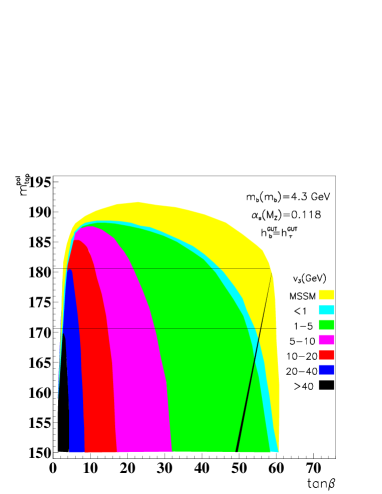
Figure 2: Top quark mass as a function of $\tan\beta$ for different values of the R–Parity violating parameter $v_{3}$.

5.3 On $\alpha_{s}(M_{Z})$ versus $\sin^{2}\theta_{W}(M_{Z})$

Recent studies of gauge coupling unification in the context of MSSM agree that using the experimental values for the electromagnetic coupling and the weak mixing angle, we get the prediction

$$\alpha_{s}(M_{Z})\sim 0.129\pm 0.010$$ (73)

that it is about 1$\sigma$ larger than indicated by the most recent world average value

$$\alpha_{s}(M_{Z})^{W.A}=0.1189\pm 0.0015$$ (74)

We have re-considered [20] the $\alpha_{s}$ prediction in the context of the model with bilinear breaking of R–Parity. We have shown that in this simplest R–Parity breaking model, with the same particle content as the MSSM, there appears an additional negative contribution to $\alpha_{s}$, which can bring the theoretical prediction closer to the experimental world average. This additional contribution comes from two–loop b–quark Yukawa effects on the renormalization group equations for $\alpha_{s}$. Moreover we have shown that this contribution is typically correlated to the tau–neutrino mass which is induced by R–Parity breaking and which controls the R-Parity violating effects. We found that it is possible to get a 5% effect on $\alpha_{s}(M_{Z})$ even for light $\nu_{\tau}$ masses. This is shown in Fig. 3 where we compare the predictions of $\alpha_{s}(M_{Z})$ in the MSSM and in the bilinear $\not{\!\!\!R}_{p}$ model.

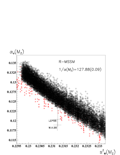
Figure 3: $\alpha_{s}(M_{Z})$ versus $\hat{s}_{Z}$ for the MSSM (circles) and for the bilinear $\not{\!\!\!R}_{p}$ model (crosses).

5.4 Neutrino Physics

In this model at tree-level only one neutrino picks up a mass via the mixing with the neutralinos. This result is exact but it can best be seen in the limit where the $R_{p}/\;\>$ parameters are small compared with the SUSY parameters [21],

$$\epsilon_{i},gv_{i},g^{\prime}v_{i}\ll M_{1},M_{2},\mu$$ (75)

Then we can write an effective neutrino $3\times 3$ matrix (see–saw)

$$m_{eff}\!=\!\frac{M_{1}g^{2}\!\!+\!\!M_{2}{g^{\prime}}^{2}}{4\,\det({\cal M}_{\chi^{0}})}\left(\!\!\begin{array}[]{ccc}\Lambda_{e}^{2}\!\!&\!\!\Lambda_{e}\Lambda_{\mu}\!\!&\!\!\Lambda_{e}\Lambda_{\tau}\\ \Lambda_{e}\Lambda_{\mu}\!\!&\!\!\Lambda_{\mu}^{2}\!\!&\!\!\Lambda_{\mu}\Lambda_{\tau}\\ \Lambda_{e}\Lambda_{\tau}\!\!&\!\!\Lambda_{\mu}\Lambda_{\tau}\!\!&\!\!\Lambda_{\tau}^{2}\end{array}\!\!\right)$$ (76)

where $\det({\cal M}_{\chi^{0}})$ is the determinant of the MSSM neutralino mass matrix and

$$\Lambda_{i}=\mu v_{i}+v_{d}\epsilon_{i}$$ (77)

The projective nature of $m_{eff}$ ensures that we get two zero eigenvalues. The only non–zero is

$$m_{\nu}=Tr(m_{eff})=\frac{M_{1}g^{2}+M_{2}{g^{\prime}}^{2}}{4\,det({\cal M}_{\chi^{0}})}|{\vec{\Lambda}}|^{2}.$$ (78)

At 1–loop level the two massless neutrinos get masses. The masses and mixings can be shown [16] to be compatible with those needed to solve the solar and atmospheric neutrino problems. We refer to the talk of M. Hirsch at this Conference [22] for the details.

5.5 Results at the Accelerators

We have extensivley studied the implications of the BRpV model at the accelerators [14, 6]. For instance an important prediction of the BRpV model is that the chargino can be single produced. The prediction for the NLC is shown in Fig. 4

Figure 4: Maximum single chargino production cross section as a function of the chargino mass at NLC in BRpV. Light and heavy charginos are displayed.

Here we will not describe these results any further but we emphasize that if R-parity is violated, the neutralino is unstable. As it shown in Fig. 5 it decays inside the detector. This is very important because its decays can serve as probes for the solar neutrino parameters [22, 23].

Figure 5:

6 Conclusions

We have shown that there is a viable model for SBRP that leads to a very rich phenomenology, both at laboratory experiments, and at present (LEP) and future (LHC, LNC) accelerators. In these models the radiative breaking of both the Gauge Symmetry and R-Parity can be achieved. Most of these phenomenology can be described by an effective model with explicit R–Parity violation. This model has many definite predictions that are different from the MSSM. In particular $b-\tau$ can be achieved for any value of $\tan\beta$ and we get a better prediction for $\alpha_{s}(M_{Z})$ then in the MSSM. We have calculated the one–loop corrected masses and mixings for the neutrinos and we get that these have the correct features to explain both the solar and atmospheric neutrino anomalies. We emphasize that the lightest neutralino decays inside the detectors, thus leading to a very different phenomenology than the MSSM. In particular the neutrino parameters can be tested at the accelerators.

References

- [1] Yu. A. Gol’fand and E. P. Likhtman, Sov. Phys. JETP Lett. 13 (1971) 323; D.V. Volkov and V.P. Akulov, Sov. Phys. JETP Lett. 16 (1972) 438; J. Wess and B. Zumino, Nucl. Phys. B 70 (1974) 39.
- [2] H.P. Nilles, Phys. Rep. 110 (1984) 1; H.E. Haber and G.L. Kane, Phys. Rep. 117 (1985) 75; R. Barbieri, Riv. Nuovo Cimento 11 (1988) 1.
- [3] C Aulakh, R Mohapatra, Phys. Lett. B 119 (1983) 136; A Santamaria, J W F Valle, Phys. Lett. B 195 (1987) 423; Phys. Rev. Lett. 60 (1988) 397; Phys. Rev. D 39 (1989) 1780.
- [4] A Masiero, J W F Valle, Phys. Lett. B 251 (1990) 273.
- [5] J.C. Romão, C.A. Santos, J.W.F. Valle, Phys. Lett. B 288 (1992) 311;
- [6] A Lopez-Fernandez, J. Romão, F. de Campos and J. W. F. Valle, Phys. Lett. B 312 (1993) 240; ibidem, Proceedings of Moriond ’94. pag.81-86, edited by J. Tran Thanh Van, Éditions Frontiéres, 1994. J. C. Romão, F. de Campos, M. A. Garcia-Jareno, M. B. Magro and J. W. F. Valle, Nucl. Phys. B 482 (1996) 3.
- [7] J C Romão, N Rius and J W F Valle, Nucl. Phys. B 363 (1991) 369.
- [8] For a review see e.g J. C. Romão, Lectures given at the 5th Gleb Wataghin School on High-Energy Phenomenology, Campinas, Brazil, 13-17 Jul 1998. e-Print Archive: hep-ph/9811454.
- [9] P Nogueira, J C Romão, J W F Valle, Phys. Lett. B 251 (1990) 142.
- [10] J. C. Romão, J. W. F. Valle, Nucl. Phys. B 381 (1992) 87.
- [11] S. Bertolini and G. Steigman, Nucl. Phys. B 387 (1990) 193; M. Kawasaki et al, Nucl. Phys. B 402 (1993) 323; Nucl. Phys. B 419 (1994) 105; S. Dodelson, G. Gyuk and M.S. Turner, Phys. Rev. D 49 (1994) 5068.
- [12] A. D. Dolgov, S. Pastor, J.C. Romão and J. W. F. Valle, Nucl. Phys. B 496 (1997) 24.
- [13] F. de Campos, M.A. García-Jareño, A.S. Joshipura, J. Rosiek, and J. W. F. Valle, Nucl. Phys. B 451 (1995) 3;T. Banks, Y. Grossman, E. Nardi, and Y. Nir, Phys. Rev. D 52 (1995) 5319; A. S. Joshipura and M.Nowakowski, Phys. Rev. D 51 (1995) 2421; R. Hempfling, Nucl. Phys. B 478 (1996) 3; F. Vissani and A.Yu. Smirnov, Nucl. Phys. B 460 (1996) 37; H. P. Nilles and N. Polonsky, Nucl. Phys. B 484 (1997) 33; B. de Carlos, P. L. White, Phys. Rev. D 55 (1997) 4222; S. Roy and B. Mukhopadhyaya, Phys. Rev. D 55 (1997) 7020.
- [14] A. Akeroyd, M.A. Díaz, J. Ferrandis, M.A. Garcia–Jareño, and Jose W.F. Valle, Nucl. Phys. B 529 (1998) 3.
- [15] M.A. Díaz, talk given at International Europhysics Conference on High Energy Physics, Jerusalem, Israel, 1997, hep-ph/9712213.
- [16] M.A. Díaz, M. Hirsch, W. Porod, J.C. Romão and J.W.F. Valle, Phys. Rev. D 61 (2000) 071703 [hep-ph/9907499]; M. Hirsch, M.A. Díaz, W. Porod, J.C. Romão and J.W.F. Valle, Phys. Rev. D 62 (2000) 113008 [hep-ph/0004015].
- [17] R. Hempfling, Nucl. Phys. B 478 (1996) 3.
- [18] M.A. Díaz, J.C. Romão, and J.W.F. Valle, Nucl. Phys. B 524 (1998) 23.
- [19] M.A. Díaz, J. Ferrandis, J.C. Romão, and J.W.F. Valle, Phys. Lett. B 453 (1999) 263.
- [20] M.A. Díaz, J. Ferrandis, J.C. Romão, and J.W.F. Valle, Nucl. Phys. B 590 (2000) 3.
- [21] M. Hirsch, J.W.F. Valle, Nucl. Phys. B 557 (1999) 60, [hep-ph/9812463].
- [22] See M. Hirsch talk at this Conference.
- [23] W. Porod, M. Hirsch, J.C. Romão and J.W.F. Valle, hep-ph/0011248.